Embed Size (px)
Citation preview

The University of ChicagoThe Booth School of Business of the University of ChicagoThe University of Chicago Law School
Identifying the Effect of Unemployment on CrimeAuthor(s): Steven Raphael and Rudolf Winter‐EbmerSource: Journal of Law and Economics, Vol. 44, No. 1 (April 2001), pp. 259-283Published by: The University of Chicago Press for The Booth School of Business of the University ofChicago and The University of Chicago Law SchoolStable URL: http://www.jstor.org/stable/10.1086/320275 .
Accessed: 27/03/2015 18:09
Your use of the JSTOR archive indicates your acceptance of the Terms & Conditions of Use, available at .http://www.jstor.org/page/info/about/policies/terms.jsp
.JSTOR is a not-for-profit service that helps scholars, researchers, and students discover, use, and build upon a wide range ofcontent in a trusted digital archive. We use information technology and tools to increase productivity and facilitate new formsof scholarship. For more information about JSTOR, please contact [email protected].
.
The University of Chicago Press, The University of Chicago, The Booth School of Business of the University ofChicago, The University of Chicago Law School are collaborating with JSTOR to digitize, preserve and extendaccess to Journal of Law and Economics.
http://www.jstor.org
This content downloaded from 199.190.174.232 on Fri, 27 Mar 2015 18:09:18 PMAll use subject to JSTOR Terms and Conditions

259
[Journal of Law and Economics, vol. XLIV (April 2001)]� 2001 by The University of Chicago. All rights reserved. 0022-2186/2001/4401-0010$01.50
IDENTIFYING THE EFFECT OFUNEMPLOYMENT ON CRIME*
STEVEN RAPHAELUniversity ofCalifornia,Berkeley
and RUDOLF WINTER-EBMERUniversity of Linz andCenter for Economic
Policy Research, London
Abstract
In this paper, we analyze the relationship between unemployment and crime. UsingU.S. state data, we estimate the effect of unemployment on the rates of seven felonyoffenses. We control extensively for state-level demographic and economic factors andestimate specifications that include state-specific time trends, state effects, and year effects.In addition, we use prime defense contracts and a state-specific measure of exposure tooil shocks as instruments for unemployment rates. We find significantly positive effectsof unemployment on property crime rates that are stable across model specifications. Ourestimates suggest that a substantial portion of the decline in property crime rates duringthe 1990s is attributable to the decline in the unemployment rate. The evidence for violentcrime is considerably weaker. However, a closer analysis of the violent crime of rapeyields some evidence that the employment prospects of males are weakly related to staterape rates.
I. Introduction
In 1998, the total crime index calculated by the Federal Bureau of Investigation(FBI) fell for the seventh straight year. Moreover, between 1993 and 1998, vic-timization rates declined for every major type of crime,1 with both violent andproperty crime rates falling by approximately 30 percent. Occurring concurrentlywith these aggregate crime trends was a marked decrease in the civilian un-employment rate. Between 1992 and 1998, the national unemployment rate de-clined in each year from a peak of 7.5 percent to a 30-year low of 4.5 percent.
The concurrence of these crime and labor market trends suggests that recent
* We would like to thank Cynthia Bansak, Reiner Buchegger, Horst Entorf, Thomas Marvell,Daniel Nagin, Lorien Rice, Eugene Smolensky, and Josef Zweimuller, as well as participants at the1999 New York American Economics Association meetings, the Center for Economic Policy Researchsummer workshop, the Verein fur Socialpolitik meeting,and seminars at Bonn, Linz, and Torino forseveral helpful suggestions. We thank Lawrence Katz, Mark Hooker, Carlisle Moody, and ChristopherRuhm for providing us with state level data. This research was supported by a grant from the AustrianFFF, grant P II962-SOZ.
1 Callie M. Rennison, Criminal Victimization 1998: Changes 1997–1998 with Trends 1993–1998(U.S. Dep’t Justice Rep. No. NCJ-1766353, 1999).
This content downloaded from 199.190.174.232 on Fri, 27 Mar 2015 18:09:18 PMAll use subject to JSTOR Terms and Conditions

260 the journal of law and economics
declines in crime rates may be due in part to the current abundance of legalemployment opportunities. To the extent that increased legitimate employmentopportunities deter potential offenders from committing crimes, a decline in theunemployment rate such as that observed during the 1990s may be said to causethe declines in crime rates. Despite the intuitive appeal of this argument, empiricalresearch to date has been unable to document a strong effect of unemploymenton crime. Studies of aggregate crime rates generally find small and statisticallyweak unemployment effects, with stronger effects for property crime than forviolent crime.2 In fact, several studies find significant negative effects of un-employment on violent crime rates, especially murder.3
There are several reasons to suspect that the available evidence understatesthe effect of unemployment on crime. Given that much of the previous researchrelies on time-series variation in macroeconomic conditions, the failure to controlfor variables that exert procyclical pressure on crime rates may downwardly biasestimates of the unemployment-crime effect. For example, alcohol consumptionvaries procyclically4 and tends to have independent effects on criminal behavior.5
Similar patterns may exist for drug use6 and gun availability. In addition, decliningincomes during recessions reduce purchases of consumer durables and otherpossible theftworthy goods, thus providing fewer targets for criminal activity. Ifone were only interested in the question “How much should we expect crime torise in the next recession?” then the reduced-form ordinary least squares (OLS)estimates would suffice. However, to assess the effect of unemployment on thepropensity to engage in criminal activities (the crime supply function), we muststatistically sort out these other effects.
2 Reviewing 68 studies, Theodor Chiricos, Rates of Crime and Unemployment: An Analysis ofAggregate Research Evidence, 34 Soc. Prob. 187 (1987), shows that fewer than half find positivesignificant effects of aggregate unemployment rates on crime rates. More recently, Horst Entorf &Hannes Spengler, Socioeconomic and Demographic Factors of Crime in Germany: Evidence fromPanel Data of the German States, 20 Int’l Rev. L. & Econ. 75 (2000), using a state panel for Germanyalso find ambiguous unemployment effects. Likewise, Kerry Papps & Rainer Winkelmann, Unem-ployment and Crime: New Answers to an Old Question (working paper, Univ. Canterbury 1998),finds little effect for a panel of regions from New Zealand. On the other hand, research looking atthe relationship between criminal participation and earnings potential finds stronger effects. JeffGrogger, Market Wages and Youth Crime, 16 J. Lab. Econ. 756 (1998), estimates a structural modelof time allocation between criminal, labor market, and other nonmarket activities and finds strongevidence that higher wages deter criminal activity. Further evidence supporting an effect of lowwages is provided in a panel study of U.S. counties, Eric D. Gould, Bruce A. Weinberg, & DavidB. Mustard, Crime Rates and Local Labor Market Opportunities in the United States: 1977–1997,Rev. Econ. & Stat. (forthcoming 2001). Michael Willis, Unemployment, the Minimum Wage andCrime. (working paper, Univ. California, Santa Barbara 1999), looks at the effect of minimum wageson property crime.
3 Philip J. Cook & Gary A. Zarkin, Crime and the Business Cycle, 14 J. Legal Stud. 115 (1985).4 Christopher J. Ruhm, Economic Conditions and Alcohol Problems, 14 J. Health Econ. 583 (1995).5 David A. Boyum & Mark A. R. Kleiman, Alcohol and Other Drugs, in Crime 295 (James Q.
Wilson & Joan Petersilia eds. 1995).6 Hope Corman & H. Naci Mocan, A Time-Series Analysis of Crime, Deterrence and Drug Abuse
in New York City, 90 Am. Econ. Rev. 584 (2000).
This content downloaded from 199.190.174.232 on Fri, 27 Mar 2015 18:09:18 PMAll use subject to JSTOR Terms and Conditions

unemployment effect 261
An additional problem associated with interpreting the empirical relationshipbetween unemployment and crime concerns the direction of causation. To theextent that criminal activity reduces the employability of offenders, through eithera scarring effect of incarceration or a greater reluctance among the criminallyinitiated to accept legitimate employment, criminal activity may in turn contributeto observed unemployment. Moreover, crime level may itself impede employmentgrowth and contribute to regional unemployment levels.7 Hence, in addition toproblems associated with omitted variables, previous inferences may also beflawed owing to simultaneity bias.8 To be more precise, simultaneity upwardlybiases OLS estimates of the causal effect of unemployment on crime.
In this paper we estimate the effect of unemployment rates on crime ratesusing a state-level panel covering the period 1971–97. We first use OLS re-gressions to estimate the effect of unemployment rates on the rates of the sevenfelony offenses recorded in the FBI’s Uniform Crime Reports (UCR). To mitigateomitted-variables bias, we take two precautions: (1) we control extensively forobservable demographic and economic variables, and (2) we exploit the panelaspects of our data by estimating models that allow for state and year fixed effectsas well as state-specific linear and quadratic time trends. In addition, we presenttwo-stage least squares (2SLS) estimates using state military contracts and ameasure of state exposure to oil shocks as instruments for unemployment rates.For property crime rates, the results consistently indicate that unemploymentincreases crime. The magnitude of these effects is stable across specificationsand ranges from a 1 to a 5 percent decline in crime caused by a 1 percentagepoint decrease in unemployment. For violent crime, however, the results aremixed, with some evidence of positive unemployment effects on robbery andassault and the puzzling findings of negative unemployment effects for murderand rape.
In an attempt to resolve this latter paradox, we exploit the specific features of
7 John Bound & Richard B. Freeman, What Went Wrong? The Erosion of Relative Earnings andEmployment among Young Black Men in the 1980s, 107 Q. J. Econ. 201 (1992); and Daniel Nagin& Joel Waldfogel, The Effects of Criminality and Conviction on the Labor Market Status of YoungBritish Offenders, 15 Int’l Rev. L. & Econ. 109 (1995), find that conviction and incarceration increasesthe probability of future unemployment. Jeffrey Grogger, The Effect of Arrest on the Employmentand Earnings of Young Men, 110 Q. J. Econ. 51 (1995), finds small and short-lived employmentimpacts of arrests. Michael Willis, Crime and the Location of Jobs (working paper, Univ. California,Santa Barbara 1999), finds that business formation and location is sensitive to local crime rates.Scott Freeman, Jeffrey Grogger, & Jon Sonstelie, The Spatial Concentration of Crime, 40 J. Urb.Econ. 216 (1996), presents a multiple-equilibrium model where an exogenous increase in crimereduces the probability of getting caught, thus altering the returns to criminal activity relative tolegitimate opportunities.
8 Simultaneity between crime and unemployment has been addressed in time-series studies byHope Corman, Theodor Joyce, & Norman Lovitch, Crime, Deterrence and the Business Cycle inNew York City: A VAR Approach, 69 Rev. Econ. & Stat. 695 (1987); and Shawn Bushway & JohnEngberg, Panel Data VAR Analysis of the Relationship between Crime and Unemployment (workingpaper, Carnegie Mellon Univ. 1995). Whereas the former finds no Granger causality in both directionsusing monthly data for New York City, the latter finds two-way Granger causality using annual timeseries for 103 counties in Pennsylvania and New York from 1976 to 1986.
This content downloaded from 199.190.174.232 on Fri, 27 Mar 2015 18:09:18 PMAll use subject to JSTOR Terms and Conditions

262 the journal of law and economics
rape offenses. A real behavioral effect of unemployment on the propensity tocommit violent acts may be statistically veiled by the effect of procyclical var-iation in the degree of interpersonal exposure of possible victims to potentialoffenders. This greater exposure may result from the fact that when more peopleare working and away from home, the quantity of encounters with potentialoffenders increases. Noting that in the overwhelming majority of rapes recordedin the UCR the perpetrator is male while the victim is always female, we firsttest for an empirical relationship between the rape rate and female unemploymentrates. To the extent that a negative relationship still exists, we can be certain thatthe negative correlation between female unemployment and rape does not reflectthe behavior of offenders but rather some other omitted factor that varies withregional employment cycles, such as an increase in the quantity of interpersonalinteractions. Next, we add female unemployment rates to model specificationsof the rape rate that include male unemployment rates. Here, the female un-employment rate serves as a control for all omitted factors not captured by theother control variables. The results from this exercise generally indicate that aftercontrolling for female unemployment rates, the effect of male unemploymentrates on rape are either positive or insignificant.
II. Unemployment, Crime, and Time Allocation
The proposition that unemployment induces criminal behavior is intuitivelyappealing and grounded in the notion that individuals respond to incentives.Conceptualizing criminal activity as a form of employment that requires timeand generates income,9 a “rational offender” should compare returns to time usein legal and illegal activities and make decisions accordingly. Holding all elseequal, the decrease in income and potential earnings associated with involuntaryunemployment increases the relative returns to illegal activity.
To more formally illustrate the relationship between unemployment and crime,Figures 1A and 1B present a model of time allocation following that of JeffGrogger.10 In Figure 1A, the individual has discretion over A hours of time andnonlabor income equal to the distance AB. The person converts nonmarket timeinto income by engaging in either legitimate employment or income-generatingcriminal activity. The returns to crime are diminishing and are given by thecurved segment BCE. Diminishing returns follows from the assumption of ra-tional choice: individuals first commit crimes with the highest expected payoffs(lowest probability of getting caught and highest stakes) before exploring lesslucrative opportunities. Assuming that the returns to allocating a small amountof time to criminal activity exceed potential wages, the individual would supplytime to the legitimate labor market only after higher-paying criminal opportunities
9 Ann Dryden Witte & Helen Tauchen, Work and Crime: An Exploration Using Panel Data(Working Paper No. 4794, NBER 1994).
10 Grogger, supra note 2.
This content downloaded from 199.190.174.232 on Fri, 27 Mar 2015 18:09:18 PMAll use subject to JSTOR Terms and Conditions

unemployment effect 263
Figure 1
have been fully exploited. This occurs at the point C where the person hasallocated time to crime and where the marginal return to crime equalsA � t0
potential wages. Beyond point C, wages exceed the returns to criminal activity(as is evident by the steeper slope of the budget constraint segment CD).
The budget constraint differs from that of a standard model of the labor-leisurechoice in its implicit recursive structure. The individual first locates the pointthat equates the marginal returns to legitimate and illegitimate activities. Timeallocations to the right of this point involve criminal activity only, while timeallocations that exceed this level (to the left of ) involve a mix of work in thet0
legitimate market and time supplied to criminal activity. When there are nobarriers to employment, the budget constraint is given by ABCD. In Figure 1A,the individual maximizes utility by devoting time to criminal activity andA � t0
supplying time to the labor market. For those for whom the returns tot � t0 1
crime never exceed potential wages in the legitimate labor market, the budgetconstraint is simply that of the standard labor-leisure model. This is depicted inFigure 1B, where the marginal income generated by criminal activity (given bythe curve BD) is always less than the income generated by an additional hourof legitimate work (line BC).
This model can be used to illustrate how unemployment affects crime ratesby analyzing the possible behavioral responses to an unemployment spell. Forindividuals with relatively low potential wages (initial returns to crime exceedwages), unemployment shifts the budget constraint from ABCD to ABCE.Whether this increases time allocated to criminal activity depends on the indi-vidual’s preferences. For the person depicted in Figure 1A, such a shift unam-biguously increases the time devoted to criminal activity. Since the optimal timeallocation decision in the absence of unemployment occurs to the left of pointC, the indifference curve representing the utility level at point C ( ) crossesU1
the budget constraint with a relatively flatter slope—that is to say, the marginal
This content downloaded from 199.190.174.232 on Fri, 27 Mar 2015 18:09:18 PMAll use subject to JSTOR Terms and Conditions

264 the journal of law and economics
rate of substitution between nonmarket time and income at point C is less thanthe marginal rate at which the individual can convert time into income via bothlegitimate and illegitimate activity. For both constraints ABCD and ABCE, thisindividual will sacrifice more nonmarket time than the amount given by A �
. Hence, for persons that engage in criminal activity while working, the modelt0
predicts that unemployment increases time allocated to crime.11 On the otherhand, for an individual facing the constraints in Figure 1A who engages in onlycriminal activity (or engages in neither legitimate nor illegitimate activities),unemployment does not affect the time allocated to crime.
For those workers with wages that always exceed the marginal return to crime,unemployment shifts the budget constraints in Figure 1B from ABC to ABD.Here, whether or not the individual commits crime as a result of the unemploy-ment spell depends on whether the return to the initial hour of criminal activityexceeds his or her reservation wage. Individuals with relatively high reservationwages will be unlikely to commit crimes as a result of an unemployment spell.On the other hand, individuals with relatively low reservation wages are morelikely to attempt to offset income lost owing to unemployment through criminalactivity.
In sum, the theoretical model yields four possible types of individuals roughlydefined by potential earnings in the labor market relative to the returns to criminalactivity and preferences over income and nonmarket time. The theory predictsthat for two of these four categories, an unemployment spell will increase timeallocated to criminal activity (and thus increase the crime rate), while for theremaining two categories, there is no response to an unemployment spell. In theaggregate, while the relationship between unemployment and crime rates shouldbe unambiguously positive, the magnitude of this relationship depends on thedistribution of the unemployed across these four categories. This is an empiricalquestion to which we now turn.
III. Empirical Strategy and Data Description
Our empirical strategy is to use a state-level panel data set to test for a re-lationship between state unemployment rates and the rates of the seven felonyoffenses. Our panel covers the period 1971–97 for the 50 states (Washington,D.C., is excluded).12 Since the main empirical tests rely on the aggregate reduced-form relationship between state unemployment rates and state crime rates, iso-lating the effect due to a behavioral response of the unemployed (that is to say,additional crimes committed by those suffering unemployment spells) requires
11 Grogger’s work, id., suggests that a substantial minority of employed out-of-school youthsengage in some income-generating criminal activity. In an analysis of National Longitudinal Surveyof Youth data, the author finds that nearly a quarter of the employed youths self-report committingcrimes.
12 For several states in the early 1970s, we are missing data on several explanatory variables.Hence, rather than having 1,350 observations for the 27-year period, we have 1,293 observations.
This content downloaded from 199.190.174.232 on Fri, 27 Mar 2015 18:09:18 PMAll use subject to JSTOR Terms and Conditions

unemployment effect 265
careful consideration of other factors that vary systematically with regional busi-ness cycles and that affect crime rates.
Philip Cook and Gary Zarkin13 suggest four categories of factors that mayempirically link the business cycle and crime: (1) legitimate employment op-portunities, (2) criminal opportunities, (3) consumption of criminogenic com-modities (alcohol, drugs, guns), and (4) the response of the criminal justicesystem. The crime effects of access to legitimate opportunities were the subjectof the previous section and are tautologically procyclical. The factors listed inthe latter three categories are also likely to vary with the business cycle. Thequality and quantity of criminal opportunities may be lower during recessionsas potential victims have less income, consume less, and expend more effort onprotecting what they have. If alcohol, drugs, and guns are normal goods, con-sumption of these goods will be procyclical. Furthermore, if these commoditiesinduce criminal behavior, or in the least augment the lethality of criminal inci-dents, procyclical consumption will induce procyclical variations in somecrimes.14 The extent of variation in policing and criminal justice activity overthe business cycle is less clear since the quantity and efficacy of criminal justiceactivity depends on state tax revenues, community cooperation, and politicalpressures.15
Omission of any of these factors from aggregate crime regressions may biasthe estimates of the relationship we seek to measure. For example, assuming thatthe consumption of drugs and alcohol is negatively correlated with unemploymentand positively correlated with crime, omitting these factors from the regressionwould bias estimates of the unemployment-crime effect downward. Similarly,procyclical variation in criminal opportunities would also create a downwardbias. To mitigate such omitted-variables bias, we control extensively for ob-servable state-level covariates and exploit the panel aspects of our data set tonet out variation in crime rates due to unobserved factors. The most completemodel specification that we estimate is given by the equation
2Crime p a � d � w time � q time � gUnemployed � bX � h , (1)it t i i t i t it it it
where i and t index states and years, Crimeit is the log of the number of crimesper 100,000 state residents, Unemployedit is the unemployment rate, is aXit
13 Cook & Zarkin, supra note 3.14 The effect of guns, drugs, and alcohol on violent and property crime is a matter of some debate.
Philip J. Cook & Mark H. Moore, Gun Control, in Wilson & Petersilia eds., supra note 5, at 267,notes that while guns do appear to increase lethality of criminal acts, the evidence concerning theeffect of gun availability on the overall level of crime is mixed. Concerning drugs and alcohol,Boyum & Kleiman, supra note 5, notes that in behavioral experiments alcohol is more consistentlyfound to lower inhibitions and increase aggressive behavior. Jeffrey Fagan, Intoxication and Ag-gression, in Drugs and Crime 241 (Michael H. Tonry & James Q. Wilson eds. 1990), notes that theevidence concerning the pharmacological effects of illegal drugs is mixed, with drugs such asmarijuana being more likely to reduce aggressive behavior.
15 Steven D. Levitt, Using Electoral Cycles in Police Hiring to Estimate the Effect of Police onCrime, 87 Am. Econ. Rev. 270 (1997).
This content downloaded from 199.190.174.232 on Fri, 27 Mar 2015 18:09:18 PMAll use subject to JSTOR Terms and Conditions

266 the journal of law and economics
vector of standard controls, is a year fixed effect, is a state fixed effect,a dt i
timet and are linear and quadratic time trends, gives the state-specific2time wi i
coefficient on the linear trend while gives the state-specific coefficient on theqi
quadratic time trend, g is the semielasticity of the crime rate with respect to theunemployment rate, b is the vector of parameters for the control variables in
, and is the residual.X hit it
We explicitly control for several variables. First, to account for procyclicalconsumption of criminogenic commodities, we include a measure of alcoholconsumption per capita (measured in gallons of ethanol) and the average incomeper worker (personal income divided by employment) for each state-year. Whilewe would like to directly control for drug consumption and gun availability,these data are unavailable. Hence, we use income per worker to proxy for var-iation in consumption of criminogenic commodities.16 We also include controlsfor the proportion of state residents that are black, living in poverty, and residingin metropolitan areas. To adjust for the effect of age structure on aggregate crimerates, we include seven variables that measure the distribution of the state pop-ulation across age categories. Given the well-documented age-crime profile,17
these controls are needed to ensure that estimates of the crime-unemploymenteffect are not contaminated by changes in state age structures.
Finally, we include the incarceration rate in state prisons in all models. Apositive effect of unemployment on crime is likely to lead to a positive correlationbetween unemployment and prison populations (assuming that some offendersare caught and sent to prison). If incarceration reduces crime rates via incapac-itation and deterrence (a proposition supported by Steven Levitt),18 omittingincarceration rates from equation (1) would downwardly bias the unemployment-crime effect. In all models, we enter prison populations per 100,000 state residentsmeasured in log units.
To be sure, our list of control variables is likely to be incomplete, as it isimpossible to observe all factors that affect crime and vary with regional cycles.To adjust further for unobservable variables, we exploit the panel aspects of ourdata set. By including state effects, we eliminate all variation in crime ratescaused by factors that vary across states yet are constant over time, while theinclusion of year effects eliminates the influence of factors that cause year-to-year changes in crime rates common to all states. State-specific linear and quad-ratic time trends (following Leora Friedberg)19 eliminate variation in within-state
16 We also estimated all of our models using income per capita rather than income per worker.This did not change the results.
17 David F. Greenberg, Age, Crime, and Social Explanation, 91 Am. J. Soc. 1 (1985); Grogger,supra note 2; Travis Hirshi & Michael Gottfredson, Age and the Explanation of Crime, 89 Am. J.Soc. 552 (1983).
18 Steven D. Levitt, The Effect of Prison Population Size on Crime Rates: Evidence from PrisonOvercrowding Litigation, 111 Q. J. Econ. 319 (1996).
19 Leora Friedberg, Did Unilateral Divorce Raise Divorce Rates? Evidence from Panel Data, 88Am. Econ. Rev. 608 (1998), employs a similar panel specification.
This content downloaded from 199.190.174.232 on Fri, 27 Mar 2015 18:09:18 PMAll use subject to JSTOR Terms and Conditions

unemployment effect 267
crime rates caused by factors that are state specific over time. In these models,the unemployment-crime effects are identified using within-state variation in theunemployment rate (relative to the national rate) after netting out state-specifictime trends. This is a particularly flexible specification that should certainlyeliminate the influence of many unobserved factors.
An alternative approach that addresses omitted-variables bias would be to findinstrumental variables that determine state unemployment rates yet are unrelatedto possible contaminating omitted factors and to reestimate equation (1) using2SLS. This approach carries the added benefit that the direction of causality isclearly established. As discussed above, the direction of causation may run fromcrime to unemployment. This would be the case if (former) criminals becomeunemployable or if high crime rates discourage employment growth and driveaway existing firms, thus contributing to a state’s unemployment rate.
Hence, to rule out reverse causation we estimate the crime-unemploymentrelationship using the specification discussed above but instrumenting state un-employment rates. We employ two instruments: Department of Defense (DOD)annual prime contract awards to each state and a state-specific measure of oilprice shocks. The annual prime contract awards are measured in thousands ofdollars per capita. Our measure of state-specific oil price shocks is constructedas follows. For each state and each year, we start with a variable measuring theproportion of employment in the manufacturing sector, MANit. This provides arough measure of the importance of energy intensive industries where fuel costsare likely to be a relatively substantial component of production costs. Next,following Mark Hooker and Michael Knetter20 we construct an annual variableindicating changes in the relative price of crude oil, OILt, by dividing the producerprice index for crude oil by the gross domestic product deflator. Multiplyingthese two variables provides our measure of state-specific exposure to oil shocks( ). The effects of both the prime contracts and oilOil Costs p MAN # OILit it t
costs variables on state unemployment rates have been well documented by pastresearch.21
To be valid, the instruments must be exogenous determinants of unemploymentrates and cannot be correlated with any omitted variables contained in the residualof the second-stage crime equation. Both variables appear to be exogenous de-terminants of unemployment. Oil prices are determined on world markets andhence should not be influenced by the unemployment rate in any one state andyear. Moreover, it is unlikely that state unemployment rates affect the industrial
20 Mark A. Hooker & Michael M. Knetter, The Effects of Military Spending on Economic Activity:Evidence from State Procurement Spending, 28 J. Money Credit & Banking 400 (1997).
21 Olivier Jean Blanchard & Lawrence F. Katz, Regional Evolution, Brookings Papers Econ.Activity no. 1, at 1 (1992); Mark A. Hooker & Michael M. Knetter, Unemployment Effects ofMilitary Spending: Evidence from a Panel of States (Working Paper No. 4889, NBER 1994); Hooker& Knetter, supra note 20; Steven J. Davis, Prakash Loungani, & Ramamohan Malidhara, RegionalLabor Fluctuations: Oil Shocks, Military Spending, and other Driving Forces (IF Working PaperNo. 578, Board of Governors Fed. Reserve Sys. 1997).
This content downloaded from 199.190.174.232 on Fri, 27 Mar 2015 18:09:18 PMAll use subject to JSTOR Terms and Conditions

268 the journal of law and economics
structure of a state’s employment base, though causation may clearly run in theopposite direction.
The question of whether defense spending exogenously determines unem-ployment rates boils down to the issue of whether the defense appropriationsprocess is influenced by fiscal policy concerns. At the national level, this doesnot appear to be the case.22 However, even if national defense spending is affectedby national unemployment rates, including year fixed effects in the crime modelspecification will eliminate any contamination of the instrument from this source.A more important issue concerns whether the spatial distribution of contractawards, holding aggregate appropriation constant, is determined in part by de-viations in state unemployment rates from the national rate. Steven Davis, PrakashLoungani, and Ramamohan Malidhara23 cite several detailed case studies thatindicate that this is unlikely. Hence, here we will follow the lead of recentmacroeconomic and regional economic research and assume that state-level con-tract awards are exogenous with respect to state unemployment rates.
Whether our instrumental variables are correlated with unobserved determi-nants of crime rates that are swept into the second-stage residuals is a moredifficult question. For unobserved determinants that are spuriously correlatedwith unemployment rates, this is unlikely to be a problem. However, if certainomitted factors are themselves determined by unemployment rates (for example,drug consumption or gun availability), our instruments will be correlated withthe second-stage residuals. One would expect that unemployment affects theconsumption of criminogenic substances, as well as the consumption of durablegoods that provide criminal opportunities. If our control variables eliminate var-iation caused by these factors (alcohol consumption, income per worker, andvarious fixed effects and state trends), our 2SLS results should be valid. None-theless, we acknowledge this potential shortcoming.
The data for this project come from several sources. State data on seven felonyoffenses (murder, forcible rape, robbery, aggravated assault, burglary, larceny-theft, and motor vehicle theft) come from the FBI’s UCR. The annual incidenceof these seven offenses (expressed per 100,000 state residents) are the primarydependent variables of interest along with the total property crime (the sum of
22 Davis, Loungani, & Malidhara, supra note 21, shows that major shifts in defense spendingstrongly coincide with international developments affecting national security (the onset of the ColdWar, the military buildup under Carter and Reagan, and the defense cutbacks driven by the end ofthe Cold War) rather than the national unemployment. In addition, Kenneth R. Mayer, The PoliticalEconomy of Defense Contracting 183 (1991), presents a convincing argument that the defenseappropriations process renders altering defense spending for fiscal policy purposes quite difficult,noting (1) the appropriation process is long, often extending 2 years or more between initial DODrequests and congressional approval; (2) major portions of the defense budget are uncontrollablesince they are determined by the size of the armed forces, pay scales, and other factors that areimmutable for political purposes; and (3) the delay between congressional approval and the obligationof funds (the action that creates employment, according to David F. Greenberg, Employment Impactsof Defense Expenditures and Obligations, 49 Rev. Econ. & Stat. 186 (1967)) is lengthy and mayoccur several years after budget adoption.
23 Davis, Loungani, & Malidhara, supra note 21.
This content downloaded from 199.190.174.232 on Fri, 27 Mar 2015 18:09:18 PMAll use subject to JSTOR Terms and Conditions

unemployment effect 269
burglary, larceny-theft, and motor vehicle theft) and the total violent crime rates(the sum of murder, forcible rape, robbery, and aggravated assault). Annual datafor state population and age structure are from the Bureau of the Census. Statepoverty rates, the proportion of black residents, and the proportion of the statepopulation living in metropolitan areas are from the decennial censuses for censusyears and are interpolated for years between 1970, 1980, and 1990 and projectedforward for 1991–97. These data, compiled by Thomas B. Marvell, have beenused in the past to study the crime effects of enhanced prison terms and statedeterminate-sentencing policies.24
State unemployment rates from 1976 to 1997 for all states and from 1971 to1997 for the 10 largest states come from the Current Population Survey Geo-graphic Profile of Employment and Unemployment. The remaining unemploy-ment figures are constructed from Bureau of Labor Statistics unemployment ratesfor Labor Market Areas. Data for state personal income come from the Bureauof Economic Analysis, while data on total employment and manufacturing em-ployment come from the Bureau of Labor Statisitcs. Data on per capita alcoholconsumption come from the Alcohol Epidemiological Data System maintainedby the National Institute of Alcohol Abuse and Alcoholism, while data on stateprison populations come from the Bureau of Justice Statistics. Finally, data onprime defense contracts awarded to individual states come from Hooker andKnetter.25
Table 1 presents summary statistics for all variables.26 Property crime is farmore common than violent crime, with the highest crime rate being that forlarceny (2,883 incidents per 100,000 persons) and the lowest crime rate beingthat for murder (nine incidents per 100,000 persons). As can be seen by comparingthe figures in the second and fourth columns, much of the variation in crimerates is eliminated by controlling for fixed effects and time trends, although somevariation remains. Allowing for these effects and trends eliminates only half ofthe variation in state unemployment rates. For the more stable, slower changingvariables (age structure, poor, and black), netting out state and year effects elim-inates a considerably larger portion of the variance.
IV. Empirical Results
In this section we present our main results. First, we present OLS estimatesof the crime-unemployment effects for the total property and total violent crimerates followed by results for each of the seven individual felony offenses. Next,
24 Thomas B. Marvell & Carlisle E. Moody, The Impact of Enhanced Prison Terms for FeloniesCommitted with Guns, 33 Criminology 247 (1995); Thomas B. Marvell & Carlisle E. Moody,Determinate Sentencing and Abolishing Parole: The Long-Term Impacts on Prisons and Crime, 34Criminology 107 (1996).
25 Hooker & Knetter, supra note 20. Since all 2SLS models estimated below include year dummyvariables, we do not convert military expenditures to constant dollars. Doing so does not affect theresults.
26 All values in Table 1 are weighted by state populations as are all results presented below.
This content downloaded from 199.190.174.232 on Fri, 27 Mar 2015 18:09:18 PMAll use subject to JSTOR Terms and Conditions

270 the journal of law and economics
TABLE 1
Summary Statistics for Crime Rates and Explanatory Variables
Variables Mean Standard Deviation
Standard DeviationNet of State
and Time Effects
Standard DeviationNet of State andTime Effects andState Time Trendsa
Property crime 4,674.81 1,158.20 434.24 249.91Burglary 1,276.26 419.12 162.58 99.13Larceny 2,883.48 725.10 268.67 155.01Auto theft 515.07 229.48 92.77 56.02
Violent crime 585.51 264.35 68.85 42.05Murder 8.58 3.49 1.29 1.02Rape 34.36 11.67 5.97 3.76Robbery 220.07 132.17 29.81 21.31Assault 322.51 156.99 51.96 31.12
Unemployed .07 .02 .01 .01Prison population 214.03 134.13 45.36 18.08Alcohol consumption 1.98 .40 .15 .08Metropolitan .77 .17 .02 .01Poor .13 .04 .02 .01Black .11 .07 .01 .001Income per worker 33.39 14.13 2.32 .55Population age:
Under 15 .23 .03 .007 .00315–17 .05 .01 .002 .00118–24 .12 .02 .005 .00325–34 .16 .02 .007 .00335–44 .13 .02 .004 .00245–54 .11 ..01 .003 .00155–64 .09 .01 .003 .001
Military spending .38 .31 .14 .09Oil costs .16 .09 .03 .02
Note.—All crime rates and the incarceration rate in state prisons are defined per 100,000 state residents. Alcoholconsumption is measured in consumption of gallons of ethanol per capita. Income per worker and military spendingare measured in thousands of dollars per capita. The panel covers the period 1971–97. There are 1,293 observations.
a Standard deviations are net of linear and quadratic time trends.
we present comparable results instrumenting for state unemployment rates. Forall crimes, we estimate three models: models including state and year effects;models including state effects, year effects, and state-specific linear trends; andmodels including state effects, year effects, and linear and quadratic trends. Inaddition, all specifications include the variables (with the exception of the twoinstruments) listed in Table 1.
A. Ordinary Least Squares Regression Results
Table 2 presents regressions where the dependent variable is either the log ofthe total property crime rate or the log of the total violent crime rate. The firstthree columns provide the results for property crime, while the next three columnsprovide the results for violent crime. In all property crime models, the effect ofunemployment is positive and significant at the 1 percent level of confidence.
This content downloaded from 199.190.174.232 on Fri, 27 Mar 2015 18:09:18 PMAll use subject to JSTOR Terms and Conditions

unemployment effect 271
TABLE 2
Ordinary Least Squares Regressions of Total Property and Total Violent Crime onState Unemployment Rates and Variables Measuring State Demographic Structure
ln(Property Crime Rate) ln(Violent Crime Rate)
(1) (2) (3) (4) (5) (6)
Unemployed 2.345 1.680 1.635 .266 .392 .547(.205) (.192) (.182) (.295) (.297) (.275)
ln(prisoners) �.129 �.093 �.108 �.018 �.028 �.042(.015) (.014) (.015) (.021) (.022) (.022)
Alcohol consumption .207 �.147 �.129 .074 .048 .027(.023) (.028) (.028) (.034) (.044) (.043)
Metropolitan .875 .670 .145 .754 1.510 .922(.148) (.185) (.232) (.212) (.286) (.350)
Poor �1.081 �.207 .076 �.209 �.195 �.247(.156) (.131) (.128) (.223) (.202) (.194)
Black 1.508 �2.883 3.881 �3.475 �2.987 5.024(.414) (.807) (1.475) (.594) (1.246) (2.229)
Income per worker �.010 �.025 �.001 �.012 �.022 �.016(.001) (.002) (.004) (.002) (.004) (.005)
Population age:Under 15 �1.841 .817 .014 .016 �1.412 �4.006
(.469) (.479) (.637) (.674) (.739) (.963)15–17 8.338 14.379 10.360 7.064 4.729 9.758
(1.734) (1.700) (1.770) (2.487) (2.625) (2.676)18–24 .637 1.367 1.466 2.326 1.789 4.551
(.676) (.578) (.633) (.971) (.893) (.956)25–34 1.395 7.123 7.611 7.277 7.127 7.474
(.588) (.564) (.718) (.844) (.871) (1.086)35–44 �5.862 �1.666 �.525 1.174 .569 �6.398
(.756) (.890) (1.178) (1.086) (1.374) (1.781)45–54 2.206 5.508 4.825 �2.797 �2.805 �1.305
(.917) (1.096) (1.498) (1.315) (1.693) (2.264)55–64 �4.751 �5.189 �3.575 �.238 .376 7.120
(.974) (.921) (1.495) (1.397) (1.421) (2.261)Linear trends No Yes Yes No Yes YesQuadratic trends No No Yes No No Yes
Note.—Standard errors are in parentheses. The dependent variable in each regression is the log of the respectivecrime rate per 100,000 state residents. All regressions include a full set of state and year fixed effects. There are1,293 observations covering the period 1971–97.
The magnitude of the relationship indicates that a 1 percentage point drop in theunemployment rate causes a decline in the property crime rate of between 1.6and 2.4 percent.
The results for violent crime are mixed. In the first specification, the coefficientis small and insignificant. Adding linear time trends increases the point estimateof the unemployment coefficient, yet the variable is still insignificant at the 10percent level ( ). Finally, adding the quadratic time trends to thep-value p 0.18model increases the point estimate further, and the coefficient becomes significantat the 5 percent level of confidence. The fact that controlling for state-specifictrends increases the coefficient on unemployment suggests that the state-specific
This content downloaded from 199.190.174.232 on Fri, 27 Mar 2015 18:09:18 PMAll use subject to JSTOR Terms and Conditions
272 the journal of law and economics
crime trends driven by the omitted crime fundamentals tend to move in theopposite direction of the trends in unemployment rates over the time periodcovered by the panel.27 For the one specification where unemployment exhibitsa positive significant effect, the magnitude is considerably smaller than the com-parable estimate for property crime. The results in column (6) indicate that a 1percentage point decline in the unemployment rate causes a decline in the violentcrime rate of one-half of a percent.
Concerning the performance of the other variables listed in Table 2, prisonincarceration rates generally exert negative effects on crime rates. These effectsare significant for all of the property crime models but for only the final violentcrime model.28 Alcohol consumption is positive and significant in only one ofthe property crime models and one violent crime models. This effect is knockedout by including the state time trend variables. In all models, crime rates tendto be higher in states with larger metropolitan populations, while there are noconsistent patterns for the relationship between crime rates and either the pro-portion of poor residents or the proportion of black residents. Consistent withprevious research on the age-crime profile, both property and violent crime ratesare higher in states with higher proportions of teenagers and young adults.
Income per worker exhibits negative effects on both property and violent crimerates and is significant in all models with the exception of the property crimemodel presented in column (3). Recall that we included this variable in an attemptto proxy for income effects on the demand for criminogenic substances and,hence, expected to see positive coefficients. These consistent negative effectssuggest that the variable may be picking up the effect of an alternative dimensionof legitimate labor market opportunities, namely, earnings.
Table 3 presents separate estimates of the crime-unemployment effects for theseven specific crimes using the same three specifications. For reference, the resultsfor the total property and violent crime models are reproduced. Since the resultsfor the other control variables do not differ substantially from the patterns pre-sented in Table 2, we suppress this output in this and all remaining tables. Startingwith the three individual property crimes, the unemployment rate exerts positive
27 A simple statistical model illustrates this point. Suppose that for a two-state panel the true modelis given by , but we estimate the misspecifiedCrime p a � bUnemployed � w time � w time � �it it 1 t 2 t it
model, , omitting the time trends. The probability limit of theCrime p a � bUnemployed � git it it
OLS estimate is given by bOLS p ,b �cov(Unemployed , time )/var(Unemployed ) # (w � w )it t it 1 2
where the bias due to omitting the trends is given by the second term in the equation. If unemploymentis trending upward ( ) and the predominant state trend in crime rates iscov(Unemployed , time ) 1 0it t
negative ( ), then the OLS coefficient estimate will be biased downward (similarly ifw � w ! 01 2
unemployment trends downward and crime upward). Another instance where allowing for linear andquadratic trends in state panel data yields a significant effect for an otherwise insignificant variableis found in Friedberg, supra note 19. Investigating the effect of unilateral divorce laws on statedivorce rates, the author finds that adding state trends yields significant effects that were not presentin model specifications that included state and year effects only.
28 These effects are smaller than those found by Levitt, supra note 18. However, unlike the studyby Levitt, we have made no attempt to address the simultaneity bias to OLS estimates of the crime-prison elasticity.
This content downloaded from 199.190.174.232 on Fri, 27 Mar 2015 18:09:18 PMAll use subject to JSTOR Terms and Conditions

unemployment effect 273
TABLE 3
Ordinary Least Squares Estimates of the Semielasticities of SpecificCrimes with Respect to State Unemployment Rates
No StateTime Trends
(1)Linear Trends
(2)
Linear andQuadratic Trends
(3)
All property crime 2.345 1.680 1.635(.205) (.192) (.182)
Burglary 3.227 2.276 2.069(.251) (.251) (.243)
Larceny 2.335 1.467 1.494(.223) (.193) (.188)
Auto theft �.033 1.383 1.028(.468) (.462) (.406)
All violent crime .266 .392 .547(.295) (.297) (.275)
Murder �2.523 �.819 �.751(.439) (.477) (.467)
Rape 1.239 .092 �.744(.353) (.322) (.298)
Robbery .006 1.419 1.724(.443) (.433) (.415)
Assault .293 .083 .183(.379) (.385) (.362)
Note.—Standard errors are in parentheses. The parameter estimates are the coefficients on the state un-employment variable from regressions where the dependent variable is the log of the respective crime rate.Crime rates are measured per 100,000 state residents. All of the regressions include the control variable listedin Table 1 as well as full sets of state and year fixed effects. Each regression has 1,293 observations andcovers the period 1971–97.
and statistically significant effects (at the 1 percent level of confidence) in allmodels with the exception of the auto theft regression omitting the state-specifictrends. The magnitudes of the effects are very stable across specifications, againwith the exception of auto theft. For the auto theft rate, adding the trend variablesdrastically increases the magnitude and significance of the unemploymentrate, which points to a specific trend pattern in auto theft rates over time ascompared to other crime rates. For the most complete specification, the crime-unemployment semielasticities are quite similar across offenses. A 1 percentagepoint decrease in the unemployment rate causes a 2 percent decrease in burglary,a 1.5 percent decrease in larceny, and a 1 percent decrease in auto theft.
The results for the specific violent crimes are considerably more variable. Thecoefficient on unemployment is negative for all three murder models and sig-nificant in the first two, although adding the linear and quadratic time trendsdrastically reduces the magnitude of this effect. The results for rape are unstableacross specifications, with a positive significant effect in the first specification,an insignificant effect when linear trends are added, and a puzzling negative andsignificant effect when both linear and quadratic time trends are included in themodel. The results for robbery are stronger, with no significant effect when timetrends are omitted and significant (at 1 percent) positive effects in the two models
This content downloaded from 199.190.174.232 on Fri, 27 Mar 2015 18:09:18 PMAll use subject to JSTOR Terms and Conditions

274 the journal of law and economics
TABLE 4
First-Stage Regressions of State Unemployment Rateson State Military Contracts per Capita and
State-Level Measure of Oil Costs
(1) (2) (3)
Military spending �..012 �.007 �.004(.002) (.002) (.003)
Oil costs .091 .064 .088(.014) (.013) (.015)
Linear trends No Yes YesQuadratic trends No No YesF-statistica 31.783 16.571 19.377p-value .0001 .0001 .0001
Note.—Standard errors are in parentheses. All of the regressions include the controlvariables listed in Table 1 as well as full sets of state and year fixed effects. Eachregression has 1,293 observations and covers the period 1971–97.
a This is the test statistic (and p-value) from an F-test of the joint significance ofthe military spending and oil costs instrumental variables.
that include trends. The magnitude of the robbery-unemployment effects in thelast two models are similar to the property crime effects, a reassuring findingconsidering that robbery, while a violent crime in nature, is motivated by thedesire to steal someone else’s property. Finally, unemployment is insignificantin all three assault rate models.
To summarize, we find positive and highly significant effects of unemploymenton property crimes, both in the aggregate and for individual offenses. The mag-nitudes of these effects are generally consistent across specification.29 The resultsfor violent crime are considerably weaker. For the two most serious violent crimesof murder and rape, the effect of unemployment is either significant and wronglysigned or is unstable across specifications, while there are no measurable effectson the rate of assault and some evidence of a positive unemployment effect forburglary.
B. Two-Stage Least Squares Results
In this section, we present 2SLS estimates of the crime-unemployment semi-elasticities using military contracts and a state-specific measure of oil costs asinstruments for the state unemployment rate. Recall that if our model specifi-cations omit crime-determining factors that are correlated with unemploymentand that are not picked up by the fixed effects and trends variables, the OLSresults that we have presented thus far will be biased. Moreover, if crime ratesreverse cause unemployment rates, inferences from OLS results will be flawed.
Before discussing estimates of the unemployment effects, an evaluation of thestrength of the first-stage relationship is needed. Table 4 presents the results from
29 The relative importance of these effects in explaining recent changes in crime rates is a questionto which we will return in the conclusion.
This content downloaded from 199.190.174.232 on Fri, 27 Mar 2015 18:09:18 PMAll use subject to JSTOR Terms and Conditions
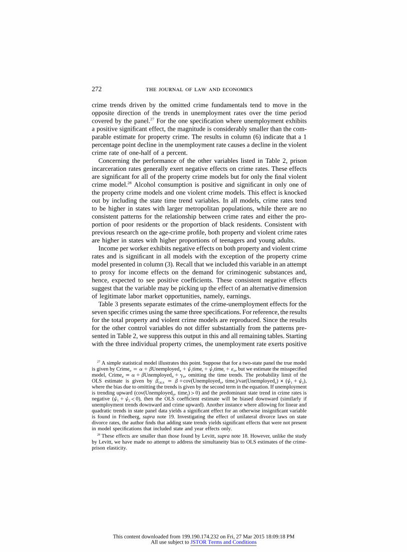
unemployment effect 275
TABLE 5
Ordinary and Two-Stage Least Squares Estimates of the Semielasticities ofSpecific Crimes with Respect to State Unemployment Rates
No State TimeTrends Linear Trends
Linear andQuadratic Trends
OLS 2SLS OLS 2SLS OLS 2SLS
All property crime 2.345 3.853 1.680 2.781 1.635 5.018(.205) (.939) (.192) (1.170) (.182) (1.134)
Burglary 3.227 3.758* 2.276 �1.194 2.069 4.159(.251) (1.120) (.251) (1.619) (.243) (1.367)
Larceny 2.335 3.824 1.467 4.753 1.494 5.759(.223) (1.017) (.193) (1.291) (.188) (1.238)
Auto theft �..033 2.693* 1.383 2.552 1.028 4.754(.468) (2.120) (.462) (2.769) (.406) (2.287)
All violent crime .266 .449 .392 �2.982 .547 1.918*(.295) (1.318) (.297) (1.878) (.275) (1.514)
Murder �2.523 �7.696* �.819 �8.391 �.751 �1.406(.439) (2.071) (.477) (3.152) (.467) (2.537)
Rape 1.239 2.302* .092 �6.525* �.744 �8.905*(.353) (1.582) (.322) (2.253) (.298) (2.100)
Robbery .006 �4.053 1.419 �4.459 1.724 2.827(.443) (2.046) (.433) (2.794) (.415) (2.258)
Assault .293 2.590 .083 .279 .183 4.026*(.379) (1.719) (.385) (2.308) (.362) (2.063)
Note.—Standard errors are in parentheses. The parameter estimates are the coefficients on the state unemploymentrate from ordinary least squares (OLS) and two-stage least squares (2SLS) models where the dependent variableis the log of the respective crime rates. Crime rates are measured per 100,000 state residents. All of the modelsinclude the control variables listed in Table 1 as well as full sets of state and year fixed effects. Each model usesa sample with 1,293 observations covering the period 1971–97.
* Test of the overidentification restriction rejects the restriction at the 5 percent level.
three first-stage regressions of unemployment on the military spending and oilcosts variables. While the table presents only the coefficients for the two instru-ments, all of the control variables listed in Table 1 are included in the specification.In all models, military spending negatively affects the unemployment rate. Thiseffect is significant at the 1 percent level in the first two specifications but isinsignificant in the final specification. As expected, the oil costs variable exertsa strong positive effect on unemployment that is highly significant in all threespecifications. The results from F-tests of the joint significance of the twoinstruments are presented in the final row. For all models, the two variables arejointly significant at the .0001 level of confidence. Hence, with the exception ofthe military spending variable in the final specification, the first-stage relation-ships are fairly strong.
Table 5 presents the 2SLS estimates of the unemployment-crime effects fortotal property and violent crime and for each of the seven individual crimes.Again, we report only the unemployment coefficients and standard errors. Forreference, we reproduce the OLS results from Table 3 for the three specifications.Since we have two instruments, we can perform a test of the implicit overiden-tification restriction in each model. The results of these tests are represented by
This content downloaded from 199.190.174.232 on Fri, 27 Mar 2015 18:09:18 PMAll use subject to JSTOR Terms and Conditions

276 the journal of law and economics
the presence of an asterisk (following the coefficient estimate), indicating testswhere the restriction is rejected at the 5 percent level of confidence. A rejectionof the overidentification restriction indicates that the 2SLS estimates are sensitiveto the choice of instruments.
Similar to the OLS results, unemployment exerts a consistent, positive, andhighly significant effect on the total property crime rate. For all specifications,the 2SLS results exceed the OLS results. While the estimates from OLS rangefrom 1.6 to 2.3, the comparable range for the 2SLS results is 2.8–5.0. In contrastto the OLS findings, the strongest unemployment effect from the 2SLS modelsoccurs in the most complete specification. For all 2SLS specifications of the totalproperty crime models, the overidentification test fails to reject the restriction,thus indicating that these results are not sensitive to the choice of instruments.
Concerning individual property crimes, the pattern is fairly similar with a fewexceptions. For the burglary rate, the 2SLS results are positive and significantat 1 percent in the first and third specifications, while for larceny the 2SLS resultsare positive and significant in all regressions. Again, when significant, instru-menting yields stronger unemployment effects relative to OLS. For the first twoauto theft models, the unemployment effects are positive yet insignificant. In thefinal specification, however, unemployment exerts a large positive effect that issignificant at the 5 percent level. Of the nine individual property crime modelsestimated, the overidentification restriction is rejected in only two (the first spec-ification for auto theft and burglary). Hence, we interpret the findings for propertycrimes in Table 5 as strongly reinforcing the OLS results.
On the other hand, the 2SLS results for the violent crime models are not sostrong. Unemployment is insignificant in all three estimates of the total violentcrime models. For murder, the 2SLS unemployment effects are even more neg-ative than those from the OLS regression. A similar pattern is observed for rape.For the two specifications where we find positive OLS unemployment effectsfor robbery, instrumenting yields a negative significant effect for the first (in-cluding linear time trends only) and a positive insignificant effect for the second(including linear and quadratic time trends). The one specification where the2SLS model yields a positive significant unemployment effect is for the finalspecification of the assault rate. Here the instrumented point estimate exceedsthe OLS estimate considerably and is significant at the 5 percent level.
V. Are the Unemployed Less Violent?
The results presented in the previous sections paint a consistent portrait of therelationship between unemployment and property crime that confirms the simpletheoretical arguments that we offer. While the magnitude of the relationshipdepends to a certain degree on the estimation method used, higher unemploymentunambiguously increases property crime rates. However, the same cannot be saidfor violent crime. In fact, for the two most serious violent crimes (murder andrape) the estimated effects of unemployment are strongly negative. Interpreting
This content downloaded from 199.190.174.232 on Fri, 27 Mar 2015 18:09:18 PMAll use subject to JSTOR Terms and Conditions

unemployment effect 277
these results literally would indicate that an unemployment spell decreases one’spropensity toward violence. While possible, this seems unlikely considering theresults for property crime rates and the possibility that violence may be a by-product of economically motivated crimes. An alternative interpretation of thesepuzzling results is that in both our OLS and 2SLS models, we have failed toaccount for some violence-creating factor that varies systematically with un-employment rates.30 One candidate would be the greater frequency of interactionsbetween potential victims and offenders when a larger proportion of the popu-lation is working.
While in the previous section we attempted to address this issue throughextensive controls and by employing instrumental variables, here we take analternative tack in an attempt to resolve the counterintuitive results for one ofthe violent crimes studied above. Specifically, we exploit the fact that for thecrime of rape we can separately identify the unemployment rate of the offendingand victimized populations. In the UCR, the count of reported forcible rapes islimited to incidents involving female victims. Of those incidents,31 victimizationsurvey results indicate that the offenders are males in over 99.5 percent of thecases. Moreover, arrest data indicates that over 99 percent of those arrested forforcible rape are male.32 Hence, for the most part, the offending population ismale and the victimized population is female.
We use this information in the following manner. Since women are not amongthe offenders, a possibly negative relationship between state rape rates and femaleunemployment rates must be attributable to factors other than a criminal behav-ioral response by women. Hence, if the empirical findings using female unem-ployment rates parallel those using aggregate unemployment rates, the omitted-variables interpretation is the correct one. Moreover, with the identification of anonoffending population, the unemployment rate for this population can be usedas an added control to estimate the behavioral relationship between the unem-ployment rate of the offending population and the state rape rate.
Table 6 presents the results from this exercise. Here we use gender-specificunemployment rates taken from the Current Population Survey Local Area Un-employment Statistics Geographic Profile Series. Unfortunately, 1981 is the ear-liest year for which these data are available. To explore this relationship in full,we present results using gender-specific employment-to-population ratios as wellas unemployment rates. Regressions (1)–(4) in each panel correspond to thespecification omitting trends, (5)–(8) add linear trends, while (9)–(12) add the
30 Recall that if unemployment is itself creating variation in relevant factors that we cannot observe,even our 2SLS estimates will be biased.
31 Data from U.S. victimization surveys indicate that females are victims in 91.3 percent of reportedcases. For the 8.7 percent where males are victims, .2 percent involve a female offender and 8.5percent involve a male offender. See U.S. Department of Justice, Sex Offenses and Offenders: AnAnalysis of Data on Rape and Sexual Assault (Rep. NCJ-163392, Bureau Justice Stat. 1997).
32 Id.
This content downloaded from 199.190.174.232 on Fri, 27 Mar 2015 18:09:18 PMAll use subject to JSTOR Terms and Conditions

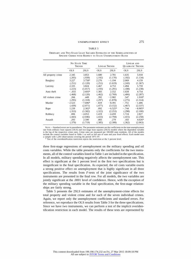
TABLE 6
Ordinary Least Squares Regressions of the Rape Crime Rate on Total and Gender-Specific Unemployment and Employment Rates
A. Unemployment Rate Models
No State Time Trends Linear Trends Linear and Quadratic Trends
(1) (2) (3) (4) (5) (6) (7) (8) (9) (10) (11) (12)
Total unemployment .674 . . . . . . . . . �.305 . . . . . . . . . �.937 . . . . . . . . .(.426) (.418) (.427)
Male unemployment . . . . . . .939 1.652 . . . . . . .042 .407 . . . . . . �.284 .229(.366) (.527) (.346) (.437) (.359) (.426)
Female unemployment . . . .237 . . . �1.184 . . . �.406 . . . �.696 . . . �.914 . . . �1.052(.440) (.630) (.403) (.509) (.397) (.473)
B. Employment Rate Models
No State Time Trends Linear Trends Linear and Quadratic Trends
(1) (2) (3) (4) (5) (6) (7) (8) (9) (10) (11) (12)
Total employment 2.527 . . . . . . . . . 1.353 . . . . . . . . . 1.214 . . . . . . . . .(.433) (.426) (.511)
Male employment . . . . . . �.589 �1.058 . . . . . . �.461 �.672 . . . . . . .009 �.036(.315) (.353) (.279) (.305) (.281) (.310)
Female employment . . . .569 . . . 1.064 . . . .245 . . . .511 � .089 . . . .104(.325) (.363) (.274) (.299) (.269) (.296)
Note.—Standard errors are in parentheses. All regressions include the control variable listed in Table 1 as well as full sets of state and year fixed effects. There are 851observations, and the panel covers the period 1981–97. The dependent variable is the log of the number of rapes per 100,000 state residents.
This content downloaded from 199.190.174.232 on Fri, 27 Mar 2015 18:09:18 PMAll use subject to JSTOR Terms and Conditions

unemployment effect 279
quadratic trends. Again, all of the variables listed in Table 1 are included in allmodels.
Starting with the unemployment models in panel A, the regression in columns(1), (5), and (9) present estimates for the aggregate unemployment rate. Thepattern is similar to the results for the longer time period in Table 3. When thetrends are omitted, there is a positive yet insignificant unemployment effect (.674),adding the linear trends yields a negative insignificant estimate (�.305), whileadding the quadratic trends yields a negative and significant (at 5 percent) estimateof the effect of unemployment on rape (�.937). Columns (2), (6), and (10)present similar models in which the female unemployment rate is substituted forthe aggregate rate. The pattern is quite similar, with insignificant estimates forthe first two specifications and a negative and significant point estimate in column(10) of �.914. Hence, the same pattern exists using the unemployment rate fora nonoffending population. Columns (3), (7), and (11) substitute the male un-employment rate. Here, the first specification yields a positive significant effect,while the second and third specifications yield insignificant effects. The pointestimates for male unemployment are consistently larger than those for the femaleunemployment and total unemployment rates.
Finally, in columns (4), (8), and (12), we add both the male and femaleunemployment rates to the specification. In all three regressions, the coefficienton female unemployment is negative. Moreover, these effects are significant inthe first and third regressions. For male unemployment rates, all coefficient es-timates are positive with a significant effect (at the 1 percent level) in the firstspecification (column (4)). Adding female unemployment rates increases the pointestimate on the male unemployment coefficient in all models. Hence, the resultsfrom panel A yield more sensible findings for rape than those from the previoussection: instead of being unrelated or negatively related to rape, the effects onrape of the unemployment rate of the offending population are generally positiveand sometimes significant.
Panel B presents comparable results when employment rates are substitutedfor unemployment rates. Here, the “correct” sign would be negative. Using theaggregate employment rate in columns (1), (5), and (9), we consistently findemployment effects of the wrong sign. In all specifications, employment exertsa positive and significant effect on rape. Hence, the perverse results are evenstronger using employment rates. In the models that substitute female employ-ment rate for the aggregate rate, there is a weakly significant positive effect inthe first specification and insignificant positive effects in the last two specifi-cations. In contrast, the first two specifications of the model that include maleemployment rates yield only weakly significant negative effects of male em-ployment on rape rates, while in the final specification the point estimate iseffectively zero.
Finally, controlling for both male and female employment rates simultaneouslyyields results similar to the models using the unemployment rates. The coeffi-cients on male employment become larger (more negative) and are significant
This content downloaded from 199.190.174.232 on Fri, 27 Mar 2015 18:09:18 PMAll use subject to JSTOR Terms and Conditions

280 the journal of law and economics
at the 1 and 5 percent levels in the first and second specifications, respectively.In the final specification, the point estimate is still small and insignificant. Finally,for the first two specifications, female employment rates exert positive significanteffects, while in the third specification the variable is insignificant.
In sum, the strategy pursued in this section indicates that the “perverse” un-employment coefficients for some violent offenses are caused by omitted-variables bias. One possible interpretation would be that in good times exposureto offenders is higher, thus masking the negative effect of unemployment on thepropensity to commit violent crimes. In the case of rape, we can show that theemployment prospects of males are weakly related to rape rates. Most important,the results for female unemployment rates indicate that the negative significantunemployment effects observed in Table 3 result from model misspecification.While this strategy cannot be applied to murder rates because of the fact thatthere is not a similarly clear distinction between offenders and victims, the resultsfor rape suggest that a similar fix may yield findings in contrast to those presentedabove.
VI. Conclusion
The results presented here consistently indicate that unemployment is an im-portant determinant of property crime rates. The strong effects on property crimesexist in models of aggregate property crime rates as well as models of theindividual felonies. Moreover, the results for property crimes do not depend onthe estimation methodology used, although we do find relatively stronger effectswhen we instrument for state unemployment rates. Hence, the results of thispaper strongly confirm a basic economic model of the determination of propertycrimes.
We did not find such consistency for violent crimes. In our OLS results, wefind some evidence that the economically motivated violent crime of robbery ispositively affected by unemployment rates. This finding, however, is not repro-duced when we instrument for unemployment. For the crimes of murder andrape, our initial results indicate that unemployment is negatively related to thesecrimes. Upon closer examination of the rape models, however, this paradoxicalresult vanishes. These findings for rape cast doubt on a behavioral interpretationof the observed negative effects on murder—that is to say, being unemployedreduces one’s tendency to become violent and murder someone.
In the opening paragraphs, we cite the recent downward trends in crime oc-curring during the 1990s. To put our results into perspective, it is instructive towork through how much of the recent declines can be explained by the declinein unemployment rates assuming that our estimation results are valid. Sinceour findings for rape indicate that (1) the unemployment effect on rape isweakly positive or insignificant and (2) OLS estimates of the violent crime-unemployment relationship appear to be downwardly biased by omitted factors,we can assume that the unemployment effects on both murder and rape are zero.
This content downloaded from 199.190.174.232 on Fri, 27 Mar 2015 18:09:18 PMAll use subject to JSTOR Terms and Conditions

unemployment effect 281
Moreover, since the estimation results generally indicate that the unemploymenteffect on assault is zero, we also omit this crime rate from these simple simu-lations. To present conservative estimates of the potential contribution of de-clining unemployment, we use the OLS estimates from the most complete modelspecification (Table 3, column 3).
Between 1992 and 1997 (the last 6 years of our panel), the rate of robberydecreased by 30 percent, the rates of auto theft and burglary declined by morethan 15 percent, and larceny declined by slightly more than 4 percent. Concur-rently, the unemployment rate declined from approximately 7.4 to 4.9 percent.Our OLS estimates from the most complete specification predict that the 2.5percentage point decline in unemployment caused a decrease of 5 percent forburglary, 3.7 percent for larceny, 2.5 percent for auto theft, and 4.3 percent forrobbery. Expressed as a percentage of actual declines, our estimates indicate that28 percent for burglary, 82 percent for larceny, 14 percent for auto theft, and14 percent for robbery is attributable to the decline in the unemployment rate.If we look at the overall property crime rate, slightly more than 40 percent ofthe decline can be attributed to the decline in unemployment.
Hence, the magnitudes of the crime-unemployment effects presented here rel-ative to overall movements in crime rates are substantial and suggest that policiesaimed at improving the employment prospects of workers facing the greatestobstacles can be effective tools for combating crime. Moreover, given that crimerates in the United States are considerably higher in areas with high concentrationsof jobless workers (many inner-city communities, for example) and the fact thatthose workers with arguably the worst employment prospects (young African-American males) are the most likely to be involved with the criminal justicesystem, employment-based anticrime policies contain the attractive feature ofbeing consistent with a wide range of policy objectives.
Bibliography
Blanchard, Olivier Jean, and Katz, Lawrence F. “Regional Evolutions.” BrookingsPapers on Economic Activity, no. 1 (1992): 1–75.
Bound, John, and Freeman, Richard B. “What Went Wrong? The Erosion ofRelative Earnings and Employment among Young Black Men in the 1980s.”Quarterly Journal of Economics 107 (1992): 201–32.
Boyum, David A., and Kleiman, Mark A. R. “Alcohol and Other Drugs.” InCrime, edited by James Q. Wilson and Joan Petersilia, pp. 295–326. SanFrancisco: ICS Press, 1995.
Bushway, Shawn, and Engberg, John. “Panel Data VAR Analysis of theRelationship between Crime and Unemployment.” Working paper. Pittsburgh:Carnegie Mellon University, 1994.
Chiricos, Theodor. “Rates of Crime and Unemployment: An Analysis ofAggregate Research Evidence.” Social Problems 34 (1987): 187–212.
This content downloaded from 199.190.174.232 on Fri, 27 Mar 2015 18:09:18 PMAll use subject to JSTOR Terms and Conditions

282 the journal of law and economics
Cook, Philip J., and Moore, Mark H. “Gun Control.” In Crime, edited by JamesQ. Wilson and Joan Petersilia, pp. 267–94. San Francisco: ICS Press, 1995.
Cook, Philip J., and Zarkin, Gary A. “Crime and the Business Cycle.” Journalof Legal Studies 14 (1985): 115–28.
Corman, Hope; Joyce, Theodor; and, Lovitch, Norman. “Crime, Deterrence andthe Business Cycle in New York City: A VAR Approach.” Review ofEconomics and Statistics 69 (1987): 695–700.
Corman, Hope, and Mocan, H. Naci. “A Time-Series Analysis of Crime,Deterrence and Drug Abuse in New York City.” American Economic Review90 (2000): 584–604.
Davis, Steven J.; Loungani, Prakash; and Malidhara, Ramamohan. “RegionalLabor Fluctuations: Oil Shocks, Military Spending, and other Driving Forces.”IF Working Paper No. 578. Washington, D.C.: Board of Governors of theFederal Reserve System, 1997.
Entorf, Horst, and Spengler, Hannes. “Socioeconomic and Demographic Factorsof Crime in Germany: Evidence from Panel Data of the German States.”International Review of Law and Economics 20 (2000): 75–106.
Fagan, Jeffrey. “Intoxication and Aggression.” In Drugs and Crime, ed. MichaelH. Tonry and James Q. Wilson, pp. 241–320. Volume 13 of Crime and Justice:A Review of Research. Chicago: University of Chicago Press, 1990.
Freeman, Scott; Grogger, Jeffrey; and Sonstelie, Jon. “The Spatial Concentrationof Crime.” Journal of Urban Economics 40 (1996): 216–31.
Friedberg, Leora. “Did Unilateral Divorce Raise Divorce Rates? Evidence fromPanel Data.” American Economic Review 88 (1998): 608–27.
Gould, Eric D.; Weinberg, Bruce A.; and Mustard, David B. “Crime Rates andLocal Labor Market Opportunities in the United States: 1977–1997.” Reviewof Economics and Statistics, forthcoming, 2001.
Greenberg, David F. “Age, Crime, and Social Explanation.” American Journalof Sociology 91 (1985): 1–21.
Greenberg, Edward. “Employment Impacts of Defense Expenditures andObligations.” Review of Economics and Statistics 49 (1967): 186–98.
Grogger, Jeffrey. “The Effect of Arrests on the Employment and Earnings ofYoung Men.” Quarterly Journal of Economics 110 (1995): 51–71.
Grogger, Jeff. “Market Wages and Youth Crime.” Journal of Labor Economics16 (1998): 756–91.
Hirshi, Travis, and Gottfredson, Michael. “Age and the Explanation of Crime.”American Journal of Sociology 89 (1983): 552–84.
Hooker, Mark A., and Knetter, Michael M. “Unemployment Effects of MilitarySpending: Evidence from a Panel of States.” Working Paper No. 4889.Cambridge, Mass.: National Bureau of Economic Research, 1994.
Hooker, Mark A., and Knetter, Michael M. “The Effects of Military Spendingon Economic Activity: Evidence from State Procurement Spending.” Journalof Money, Credit and Banking 28 (1997): 400–421.
Levitt, Steven D. “The Effect of Prison Population Size on Crime Rates: Evidence
This content downloaded from 199.190.174.232 on Fri, 27 Mar 2015 18:09:18 PMAll use subject to JSTOR Terms and Conditions

unemployment effect 283
from Prison Overcrowding Litigation.” Quarterly Journal of Economics 111(1996): 319–51.
Levitt, Steven D. “Using Electoral Cycles in Police Hiring to Estimate the Effectof Police on Crime.” American Economic Review 87 (1997): 270–90.
Marvell, Thomas B., and Moody, Carlisle E. “The Impact of Enhanced PrisonTerms for Felonies Committed with Guns.” Criminology 33 (1995): 247–49.
Marvell, Thomas B., and Moody, Carlisle E. “Determinate Sentencing andAbolishing Parole: The Long-Term Impacts on Prisons and Crime.”Criminology 34 (1996): 107–28.
Mayer, Kenneth R. The Political Economy of Defense Contracting. New Haven,Conn.: Yale University Press, 1991.
Nagin, Daniel, and Waldfogel, Joel. “The Effects of Criminality and Convictionon the Labor Market Status of Young British Offenders.” International Reviewof Law and Economics 15 (1995): 109–26.
Papps, Kerry, and Winkelmann, Rainer. “Unemployment and Crime: NewAnswers to an Old Question.” Working paper. New Zealand: University ofCanterbury, 1998.
Rennison, Callie M. “Criminal Victimization 1998: Changes 1997–1998 withTrends 1993–1998.” Report No. NCJ-1766353. Washington, D.C.: U.S.Department of Justice, 1999.
Ruhm, Christopher J. “Economic Conditions and Alcohol Problems.” Journalof Health Economics 14 (1995): 583–603.
U. S. Department of Justice. “Sex Offenses and Offenders: An Analysis of Dataon Rape and Sexual Assault.” Report No. NCJ-163392. Washington, D.C.:U.S. Department of Justice, Bureau of Justice Statistics, 1997.
Willis, Michael. “Crime and the Location of Jobs.” Working paper. Santa Barbara:University of California, Santa Barbara, 1999.
Willis, Michael. “Unemployment, the Minimum Wage, and Crime.” Workingpaper. Santa Barbara: University of California, Santa Barbara, 1999.
Witte, Ann Dryden, and Tauchen, Helen. “Work and Crime: An ExplorationUsing Panel Data.” Working Paper No. 4794. Cambridge, Mass.: NationalBureau of Economic Research, 1994.
This content downloaded from 199.190.174.232 on Fri, 27 Mar 2015 18:09:18 PMAll use subject to JSTOR Terms and Conditions