Embed Size (px)
Citation preview

I
A
bc�dc2ma22fimMve
e
©
GEOPHYSICS, VOL. 72, NO. 2 �MARCH-APRIL 2007�; P. S123–S132, 14 FIGS.10.1190/1.2434780
dentification of image artifacts from internal multiples
lison E. Malcolm1, Maarten V. de Hoop2, and Henri Calandra3
tattmtptttItoti
ABSTRACT
First-order internal multiples are a source of coherent noise inseismic images because they do not satisfy the single-scatteringassumption fundamental to most seismic processing. There are anumber of techniques to estimate internal multiples in data; inmany cases, these algorithms leave some residual multiple ener-gy in the data. This energy produces artifacts in the image, andthe location of these artifacts is unknown because the multipleswere estimated in the data before the image was formed. To avoidthis problem, we propose a method by which the artifacts causedby internal multiples are estimated directly in the image. We useideas from the generalized Bremmer series and the Lippmann-Schwinger scattering series to create a forward-scattering seriesto model multiples and an inverse-scattering series to describe
ic
tfdieVamhpmefl
eived On, Colo
est La
S123
he impact these multiples have on the common-image gathernd the image. We present an algorithm that implements the thirderm of this series, responsible for the formation of first-order in-ernal multiples. The algorithm works as part of a wave-equation
igration; the multiple estimation is made at each depth using aechnique related to one used to estimate surface-related multi-les. This method requires knowledge of the velocity model tohe depth of the shallowest reflector involved in the generation ofhe multiple of interest. This information allows us to estimate in-ernal multiples without assumptions inherent to other methods.n particular, we account for the formation of caustics. Results ofhe techniques on synthetic data illustrate the kinematic accuracyf predicted multiples, and results on field data illustrate the po-ential of estimating artifacts caused by internal multiples in themage rather than in the data.
INTRODUCTION
That internal multiples are present in seismic experiments haseen acknowledged for a long time �Sloat, 1948�. At present, signifi-antly more is known about attenuation of surface-related multiplesAnstey and Newman, 1966; Kennett, 1974; Aminzadeh and Men-el, 1980; Fokkema and van den Berg, 1993; Berkhout and Vers-huur, 1997; Verschuur and Berkhout, 1997; Weglein et al., 1997,003� than is known about attenuation of internal multiples �Fokke-a et al., 1994; Weglein et al., 1997; Jakubowicz, 1998; Kelamis et
l., 2002; ten Kroode, 2002; van Borselen, 2002; Weglein et al.,003; Berkhout and Verschuur, 2005; Verschuur and Berkhout,005�. With the exception of techniques such as the angle-domainltering proposed by Sava and Guitton �2005� and the image-do-ain surface-related multiple prediction technique of Artman andatson �2006�, the current state of the art in multiple attenuation in-
olves estimating multiples in the data. We propose an algorithm forstimating imaging artifacts caused by internal multiples directly on
Manuscript received by the Editor March 20, 2006; revised manuscript rec1Formerly Center for Wave Phenomena, Colorado School of Mines, Golde
rlands. E-mail: [email protected] University, Center for Computational and Applied Mathematics, W3Total E & P, Pau, France. E-mail: [email protected] Society of Exploration Geophysicists. All rights reserved.
mage gathers and images, as part of a wave-equation imaging pro-edure of the downward continuation type.
Fokkema and van den Berg �1993� used reciprocity, along withhe representation theorem, to show that it is possible to predict sur-ace-related multiples from seismic reflection data and that this pre-iction can be carried out through a Neumann series expansion. Thisdea is fundamental to surface-related �SRME� and internal multiplestimation techniques of Berkhout and Verschuur �Berkhout anderschuur, 1997, 2005; Verschuur and Berkhout, 1997, 2005�; other
uthors have also built upon these ideas �Fokkema et al., 1994; Kela-is et al., 2002; van Borselen, 2002�. The technique discussed here
as its roots in these ideas but differs from other methods because weropose estimating, directly in the image, artifacts caused by internalultiples �IM�. This approach is in contrast to previous methods that
stimate IM and subtract them from the data before an image isormed. We develop and test our method specifically for first- oreading-order internal multiples, but the extension to higher orders is
ctober 4, 2006; published online March 2, 2007.rado; presently Utrecht University, Department of Earth Sciences, the Neth-
fayette, Indiana. E-mail: [email protected].
sbrp
�tithfttp�tc�acttttfc�ie
mcceasmetttss
v1auigrh
nHtofbmaatkivdd2hr
sSbpmwmmwaorl
stugAmF
rd̃srmct
FTs
S124 Malcolm et al.
traightforward. The series used to estimate image artifacts causedy IM is a hybrid between the Lippmann-Schwinger scattering se-ies used by Weglein et al. �1997� and the generalized Bremmer cou-ling series, a Neumann series, introduced by de Hoop �1996�.
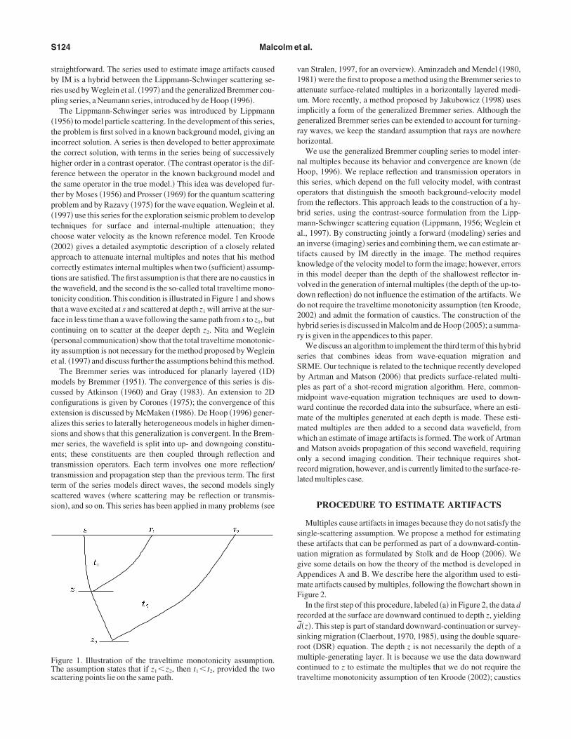
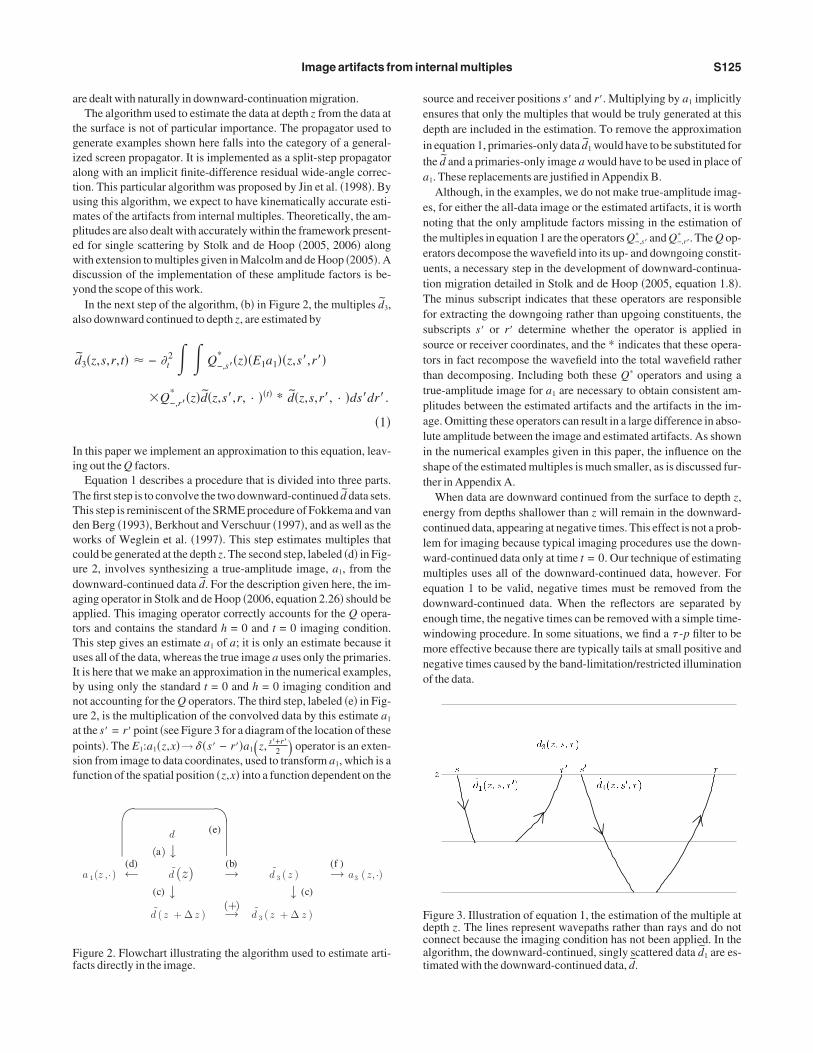
The Lippmann-Schwinger series was introduced by Lippmann1956� to model particle scattering. In the development of this series,he problem is first solved in a known background model, giving anncorrect solution. A series is then developed to better approximatehe correct solution, with terms in the series being of successivelyigher order in a contrast operator. �The contrast operator is the dif-erence between the operator in the known background model andhe same operator in the true model.� This idea was developed fur-her by Moses �1956� and Prosser �1969� for the quantum scatteringroblem and by Razavy �1975� for the wave equation. Weglein et al.1997� use this series for the exploration seismic problem to developechniques for surface and internal-multiple attenuation; theyhoose water velocity as the known reference model. Ten Kroode2002� gives a detailed asymptotic description of a closely relatedpproach to attenuate internal multiples and notes that his methodorrectly estimates internal multiples when two �sufficient� assump-ions are satisfied. The first assumption is that there are no caustics inhe wavefield, and the second is the so-called total traveltime mono-onicity condition. This condition is illustrated in Figure 1 and showshat a wave excited at s and scattered at depth z1 will arrive at the sur-ace in less time than a wave following the same path from s to z1, butontinuing on to scatter at the deeper depth z2. Nita and Wegleinpersonal communication� show that the total traveltime monotonic-ty assumption is not necessary for the method proposed by Wegleint al. �1997� and discuss further the assumptions behind this method.
The Bremmer series was introduced for planarly layered �1D�odels by Bremmer �1951�. The convergence of this series is dis-
ussed by Atkinson �1960� and Gray �1983�. An extension to 2Donfigurations is given by Corones �1975�; the convergence of thisxtension is discussed by McMaken �1986�. De Hoop �1996� gener-lizes this series to laterally heterogeneous models in higher dimen-ions and shows that this generalization is convergent. In the Brem-er series, the wavefield is split into up- and downgoing constitu-
nts; these constituents are then coupled through reflection andransmission operators. Each term involves one more reflection/ransmission and propagation step than the previous term. The firsterm of the series models direct waves, the second models singlycattered waves �where scattering may be reflection or transmis-ion�, and so on. This series has been applied in many problems �see
igure 1. Illustration of the traveltime monotonicity assumption.he assumption states that if z1 �z2, then t1 � t2, provided the twocattering points lie on the same path.
an Stralen, 1997, for an overview�. Aminzadeh and Mendel �1980,981� were the first to propose a method using the Bremmer series tottenuate surface-related multiples in a horizontally layered medi-m. More recently, a method proposed by Jakubowicz �1998� usesmplicitly a form of the generalized Bremmer series. Although theeneralized Bremmer series can be extended to account for turning-ay waves, we keep the standard assumption that rays are nowhereorizontal.
We use the generalized Bremmer coupling series to model inter-al multiples because its behavior and convergence are known �deoop, 1996�. We replace reflection and transmission operators in
his series, which depend on the full velocity model, with contrastperators that distinguish the smooth background-velocity modelrom the reflectors. This approach leads to the construction of a hy-rid series, using the contrast-source formulation from the Lipp-ann-Schwinger scattering equation �Lippmann, 1956; Weglein et
l., 1997�. By constructing jointly a forward �modeling� series andn inverse �imaging� series and combining them, we can estimate ar-ifacts caused by IM directly in the image. The method requiresnowledge of the velocity model to form the image; however, errorsn this model deeper than the depth of the shallowest reflector in-olved in the generation of internal multiples �the depth of the up-to-own reflection� do not influence the estimation of the artifacts. Weo not require the traveltime monotonicity assumption �ten Kroode,002� and admit the formation of caustics. The construction of theybrid series is discussed in Malcolm and de Hoop �2005�; a summa-y is given in the appendices to this paper.
We discuss an algorithm to implement the third term of this hybrideries that combines ideas from wave-equation migration andRME. Our technique is related to the technique recently developedy Artman and Matson �2006� that predicts surface-related multi-les as part of a shot-record migration algorithm. Here, common-idpoint wave-equation migration techniques are used to down-ard continue the recorded data into the subsurface, where an esti-ate of the multiples generated at each depth is made. These esti-ated multiples are then added to a second data wavefield, fromhich an estimate of image artifacts is formed. The work of Artman
nd Matson avoids propagation of this second wavefield, requiringnly a second imaging condition. Their technique requires shot-ecord migration, however, and is currently limited to the surface-re-ated multiples case.
PROCEDURE TO ESTIMATE ARTIFACTS
Multiples cause artifacts in images because they do not satisfy theingle-scattering assumption. We propose a method for estimatinghese artifacts that can be performed as part of a downward-contin-ation migration as formulated by Stolk and de Hoop �2006�. Weive some details on how the theory of the method is developed inppendices A and B. We describe here the algorithm used to esti-ate artifacts caused by multiples, following the flowchart shown inigure 2.In the first step of this procedure, labeled �a� in Figure 2, the data d
ecorded at the surface are downward continued to depth z, yielding�z�. This step is part of standard downward-continuation or survey-inking migration �Claerbout, 1970, 1985�, using the double square-oot �DSR� equation. The depth z is not necessarily the depth of aultiple-generating layer. It is because we use the data downward
ontinued to z to estimate the multiples that we do not require theraveltime monotonicity assumption of ten Kroode �2002�; caustics
a
tgiatumpewdy
a
Ii
TTdwcudaatTuIbnuapsf
sedita
enteutTfsstttpalist
eclwmedewmno
Ff
Fdcat
Image artifacts from internal multiples S125
re dealt with naturally in downward-continuation migration.The algorithm used to estimate the data at depth z from the data at
he surface is not of particular importance. The propagator used toenerate examples shown here falls into the category of a general-zed screen propagator. It is implemented as a split-step propagatorlong with an implicit finite-difference residual wide-angle correc-ion. This particular algorithm was proposed by Jin et al. �1998�. Bysing this algorithm, we expect to have kinematically accurate esti-ates of the artifacts from internal multiples. Theoretically, the am-
litudes are also dealt with accurately within the framework present-d for single scattering by Stolk and de Hoop �2005, 2006� alongith extension to multiples given in Malcolm and de Hoop �2005�. Aiscussion of the implementation of these amplitude factors is be-ond the scope of this work.
In the next step of the algorithm, �b� in Figure 2, the multiples d̃3,lso downward continued to depth z, are estimated by
d̃3�z,s,r,t� � − �t2 � � Q−,s�
* �z��E1a1��z,s�,r��
�Q−,r�* �z�d̃�z,s�,r, · ��t� * d̃�z,s,r�, · �ds�dr�.
�1�
n this paper we implement an approximation to this equation, leav-ng out the Q factors.
Equation 1 describes a procedure that is divided into three parts.he first step is to convolve the two downward-continued d̃ data sets.his step is reminiscent of the SRME procedure of Fokkema and vanen Berg �1993�, Berkhout and Verschuur �1997�, and as well as theorks of Weglein et al. �1997�. This step estimates multiples that
ould be generated at the depth z. The second step, labeled �d� in Fig-re 2, involves synthesizing a true-amplitude image, a1, from theownward-continued data d̃. For the description given here, the im-ging operator in Stolk and de Hoop �2006, equation 2.26� should bepplied. This imaging operator correctly accounts for the Q opera-ors and contains the standard h = 0 and t = 0 imaging condition.his step gives an estimate a1 of a; it is only an estimate because itses all of the data, whereas the true image a uses only the primaries.t is here that we make an approximation in the numerical examples,y using only the standard t = 0 and h = 0 imaging condition andot accounting for the Q operators. The third step, labeled �e� in Fig-re 2, is the multiplication of the convolved data by this estimate a1
t the s� = r� point �see Figure 3 for a diagram of the location of theseoints�. The E1:a1�z,x�→� �s� − r��a1�z, s�+r�
2 � operator is an exten-ion from image to data coordinates, used to transform a1, which is aunction of the spatial position �z,x� into a function dependent on the
d
(a) ↓a 1 ( z , )
(d)← d̃ ( z )(b)→ d̃ 3 ( z )
(f )→ a3 ( z,.)
(c) ↓ ↓ (c)d̃ ( z + ∆ z )
(+)→ d̃ 3 ( z + ∆ z )
(e)
.
igure 2. Flowchart illustrating the algorithm used to estimate arti-acts directly in the image.
ource and receiver positions s� and r�. Multiplying by a1 implicitlynsures that only the multiples that would be truly generated at thisepth are included in the estimation. To remove the approximationn equation 1, primaries-only data d̃1 would have to be substituted forhe d̃ and a primaries-only image a would have to be used in place of
1. These replacements are justified in Appendix B.Although, in the examples, we do not make true-amplitude imag-
s, for either the all-data image or the estimated artifacts, it is worthoting that the only amplitude factors missing in the estimation ofhe multiples in equation 1 are the operators Q−,s�
* and Q−,r�* . The Q op-
rators decompose the wavefield into its up- and downgoing constit-ents, a necessary step in the development of downward-continua-ion migration detailed in Stolk and de Hoop �2005, equation 1.8�.he minus subscript indicates that these operators are responsible
or extracting the downgoing rather than upgoing constituents, theubscripts s� or r� determine whether the operator is applied inource or receiver coordinates, and the * indicates that these opera-ors in fact recompose the wavefield into the total wavefield ratherhan decomposing. Including both these Q* operators and using arue-amplitude image for a1 are necessary to obtain consistent am-litudes between the estimated artifacts and the artifacts in the im-ge. Omitting these operators can result in a large difference in abso-ute amplitude between the image and estimated artifacts. As shownn the numerical examples given in this paper, the influence on thehape of the estimated multiples is much smaller, as is discussed fur-her in Appendix A.
When data are downward continued from the surface to depth z,nergy from depths shallower than z will remain in the downward-ontinued data, appearing at negative times. This effect is not a prob-em for imaging because typical imaging procedures use the down-ard-continued data only at time t = 0. Our technique of estimatingultiples uses all of the downward-continued data, however. For
quation 1 to be valid, negative times must be removed from theownward-continued data. When the reflectors are separated bynough time, the negative times can be removed with a simple time-indowing procedure. In some situations, we find a � -p filter to beore effective because there are typically tails at small positive and
egative times caused by the band-limitation/restricted illuminationf the data.
igure 3. Illustration of equation 1, the estimation of the multiple atepth z. The lines represent wavepaths rather than rays and do notonnect because the imaging condition has not been applied. In thelgorithm, the downward-continued, singly scattered data d̃1 are es-imated with the downward-continued data, d̃.

iFitctt
tmwit
cicvdco
tFbp
dmtocet
cpbdicbotF
F
ficpi�ft
sFgr
Ffirlmt
Fm
S126 Malcolm et al.
To compare the artifacts in the image with estimated artifacts, anmage must also be formed with the estimated multiples; this is �f� inigure 2. This image, denoted a3, is formed in the manner discussed
n �b� of Figure 2. It is interesting to note that the agreement betweenhe image artifacts and the estimated artifacts does not depend on thehoice of velocity model below the depth of the up-to-down reflec-ion �z in Figure 3� because the true and estimated multiples will seehe same error.
This procedure completes one depth step of the algorithm. Afterhe above tasks are complete, both the wavefield and the estimate
ultiples are downward continued to the next depth level, z + �z,hich is step �c� in Figure 2. At this depth step, the entire procedure
s repeated with the multiples estimated at this new depth added tohe downward-continued multiples from the previous depth.
In equation 1, two data sets, each containing a source wavelet, areonvolved together to estimate the multiples. As in other techniquesn which multiples are estimated through such a convolution, an ac-urate estimate requires that one copy of this wavelet be decon-olved from the estimated multiples. In addition, as the data areownward continued into the subsurface, the range of data offsetsontaining significant energy will become narrower. That narrowffsets will be available is advantageous for multiple prediction, but
Tim
e (s
)
–2
0
2
4
–0.8 0 0.8Offset (km)
Tim
e (s
)
–2
0
2
4
–0.8 0 0.8Offset (km)
a) b)
igure 4. �a� Data downward continued to 1.5 km, the depth of therst reflector. The curve shows the expected moveout for the �prima-y� reflection from the bottom of the layer, and the vertical lines de-ineate the expected illumination of this reflection. �b� The estimated
ultiple, in the data, at a depth of 1.5 km; note the agreement withhe true multiple in �a�.
he lack of larger offsets may be detrimental in some situations.urther, to obtain accurate amplitude estimates, corrections shoulde made for differences in illumination between multiples andrimaries.
EXAMPLES
In this section, we describe the results of applying the technique toata. Three different synthetic models are presented. A flat-layeredodel illustrates the steps of the algorithm. Following this descrip-
ion, a more complicated model is used to test the ability of the meth-d to estimate imaging artifacts caused by IM in the presence ofaustics and to test the sensitivity of the method to the velocity mod-l. We also present a field-data example, consisting of a 2D line ex-racted from a 3D survey in the Gulf of Mexico.
The displayed images, for both a1 and a3, have had automatic gainontrol �AGC� applied to enhance the multiple contribution. Com-utational artifacts such as Fourier wrap-around and computationaloundary effects were suppressed, but not fully eliminated, in theownward continuation by padding with zeros and tapering the datan both midpoint and offset. In most figures, the true reflectors arelipped to show artifacts more clearly. Although the wavelet has noteen deconvolved, the data have been shifted in time so that the peakf the source wavelet is at zero time and bandpass filtered to matchhe frequency content of the two images. The synthetic examples inigures 4–11 are shown with an aspect ratio of 1/4.
lat model
The model in the first example consists of a single layer, extendingrom 1.5 to 2.5 km, with a velocity of 2 km/s; the layer is embeddedn a homogeneous model with velocity 6 km/s. Synthetic data wereomputed in this model with finite-difference modeling; 101 mid-oints were generated with 101 offsets at each midpoint and a spac-ng of 15 m in both midpoint and offset �we define offset asr − s�/2�; 4 s of data were computed at 4-ms sampling, with a peakrequency of 10 Hz and a maximum frequency of 20 Hz. To imagehese data, a depth step of 10 m was used.
In our method, the data are first downward continued as part of atandard wave-equation migration technique, i.e., �a� in Figure 2. Inigure 4a, we show d̃�z = 1.5 km�, a downward-continued CMPather at the depth z = 1.5 km from the top of the layer. The primaryeflected from the top of the layer is located around t = 0, the reflec-
Dep
th (
km)
0
2
4
6
8
1.51.00.50Midpoint (km)
Dep
th (
km)
0
2
4
6
8
1.51.00.50
a) b)
6 km/s
2 km/s
Midpoint (km)υ
igure 5. �a� The image with an artifact from a first-order internalultiple at about 5.7-km depth. �b� The estimated artifact.

td
emct�tdtmidgoadc
cFbafttF
if
L
mmlt−eTbseiw
vaictt9ttb
t
p1dmtsclm
Fcom
Fotm
Image artifacts from internal multiples S127
ion from the bottom of the layer is at about t = 1 s, and the first-or-er internal multiple is at about t = 2 s.
We now estimate the multiples at depth by using equation 1. Thisstimation requires restricting d̃ to time t � 0. The procedure re-oves the primary reflection from the current depth �which theoreti-
ally arrives at t = 0�, in this case 1.5 km, before doing the convolu-ion. If this process is not done correctly and energy remains at t
0, all primary reflections from deeper depths will be duplicated inhe estimated-multiples section. In this model, a simple time-win-owing procedure is sufficient because the reflections are far apart inime. Once the negative time contributions to the data have been re-
oved, the data are convolved to estimate the multiple. The result-ng wavefield is multiplied by an estimate of the image at the currentepth �this is the �E1a1��z,s�,r�� term appearing in equation 1� toive the estimate in Figure 4b. The event at about t = 3 s is a second-rder internal multiple. This event is formed from the convolution ofprimary with a first-order internal multiple. It is not present in theata panel because later arrivals were muted. These calculationsomplete step �b� in Figure 2.
We now proceed to �c� of the flowchart in Figure 2 and downwardontinue both the data and the estimated multiples to the next depth.rom the data, an image at the current depth is formed containingoth primaries and multiples, i.e., �d� in Figure 2. Another image islso computed at the current depth, containing an estimate of the arti-acts caused by leading-order IM, i.e., �f� in Figure 2. The image con-aining both primaries and multiples gives the estimate a1�z,x�hat feeds back into the estimation of the multiples through �e� ofigure 2.Figure 5 compares the estimated artifact a3 �Figure 5b� with the
maged data a1 �Figure 5a�. The estimated artifact overlays the arti-act in the primary image.
ens model
To illustrate the ability of the method to estimate multiples inore complicated velocity models, we add a low-velocity lens to theodel. The resulting velocity model is shown in Figure 6. The lens is
ocated in the center of the model; it is circular with Gaussian veloci-y variations, a diameter of 600 m, and a maximum contrast of2 km/s. The addition of the lens has a large influence on the record-d data. The data from a midpoint of 9.8 km are shown in Figure 7.he first arrival is enlarged in Figure 7b to show the caustics causedy the lens more clearly. The estimated multiples in the image arehown in Figure 8. Once again, the multiple is relatively weak in thestimated image, because of the residual moveout on the common-mage gathers, which are also shown in Figure 8. The image gathersere computed by using the method of Prucha et al. �1999�.To illustrate the dependence of this method on the background-
elocity model, we now test the sensitivity of the estimated multiplertifact to errors in the velocity. In theory, knowledge of the velocitys necessary only to the depth of the shallowest reflection; in thisase, the top of the layer at 2-km depth. To test this concept, we per-urb the model by adding a second lens, with properties identical tohe first lens, below the layer. The estimated artifact, shown in Figure, still matches the image artifact quite well. The tail on the far left ofhe image is likely the result of Fourier wrap-around in the propaga-or; other differences likely come from differences in illuminationetween estimated and true multiples.
To test the sensitivity of the method to errors in the velocity abovehe layer, we remove the lens and estimate the image and the multi-
le in this incorrect velocity model. The results are shown in Figure0. Although the estimated artifact remains at roughly the correctepth, the variation in the image with midpoint is not accurately esti-ated. Removing the lens entirely is a large change in the model;
hus, we expect a large change in the image. In Figure 11, we demon-trate that we can still estimate the multiple with reasonable accura-y when the velocity perturbation is less dramatic. In this case, theens has been moved 0.2 km shallower than in the true-velocity
odel, and the result is still acceptable.
Dep
th (
km)
0
2
4
6
8
10.510.09.59.0
Midpoint (km)
igure 6. Velocity model, similar to the flat-layered example dis-ussed previously, with the addition of a low-velocity lens to dem-nstrate that the method works in laterally heterogeneous velocityodels.
Tim
e (s
)
0
2
4
–1 0 1
Offset (km)
Tim
e (s
)
0.5
1.0
–1 0 1
Offset (km)a) b)
igure 7. Common-midpoint gather at 9.8 km and zero depth, withnly the offsets used to compute the images shown later. Note theriplications caused by the lens. �a� Full gather. �b� Zoom of the pri-
ary reflection from the top layer.

F
dsbsetsslfDiw
cmi
a
F6s
a
Flswfi
a
Fgop�m
a
FttIe
S128 Malcolm et al.
ield data
We present an example of the application of this method to fieldata. The data are from the Gulf of Mexico in a region with a largealt body. Estimating internal multiples in such an area is difficultecause of multipathing introduced by the salt. The data have hadtandard preprocessing applied, including surface-related multiplelimination and a Radon demultiple; they have also been regularizedo a uniform grid in the midpoint-offset coordinates. We show re-ults from a single 2D line extracted from a 3D survey. Because thealt has a complicated 3D geometry, performing 2D imaging on thisine is likely to introduce errors. Comparison with the image from aull 3D migration indicates that these effects are not overwhelming.espite this, the estimated artifacts are likely to contain errors result-
ng from applying a 2D multiple-estimation algorithm in an areahere the geology is 3D.An image of the line is shown in Figure 12; the base of salt is indi-
ated with the white arrows. The circled regions contain events,arked by black arrows, that are suspected to be artifacts caused by
nternal multiples. To compare the estimated artifacts with the arti-
Dep
th (
km)
0
2
4
6
8
Dep
th (
km)
0
2
4
6
8
10.5 0.05010.09.59.0Midpoint (km) -horizontal (s/km)c) d) p
an artifact from the first-order internal multiple at approximatelyles. �d� Image gather of estimated artifact. The label p-horizontal
Dep
th (
km)
0
2
4
6
8
10.510.09.59.010.510.09.59.0
Midpoint (km)
Dep
th (
km)
0
2
4
6
8
Midpoint (km)) b)
igure 11. In this model, the lens was moved 0.2 km deeper than inhe correct velocity model. Because this perturbation is above theop of the layer, we expect an effect on the estimated multiple. �a�mage with artifacts from first-order internal multiples. �b� Estimat-d artifacts from first-order internal multiples.
Dep
th (
km)
0
2
4
6
8
10.510.09.59.0Midpoint (km)
Dep
th (
km)
0
2
4
6
8
0.050-horizontal (s/km)) b)p
igure 8. �a� Common-image gather for midpoint 9.8 km. �b� Image withkm depth. �c� Image of estimated artifacts from first-order internal multip
tands for the horizontal slowness.
Dep
th (
km)
0
2
4
6
8
10.510.09.59.0
Midpoint (km)
10.510.09.59.0
Midpoint (km)
Dep
th (
km)
0
2
4
6
8
) b)
igure 9. In these images, a second lens has been added beneath theayer to introduce a laterally varying velocity perturbation; thishould not influence the accuracy of the estimated artifact. �a� Imageith artifacts from internal multiples. �b� Estimated artifacts fromrst-order internal multiples.
Dep
th (
km)
0
2
4
6
8
10.510.09.59.010.510.09.59.0
Midpoint (km)
Dep
th (
km)
0
2
4
6
8
Midpoint (km)) b)
igure 10. The lens was removed from the velocity model beforeenerating these images. Because this perturbation is above the topf the layer, we expect this to have an impact on the estimated multi-le. Note the change in the accuracy of the estimate beneath the lens.a� Image with artifacts from first-order internal multiples. �b� Esti-ated artifacts from first-order internal multiples.

fta
meahewmtpn
F
tcraebaresa
�gmtewgls
ckgmcsmt
Fmettramr3
0
a
F�Tctss
0
a
F�Tctaotcha
Image artifacts from internal multiples S129
acts seen in the image space, we show common-image gathers fromwo points in the model, marked by the black arrows beneath the im-ge, covering the three highlighted areas.
The first image gather, shown in Figure 13, is approximately in theiddle of the left highlighted region in Figure 12. There are five ar-
as marked on this image gather at which artifacts are estimated andlso occur in the imaged data. Arrow 4 marks the artifact in the leftighlighted region of the image in Figure 12, indicating that thisvent is indeed an artifact caused by first-order internal multiplesithin the salt body. Arrow 1 marks a number of estimated artifactsixed with primaries within and above the salt. It is possible that
hese artifacts are in fact residual energy from t � 0 that was incom-letely removed. Arrow numbers 2, 3, and 5 indicate plausible inter-al multiples.
The second image gather, shown in Figure 14, is at CMP 600, inigure 12 within the two highlighted regions on the right. First, note
0 100 200 300 400 500 600 700 800
Dep
th (
km)
Midpoint (km)
igure 12. Image for the field-data example. The base of salt isarked with white arrows, and the circles mark three areas of inter-
st, two of which contain artifacts from internal multiples �left andop right� and one of which does not �bottom right�. The locations ofhe CIGs shown in Figures 13 and 14 are marked with the black ar-ows below the image. The depth could not be displayed on this im-ge; to tie the depth in Figure 13, the black arrow on the left imagearks the artifact that arrow 4 points to in Figure 13 and the black ar-
ow on the right of the image points to the position marked by arrowin Figure 14.
Depth
1
2
3
4
5
0.150.100.050
p-horizontal (s/km)
00.050.10.15
p-horizontal (s/km)) b)
0 0
igure 13. Field-data example, common-image gather at CMP 150left black arrow in Figure 12�. �a� The standard image gather. �b�he estimated artifacts from internal multiples. The five arrows indi-ate the locations of accurately estimated artifacts. Arrow 4 is the ar-ifact marked with an arrow in the highlighted region on the imagehown in Figure 12. The label p-horizontal stands for the horizontallowness. The depth could not be displayed on these images.
hat arrow 3 indicates a strong event in the image gather that does notorrespond to an estimated artifact. This is the event in the lower-ight highlighted region of Figure 12 �marked by a black arrow�. Thebsence of an estimated artifact at this position indicates that this en-rgy is not an imaging artifact caused by internal multiples. It coulde, for example, a primary that is migrated poorly resulting from in-ccuracies in the velocity model, or residual energy from a surface-elated multiple, or an out-of-plane effect. Arrows 1 and 2 mark oth-r estimated artifacts in this image gather. Arrow 2 is in the second,hallower highlighted region of Figure 12, indicating that in thisrea, some of the energy does come from internal multiples.
In the common-image gathers, there are many estimated artifactsFigure 14b� that are not easily correlated with events in the imageather made from the full data set �Figure 14a�. Some of these esti-ated artifacts could have been attenuated by the Radon demultiple
hat has been applied to the data. Other sources of error include 3Dffects, both in the image and in the estimation of the multiples, asell as amplitude errors in the estimated artifacts resulting in stron-er amplitudes on the estimated artifacts than on the artifacts actual-y seen in the migration. This example is only intended to demon-trate the potential of the method.
CONCLUSION
We have described a method of estimating imaging artifactsaused by first-order internal multiples. This method requiresnowledge of the velocity model down to the top of the layer thatenerates the multiple �the depth of the up-to-down reflection�. Theain computational cost of the algorithm comes from the downward
ontinuation of the data and the internal multiples. Because two dataets are downward continued �the data themselves and the estimatedultiples�, the cost of the algorithm described here is about twice
hat of a usual prestack depth migration, plus the cost of the removal
Depth
1
2
3
0.150.100.050
p-horizontal (s/km)
00 0
0.050.10.15
p-horizontal (s/km)) b)
igure 14. Field-data example, common-image gather at CMP 600right black arrow in Figure 12�. �a� The standard image gather. �b�he estimated artifacts from internal multiples. Arrows 1 and 2 indi-ate the locations of accurately estimated artifacts. Arrow 2 is withinhe upper-right highlighted region of the image. Arrow 3 marks thertifact in the lower-right highlighted region, marked with an arrow,n the image shown in Figure 12. That this artifact does not appear inhe estimated artifacts indicates that this energy most likely does notome from an internal multiple. The label p-horizontal stands for theorizontal slowness. The depth could not be displayed on these im-ges.

ouamapi
eptpm
eKtTtt
rpS��SM
tdt
�
wtg
wTes−acpltt�m
fi
a
AA
ws
ts
scgcsSstb
wstgu
S130 Malcolm et al.
f negative times. By estimating the multiples on downward-contin-ed data, rather than in surface data, we avoid difficulties that mayrise from caustics in the wavefield or the failure of the traveltimeonotonicity assumption. In addition, estimating artifacts in the im-
ge rather than estimating multiples in the data shows clearly whichart of the image has been contaminated by internal multiples, evenf those multiples are poorly estimated or incompletely subtracted.
Although the method remains useful when multiples are poorlystimated or incompletely subtracted, reliable estimates of the am-litudes are important and remain a subject of future work. In addi-ion, the dependence of this method on the velocity model could, inrinciple, be cast into a velocity-analysis procedure based on theove-out of multiples in the image gathers.
ACKNOWLEDGMENTS
We thank Total and CGG for permission to publish the field-dataxample. We appreciate the many helpful discussions with Fons tenroode, Kris Innanen, and Ken Larner as well as the coding assis-
ance from Peng Sheng, Feng Deng, Linbin Zhang, and Dave Hale.his work was supported by Total and the sponsors of the Consor-
ium Project on Seismic Inverse Methods for Complex Structures athe Center for Wave Phenomena.
APPENDIX A
THE SCATTERING SERIES
The purpose of this and the following appendix is to give the theo-etical background of the procedure described in the main text. Thisrocedure has its roots in a hybrid series based on the Lippmann-chwinger series, discussed in the seismic context by Weglein et al.1997�, and the generalized Bremmer series introduced by de Hoop1996�. The appendices highlight primarily how the Lippmann-chwinger series enters our method; further details can be found inalcolm and de Hoop �2005�.Constructing the hybrid series begins by decomposing the acous-
ic wavefield, u, into its up- and downgoing constituents u±, as isone in the Bremmer series and in the development of the DSR equa-ion �Claerbout, 1985�. We first write the wave equation
c�z,x�−2�t2u − �x
2u − �z2u = f , �A-1�
in 3D, x = �x1,x2�� as a first-order system,
�A-2�here c�z,x� is the isotropic velocity function and f is the source. In
he Bremmer series, the wavefield is then split into its up- and down-oing constituents through
Q−1 = � Q+* Q−
*
HQ−1 − HQ−1� and
+ −Q =1
2��Q+
*�−1 − HQ+
�Q−*�−1 HQ−
� , �A-3�
here H denotes the Hilbert transform in time and * denotes adjoint.he component operators Q− and Q+ are pseudodifferential op-rators, which are a generalization of Fourier multipliers. In a con-tant-velocity medium, they simplify to a multiplication by � �2
c2
�kx�2�
1/4in the Fourier domain. The form of the Q matrix in gener-
l, including the difference between the + and − operators, is dis-ussed in Stolk and de Hoop �2005�; for a short introduction toseudodifferential operators, see de Hoop et al. �2003�. The particu-ar form used here is in the vertical acoustic-power-flux normaliza-ion. We choose this normalization because the transmission opera-ors are of lower order than the reflection operators; see de Hoop1996� for details on why this is the case and for other possible nor-alizations.The Q matrix and its inverse complete the decomposition of the
eld into its up- and downgoing constituents, u+ and u−, so that
� u
�zu� = Q−1�u+
u−�
nd
� f+
f−� = Q�0
f� . �A-4�
pplying the Q operators diagonalizes the system given in equation-2, giving
�z�u−
u+� = �B− 0
0 B+��u−
u+� + � f−
f+� , �A-5�
here the subscript + indicates an upgoing quantity and the sub-cript − indicates downgoing; B is the single square-root operator.
We will denote by
L0 = �G+ 0
0 G−� , �A-6�
he matrix of one-way propagators �Green’s functions� that solve thequare-root equations for both up- and downgoing waves.
We have now set up the propagation of the wavefield through thequare-root equation, but have yet to discuss the coupling of theseomponents. It is here that we deviate from the formulation of theeneralized Bremmer series. We couple the decomposed wavefieldonstituents to form a scattering series describing different orders ofcattering using a contrast source formulation as in the Lippmann-chwinger series �Weglein et al., 1997�. This approach involvesplitting the medium into a known background and an unknown con-rast �difference between true and background� V̂, which for the hy-rid series is given by
V̂ =1
2H� Q+aQ+
* Q+aQ−*
− Q−aQ+* − Q−aQ−
* � , �A-7�
here a = 2c0−3�c is the velocity contrast, c0 denotes the �known�
mooth background velocity, and �c denotes the nonsmooth veloci-y contrast. We use a subscript 0 to indicate the field in the back-round model and � to represent a contrast; thus, the field U in thenknown true medium is related to that in the known background

mdts
wl
a
Ewdmwt
tnd�t
Ttd�mi
msA
t
weV
−
a
psism
ciceb
eortpjw
ewodofit
A
—
A
A
A
B
—
Image artifacts from internal multiples S131
edium by U = U0 + �U. We denote by �Uj the matrix of up- andowngoing wave constituents scattered �transmitted or reflected� jimes. From the Lippmann-Schwinger equation for the diagonalizedystem,
�I − �t2L0V̂��U = �t
2L0V̂U0, �A-8�
e find that the terms in the hybrid forward-scattering series are re-ated by
�U1�V̂� = − �t2L0�V̂U0�
nd
�Um�V̂� = − �t2L0�V̂�Um−1�V̂�, m = 2,3, . . . .
�A-9�
quations A-9 describes the coupling of terms to form the scatteredavefield. Because L0 and U0 are in the diagonal system, the up- andowngoing wavefields are separated. The coupling operator V̂ is aatrix that combines the up- and downgoing constituents of theavefield to form the reflected or transmitted wavefield. The scat-
ered field is the sum of these terms constituents
�U = m�N
�Uj�V̂� . �A-10�
The operator L0 introduced in equation A-6 solves the wave equa-ion in the known background model. Equation A-10 is in the diago-al system and assumes that data can be collected at any point. Weenote by R the restriction of the wavefield to the acquisition surfacedepth z = 0�, and define M0 = RQ−1L0; the Q−1 matrix maps back tohe observable quantities. The data are then modeled as
�D = � d
�zd� = �t2M0�V̂�U0 +
m�N�− 1�m+1�Um�V̂� � .
�A-11�
he first term on the right side of equation A-11 is the singly scat-ered data. The m = 2 term of the summation models triply scatteredata, including first-order internal multiples. Malcolm and de Hoop2005� show how an equation of the type given in equation 1 in theain text is derived from the third term of this series, meaning that
nternal multiples are third order in the contrast V̂.
APPENDIX B
INVERSE SCATTERING
We have now constructed a forward series from which we canodel data, given the contrast V̂. In inverse scattering, the goal is to
olve for V̂ in terms of the data d. To this end, we rewrite equation-8 as
− �t2L0�V̂�U0 + �U� = − �U , �B-1�
o motivate the expansion of V̂
V̂ = m�N
V̂m�d� , �B-2�
here V̂m is of order m in the data. Substituting this expression intoquation A-11 leads to the following relationship between the
ˆm�d�:
�t2M0�V̂mU0� = − �t
4M0�V̂m−1L0�V̂1U0�, m 2, �B-3�
long with the initiation of V̂1 in terms of the data �D = � d�zd �:
�t2M0�V̂1U0� = �D . �B-4�
Estimating V̂1 from equation B-4 is the standard seismic imagingroblem. Stolk and de Hoop �2006� show that an image of the sub-urface free of artifacts V̂ is formed when a wave-equation migrations applied to the singly scattered data, �t
2M0�V̂U0� = �D1. Applyinguch a migration to �D rather than to �D1 gives V̂1, a first-order esti-ate of V̂.The recursion in equation B-3 shows that estimating higher-order
ontributions to the image �e.g., V̂2 or V̂3� does not require a separatemaging operator as each V̂j can be estimated from V̂j−1; in fact, byontinuing this argument, each term can be estimated from V̂1. Forxample, V̂3 is estimated from V̂1 by applying a migration operator tooth sides of the expression
− �t2M0�V̂3U0� = − �t
6M0�V̂1L0�V̂1L0�V̂1U0�� . �B-5�
The right side of equation B-5 is third order in V̂1, the linearizedstimate of the contrast. In the previous section, we found that first-rder internal multiples are third order in the true contrast V̂. Theight side of equation B-5 is an estimate �using V̂1 in place of V̂� of theriply scattered data, of which first-order internal multiples formart. This result shows that multiples can be estimated from only V̂1,ustifying the replacement of a with a1 and the replacement of d1
ith d in equation 1.Equation B-5, along with equation B-2, shows that a higher-order
stimate of V̂, namely, V̂1 + V̂3, is obtained by applying the standardave-equation migration operator to an estimate of the multiples. Inther words, two images are formed, one from all the data �a stan-ard image� that will contain artifacts caused by multiples and an-ther that estimates the subset of those artifacts that are caused byrst-order internal multiples. The algorithm described in the main
ext comes from this observation.
REFERENCES
minzadeh, F., and J. M. Mendel, 1980, On the Bremmer series decomposi-tion: Equivalence between two different approaches: Geophysical Pros-pecting, 28, 71–84.—–, 1981, Filter design for suppression of surface multiples in a non-nor-mal incidence seismogram: Geophysical Prospecting, 29, 835–852.
nstey, N. A., and P. Newman, 1966, The sectional auto-correlogram and thesectional retro-correlogram: Geophysical Prospecting, 14, 389–426.
rtman, B., and K. Matson, 2007, Image-space surface-related multiple pre-diction: Geophysics, this issue.
tkinson, F. V., 1960, Wave propagation and the Bremmer series: Journal ofMathematical Analysis and Applications, 1, 225–276.
erkhout, A. J., and D. J. Verschuur, 1997, Estimation of multiple scatteringby iterative inversion, Part I: Theoretical considerations: Geophysics, 62,1586–1595.—–, 2005, Removal of internal multiples with the common-focus-point�CFP� approach: Part 1 — Explanation of the theory: Geophysics, 70, no.3, V45–V60.

B
C
—
C
d
d
F
F
G
J
J
K
K
L
M
M
M
P
P
R
S
SS
—
t
v
v
V
—
W
W
S132 Malcolm et al.
remmer, H., 1951, The W. K. B. approximation as the first term of a geo-metric-optical series: Communications on Pure and Applied Mathematics,4, 105–115.
laerbout, J. F., 1970, Coarse grid calculations of waves in inhomogeneousmedia with application to delineation of complicated seismic structure:Geophysics, 35, 407–418.—–, 1985, Imaging the earth’s interior: Blackwell Scientific Publications,Inc.
orones, J. P., 1975, Bremmer series that correct parabolic approximations:Journal of Mathematical Analysis and Applications, 50, 361–372.
e Hoop, M. V., 1996, Generalization of the Bremmer coupling series: Jour-nal of Mathematical Physics, 37, 3246–3282.
e Hoop, M. V., J. H. Le Rousseau, and B. Biondi, 2003, Symplectic struc-ture of wave-equation imaging: A path-integral approach based on thedouble-square-root equation: Geophysical Journal International, 153,52–74.
okkema, J., R. G. Van Borselen, and P. Van den Berg, 1994, Removal of in-homogeneous internal multiples: 56th Annual Conference and Exhibition,EAGE, Extended Abstracts, Session H039.
okkema, J. T., and P. M. van den Berg, 1993, Seismic applications of acous-tic reciprocity: Elsevier Science Publ. Co., Inc.
ray, S. H., 1983, On the convergence of the time domain Bremmer series:Wave Motion, 5, 249–255.
akubowicz, H., 1998, Wave equation prediction and removal of interbedmultiples: 68th Annual International Meeting, SEG, Expanded Abstracts,1527–1530.
in, S., R.-S. Wu, and C. Peng, 1998, Prestack depth migration using a hybridpseudo-screen propagator: 68th Annual International Meeting, SEG, Ex-panded Abstracts, 1819–1822.
elamis, P., K. Erickson, R. Burnstad, R. Clark, and D. Verschuur, 2002, Da-ta-driven internal multiple attenuation — Applications and issues on landdata: 72nd Annual International Meeting, SEG, Expanded Abstracts,2035–2038.
ennett, B. L. N., 1974, Reflections, rays and reverberations: Bulletin of theSeismological Society of America, 64, 1685–1696.
ippmann, B. A., 1956, Rearrangement collisions: Physics Review, 102,264–268.alcolm, A. E., and M. V. de Hoop, 2005, A method for inverse scatteringbased on the generalized Bremmer coupling series: Inverse Problems, 21,1137–1167.
cMaken, H., 1986, On the convergence of the Bremmer series for theHelmholtz equation in 2D: Wave Motion, 8, 277–283.oses, H. E., 1956, Calculation of scattering potential from reflection coeffi-cients: Physics Review, 102, 559–567.
rosser, R. T., 1969, Formal solutions of inverse scattering problems: Jour-nal of Mathematical Physics, 10, 1819–1822.
rucha, M. L., B. Biondi, and W. W. Symes, 1999, Angle common imagegathers by wave equation migration: 69th Annual International Meeting,SEG, Expanded Abstracts, 824–827.
azavy, M., 1975, Determination of the wave velocity in an inhomogeneousmedium from reflection data: Journal of the Acoustical Society of Ameri-ca, 58, 956–963.
ava, P., and A. Guitton, 2005, Multiple attenuation in the image space: Geo-physics, 70, no. 1, V10–V20.
loat, J., 1948, Identification of echo reflections: Geophysics, 13, 27–35.tolk, C. C., and M. V. de Hoop, 2005, Modeling of seismic data in the down-ward continuation approach: SIAM Journal of Applied Mathematics, 65,1388–1406.—–, 2006, Seismic inverse scattering in the downward continuation ap-proach: Wave Motion, 43, 579–598.
en Kroode, A. P. E., 2002, Prediction of internal multiples: Wave Motion,35, 315–338.
an Borselen, R., 2002, Data-driven interbed multiple removal: Strategiesand examples: 72nd Annual International Meeting, SEG, Expanded Ab-stracts, 2106–2109.
an Stralen, M. J. N., 1997, Directional decomposition of electromagneticand acoustic wave-fields: Ph.D. thesis, Delft University of Technology.
erschuur, D. J., and A. Berkhout, 1997, Estimation of multiple scattering byiterative inversion: Part II — Practical aspects and examples: Geophysics,62, 1596–1611.—–, 2005, Removal of internal multiples with the common-focus-point�CFP� approach: Part 2 — Application strategies and data examples: Geo-physics, 70, no. 3, V61–V72.eglein, A., F. B. Araújo, P. M. Carvalho, R. H. Stolt, K. H. Matson, R. T.Coates, D. Corrigan, D. J. Foster, S. A. Shaw, and H. Zhang, 2003, Inversescattering series and seismic exploration: Inverse Problems, 19, R27–R83.eglein, A., F. A. Gasparotto, P. M. Carvalho, and R. H. Stolt, 1997, An in-verse-scattering series method for attenuating multiples in seismic reflec-tion data: Geophysics, 62, 1975–1989.