IDL 8.0 Graphics: A Primer in the new Graphical SystemJonathan FairmanUAH Atmospheric Science3/4/11 and 3/7/11Short Course

What’s new in IDL 8.0?

New graphics system New plotting routines New mapping routines New contour routines New vector routines Ability to do streamlines!

Overview

New System Introduction Changes to PLOT

Annotations: TEXT, LEGEND New routines: BARPLOT, ERRORPLOT

Changes to CONTOUR COLORBAR

Changes to IMAGE Changes to MAP

MAPGRID, MAPCONTINENTS New Routines

VECTOR, STREAMLINE Bugaboos with new routines

So, what’s this new system, anyways? Functional graphics

Old IDL direct graphics were procedural Aspects of iPlot tools/object graphics systems Scriptable Dynamic Plot Changes without redrawing Smart saving images Old direct graphics system still works, so your

code will still produce the plots However, some things are worth merging over

Graphics basis

No need to set device keywords Opens new window with white background automatically Stores graphical variables in memory, dynamically addressable LaTeX-like syntax for special characters Colors are stored in the system Symbols are stored in the system Can use text to specify symbols and colors (versus old specification

of numbers)

Let’s start with just introducing the WINDOW

W1 = window()

PLOT

Old code:

Device, decomposed=0, retain=2!p.background = 255Loadct, 39, /silentWindow, 0, xs=600, ys=600Plot, findgen(10), color=0, /nodataoplot, findgen(10), color=250

New Code:

P=plot(findgen(10), color=‘red’,$ dimensions=[600,600])

PLOT Properties: Under the old code, had to specify everything in one statement, e.g.:

Plot, findgen(33)/16*!pi, sin(findgen(33)/16*!pi), color=0, xrange=[0,2*!pi], $yrange=[-1,1], charsize=2.0, ystyle=1, xstyle=1 , $ytitle=‘Y = sin(x), xtitle =‘ x = [0,2!7p!8]’,/nodata

oplot, findgen(33)/16*!pi, sin(findgen(33)/16*!pi), color=250, thick=2Oplot, findgen(33)/16*!pi, sin(findgen(33)/16*!pi), psym=3, color=0

New code is dynamic – can set things separately as well as together

P1=plot(findgen(33)/16*!pi, sin(findgen(33)/16*!pi))P1.color=‘red’P1.xrange=[0,2*!pi]P1.ytitle=‘Y = sin(x)’P1.xtitle =‘x = [0, 2$\pi$] ;this is equivalent to:P1.symbol=‘plus’P1.sym_color=‘black’

P1 = plot(findgen(33)/16*!pi, sin(findgen(33)/16*!pi), color=‘red’,$ xrange=[0,2*!pi, ytitle=‘y = sin(x)’, xtitle=‘x = [0, 2$\pi$],$ symbol=‘plus’

Annotations

LEGEND: uses plot data to make legend, replacing old method of PLOTS and XYOUTS

TEXT: outputs text to screen (analogue: XYOUTS)

Create multiple plots with differing names Use annotations.pro from collections

BARPLOT

Draws a bar plot of data Syntax:

B1 = BARPLOT(x, y)

Old syntax for bar plots in make_precip_barplot.pro

Let’s go to the code…

ERRORPLOT

Specification: E1 = ERRORPLOT(x,y,xerror,yerror)

Draws a box and whisker plotAll plot keywords the same

Find the code in make_precip_error.pro

CONTOUR

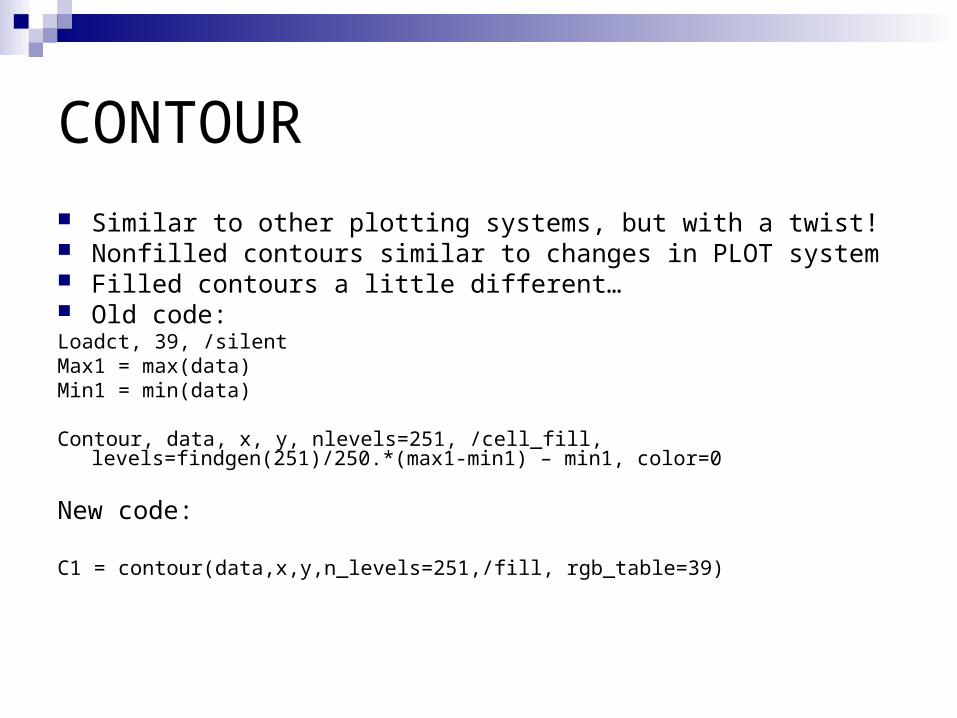
Similar to other plotting systems, but with a twist! Nonfilled contours similar to changes in PLOT system Filled contours a little different… Old code: Loadct, 39, /silentMax1 = max(data)Min1 = min(data)

Contour, data, x, y, nlevels=251, /cell_fill, levels=findgen(251)/250.*(max1-min1) – min1, color=0

New code:

C1 = contour(data,x,y,n_levels=251,/fill, rgb_table=39)

COLORBAR Remember how much of a pain making colorbars was? Not anymore! Old code:

Ncolors=255Loc = [0.1,0.1,0.8,0.125]xsize= (loc(2) – loc(0))*D.X_VSIZEYsize = (loc(3) – loc(1))*D.Y_VSIZEXstart = loc(0)*D.X_VSIZEYstart = loc(3) *D.Y_VSIZE

Bar = BINDGEN(256)#REPLICATE(1B,10)Bar = BYTSCL(bar, top=ncolors-1)

TV, CONGRID(bar, xsize, ysize), xstart+1, ystart=1

PLOT, findgen(251)/250., findgen(251)/250.*max1, /nodata, $ position=loc, yticks=1, ytickformat=‘(A1)’ yminor=1, xticklen=0.25,$ xrange=[min1,max1], xtitle=title1, color=0, /noerase, xstyle=1

New code:

Loc = [0.1,0.1,0.8,0.125]cbar1 = colorbar(target = c1, position = loc)

CONTOUR and COLORBAR

Let’s go to the code… looking at the wind speed example

contour_windspeed.pro

IMAGE

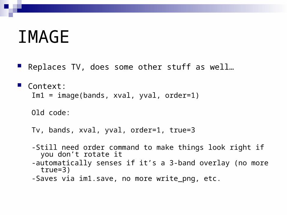
Replaces TV, does some other stuff as well…

Context: Im1 = image(bands, xval, yval, order=1)

Old code:

Tv, bands, xval, yval, order=1, true=3

-Still need order command to make things look right if you don’t rotate it-automatically senses if it’s a 3-band overlay (no more true=3)-Saves via im1.save, no more write_png, etc.

MAP

Most overhauled routine Moves it into more GIS/ENVI type mapping versus IDL

direct mapping Calling context:

M1 = map(‘Equirectangular’, limit = [min(lat), min(lon), max(lat), max(lon)], position=[0.1,0.1,0.9,0.9], dimension=[900,900]

Replaces: Map_set, limit = [min(lat), min(lon), max(lat), max(lon)], position = [0.1,0.1,0.9,0.9]

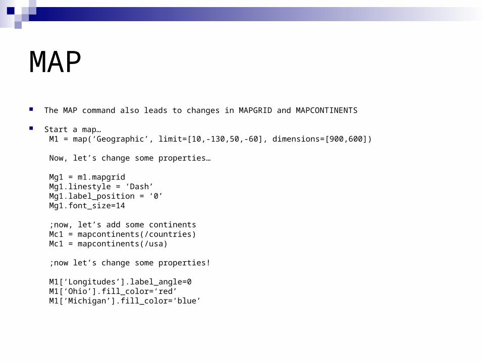
MAP The MAP command also leads to changes in MAPGRID and MAPCONTINENTS

Start a map…M1 = map(‘Geographic’, limit=[10,-130,50,-60], dimensions=[900,600])

Now, let’s change some properties…

Mg1 = m1.mapgridMg1.linestyle = ‘Dash’Mg1.label_position = ‘0’Mg1.font_size=14

;now, let’s add some continentsMc1 = mapcontinents(/countries)Mc1 = mapcontinents(/usa)

;now let’s change some properties!

M1[‘Longitudes’].label_angle=0M1[‘Ohio’].fill_color=‘red’M1[‘Michigan’].fill_color=‘blue’

MAP

The map works in projection space, not in the direct space anymore

So, let’s say we want to plot points in the map… of the NARR grid or something

Let’s go to plot_narr_latlon.pro

VECTOR and STREAMLINE

Two new ways to plot wind features! Some of these are pretty awesome!

Context:V1 = vector(uwind, vwind, x, y,

vector_style=‘barbs’)

St1 = streamline(uwind, vwind, x, y, streamline_stepsize=0.1, streamline_nsteps=200)

Let’s go to the code: start with stream_vector.pro

Combination plots!

OK, so we have covered mapping, plotting, streamlines, vectors, colorbars…

Now let’s put some of these together in IDL 8.0 syntax.

Let’s look at combo_plot.pro and go from there…

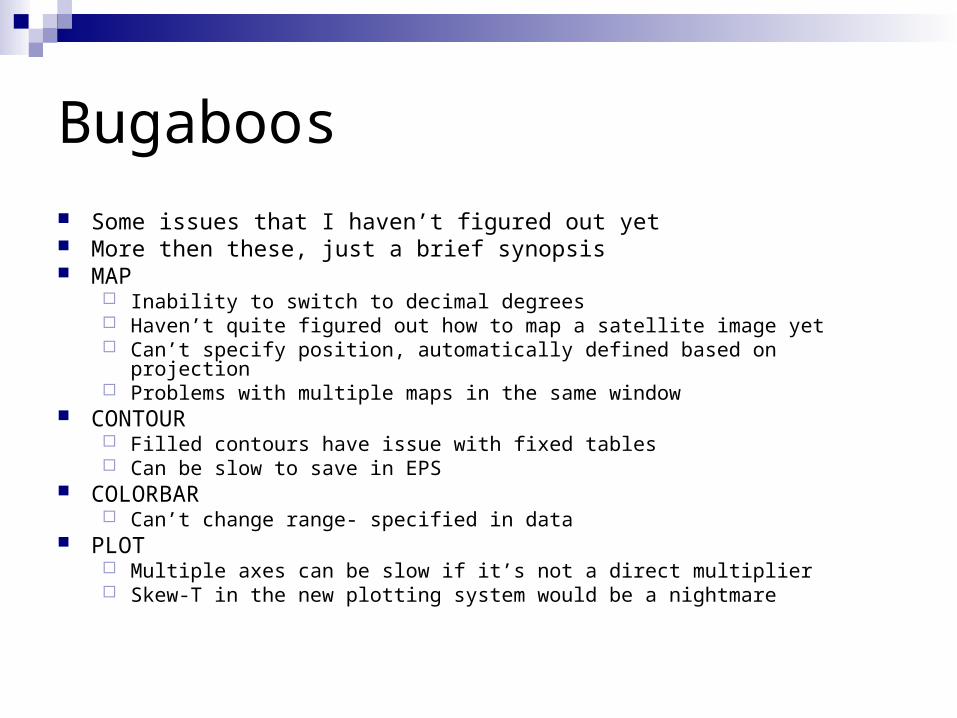
Bugaboos

Some issues that I haven’t figured out yet More then these, just a brief synopsis MAP

Inability to switch to decimal degrees Haven’t quite figured out how to map a satellite image yet Can’t specify position, automatically defined based on projection Problems with multiple maps in the same window

CONTOUR Filled contours have issue with fixed tables Can be slow to save in EPS

COLORBAR Can’t change range- specified in data

PLOT Multiple axes can be slow if it’s not a direct multiplier Skew-T in the new plotting system would be a nightmare

Overview

IDL 8.0 makes simple things easier! IDL 8.0 makes complex things harder!

Overall, adapt code as you see fit- I’m moving most of my new simple plotting (especially error and bar plots) to the new system, but will probably keep the old Direct Graphics for mapping and filled contours