Embed Size (px)
Citation preview

IEEE Copyright Statement: Copyright © [2007] IEEE. Reprinted from Proceedings of the IEEE, Special Issue on Networked Control Systems. Vol. 95, Issue 1, January 2007. This material is posted here with permission of the IEEE. Such permission of the IEEE does not in any way imply IEEE endorsement of any of Carnegie Mellon University's products or services. Internal or personal use of this material is permitted. However, permission to reprint/republish this material for advertising or promotional purposes or for creating new collective works for resale or redistribution must be obtained from the IEEE by writing to [email protected]. By choosing to view this document, you agree to all provisions of the copyright laws protecting it.

INV ITEDP A P E R
Foundations of Control andEstimation Over Lossy NetworksMathematical tools are proposed for optimal design of networked control
systems when physical link losses limit available information.
By Luca Schenato, Member IEEE, Bruno Sinopoli, Member IEEE,
Massimo Franceschetti, Member IEEE, Kameshwar Poolla, and
S. Shankar Sastry, Fellow IEEE
ABSTRACT | This paper considers control and estimation
problems where the sensor signals and the actuator signals are
transmitted to various subsystems over a network. In contrast
to traditional control and estimation problems, here the
observation and control packets may be lost or delayed. The
unreliability of the underlying communication network is
modeled stochastically by assigning probabilities to the
successful transmission of packets. This requires a novel
theory which generalizes classical control/estimation para-
digms. The paper offers the foundations of such a novel theory.
The central contribution is to characterize the impact of the
network reliability on the performance of the feedback loop.
Specifically, it is shown that for network protocols where
successful transmissions of packets is acknowledged at the
receiver (e.g., TCP-like protocols), there exists a critical
threshold of network reliability (i.e., critical probabilities for
the successful delivery of packets), below which the optimal
controller fails to stabilize the system. Further, for these
protocols, the separation principle holds and the optimal LQG
controller is a linear function of the estimated state. In stark
contrast, it is shown that when there is no acknowledgement of
successful delivery of control packets (e.g., UDP-like protocols),
the LQG optimal controller is in general nonlinear. Conse-
quently, the separation principle does not hold in this
circumstance.
KEYWORDS | LQG control; networked control systems; opti-
mal estimation; packet drop; separation principle; stability;
TCP; UDP
I . INTRODUCTION
The rapid convergence of sensing, computing and wireless
communication technologies on cost effective, low power,
miniature devices, is enabling a host of new control
applications. In recent years, we have witnessed wireless
technologies replacing wired counterparts in all applica-
tions where it can be securely and reliably implemented.
Particularly notable is the case of cellular telephony, that is
rapidly driving wireline telephony to obsolescence. Sim-ilarly, LAN access is now dominated by WI-FI. The next
dominos to fall are likely to be wired broadband access
technologies such as DSL, which will be replaced by
WIMax and 3G wireless data services.
In recent years, sensor technology has witnessed
extraordinary growth. Everything is getting Bsensed:[vehicles, roads, buildings, airspaces, and the environment.
Sensors are getting smaller, cheaper, pervasive, and morepowerful. The confluence of sensing technology and wire-
less communication will spawn a plethora of new tech-
nological opportunities. Indeed, the ability to inexpensively
gather data over a network at a very fine temporal and
spatial granularity, and the ability to process this data in
real-time and then perform appropriate control actions, is
enabling the development of a number of new applications
[1]–[3]. The possibilities created by wireless sensor net-works are extraordinary. These include real time alarm
systems for catastrophic, yet predictable events, such as
tsunamis, landslides, and rail accidents. Another potential
Manuscript received August 8, 2005; revised July 28, 2006. This work was supported
in part by DARPA under Grant F33615-01-C-1895, in part by the National Science
Foundation (NSF) under CAREER Award CNS-0546235, in part by the European
Community Research Information Society Technologies under Grant RECSYS
IST-2001-32515, and under Marie Curie International Reintegration Grant
SENSNET-MIRG-6-CT-2005-014815.
L. Schenato is with the Department of Information Engineering, University of Padova,
35100 Padova, Italy (e-mail: [email protected]).
B. Sinopoli, K. Poolla, and S. Sastry are with the Department of Electrical
Engineering, the University of California at Berkeley, Berkeley, CA 94720-1770 USA
(e-mail: [email protected]; [email protected];
M. Franceschetti is with the Department of Electrical and Computer Engineering,
the University of California at San Diego, La Jolla, CA 92093-0407 USA
(e-mail: [email protected]).
Digital Object Identifier: 10.1109/JPROC.2006.887306
Vol. 95, No. 1, January 2007 | Proceedings of the IEEE 1630018-9219/$25.00 �2007 IEEE

application is using sensor networks to efficiently andreliably control electric power grids by exchanging load
information between local stations and optimizing power
delivery while avoiding costly and dangerous blackouts.
Realizing the promise of sensor network technologies
requires the development of theoretical foundations of
remote control over unreliable networks. This will enable
the evolution of design rules, the navigation of perfor-
mance-complexity tradeoffs, and the systematic design ofsensor networks for various target applications.
The benefits of pervasive networking and sensing are
compelling. For example buildings, both residential and
commercial, can greatly benefit from the use of sensor
networks, by decreasing construction and operating costs,
while improving comfort and safety. Today, installation
(and particularly wiring) accounts for more than half of the
cost of an Heating, Ventilation, Air Conditioning (HVAC)system in a building. Wireless communication could
sensibly lower this cost [4], [5]. Moreover, combining
wireless technology with Micro Electro Mechanical
Systems (MEMS) technology could further lower cost,
allowing sensors to be embedded in products such as
ceiling tiles and furniture, and enable improved control of
the indoor environment [6]. These sensor networks could
dramatically improve energy efficiency in buildings.Another example where sensor networks technology is
anticipated to have a significant impact is Supervisory
Control And Data Acquisition (SCADA) networks [7], [8].
These networks, were originally developed in the 1960s,
and are used for industrial measurement, monitoring, and
control systems, especially by electricity and natural gas
utilities, water and sewage utilities, railroads, telecommu-
nications, and other critical infrastructure components.They enable remote monitoring and control of a large
variety of industrial devices, such as water and gas pumps,
track switches, and traffic signals.
SCADA systems typically implement a distributed
system whose elements are called points. A point can be a
single input or output value, monitored or controlled by the
system. A variety of host computers allow for Bsupervisory
level[ control of the remote site. The majority of the controldecisions take place at distributed locations called Remote
Terminal Units (RTUs). RTUs connect to physical equip-
ment such as switches, pumps and other devices, and
monitor and control these devices. SCADA systems often
have Distributed Control System (DCS) components. In
this case smart RTUs are employed, capable of performing
autonomous control and decision without the intervention
of the master computers. The role of host computers isgenerally restricted to supervisory level control. Data
acquisition begins at the RTU level and includes meter
readings and equipment statuses that are communicated to
the SCADA as required. Data is then compiled and
formatted so that a control room operator using the SCADA
system can cogently make appropriate supervisory deci-
sions that may required over-riding normal RTU controls.
SCADA systems have traditionally used combinations ofvarious infrastructure technologies to meet communication
requirements. The existence of a consolidated wired legacy
infrastructure has impeded the development of open sys-
tems based on wireless technology. Wireless technology
could provide superior performance and lower costs, with
simpler maintenance and upgradability. Most of the remote
monitoring and control application could run over the
wireless infrastructure, while components could be easilyswapped without any service interruption.
A third example of application of sensor networks
technology is automotive vehicle networks. Electronics is
quickly becoming a primary differentiator in the automo-
tive industry, with vendors offering electronic services
such as Global Positioning System (GPS), in-vehicle safety
and security system, DVD, and drive-by-wire systems [9].
Electronic systems now account for a sizeable part of thecost and weight of a vehicle. Cars have over 50 embedded
computers running a variety of applications, from safety-
critical to pure entertainment. These applications typically
consist of sensors, actuators, and controllers that are
spatially distributed in the vehicle. These components
communicate using dedicated wires, bringing the length of
wires in high-end luxury cars to amount for more than
three miles and adding over two hundred pounds of weightto the vehicle [10]. As the need for electronics is likely to
in increase with new services and applications, this
wireline design scheme is unsustainable. In-vehicle
networking will become essential and a prime application
of networked embedded systems theory. As many applica-
tions converge in sharing computing and communication
resources, issues of scheduling, network delay and data
loss will need to be dealt with systematically.In examining the applications detailed above, a
common pattern emerges. Data is sent from possibly
multiple sensors to one or more computing units, using a
communication network. Such data are then processed to
estimate the state of a dynamical system, and actuator
signals are sent to actuators using the same network. Both
measurements and actuator signals have very stringent
timing constraints that the network needs to be able tomeet. The presence of a communication network in the
feedback control loop raises a number of issues. One of
the key parameters in digital control systems design is the
selection of a fixed sampling period. This is mainly a
function of the system dynamics, and it places a hard
constraint on the time necessary to receive observations,
estimate the state, compute the subsequent control inputs,
and transmit these to the actuators. All of this needs tohappen within a single sampling interval. The computing
power of modern processors combined with wired,
dedicated interconnections between various subsystems
usually guarantees that such constraints are met. In
designing feedback control systems around wireless sensor
networks, the implicit assumption of data availability no
longer holds, as data packets are randomly dropped and
Schenato et al.: Foundations of Control and Estimation Over Lossy Networks
164 Proceedings of the IEEE | Vol. 95, No. 1, January 2007

delayed. While classical control theories provide a wealthof analytical results, they critically rely on the assumption
that the underlying communication technology is ideal. In
the wireless communication setting, neglecting nonideal-
ities such as packet loss can result in catastrophic closed-
loop performance.
This paper attempts to lay the theoretical foundations
for estimation and control system design problems while
explicitly accounting for realities of the underlyingwireless communication network.
II . CONTROL OVER NETWORKS
A. FoundationsWireless networks are inherently less reliable and
secure than their wired counterparts. These two factors
limit the penetration of wireless technology in many
application contexts. For example, car manufacturers are
reluctant to deploy wireless networks in cars, especially forconnecting safety-critical systems such as braking and
steering. Loss of data may have a disastrous effect on the
behavior of the vehicle. Similarly, in SCADA systems,
which represent the standard control infrastructure in
industrial processes and also in some experimental
facilities such as nuclear fusion, communication is
ethernet based, and it is likely to remain so until we can
guarantee acceptable performance and security. In short,applications need to be designed robust to unreliability in
the network.
Issues of communication delay, data loss, and time-
synchronization play critical roles. In particular, commu-
nication and control are tightly coupled and they cannot be
addressed independently. Specific questions that arise are
the following. What is the amount of data loss that the
control loop can tolerate while reliably performing itstask? Can communication protocols be designed to satisfy
this constraint? The goal of this paper is to provide some
first steps in answering such questions by examining the
basic system-theoretic implications of using unreliable
networks for control. This requires a generalization of
classical control techniques that explicitly takes into
account the stochastic nature of the communication
channel.We begin by addressing some simple canonical
problems that will shed some light on the real system
behavior. We shall consider the following abstractions.
Packet networks communication channels typically use
one of two fundamentally different protocols: TCP-like or
UDP-like. In the first case there is acknowledgement of
received packets, while in the second case no-feedback is
provided on the communication link. The well knownTransmission Control (TCP) and User Datagram (UDP)
protocols used in the Internet are specific examples of our
more general notion of TCP-like and UDP-like communi-
cation protocol classes. We want to study the effect of data
losses due to the unreliability of the network links underthese two general protocol abstractions. Accordingly, we
model the arrival of both observations and control packets
as random processes whose parameters are related to the
characteristics of the communication channel. Two in-
dependent Bernoulli processes are considered, with
parameters � and �, that govern packet losses between
the sensors and the estimation-control unit, and between
the latter and the actuation points, see Fig. 1. We remarkthat using Bernoulli processes is clearly an idealization
that is chosen for mathematical tractability. The network-
ing component obviously has an additional impact on the
performance of the closed loop systems. Routing and
congestion control mechanisms would affect the packet
arrival probability and it is necessary in practice to
estimate this probability to compute the optimal control
law. The presence of correlations in the packet loss processcan be taken into account, in principle, at the cost of
complicating the mathematical analysis. Our foundations
are instead based on simple abstractions which, as we shall
see, reveal useful design guidelines and can explain real
system behaviors that are observed in practice.
B. Previous WorkStudy of stability of dynamical systems where compo-
nents are connected asynchronously via communication
channels has received considerable attention in the past
few years and our contribution can be put in the context of
the previous literature. In [11] and [12], the authors
proposed to place an estimator, i.e., a Kalman filter, at the
sensor side of the link without assuming any statistical
model for the data loss process. In [13], Smith et al.considered a suboptimal but computationally efficientestimator that can be applied when the arrival process is
modeled as a Markov chain, which is more general than a
Bernoulli process. Other works include Nilsson et al. [14],
[15] who present the LQG optimal regulator with bounded
delays between sensors and controller, and between the
controller and the actuator. In this work, bounds for the
critical probability values are not provided and there is no
analytic solution for the optimal controller. The casewhere dropped measurements are replaced by zeros is
considered by Hadjicostis and Touri [16], but only in the
scalar case. Other approaches include using the last
received sample for control [15], or designing a dropout
compensator [17], which combines estimation and control
in a single process. However, the former approach does
not consider optimal control and the latter is limited to
scalar systems. Yu et al. [18] studied the design of anoptimal controller with a single control channel and
deterministic dropout rates. Seiler et al. [19] considered
Bernoulli packet losses only between the plant and the
controller and posed the controller design as an H1optimization problem. Other authors [20]–[23] model
networked control systems with missing packets as
Markovian jump linear systems (MJLSs), however this
Schenato et al. : Foundations of Control and Estimation Over Lossy Networks
Vol. 95, No. 1, January 2007 | Proceedings of the IEEE 165

approach gives suboptimal controllers since the estimators
are stationary. Finally, Elia [24], [25] proposed to model
the plant and the controller as deterministic time invariantdiscrete-time systems connected to zero-mean stochastic
structured uncertainty. The variance of the stochastic
perturbation is a function of the Bernoulli parameters, and
the controller design is posed an an optimization problem
to maximize mean-square stability of the closed loop
system. This approach allows analysis of Multiple Input
Multiple Output (MIMO) systems with many different
controller and receiver compensation schemes [24],
however, it does not include process and observation
noise and the controller is restricted to be time-invariant,
hence suboptimal. There is also an extensive literature,inspired by Shannon’s results on the maximum bit-rate
that a channel with noise can reliably carry, whose goal is
to determine the minimum bit-rate that is needed to
stabilize a system through feedback [26]–[35]. This
approach is somewhat different from ours as we consider
bits to be grouped into packets that form single entities
which can be lost. Nonetheless there are several similar-
ities that are not yet fully explored.
Fig. 1. Architecture of the closed loop system over a communication network under TCP-like protocols (top) and UDP-like protocols (bottom).
The binary random variables �t and �t indicates whether packets are transmitted successfully.
Schenato et al.: Foundations of Control and Estimation Over Lossy Networks
166 Proceedings of the IEEE | Vol. 95, No. 1, January 2007

Compared to previous works, this paper considers thealternative approach where the external compensator
feeding the controller is the optimal time varying Kalman
gain. Moreover, this paper considers the general Multiple
Input Multiple Output (MIMO) case, and gives some
necessary and sufficient conditions for closed loop
stability. The work of [36] is most closely related to this
paper. However, we consider the more general case when
the matrix C is not the identity and there is noise in theobservation and in the process. In addition, we also give
stronger necessary and sufficient conditions for existence
of the solution in the infinite horizon LQG control.
C. Our ContributionWe study the effect of data losses due to the unreli-
ability of the network links under two different classes of
protocols. In our analysis, the distinction between the twoclasses of protocols will reside exclusively in the availability
of packet acknowledgement. Adopting the framework
proposed by Imer et al. [36], we will refer, therefore, to
TCP-like protocols if packet acknowledgement is available
and to UDP-like protocols otherwise.
We show that, for the TCP-like case, the classic
separation principle holds, and consequently the control-
ler and estimator can be designed independently. More-over, the optimal controller is a linear function of the state.
In sharp contrast, for the UDP-like case, a counter-
example demonstrates that the optimal controller is in
general nonlinear. In the special case when the state is
fully observable and the observation noise is zero, the
optimal controller is indeed linear. We explicitly note that
a similar, but slightly less general special case was
previously analyzed in [36], where both observation andprocess noise are assumed to be zero and the input
coefficient matrix to be invertible.
Our final set of results relate to convergence in the
infinite horizon. Here, results on estimation with missing
observation packets [37], [38] are extended to the control
case. We show the existence of a critical domain of values
for the parameters of the Bernoulli arrival processes, � and
�, outside which a transition to instability occurs and theoptimal controller fails to stabilize the system.
These results are visually summarized in Fig. 2, where
our stability bounds are depicted for a scalar system. The
stability regions are the regions above those bounds. No-
tice that for TCP-like protocols there exist critical arrival
probabilities for the control and observation packets below
which the system is in the unstable region. These critical
values are independent of each other, which is anotherconsequence of the fact that the separation principle holds
for these protocols.
In contrast, for UDP-like protocols the critical arrival
probabilities for the control and observation channels are
coupled, and the stability domain boundary assumes a
curved form. The performance of the optimal controller
degrades considerably when compared to TCP-like proto-
cols, as the stability region of UDP is strictly contained into
the one of TCP. Finally, the figure also reports the
boundary of a weaker condition on the stability region for
UDP-like protocols as reported in [36], which is indicated
with a dashed line.
III . PROBLEM FORMULATION
Consider the following linear stochastic system with
intermittent observation and control packets:
xkþ1 ¼ Axk þ Buak þ wk (1)
uak ¼ �kuc
k (2)
yk ¼ �kCxk þ vk (3)
where uak is the control input to the actuator, uc
k is the
desired control input computed by the controller,
ðx0;wk; vkÞ are Gaussian, uncorrelated, white, with mean
ð�x0; 0; 0Þ and covariance ðP0;Q; RÞ respectively, and
ð�k; �kÞ are i.i.d. Bernoulli random variables withPð�k ¼ 1Þ ¼ �� and Pð�k ¼ 1Þ ¼ ��. The stochastic variable
�k models the packet loss between the controller and the
actuator: if the packet is correctly delivered then uak ¼ uc
k,
otherwise if it is lost then the actuator does nothing, i.e.,
uak ¼ 0. This compensation scheme is summarized by (2).
This modeling choice is not unique: for example if the
control packet uck is lost, the actuator could employ the
previous control value, i.e., uak ¼ ua
k�1, as suggested in [15].The analysis of this scheme requires a different problem
Fig. 2. Stability regions for TCP-like protocols and UDP-like protocols
for a scalar unstable system. These bounds are tight (i.e., necessary
and sufficient) in the scalar case. The dashed line corresponds
to the boundary of a weaker (sufficient) condition on the stability
region for UDP-like protocols as recently reported in [36].
Schenato et al. : Foundations of Control and Estimation Over Lossy Networks
Vol. 95, No. 1, January 2007 | Proceedings of the IEEE 167

formulation and is not considered here. However, bothschemes are natural compensation methods for input
packet loss, and in Section VII an empirical comparison
seems to suggest that the zero-input scheme indeed
outperforms the hold-input scheme. The stochastic vari-
able �k models the packet loss between the sensor and the
controller: if the packet is delivered then yk ¼ Cxk þ vk,
while if the packet is lost the controller reads pure noise,
i.e., yk ¼ vk. This observation model is summarized by (3).A different observation formalism was proposed in [37],
where the missing observation was modeled as an obs-
ervation for which the measurement noise had infinite
covariance. It is possible to show that both models are
equivalent, but the one considered in this paper has the
advantage of simplifying the equations. This is because at
times when packets are not delivered, the optimal
estimator ignores the observation yk, therefore, its valueis irrelevant.
Let us define the following information sets:
I k ¼ F k ¼� fyk;Gk;Nk�1g; TCP-like
Gk ¼� fyk;Gkg; UDP-like
((4)
where yk ¼ ðyk; yk�1; . . . ; y1Þ, Gk ¼ ð�k; �k�1; . . . ; �1Þ, and
Nk ¼ ð�k; �k�1; . . . ; �1Þ.Consider also the following cost function:
JNðuN�1; �x0; P0Þ ¼ E x0NWNxN
�þXN�1
k¼0
x0kWkxk þ �ku0kUkuk
� �juN�1; �x0; P0
#(5)
where uN�1 ¼ ðuN�1; uN�2; . . . ; u1Þ. Note that we are
weighting the input only if it is successfully received at
the plant. In the event it is not received, the plant applies
zero input and, therefore, there is no energy expenditure.
We now seek a control input sequence u�N�1 as a
function of the admissible information set I k, i.e.,
uk ¼ gkðI kÞ, that minimizes the functional defined in(5), i.e.,
J�Nð�x0; P0Þ ¼� minuk¼gkðI kÞ
JNðuN�1; �x0; P0Þ (6)
where I k ¼ fF k;Gkg is one of the sets defined in (4). The
set F corresponds to the information provided under an
acknowledgement-based communication protocols (TCP-
like) in which successful or unsuccessful packet delivery at
the receiver is acknowledged to the sender within the samesampling time period. The set G corresponds to the
information available at the controller under communica-
tion protocols in which the sender receives no feedback
about the delivery of the transmitted packet to the receiver
(UDP-like). The UDP-like schemes are simpler to imple-
ment than the TCP-like schemes from a communication
standpoint. Moreover UDP-like protocols includes broad-
casting which is not feasible under TCP-like protocols.However, UDP-like protocols provide a leaner information
set. The goal of this paper is to design optimal LQG
controllers and to estimate their closed-loop performance
for both TCP-like and UDP-like protocols.
IV. OPTIMAL ESTIMATION
We start defining the following variables:
x̂kjk ¼�E½xkjI k�
ekjk ¼�
xk � x̂kjk
Pkjk ¼�E ekjke0kjkjI k
h i: (7)
Derivations below will make use of the following facts:
Lemma 4.1: The following facts are true [39]:
(a) E½ðxk�x̂kÞx̂0kjI k� ¼ E½ekjkx̂0kjI k� ¼ 0;
(b) E½x0kSxkjI k� ¼x̂0kSx̂k þ traceðSPkjkÞ, 8S � 0;(c) E½E½gðxkþ1ÞjI kþ1�jI k� ¼ E½gðxkþ1ÞjI k�, 8gð�Þ.We now make the following computations which we
use to derive the optimal LQG controller
E x0kþ1Sxkþ1jI k
� ¼ E x0kA0SAxkjI k
� þ ��u0kB0SBuk þ 2��u0kB0SAx̂kjk þ traceðSQÞ (8)
where both the independence of �k, wk, xk, and the zero-
mean property of wk are exploited. The previous expecta-
tion holds true for both the information sets, i.e., I k ¼ F k
or I k ¼ Gk. Also
E e0kjkTekjkjI k
h i¼ trace TE ekjke0kjkjI k
h i �¼ traceðTPkjkÞ; 8T � 0:
The equations for the optimal estimator are different
whether TCP-like or UDP-like communication protocols
are used.
Schenato et al.: Foundations of Control and Estimation Over Lossy Networks
168 Proceedings of the IEEE | Vol. 95, No. 1, January 2007

A. Estimator Design Under TCP-Like ProtocolsEquations for optimal estimator are derived using
arguments similar to those used in standard Kalman
filtering. The innovation step is given by
x̂kþ1jk ¼�
AE½xkjF k� þ �kBuk ¼ Ax̂kjk þ �kBuk (9)
ekþ1jk ¼�
xkþ1 � x̂kþ1jk ¼ Aekjk þ wk (10)
Pkþ1jk ¼�E ekþ1jke0kþ1jkj�k;F k
h i¼ APkjkA0 þ Q (11)
where the independence of wk and F k, and the require-
ment that uk is a deterministic function of F k, are used.Since ykþ1, �kþ1, wk and F k are independent, the
correction step is given by
x̂kþ1jkþ1¼ x̂kþ1jkþ�kþ1Kkþ1ðykþ1�Cx̂kþ1jkÞ (12)
ekþ1jkþ1¼�
xkþ1�x̂kþ1jkþ1
¼ ðI��kþ1Kkþ1CÞekþ1jk��kþ1Kkþ1vkþ1 (13)
Pkþ1jkþ1¼ Pkþ1jk��kþ1Kkþ1CPkþ1jk (14)
Kkþ1¼�
Pkþ1jkC0ðCPkþ1jkC0 þ RÞ�1 (15)
where we simply applied the standard derivation for the
time varying Kalman filter using the following time varying
system matrices: Ak ¼ A, Ck ¼ �kC, and CovðvkÞ ¼ R.
B. Estimator Design Under UDP-Like ProtocolsWe derive the equations for the optimal estimator
using similar arguments as in the standard Kalman
filtering equations. The innovation step is given by
x̂kþ1jk ¼�E½xkþ1jGk� ¼ E½Axk þ �kBuk þ wkjGk�
¼ Ax̂kjk þ ��Buk (16)
ekþ1jk ¼�
xkþ1 � x̂kþ1jk
¼ Aekjk þ ð�k � �ÞBuk þ wk (17)
Pkþ1jk ¼�E ekþ1jke0kþ1jkjGk
h i¼ APkjkA0 þ ��ð1 � ��ÞBuku0kB0 þ Q (18)
where we used the independence and zero-mean of wk,
ð�k � ��Þ, and Gk, and the fact that uk is a deterministic
function of the information set Gk. Note how under UDP-
like communication, differently from TCP-like, the error
covariance Pkþ1jk depends explicitly on the control input
uk. This is the main difference with control feedback
systems under TCP-like protocols.
The correction step is the same as for the TCP case
x̂kþ1jkþ1 ¼ x̂kþ1jk þ �kþ1Kkþ1ðykþ1 � Cx̂kþ1jkÞPkþ1jkþ1 ¼ Pkþ1jk � �kþ1Kkþ1CPkþ1jk; (19)
Kkþ1 ¼� Pkþ1jkC0ðCPkþ1jkC0 þ RÞ�1(20)
where again we considered a time varying system with
Ak ¼ A and Ck ¼ �kC as we did for the optimal estimator
under TCP-like protocols.
V. OPTIMAL CONTROL UNDERTCP-LIKE PROTOCOLS
Derivation of the optimal feedback control law and the
corresponding value for the objective function will follow
the dynamic programming approach based on the cost-to-
go iterative procedure.Define the optimal value function VkðxkÞ as follows:
VNðxNÞ ¼�E x0NWNxNjFN
� VkðxkÞ ¼
�min
uk
E x0kWkxk þ �ku0kUkuk
�þ Vkþ1ðxkþ1ÞjF k� (21)
where k ¼ N � 1; . . . ; 1. Using dynamic programming
theory [40], one can show that J�N ¼ V0ðx0Þ. Under TCP-
like protocols the following lemma holds true:
Lemma 5.1: The value function VkðxkÞ defined in (21) for
the system dynamics of (1)–(3) under TCP-like protocolscan be written as
VkðxkÞ ¼ E x0kSkxkjF k
� þ ck; k ¼ N; . . . ; 0 (22)
where the matrix Sk and the scalar ck can be computed
recursively as follows:
Sk ¼ A0Skþ1A þ Wk
� ��A0Skþ1BðB0Skþ1B þ UkÞ�1B0Skþ1A (23)
ck ¼ trace ðA0Skþ1A þ Wk � SkÞPkjk� �
þ traceðSkþ1QÞ þ E½ckþ1jF k� (24)
with initial values SN ¼ WN and cN ¼ 0. Moreover the
optimal control input is given by
uk ¼ �ðB0Skþ1B þ UkÞ�1B0Skþ1Ax̂kjk ¼ Lkx̂kjk: (25)
Proof: The proof employs an induction argument. The
claim is clearly true for k ¼ N with the choice of parameters
Schenato et al. : Foundations of Control and Estimation Over Lossy Networks
Vol. 95, No. 1, January 2007 | Proceedings of the IEEE 169

SN ¼WN and cN ¼ 0. Suppose now that the claim is true fork þ 1, i.e., Vkþ1ðxkþ1Þ ¼ E½x0kþ1Skþ1xkþ1jF kþ1� þ ckþ1. The
value function at time step k is the following:
VkðxkÞ ¼ minuk
E x0kWkxk þ �ku0kUkuk þ Vkþ1ðxkþ1ÞjF k
� ¼ min
uk
E x0kWkxk þ �ku0kUkuk þ jF k
� þ E E x0kþ1Skþ1xkþ1 þ ckþ1jF kþ1
� jF k
� ¼ min
uk
E x0kWkxk þ �ku0kUkuk
�þ x0kþ1Skþ1xkþ1 þ ckþ1jF k
¼ E x0kWkxk þ x0kA0Skþ1AxkjF k
� þ traceðSkþ1QÞ þ E½ckþ1jF k�þ ��min
uk
u0kðUk þ B0Skþ1BÞuk
�þ 2u0kB0Skþ1Ax̂kjk
�(26)
where we used Lemma 1(c) to get the third equality, and (8)to obtain the last equality. The value function is a quadratic
function of the input, therefore, the minimizer can be
simply obtained by solving @Vk=@uk ¼ 0, which gives (25).
The optimal feedback is, thus, a simple linear function of the
estimated state. If we substitute the minimizer back into
(26) we get
VkðxkÞ ¼ E x0kWkxk þ x0kA0Skþ1AxkjI k
� þ traceðSkþ1QÞ þ E½ckþ1jI k�� ��x̂0kjkA0Skþ1BðUk þ B0Skþ1BÞ�1B0Skþ1Ax̂kjk
¼ E x0kWkxk þ x0kA0Skþ1Axk � ��x0kA0Skþ1B��ðUk þ B0Skþ1BÞ�1B0Skþ1AxkjI k
þ traceðSkþ1QÞ þ E½ckþ1jI k�þ ��trace A0Skþ1BðUk þ B0Skþ1BÞ�1B0Skþ1Pkjk
� �where we used Lemma 1(b). Therefore, the claim given by
(22) is satisfied also for time step k for all xk if and only if the
(23) and (24) are satisfied. hSince J�Nð�x0; P0Þ ¼ V0ðx0Þ, from the lemma it follows
that the cost function for the optimal LQG using TCP-like
protocols is given by
J�N ¼ �x00S0�x0 þ traceðS0P0Þ þXN�1
k¼0
traceðSkþ1QÞ
þXN�1
k¼0
trace ðA0Skþ1A þ Wk � SkÞE� ½Pkjk�� �
(27)
where we used the fact E½x�0S0x0� ¼�x�0S0�x0 þ traceðS0P0Þ,and E� ½�� explicitly indicates that the expectation is
calculated with respect to the arrival sequence f�kg.
It is important to remark that the error covariancematrices fPkjkgN
k¼0 are stochastic since they depend on the
sequence f�kg. Moreover, since the matrix Pkþ1jkþ1 is a
nonlinear function of the previous time step matrix cov-
ariance Pkjk, as can be observed from (11) and (15), the exact
expected value of these matrices, E�½Pkjk�, cannot be
computed analytically, as shown in [37]. However, they
can be bounded by computable deterministic quantities, as
shown in [37] from which we can derive the followinglemma:
Lemma 5.2 ([37]): The expected error covariance matrix
E� ½Pkjk� satisfies the following bounds:
ePkjk � E� ½Pkjk� � bPkjk 8k � 0 (28)
where the matrices bPkjk and ePkjk can be computed as
follows:
bPkþ1jk ¼ AbPkjk�1A0 þ Q � ��AbPkjk�1C0
� ðCbPkjk�1C0 þ RÞ�1CbPkjk�1A0 (29)bPkjk ¼ bPkjk�1 � ��bPkjk�1C0
� ðCbPkjk�1C0 þ RÞ�1CbPkjk�1 (30)ePkþ1jk ¼ð1 � ��ÞAePkjk�1A0 þ Q (31)ePkjk ¼ð1 � ��ÞePkjk�1 (32)
where the initial conditions are bP0j0 ¼ eP0j0 ¼ P0.
Proof: The argument is based on the observation that
the matrices Pkþ1jk and Pkjk are concave and monotonic
functions of Pkjk�1. The proof is offered in [37] and is thus
omitted. hFrom this lemma it follows that also the minimum
achievable cost J�N, given by (27), cannot be computed
analytically, but can bounded as follows:
JminN � J�N � Jmax
N (33)
JmaxN ¼ �x00S0�x0 þ traceðS0P0Þ þ
XN�1
k¼0
traceðSkþ1QÞÞ
þXN�1
k¼0
trace ðA0Skþ1A þ Wk � SkÞbPkjk� �
(34)
JminN ¼ �x00S0�x0 þ traceðS0P0Þ þ
XN�1
k¼0
traceðSkþ1QÞ
þXN�1
k¼0
trace ðA0Skþ1A þ Wk � SkÞePkjk� �
: (35)
Schenato et al.: Foundations of Control and Estimation Over Lossy Networks
170 Proceedings of the IEEE | Vol. 95, No. 1, January 2007

The results derived above can be summarized asfollows:
Theorem 5.3: Consider the system (1)–(3) and consider
the problem of minimizing the cost function (5) within the
class of admissible policies uk ¼ fðF kÞ, where F k is the
information available under TCP-like schemes, given in
(4). Then, the following hold.
a) The separation principle still holds for TCP-likecommunication, since the optimal estimator,
given by (9), (11), (12), (14), and (15), is inde-
pendent of the control input uk.
b) The optimal estimator gain Kk is time-varying
and stochastic since it depends on the past ob-
servation arrival sequence f�jgkj¼1.
c) The optimal control input, given by (25) and (23)
with initial condition SN ¼ WN, is a linearfunction of the estimated state x̂kjk, i.e.,
uk ¼ Lkx̂kjk, and the optimal gain Lk is indepen-
dent of the process sequences f�k; �kg.
The infinite horizon LQG can be obtained by taking
the limit for N ! þ1 of the previous equations.
However, as explained above, the matrices fPkjkgdepend nonlinearly on the specific realization of the
observation sequence f�kg, therefore, the expected errorcovariance matrices E�½Pkjk� and the minimal cost J�Ncannot be computed analytically and do not seem to
have limit [37]. Differently from standard LQG optimal
regulator [41], the estimator gain does not converge to a
steady state value, but is strongly time-varying due to its
dependence on the arrival process f�kg. Moreover,
while the standard LQG optimal regulator always
stabilizes the original system, in the case of observationand control packet losses, the stability can be lost if the
arrival probabilities ��, �� are below a certain threshold.
This observation comes from the study of existence of
solution for a Modified Riccati Algebraic Equation
(MARE), S ¼ �ðS; A; B;W;U; �Þ, which was introduced
by [42] and studied in [25], [37] and [43], where the
nonlinear operator �ð�Þ is defined as follows:
�ðS; A; B;Q; R; �Þ ¼� A0SA þ W � �A0SBðB0SB þ UÞ�1B0SA:
(36)
In particular, (23), i.e., Skþ1 ¼ �ðSk; A; B;W;U; �Þ, is the
dual of the estimator equation presented in [37],
i.e., Pkþ1 ¼ �ðPk; A0; C0;Q; R; �Þ. The results about
the MARE are summarized in the following lemma
Lemma 5.4: Consider the modified Riccati
equation defined in (36). Let A be unstable,
ðA; BÞ be controllable, and ðA;W1=2Þ be observ-able. Then, the following hold.
a) The MARE has a unique strictly positive definitesolution S1 if and only if � 9 �c, where �c is the
critical arrival probability defined as
�c ¼�
inf�
0 � � � 1jS ¼ �ðS; A; B;W;U; �Þ; S � 0f g:
b) The critical probability �c satisfy the following
analytical bounds:
pmin � �c � pmax
pmin ¼� 1 � 1
maxi �ui ðAÞj j2
pmax ¼�
1 � 1Qi �
ui ðAÞj j2
where �ui ðAÞ are the unstable eigenvalues of A.
Moreover, �c ¼ pmin when B is square and
invertible, and �c ¼ pmax when B is rank one.
c) The critical probability can be numerically com-
puted via the solution of the following quasi-
convex LMIs optimization problem
�c ¼ argmin�� ��ðY; ZÞ 9 0; 0 � Y � I:
��ðY; ZÞ ¼Y Y
ffiffiffi�
pZU
12ffiffiffi�
pðYA0 þ ZB0Þ
ffiffiffiffiffiffiffiffiffiffiffi1 � �
pYA0
Y W�1 0 0 0ffiffiffi�
pU
12Z0 0 I 0 0ffiffiffi
�p
ðAY þ BZ0Þ 0 0 Y 0ffiffiffiffiffiffiffiffiffiffiffi1 � �
pAY 0 0 0 Y
26666664
37777775:
d) If � 9 �c, then limk!þ1 Sk ¼ S1 for all initial co-
ditions S0 � 0, where Skþ1 ¼ �ðSk; A; B; W;U; �Þ.The proof of facts a), c), and d) can be found in [37]. The
proof �c ¼ pmin when B is square and invertible can befound in [42], and the proof �c ¼ pmax when B is rank one
in [25].
Differently from standard LQGoptimal regulator, the estimatorgain does not converge to asteady state value.
Schenato et al. : Foundations of Control and Estimation Over Lossy Networks
Vol. 95, No. 1, January 2007 | Proceedings of the IEEE 171

In [37], statistical analysis of the optimal estimator wasgiven, which we report here for convenience:
Theorem 5.5 ([37]): Consider the system (1)–(3) and the
optimal estimator under TCP-like protocols, given by (9),
(11), (12), (14), and (15). Assume that ðA;Q1=2Þ is
controllable, ðA; CÞ is observable, and A is unstable. Then
there exists a critical observation arrival probability �c,
such that the expectation of estimator error covariance isbounded if and only if the observation arrival probability is
greater than the critical arrival probability, i.e.,
E� ½Pkjk� � M 8k iff �� > �c
where M is a positive definite matrix possibly dependent
on P0. Moreover, it is possible to compute a lower and an
upper bound for the critical observation arrival probability
�c, i.e., pmin � �c � �max � pmax, where
�max ¼� inf�
0 � � � 1; jP ¼ �ðP; A0; C0;Q; R; �Þ; P � 0Þf g
where pmin and pmax are defined in Lemma 5.4.
The proof of the previous theorem can be found in [37].
Using the previous theorem and the results from the
previous section, we can prove the following theoremfor the infinite horizon optimal LQG under TCP-like
protocols:
Theorem 5.6: Consider the same system as defined in the
previous theorem with the following additional hypothe-
sis: WN ¼ Wk ¼ W and Uk ¼ U. Moreover, let ðA; BÞ and
ðA;Q1=2Þ be controllable, and let ðA; CÞ and ðA;W1=2Þ be
observable. Moreover, suppose that �� 9 �c and �� 9 �max,where �c and �max are defined in Lemma 5.4 and in
Theorem 5.5, respectively. Then we have the following.
a) The infinite horizon optimal controller gain is
constant
limk!1
Lk ¼ L1 ¼ �ðB0S1B þ UÞ�1B0S1A: (37)
b) The infinite horizon optimal estimator gain Kk,
given by (15), is stochastic and time-varying since
it depends on the past observation arrivalsequence f�jgk
j¼1.
c) The expected minimum cost can be bounded by
two deterministic sequences
1
NJmin
N � 1
NJ�N � 1
NJmax
N (38)
where JminN , Jmax
N converge to the following values:
Jmax1 ¼� lim
N!þ1
1
NJmax
N
¼ trace�ðA0S1A þ W � S1Þ:� bP1 � ��bP1C0ðCbP1C0 þ RÞ�1CbP1� ��
þ traceðS1QÞ
Jmin1 ¼� lim
N!þ1
1
NJmin
N
¼ð1 � ��Þtrace ðA0S1A þ W � S1ÞeP1� �þ traceðS1QÞ
and the matrices S1, P1, P1 are the positive
definite solutions of the following equations:
S1 ¼ A0S1A þ W � ��A0S1BðB0S1B þ UÞ�1B0S1A
P1 ¼ AP1A0 þ Q � ��AP1C0ðCP1C0 þ RÞ�1CP1A0
P1 ¼ ð1 � ��ÞAP1A0 þ Q
:
Proof:a) Since by hypothesis �� 9 �c, from Lemma 5.4(d)
follows that limk!þ1 Sk ¼ S1. Therefore, (37)
follows from (25).
b) This follows from the dependence on the arrival
sequence f�kg of the optimal state estimator given
by (9), (11), (12), (14), and (15).
c) Equation (29) can be written in terms of the
MARE as bPkþ1jk ¼ �ðbPkjk�1; A0; C0;Q; R; �Þ, there-
fore, since �� 9 �max from Lemma 5.4(d) it followsthat limk!þ1 bPkjk�1 ¼ P1, where P1 is the solu-
tion of the MARE P1 ¼ �ðP1; A0; C0;Q; R; �Þ.Also limk!þ1 ePkjk�1 ¼ P1, where ePkjk�1 is defined
in (31) and P1 is the solution of the Lyapunov
equation bP1 ¼ ~AbP1~A0 þ Q, where ~A ¼ ffiffiffiffiffiffiffiffiffiffiffi
1 � ��p
A.
Such solution clearly exists sinceffiffiffiffiffiffiffiffiffiffiffi1 � ��
pG
ð1=pminÞ ¼ 1=maxi j�ui ðAÞj and thus the matrix ~A
is strictly stable. From (30) and (32) it followsthat limk!þ1 bPkjk ¼ P1 � ��P1C0ðCP1C0 þ RÞ�1
CP1 and limk!þ1 ePkjk ¼ ð1 � ��ÞP1. Also
limk!þ1 Skþ1 ¼ limk!þ1 Sk ¼ S1. Finally from
(33)–(35) and the previous observations follow
the claim. h
VI. OPTIMAL CONTROL UNDERUDP-LIKE PROTOCOLS
In this section, we show that the optimal LQG controller,
under UDP-like communication protocols, is in general nota linear function of the state estimate. Consequently,
Schenato et al.: Foundations of Control and Estimation Over Lossy Networks
172 Proceedings of the IEEE | Vol. 95, No. 1, January 2007

estimation and controller design cannot be treated in-
dependently. For this, we construct a counter-example
considering a simple scalar system and we proceed using
the dynamic programming approach. Consider the scalar
system where A ¼ 1, B ¼ 1, C ¼ 1, WN ¼ Wk ¼ 1, Uk ¼ 0,
R ¼ 1, Q ¼ 0. Analogously to the TCP case, we define the
value function, VkðxkÞ, as in (21) where we just need to
substitute the information set F k with Gk. For k ¼ N, thevalue function is given by VNðxNÞ ¼ E½x0NWNxNjGN� ¼E½x2
NjGN�. For k ¼ N � 1 we have
VN�1ðxN�1Þ ¼ minuN�1
E x2N�1 þ VNðxNÞjGN�1
� ¼ min
uN�1
E 2x2N�1jGN�1
� þ ��u2
N�1
�þ 2��uN�1x̂N�1jN�1
�where we used the independence of �N�1 and GN�1, andthe fact that uN�1 is a deterministic function of the
information set GN�1. The cost is a quadratic function of
the input uN�1, therefore, the minimizer can be simply
obtained by finding @VN�1=@uN�1 ¼ 0, which is given by
u�N�1 ¼ �x̂N�1jN�1. If we substitute back u�N�1 into the
value function we have
VN�1ðxN�1Þ ¼ E 2x2N�1jGN�1
� � ��x̂2
N�1jN�1
¼ E ð2 � ��Þx2N�1jGN�1
� þ ��PN�1jN�1
where we used Lemma 4.1(b).
Using the previous equations we proceed to compute
the value function for k ¼ N � 2
VN�2ðxN�2Þ¼ min
uN�2
E x2N�2 þ VN�1ðxN�1ÞjGN�2
� ¼ E ð3 � ��Þx2
N�2jGN�2
� þ �� þ ��PN�2jN�2
þ ��ð1 � ��ÞPN�2jN�2
þ minuN�2
�ð��ð2 � ��Þu2
N�2 þ 2��ð2 � ��ÞuN�2x̂N�2jN�2:
þ ��2ð1 � ��Þð1 � ��Þu2N�2 þ ����
� 1
PN�2jN�2 þ ��ð1 � ��Þu2N�2 þ 1
�: (39)
The first three terms within parenthesis areconvex quadratic functions of the control input
uN�2, however the last term is not. Therefore, the
minimizer u�N�2 is, in general, a nonlinear
function of the information set Gk. The nonline-
arity of the optimal controller arises from the fact
that the correction error covariance matrix
Pkþ1jkþ1 is a nonlinear function of the innovation
error covariance Pkþ1jk, as it can be seen in (19) and(20). The only case when Pkþ1jkþ1 is linear in Pkþ1jk is
when measurement noise covariance R ¼ 0 and the obser-
vation matrix C is square and invertible, from which
follows that the optimal control is linear in the estimated
states.
We can summarize these results in the following
theorem:
Theorem 6.1: Let us consider the stochastic system
defined in (1) with horizon N � 2. Then the follow-
ing hold.
a) The separation principle does not hold since the
estimator error covariance depends on the control
input, as shown in (18).
b) The optimal control feedback uk ¼ g�k ðGkÞ that
minimizes the cost functional defined in (5) underUDP-like protocols is, in general, a nonlinear
function of information set Gk.
c) The optimal control feedback uk ¼ g�k ðGkÞ is a
linear function of the estimated state x̂kjk, i.e.,
uk ¼ L�k x̂kjk, if and only if the matrix C is invertible
and there is no measurement noise [36]. In the
infinite horizon scenario, the optimal state-feed-
back gain is constant, i.e., L�k ¼ L�1, and can becomputed as the solution of a convex optimization
problem. A necessary condition for stability of the
closed loop system is:
jAj2ð�� þ �� � 2����Þ G �� þ �� � 2���� (40)
where jAj ¼ maxi j�iðAÞj is the largest eigenvalue
of the matrix A. This condition is also sufficient if
B is square and invertible.
Proof: (a) This statement is clearly true by inspect-ing (18), since according to the definition of separation
principle the estimate error must not depend on the
control input. (b) This claim follows by the counterex-
ample above. (c) As the proof of this claim is long and
rather technical we moved it to the Appendix for the
interested reader. hA graphical representation of the stability bounds are
shown in Fig. 2, where we considered a scalar system withparameters jAj ¼ 1:1. For the same system we have
pmin ¼ pmax ¼ 1 � 1=jAj2 ¼ 0:173, therefore, the critical
The separation principle doesnot hold since the estimatorerror covariance depends on
the control input.
Schenato et al. : Foundations of Control and Estimation Over Lossy Networks
Vol. 95, No. 1, January 2007 | Proceedings of the IEEE 173

probability for the TCP-like protocols is �c ¼ �c ¼ pmin asstated in Theorem 5.5. The stability bound for UDP-like
protocols of (40) is stronger than a similar bound recently
reported in [36].
The nonlinearity of the input feedback arises from the
fact that the correction error covariance matrix Pkþ1jkþ1 is a
nonlinear function of the innovation error covariance
Pkþ1jk. The only case when Pkþ1jkþ1 is linear in Pkþ1jk is
when R ¼ 0 and C ¼ I, from which follows that theoptimal control is linear in the estimated states. However,
it is important to remark that the separation principle still
does not hold, since the control input affects the estimatorerror covariance.
VII. NUMERICAL EXAMPLES
In this section, we show some applications of the
theoretical tools developed in the previous sections to
evaluate the performance of typical control systems for
different communication architectures and protocols.As a first example we consider the pendubot: a control
laboratory experiment consisting of two-link planar robot
Fig. 3. Photo of Pendubot. Courtesy of Mechatronic Systems, Inc.
Schenato et al.: Foundations of Control and Estimation Over Lossy Networks
174 Proceedings of the IEEE | Vol. 95, No. 1, January 2007
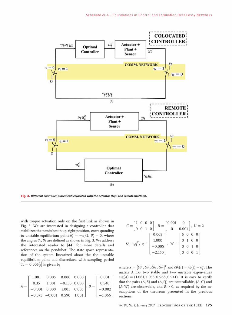
with torque actuation only on the first link as shown in
Fig. 3. We are interested in designing a controller that
stabilizes the pendubot in up-right position, corresponding
to unstable equilibrium point �1 ¼ �=2, �2 ¼ 0, where
the angles 1, 2 are defined as shown in Fig. 3. We address
the interested reader to [44] for more details andreferences on the pendubot. The state space representa-
tion of the system linearized about the the unstable
equilibrium point and discretized with sampling period
Ts ¼ 0:005½s� is given by
A ¼
1:001 0:005 0:000 0:000
0:35 1:001 �0:135 0:000
�0:001 0:000 1:001 0:005
�0:375 �0:001 0:590 1:001
2666437775; B ¼
0:001
0:540
�0:002
�1:066
2666437775
C ¼1 0 0 0
0 0 1 0
� �; R ¼
0:001 0
0 0:001
� �; U ¼ 2
Q ¼ qqT; q ¼
0:003
1:000
�0:005
�2:150
2666437775; W ¼
5 0 0 0
0 1 0 0
0 0 1 0
0 0 0 1
2666437775
where x ¼ ½�1; � _1; �2; � _2�T and �iðtÞ ¼ iðtÞ � �i . The
matrix A has two stable and two unstable eigenvalues
eigðAÞ ¼ ð1:061; 1:033; 0:968; 0:941Þ. It is easy to verify
that the pairs ðA; BÞ and ðA;QÞ are controllable, ðA; CÞ and
ðA;WÞ are observable, and R 9 0, as required by the as-
sumptions of the theorems presented in the previoussections.
Fig. 4. Different controller placement: colocated with the actuator (top) and remote (bottom).
Schenato et al. : Foundations of Control and Estimation Over Lossy Networks
Vol. 95, No. 1, January 2007 | Proceedings of the IEEE 175

We first compare the performance of the closed loopcontroller for two different control architecture, as shown
in Fig. 4. In the first scenario, we consider actuators with
no computational resources, therefore, the controller must
be implemented remotely and the control input is trans-
mitted to the actuator via a lossy communication link
which adopt a TCP-like protocol. We also assume that the
communication links between the sensors and the
controller and between the controller and the actuatorare independent and have the same arrival probability, i.e.,�� ¼ ��. In the second scenario, we consider the use of
Bsmart[ actuators, i.e., actuators with sufficient computa-
tional resources to implement the optimal controller. In
the scenario where the controller is colocated with the
actuator, it is equivalent to the TCP-like optimal control
with observation arrival probability ��eq ¼ ���� ¼ ��2 (series
of two independent lossy links) and control arrival pro-bability ��eq ¼ 1 (no communication link). Fig. 5 shows the
upper bound for the minimum infinite horizon cost Jmax1
defined in Theorem 5.6. The colocated controller clearly
outperforms the performance of the remote controller.
This is to be expected as the colocated controller can
compensate for observation packet with an optimal filter
and there is no control packet loss. The remote controller,on the other hand, can compensate only for the
observation packet loss, but not for the control packet
loss. Therefore, when practically feasible, it is always more
effective to place the controller as close as possible to the
actuators.
As a second example we compare the performance
under the TCP-like and UDP-like protocols, as shown in
Fig. 1. We consider the pendubot above with the ad-ditional assumptions of full state observation, i.e.,
C ¼ I4�4, and no sensor noise, i.e., R ¼ 04�4. Again we
assume independent lossy links with the same loss
probability �� ¼ ��. Fig. 6 shows the upper bound of
minimum cost Jmax1 under TCP-like protocols calculated as
in Theorem 5.6 and the minimum cost J�1 under UDP-
like protocols calculated as described in Theorem 8.5 in
the Appendix. The TCP-like communication protocolsgive better control performance than UDP-like, however
this comes at the price of an higher complexity in the
protocol design. Once again tradeoffs between perfor-
mance and complexity appear.
As a final example we consider a different compensa-
tion approach at the actuator site when no computational
Fig. 5. Upper bounds Jmax1 for the minimum cost with respect to two different controller locations under TCP-like protocols: controller
colocated with the actuator equivalent to TCP-like performance with ��eq ¼ ���� and ��eq ¼ 1 (thin solid line) and controller located remotely
from the actuator and connect by a communication network (thick solid line). Cost is calculated for �� ¼ ��.
Schenato et al.: Foundations of Control and Estimation Over Lossy Networks
176 Proceedings of the IEEE | Vol. 95, No. 1, January 2007

resources are available. In this paper, we chose to applyno control when a control packet is lost, ua
k ¼ 0. We call
this approach zero-input strategy. Another natural choice
is to use the previous control input if the current is lost, i.
e., uak ¼ ua
k�1 [15]. We call this second approach hold-
input strategy. Fig. 7 gives a pictorial representation of
these two strategies. We consider a very simple scalar
unstable system with parameters A ¼ 1:2, B ¼ C ¼ 1,
W ¼ U ¼ 1 and no process and measurement noise, i.e.,R ¼ Q ¼ 0. We also assume there is only control packet
loss with arrival probability �� ¼ 0:5 and no observation
packet loss, i.e., �� ¼ 1. Since there is no observation loss
and there is full state observation with no measurement
noise, the optimal control must necessarily be a static
feedback and no filter is necessary. The dynamics of the
closed loop with zero-input strategy can be written as
follows:
xkþ1 ¼ Axk þ Buak
uak ¼ �kuc
k
uck ¼ Lzxk (41)
and the dynamics for the hold-input strategy as
xkþ1 ¼ Axk þ Buak
uak ¼ �kuc
k þ ð1 � �kÞuak�1
uck ¼ Lhxk: (42)
We compare the performance in terms of the infinite
horizon expected total cost J1 ¼ E½P1
k¼0 x0kWxk þ ua0k Uua
k�.The optimal gain for the zero-input strategy can be com-
puted from (37) and is equal to L�z ¼ �1:02. However, the
exact computation of this expected cost for the hold-input
strategy cannot be computed analytically with the toolsdeveloped in this paper, therefore, we resort to the com-
putation of the empirical cost for a wide range of control
feedback gains Lz and Lz. Fig. 8 shows the empirical cost
Jemp1 computed as the average cost over 10 000 runs with
initial condition x0 ¼ 2, ua0 ¼ 0. Note that the empirical
optimal gain and the theoretical optimal gain L�z for the
zero-strategy are consistent. Surprisingly, the zero-input
strategy not only gives a comparable performance with thehold-input strategy but it appears to perform better both
Fig. 6. Minimum cost J1 under two different communication protocols: TCP-like (thin solid line) and UDP-like (thick solid line).
Schenato et al. : Foundations of Control and Estimation Over Lossy Networks
Vol. 95, No. 1, January 2007 | Proceedings of the IEEE 177

in terms of minimum achievable cost and in term of
robustness with respect to feedback gain sensitivity. This
is only an example and further rigorous analysis needs to
be performed to verify if this is a general result.
Nonetheless the zero-input strategy is a fair approach
and it is based on the rationale that in a stable closed loop
system driven by gaussian noise with zero mean, also the
input to the plant is gaussian with zero mean, therefore,
using uak ¼ 0 when a packet is lost is equivalent of using
an unbiased estimate of the input uck generated by the
remote controller.
VIII . CONCLUSION ANDFUTURE DIRECTIONS
In this paper, we have analyzed the LQG control problemin the case where both observation and control packets
may be lost during transmission over a communication
channel. This situation arises frequently in distributed
systems where sensors, controllers and actuators reside in
different physical locations and have to rely on data
networks to exchange information. We have presented
analysis of the LQG control problem under two classes of
protocols: TCP-like and UDP-like. In TCP-like protocols,
Fig. 7. Compensation approaches for actuators with no computational resources when a control packet is lost: zero-input approach
uak ¼ 0 (top) and hold-input approach ua
k ¼ uak�1 (bottom).
Schenato et al.: Foundations of Control and Estimation Over Lossy Networks
178 Proceedings of the IEEE | Vol. 95, No. 1, January 2007

acknowledgements of successful transmissions of control
packets are provided to the controller, while in UDP-like
protocols, no such feedback is provided.
For TCP-like protocols we have solved a general LQGcontrol problem in both the finite and infinite horizon
scenarios. We have shown that the optimal control is a
linear function of the state and that the separation
principle holds. As a consequence, controller design and
estimator design are decoupled under TCP-like protocols.
However, unlike standard LQG control with no packet
loss, the gain of the optimal observer does not converge to
a steady state value. Rather, the optimal observer gain is atime-varying stochastic function of the packet arrival
process. Several infinite horizon LQG controller design
methodologies proposed in the literature impose time-
invariance on the controller and are, therefore, subopti-
mal. In analyzing the infinite horizon problem, we have
shown that the infinite horizon cost is bounded if and only
if arrival probabilities ��, �� exceed a certain threshold.
Thus, the underlying communication channel must besufficiently reliable in order for LQG optimal controllers to
stabilize the plant.
UDP-like protocols present a much more complex
problem. We have shown that the lack of acknowledge-
ment of control packets results in the failure of the sepa-
ration principle. Estimation and control are now
intimately coupled. We have shown that the LQG optimal
control is, in general, nonlinear in the estimated state. As a
consequence, the optimal control law cannot be deter-mined explicitly in closed form, rendering this solution
impractical. In the special case where the state is com-
pleted observed (C is invertible and there is no output
noise i.e., R ¼ 0), the optimal control is indeed linear and
can be explicitly computed. We have shown that the set of
arrival probabilities ��, �� for which the infinite horizon cost
function is bounded, is smaller than the equivalent set for
TCP-like protocols. However, for moderate packet lossprobabilities the performance of these two classes of
protocols is comparable. This makes the simpler UDP-like
protocols attractive for networked control systems.
To fully exploit UDP-like protocols it is necessary to
have a controller/estimator design methodology for the
general case when there is measurement noise and under
partial state observation. Although the true LQG optimal
controller for UDP-like protocols is time-varying and hardto compute, we might choose to determine the optimal
time-invariant LQG controller. Although this is a subop-
timal strategy, this controller can be determined explicitly,
rendering implementation simple and computationally
effective, as recently presented in [45].
Fig. 8. Empirical cost for different values of the feedback gains Lz and Lh for the zero-input strategy (thin solid line)
and hold-input strategy (thick solid line).
Schenato et al. : Foundations of Control and Estimation Over Lossy Networks
Vol. 95, No. 1, January 2007 | Proceedings of the IEEE 179

We have shown that underlying communicationprotocols intimately affect the overall performance of
networked control systems. For example the separation
principle of LQG optimal control, a milestone in classical
control theory on which many modern controller design
techniques rest, does not hold in general for networked
control systems. This suggests that controller design needs
to be substantially reconsidered for such systems. A second
implication of our work is that controller design andcommunication protocol design are tightly coupled. This
suggests that communication protocols targeted to net-
worked control systems need to be developed. h
APPENDIXPROOFS
A. UDP-Like Special Case: R ¼ 0and C Invertible
Without loss of generality we can assume C ¼ I, sincethe linear transformation z ¼ Cx would give an equivalent
system where the matrix C is the indentity. Let us now
consider the case when there is no measurement noise,
i.e., R ¼ 0. These assumptions mean that it is possible to
measure the state xk when the observation packet is
delivered. In this case, the estimator (18)–(20) simplify
as follows:
Kkþ1 ¼ I (43)
Pkþ1jkþ1 ¼ð1 � �kþ1ÞPkþ1jk
¼ð1��kþ1Þ A0PkjkAþQ�
þ ��ð1���ÞBuku0kB0� (44)
E½Pkþ1jkþ1jGk�¼ ð1���Þ A0PkjkAþQ�þ ��ð1���ÞBuku0kB0� (45)
where in the last equation we used independence of �kþ1
and Gk, and we used the fact that Pkjk is a deterministic
function of Gk.
Following the same approach to optimal control
adopted in Section V, we claim that the value function
V�k ðxkÞ can be written as follows:
VkðxkÞ ¼ x̂0kjkSkx̂kjk þ traceðTkPkjkÞ þ traceðDkQÞ (46)
for k ¼ N; . . . ; 0. This is clearly true for k ¼ N, in fact
we have
VNðxNÞ ¼E x0NWNxNjGN
� ¼ x̂0NjNWNx̂NjN þ traceðWNPNjNÞ
where we used Lemma 4.1(b), therefore, the statement issatisfied by SN ¼ WN, TN ¼ WN, DN ¼ 0. Note that (46)
can be rewritten as follows:
VkðxkÞ¼E x0kSkxkjGk
� þ trace ðTk � SkÞPkjk
� �þ traceðDkQÞ
where we used once again Lemma 4.1(b). Moreover, to
simplify notation we define Hk ¼� ðTk � SkÞ. Let us suppose
that (46) is true for k þ 1 and let us show by induction it
holds true for k
VkðxkÞ ¼minuk
E x0kWkxk þ �ku0kUkuk þ Vkþ1ðxkþ1ÞjGk
� ¼min
uk
�E x0kWkxk þ �ku0kUkuk þ x0kþ1Skþ1xkþ1
�:
þ traceðHkþ1Pkþ1jkþ1Þþ traceðDkþ1QÞjGk�
�¼ E x0kðWk þ A0Skþ1AÞxkjGk
� þ traceðSkþ1QÞ þ ð1 � ��Þ� trace Hkþ1ðA0PkjkA þ QÞ
� �þ traceðDkþ1QÞ
þ minuk
��u0kUkuk þ ��u0kB0Skþ1Buk
�þ 2��u0kB0Skþ1Ax̂kjk þ ��ð1 � ��Þð1 � ��Þ� traceðHkþ1Buku0kB0Þ
�¼ E x0kðWk þ A0Skþ1AÞxkjGk
� þ trace Dkþ1 þ ð1 � ��ÞHkþ1ð ÞQð Þþ ð1 � ��ÞtraceðAHkþ1A0PkjkÞ þ traceðSkþ1QÞþ ��min
uk
u0k Uk þ B0 Skþ1 þ ð1 � ��Þðð�
� ð1 � ��ÞHkþ1ÞBÞ� uk þ 2u0kB0Skþ1Ax̂kjk
�¼ x̂0kjkðWk þ A0Skþ1AÞx̂kjk
þ trace Dkþ1 þ ð1 � ��ÞTkþ1 þ ��Skþ1ð ÞQð Þþ trace Wk þ ��A0Skþ1A þ ð1 � ��ÞATkþ1A0ð ÞPkjk
� �þ ��min
uk
u0k Uk þ B0 ð1 � ��ÞSkþ1 þ ��Tkþ1ð ÞBð Þuk
�þ 2u0kB0Skþ1Ax̂kjk
�;
where we defined �� ¼ ð1 � ��Þð1 � ��Þ, we usedLemma 4.1(c) to get the second equality, and (8) and
(45) to get the last equality. Since the quantity inside the
outer parenthesis is a convex quadratic function, the
minimizer is the solution of @Vk=@uk ¼ 0 which is given by
u�k ¼ � Uk þ B0 ð1 � ��ÞSkþ1 þ ��Tkþ1ð ÞBð Þ�1
� B0Skþ1Ax̂kjk (47)
¼ Lkx̂kjk (48)
Schenato et al.: Foundations of Control and Estimation Over Lossy Networks
180 Proceedings of the IEEE | Vol. 95, No. 1, January 2007

which is linear function of the estimated state x̂kjk.Substituting back into the value function we get
VkðxkÞ ¼ x̂0kjkðWk þ A0Skþ1AÞx̂kjk
þ trace Dkþ1 þ ð1 � ��ÞTkþ1 þ ��Skþ1ð ÞQð Þþ trace Wk þ A0Skþ1A þ ð1 � ��ÞATkþ1A0ð ÞPkjk
� �� ��x̂0kjkA0Skþ1BLkx̂kjk
¼ x̂0kjkðWk þ ��A0Skþ1A � ��x̂0kjkA0Skþ1BLkÞx̂kjk
þ trace Dkþ1 þ ð1 � ��ÞTkþ1 þ ��Skþ1ð ÞQð Þþ trace Wk þ A0Skþ1A þ ð1 � ��ÞATkþ1A0ð ÞPkjk
� �where we used Lemma 4.1(b) in the last equality. From the
last equation we see that the value function can be written
as in (46) if and only if the following equations are
satisfied:
Sk ¼ A0Skþ1A þ Wk � ��A0Skþ1B
� Uk þ B0 ð1 � ��ÞSkþ1 þ ��Tkþ1ð ÞBð Þ�1B0Skþ1A
¼SðSkþ1; Tkþ1Þ (49)
Tk ¼ð1 � ��ÞA0Tkþ1A þ ��A0Skþ1A þ Wk
¼TðSkþ1; Tkþ1Þ (50)
Dk ¼ð1 � ��ÞTkþ1 þ ��Skþ1 þ Dkþ1: (51)
The optimal minimal cost for the finite horizon,
J�N ¼ V0ðx0Þ is then given by
J�N ¼ x00S0x0 þ traceðS0P0Þ
þXN
k¼1
trace ð1 � ��ÞTk þ ��Skð ÞQð Þ: (52)
For the infinite horizon optimal controller, necessary
and sufficient conditions for the average minimal cost
J1 ¼� limN!þ1ð1=NÞJ�N to be finite, are that the coupled
iterative (49) and (50) should converge to a finite value S1and T1 as N ! þ1. In the work of Imer et al. [36],
similar equations were derived for the optimal LQG
control under UDP with the additional more stringentconditions Q ¼ 0 and B square and invertible. They
determine necessary and sufficient conditions for those
equations to converge. However, these conditions are
invalid in the general case when B in not square. Below we
prove a number of lemmas and theorems that will allow us
to derive stronger necessary and sufficient conditions even
when B not necessarily square and invertible.
Lemma 8.1: Let S, T 2 M ¼ fM 2 Rn�njM � 0g. Consi-
der the operators SðS; TÞ, and TðS; TÞ as defined in (49)
and (50), and consider the sequences Skþ1 ¼ SðSk; TkÞand Tkþ1 ¼ TðSk; TkÞ. Consider L�S;T ¼ �ðU þ B0ðð1���ÞS þ ��TÞBÞ�1B0SA and the operator:
ðS; T; LÞ ¼ 1 � ��
1 � ��
� �A0SA þ W
þ ��
1� ��A þ ð1 � ��ÞBLð Þ0S A þ ð1 � ��ÞBLð Þ
þ ��L0UL þ �� ��L0B0TBL
Then the following facts are true:
a) SðS; TÞ ¼ minL ðS; T; LÞb) 0 � ðS; T; L�S;TÞ ¼ SðS; TÞ � ðS; T; LÞ8Lc) If Skþ1 9 Sk and Tkþ1 9 Tk, then Skþ2 9 Skþ1 and
Tkþ2 9 Tkþ1.
d) If the pair ðA;W1=2Þ is observable and S ¼SðS; TÞ and T ¼ TðS; TÞ, then S 9 0 and T 9 0.
Proof:a) If U is invertible then it is easy to verify by direct
substitution substitution that
ðS; T; LÞ ¼SðS; TÞ þ �� L � L�S;T
�0� U þ B0 ð1 � ��ÞS þ ��Tð ÞBð Þ L � L�S;T
��SðS; TÞ
b) The nonnegativeness follows form the observation
that ðS; T; LÞ a sum of positive semi-definite
matrices. In fact, ð1 � ð��=ð1 � ��ÞÞÞ ¼ ð��ð1 � ��Þ=ð�� þ ��ð1 � ��ÞÞÞ � 0 and 0 � �� � 1. The equality
ðS; T; L�S;TÞ ¼ SðS; TÞ can be verified by direct
substitution. The last inequality follows directly
from Fact (b).
c)
Skþ2 ¼SðSkþ1; Tkþ1Þ ¼ Skþ1; Tkþ1; L�Skþ1;Tkþ1
�� Sk; Tk; L�Skþ1;Tkþ1
�� Sk; Tk; L�Sk;Tk
�¼SðSk; TkÞ ¼ Skþ1
Tkþ2 ¼TðSkþ1; Tkþ1Þ � TðSk; TkÞ ¼ Tkþ1
d) First observe that S ¼ SðS; TÞ � 0 and T ¼TðS; TÞ � 0. Thus, to prove that S, T 9 0, we
only need to establish that S, T are nonsingular.
Suppose they are singular, the there exist vectors
0 6¼ vs 2 NðSÞ and 0 6¼ vt 2 NðTÞ, i.e., Svs ¼ 0
Schenato et al. : Foundations of Control and Estimation Over Lossy Networks
Vol. 95, No. 1, January 2007 | Proceedings of the IEEE 181

and Tvt ¼ 0, where Nð�Þ indicates the null space.Then
0 ¼ v0sSvs ¼ v0sSðS; TÞvs ¼ v0s S; T; L�S;T
�vs
¼ 1 � ��
1 � ��
� �v0sA
0SAvs þ v0sWvs þ ?
where ? indicates other terms. Since all the terms
are positive semi-definite matrices, this implies
that all the term must be zero
v0sA0SAvs ¼ 0¼)SAvs ¼ 0¼)Avs 2 NðSÞ
v0sWvs ¼ 0¼)W1=2vs ¼ 0:
As a result, the null space NðSÞ is A-invariant.
Therefore, NðSÞ contains an eigenvector of A, i.e.,
there exists u 6¼ 0 such that Su ¼ 0 and Au ¼ �u.
As before, we conclude that Wu ¼ 0. This implies
(using the PBH test) that the pair ðA;W1=2Þ is notobservable, contradicting the hypothesis. Thus,
NðSÞ is empty, proving that S 9 0. The same
argument can be used to prove that also T 9 0. h
Lemma 8.2: Consider the following operator:
ðS; T; LÞ ¼ A0SA þ W þ 2��A0SBL
þ ��L0 U þ B0 ð1 � ��ÞS þ ��Tð ÞBð ÞL: (53)
Assume that the pairs ðA;W1=2Þ and ðA; BÞ are observable
and controllable, respectively. Then the following state-ments are equivalent:
a) There exist a matrix ~L and positive definite
matrices ~S and ~T such that
~S 9 0; ~T 9 0; ~S ¼ ð~S; ~T; ~LÞ; ~T ¼ Tð~S; ~TÞ:
b) Consider the sequences
Skþ1 ¼ SðSk; TkÞ; Tkþ1 ¼ TðSk; TkÞ
where the operators Sð�Þ, Tð�Þ are defined in
(49) and (50). For any initial condition S0, T0 � 0we have
limk!1
Sk ¼ S1; limk!1
Tk ¼ T1
and S1, T1 9 0 are the unique positive definitesolution of the following equations
S1 ¼ SðS1; T1Þ; T1 ¼ TðS1; T1Þ:
Proof:(a))(b) The main idea of the proof consists in proving
convergence of several monotonic sequences. Consider
t h e s e q u e n c e s Vkþ1 ¼ ðVk; Zk; ~LÞ a n d Zkþ1 ¼TðVk; ZkÞ with initial conditions V0 ¼ Z0 ¼ 0. It iseasy to verify by substitution that V1 ¼ W þ ��~L
0U~L �
0 ¼ V0 and Z1 ¼ W � 0 ¼ Z0. Lemma 8.1(a) shows
that the operator ðV; Z; ~LÞ is linear and monotonically
increasing in V and Z, i.e., ðVkþ1 � Vk; Zkþ1 � ZkÞ )ðVkþ2 � Vkþ1; Zkþ2 � Zkþ1Þ. Also the operator TðV; ZÞis linear and monotonically increasing in V and Z. Since
V1 � V0 and Z1 � Z0, using an induction argument we
have that Vkþ1 � Vk, Zkþ1 � Zk for all time k, i.e., thesequences are monotonically increasing. These se-
quences are also bounded, in fact ðV0 � ~SÞ; ðZ0 �~TÞ ) ðV1 ¼ ð0; 0; ~LÞ � ð~S; ~T; ~LÞ ¼ ~SÞ, ðZ1 ¼ Tð0;0Þ � Tð~S; ~TÞ ¼ ~TÞ and the same argument can be
inductively used to show that Vk � ~S and Zk � ~T for all
K. Consider now the sequences Sk, Tk as defined in the
theorem initialized with S0 ¼ T0 ¼ 0. By direct substi-
tution we find that S1 ¼ W � 0 ¼ S0 and T1 ¼ W �0 ¼ T0. By Lemma 8.1(c) follows that the sequences
Sk, Tk are monotonically increasing. Moreover, by
Lemma 8.1(b) it follows that ðSk � Vk; Tk � ZkÞ )ðSkþ1 ¼ SðSk; TkÞ � ðSk; Tk; ~LÞ � ðVk; Zk; ~LÞ ¼Vkþ1Þ, Tkþ1 ¼ TðSk; TkÞ � TðVk; ZkÞ¼ Zkþ1Þ. Since
this is verified for k ¼ 0, it inductively follows that
ðSk � Vk; Tk � ZkÞ for all k. Finally since Vk, Zk are
bounded, we have that (Sk � ~S, Tk � ~T. Since Sk, TkÞ aremonotonically increasing and bounded, it follows that
limk!1 Sk ¼ S1 and limk!1 Tk ¼ T1, where S1, T1are semi-definite matrices. From this it easily follows
that these matrices have the property S1 ¼SðS1; T1Þ, T1 ¼ TðS1; T1Þ. Definite positiveness
of S1 follows from Lemma 8.1(d) using the hypothesis
that ðA;W1=2Þ is observable. The same argument can be
used to prove that T1 9 0. Finally proof of uniquenessof solution and convergence for all initial conditions S0,
T0 can be obtained similarly to Theorem 1 in [37] and it
is, therefore, omitted.
(b))(a) This part follows easily by choosing~L ¼ L�S1;T1
, where L�S;T is defined in Lemma 8.1. Using
Lemma 8.1(b) we have S1 ¼ SðS1; T1Þ ¼ ðS1;T1; ~LÞ, therefore, the statement is verified using~S ¼ S1 and ~T ¼ T1. h
Lemma 8.3: Let us consider the fixed points of (49) and
(50), i.e., S ¼ SðS; TÞ, T ¼ TðS; TÞ where S, T � 0. Let
Schenato et al.: Foundations of Control and Estimation Over Lossy Networks
182 Proceedings of the IEEE | Vol. 95, No. 1, January 2007

A be unstable. A necessary condition for existence ofsolution is
jAj2ð�� þ �� � 2����Þ G �� þ �� � ���� (54)
where jAj ¼� maxi j�iðAÞj is the largest eigenvalue of the
matrix A.Proof: To prove the necessity condition it is sufficient
to show that there exist some initial conditions S0, T0 � 0
for which the sequences Skþ1 ¼ SðSk; TkÞ, Tkþ1 ¼TðSk; TkÞ are unbounded, i.e., limk!1 Sk ¼ limk!1 Tk ¼1. To do so, suppose that at some time-step k we have
Sk � skvv0 and Tk � tkvv0, where sk, tk 9 0, and v is the
eigenvector corresponding to the largest eigenvalue of A0,i.e., Av0 ¼ �maxv and j�maxj ¼ jA0j ¼ jAj. Then we have
Skþ1 ¼SðSk; TkÞ � Sðskvv0; tkvv0Þ
¼ minL
ðskvv0; tkvv0; LÞ
¼ minL
skA0vv0A þ W þ 2sk��A0vv0BLð
þ ��L0 U þ B0 ð1 � ��Þskvv0 þ ��tkvv0ð ÞBð ÞLÞ
� minL
skjAj2vv0 þ 2sk���maxvv0BL�þ ��L0B0 ð1 � ��Þskvv0 þ ��tkvv0ð ÞBÞLÞ
¼ minL
skjAj2vv0 � jAj2��s2k
�kvv0
�
þ ���k �maxs2kI þ 1
�kBL
� �0vv0
� �maxs2kI þ 1
�kBL
� ��
� skjAj2vv0 � jAj2��s2k
ð1 � ��Þsk þ ��tkvv0
¼ jAj2sk 1 � ��sk
ð1 � ��Þsk þ ��tk
� �vv0
¼ skþ1vv0
where I is the identity matrix and �k ¼ ð1 � ��Þsk þ ��tk.Similarly, we have
Tkþ1 ¼TðSk; TkÞ � Tðskvv0; tkvv0Þ
¼ ð1 � ��ÞtkA0vv0A þ ��skA0vv0A þ W
�ð1 � ��ÞtkjA2jvv0 þ ��skjAj2vv0
¼ jAj2 ð1 � ��Þtk þ ��skÞð Þvv0
¼ tkþ1vv0:
We can summarize the previous results as follows:
ðSk � skvv0; Tk � tkvv0Þ
) ðSkþ1 � skþ1vv0; Tkþ1 � tkþ1vv0Þ
skþ1 ¼ �sðsk; tkÞ ¼ jAj2sk 1 � ��sk
ð1 � ��Þsk þ ��tk
� �tkþ1 ¼ �tðsk; tkÞ ¼ jAj2 ð1 � ��Þtk þ ��skÞð Þ:
Let us define the following sequences:
Skþ1 ¼SðSk; TkÞ; Tkþ1 ¼ TðSk; TkÞ; S0 ¼ T0 ¼ vv0
skþ1 ¼�sðsk; tkÞ; tkþ1 ¼ �tðsk; tkÞ; s0 ¼ t0 ¼ 1
~Sk ¼ skvv0; ~Tk ¼ tkvv0:
From the previous derivations we have that Sk � ~Sk, Tk �~Tk for all time k. Therefore, it is sufficient to find when the
scalar sequences sk, tk diverges to find the necessary
conditions. It should be evident that also the operators�sðs; tÞ, �tðs; tÞ are monotonic in their arguments. Also it
should be evident that the only fixed points of s ¼ �sðs; tÞ,t ¼ �tðs; tÞ are s ¼ t ¼ 0. Therefore, we should be find
when the origin is an unstable equilibrium point, since in
this case limk!1 sk, tk ¼ 1. Note that t ¼ �tðs; tÞ can be
written as
t ¼Tðs; tÞ ¼ ð1 � ��ÞjAj2t þ ��jAj2s
¼ ðsÞ ¼ ��jAj2s
1 � ð1 � ��ÞjAj2
with the additional constraint 1 � ð1 � ��ÞA2 9 0. A neces-
sary condition for stability for the origin is that the origin of
A necessary condition for stabilityis jAj2ð�� þ �� � 2����Þ G ð�� þ �� � ����Þ:
Schenato et al. : Foundations of Control and Estimation Over Lossy Networks
Vol. 95, No. 1, January 2007 | Proceedings of the IEEE 183

restricted map zkþ1 ¼ �ðzk; ðzkÞÞ is stable. The restrictedmap is given by
zkþ1 ¼ jAj2zk 1 � ��zk
ð1 � ��Þzk þ �� ��jAj21�ð1���ÞA2 zk
0@ 1A¼ jAj2 1 � ��
ð1 � ��Þ þ �� ��jAj21�ð1���ÞA2
0@ 1Azk
¼ jAj2 1 ��� 1 � ð1 � ��ÞjAj2� �
�� þ �� � ���� � ��ð1 � ��ÞjAj2
!zk
¼ ��ð1 � ��ÞjAj2
�� þ �� � ���� � ��ð1 � ��ÞjAj2
!zk:
This is a linear map and it is stable only if the term inside
the parenthesis is smaller than unity, i.e.,
��ð1 � ��ÞjAj2
�� þ �� � ���� � ��ð1 � ��ÞjAj2
!G 1
�� þ �� � ���� � ��ð1 � ��ÞjAj2 9 ��ð1 � ��ÞjAj2
�� þ �� � ���� 9 jAj2ð�� þ �� � 2����Þ
which concludes the lemma. h
Lemma 8.4: Let us consider the fixed points of (49) and
(50), i.e., S ¼ SðS; TÞ, T ¼ TðS; TÞ where S, T � 0. Let Abe unstable, ðA;W1=2Þ observable and B square and invert-ible. Then a sufficient condition for existence of solution is
jAj2ð�� þ �� � 2����Þ G �� þ �� � ���� (55)
where jAj ¼� maxi j�iðAÞj is the largest eigenvalue of the
matrix A.
Proof: The proof is constructive. In fact, we find a
control feedback gain ~L that satisfies the conditions stated
in Theorem 8.2(a). Let ~L ¼ ��B�1A where � 9 0 is a
positive scalar that is to be determined. Also consider
S ¼ sI, T ¼ tI, where I is the identity matrix and s, t 9 0
are positive scalars. Then, we have
ðsI; tI; ~LÞ ¼ A0sAþW�2���A0sA
þ ��A0B�0UB�1Aþ���2A0 ð1� ��Þsþ ��tð ÞA
� jAj2 s�2��s�þ�� ð1� ��Þsþ ��tð Þ�2� �
IþwI
¼’sðs; t; �ÞI (56)
TðsI; tIÞ ¼ ��A0sAþð1���ÞA0tAþW
� ��jAj2sþð1���ÞjAj2t� �
IþwI
�’tðs; tÞI (57)
where w ¼ jW þ ��A0B�0UB�1Aj 9 0 and I is the identity
matrix. Let us consider the following scalar operators and
sequences:
’sðs; t; �Þ ¼ jAj2 1 � 2��� þ ��ð1 � ��Þ�2� �
s þ �� ���2t þ w
’tðs; tÞ ¼ ��jAj2s þ ð1 � ��ÞjAj2t þ w
skþ1 ¼’sðsk; tk; �Þ; tkþ1 ¼ ’tðsk; tkÞ; s0 ¼ t0 ¼ 0:
The operators are clearly monotonically increasing in
s, t, and since s1 ¼ ’sðs0; t0; �Þ ¼ w � s0 and t1 ¼’tðs0; t0Þ ¼ w � t0, it follows that the sequences sk, tk
are monotonically increasing. If these sequences are
bounded, then they must converge to ~s, ~t. Therefore, sk,
tk are bounded if and only if there exist ~s, ~t 9 0 such that
~s ¼ ’sð~s;~t; �Þ and ~t ¼ ’tð~s;~tÞ. Let us find the fixed points
~t ¼’tð~s;~tÞ )
~t ¼ ��jAj2
1 � ð1 � ��ÞjAj2~s þ wt
where wt ¼� ðw=ð1 � ð1 � ��ÞjAj2ÞÞ 9 0, and we must have
1 � ð1 � ��ÞjAj2 9 0 to guarantee that ~t 9 0. Substituting
back into the operator ’s we have
~s ¼jAj2 1 � 2��� þ ��ð1 � ��Þ�2� �
~s þ �� ���2 ��jAj2
1 � ð1 � ��ÞjAj2~s
þ �� ���2wt þ w
¼jAj2
1 � 2��� þ ��
� ð1 � ��Þ þ �� ��jAj2
1 � ð1 � ��ÞjAj2
!�2
!~s þ wð�Þ
¼jAj2
1 � 2���
þ ���� þ �� � ���� � ��ð1 � ��ÞjAj2
1 � ð1 � ��ÞjAj2�2
!~s þ wð�Þ
¼að�Þ~s þ wð�Þ
where wð�Þ ¼� �� ���2wt þ w 9 0. For a positive solution ~sto exist, we must have að�Þ G 1. Since að�Þ is a
quadratic function of the free parameter �, we can try
to increase the basin of existence of solutions by
Schenato et al.: Foundations of Control and Estimation Over Lossy Networks
184 Proceedings of the IEEE | Vol. 95, No. 1, January 2007

choosing �� ¼ arg min� að�Þ, which can be found bysolving ðda=d�Þð��Þ ¼ 0 and is given by
�� ¼ 1 � ð1 � ��ÞjAj2
�� þ �� � ���� � ��ð1 � ��ÞjAj2:
Therefore, a sufficient condition for existence of solutions
is given by
að��Þ G 1
jAj2 1 � ��1 � ð1 � ��ÞjAj2
�� þ �� � ���� � ��ð1 � ��ÞjAj2
!G 1
��ð1 � ��ÞjAj2
�� þ �� � ���� � ��ð1 � ��ÞjAj2
!G 1
which is the same bound for the necessary condition of
convergence in Lemma 8.3.
If this condition is satisfied, then limk!1 sk ¼ ~s and
limk!1 tk ¼ ~t. Let us consider now the sequences �Sk ¼ skI,�Tk ¼ tkI, Skþ1 ¼ ðSk; Tk; ~LÞ, and Tkþ1 ¼ TðSk; TkÞ where~L ¼ ���B�1A, S0 ¼ T0 ¼ 0, and sk, tk where defined
above. These sequences are all monotonically increasing.From (56) and (57), it follows that ðSk � skI; Tk � tkIÞ )ðSkþ1 ¼� skþ1I; Tkþ1 � tkIÞ. Since this is verified for k ¼ 0
we can claim that Sk G ~sI and Tk G ~tI for all k. Since Sk, Tk
are monotonically increasing and bounded, then they must
converge to positive semidefinite matrices ~S, ~T � 0 which
solve the equations ~S ¼ ð~S; ~T; ~LÞ and ~T ¼ Tð~S; ~TÞ. Since
by hypothesis the pair ðA;W1=2Þ is observable, using
similar arguments of Lemma 8.1(d), it is possible to showthat ~S, ~T 9 0. Therefore, ~S, ~T, ~L satisfy the conditions of
Theorem 8.2(a), from which if follows statement (b) of the
same theorem. This implies that the sufficient conditions
derived here guarantee the claim of the lemma. hWe can use the previous lemmas to prove the following
theorems that states the properties of optimal control for
UDP-like protocols in the special scenario with no
measurement noise and full state observation.
Theorem 8.5: Consider the system (1)–(3) and considerthe problem of minimizing the cost function (5) within the
class of admissible policies uk ¼ fðGkÞ, where Gk is the
information available under UDP-like schemes, given in
(4). Assume also that R ¼ 0 and C is square and invertible.
Then:
a) The optimal estimator gain is constant and in
particular Kk ¼ I if C ¼ I.b) The infinite horizon optimal control exists if and
only if there exists positive definite matrices S1,
T1 9 0 such that S1 ¼ SðS1; T1Þ and T1 ¼TðS1; T1Þ, where S and S are defined in (49)
and (50).
c) The infinite horizon optimal controller gain is
constant
limk!1
Lk ¼ L1
L1 ¼ � B0 ��T1 þ ð1 � ��ÞS1ð ÞB þ Uð Þ�1
� B0S1A: (58)
d) A necessary condition for existence of S1,
T1 9 0 is
jAj2ð�� þ �� � 2����Þ G �� þ �� � ���� (59)
where jAj ¼� maxi j�iðAÞj is the largest eigenvalue
of the matrix A. This condition is also sufficient if
B is square and invertible.
e) The expected minimum cost for the infinite
horizon scenario converges to
J�1 ¼ limk!1
1
NJ�N
¼ trace ð1 � ��ÞT1 þ ��S1ÞQð Þ: (60)
Proof: (a) This fact follows from (43)–(45).Statements (b), (c), and (e) follow from Lemma 8.2
and (47) and (52). Statement (d) corresponds to
Lemmas 8.3 and 8.4. h
RE FERENCES
[1] I. A. W. Su, Y. Sankarasubramaniam, andE. Cayirci, BA survey on sensor networks,[IEEE Commun. Mag., vol. 40, no. 8,pp. 102–116, Aug. 2002.
[2] D. Estrin, D. Culler, K. Pister, andG. Sukhatme, BConnecting the physical worldwith pervasive networks,[ IEEE PervasiveComputing, vol. 1, no. 1, pp. 59–69, Jan. 2002.
[3] Proc. IEEE (Special Issue on Sensor Networksand Applications), vol. 91, no. 8,pp. 1151–1256, Aug. 2003.
[4] J. Wills, BWill HVAC control go wireless?[ASHRAE J., vol. 46, no. 7, pp. 46–50,Jul. 2004.
[5] M. Kintner-Meyer and R. Conant,BOpportunities of wireless sensors andcontrols for building operation,[ Energ.Eng. J., vol. 102, no. 5, pp. 27–48, 2005.
[6] B. Warneke, M. Last, B. Leibowitz, andK. Pister, BSmart dust: Communicating witha cubic-millimeter computer,[ Computer,vol. 34, no. 1, pp. 44–51, Jan. 2001.
[7] S. Boyer, SCADA: Supervisory Control andData Acquisition, ISA-The Instrumentation,Systems, and Automation Society2004.
[8] D. Bailey, Practical SCADA for Industry.Burlington, MA: Newnes, 2003.
[9] A. L. Sangiovanni-Vincentelli, BElectronic-system design in the automobile industry,[IEEE Microw Mag., vol. 21, no. 3, pp. 8–18,May 2003.
[10] G. Leen and D. Heffernan, BExpandingautomotive electronic systems,[ Computer,vol. 35, no. 1, pp. 88–93, 2002.
Schenato et al. : Foundations of Control and Estimation Over Lossy Networks
Vol. 95, No. 1, January 2007 | Proceedings of the IEEE 185

[11] V. Gupta, D. Spanos, B. Hassibi, andR. M. Murray, BOptimal LQG control across apacket-dropping link,[ Systems Control Lett.2005.
[12] Y. Xu and J. Hespanha, BEstimation undercontrolled and uncontrolled communicationsin networked control systems,[ in Proc. IEEEConf. Decision and Control, Sevilla, Spain,Dec. 2005, pp. 842–847.
[13] S. Smith and P. Seiler, BEstimation with lossymeasurements: Jump estimators for jumpsystems,[ IEEE Trans. Autom. Control, vol. 48,no. 12, pp. 1453–1464, Dec. 2003.
[14] J. Nilsson, B. Bernhardsson, andB. Wittenmark, BStochastic analysis andcontrol of real-time systems with random timedelays,[ Automatica, vol. 34, no. 1, pp. 57–64,Jan. 1998.
[15] J. Nilsson, BReal-time control systems withdelays,[ Ph.D. dissertation, Dept. AutomaticControl, Lund Inst. Technol., Lund, Sweden,1998.
[16] C. N. Hadjicostis and R. Touri, BFeedbackcontrol utilizing packet dropping networklinks,[ in Proc. IEEE Conf. Decision andControl, Las Vegas, NV, Dec. 2002, vol. 2,pp. 1205–1210.
[17] Q. Ling and M. Lemmon, BOptimal dropoutcompensation in networked control systems,[presented at the IEEE Conf. Decision andControl, Maui, HI, Dec. 2003.
[18] N. Yu, L. Wang, G. Xie, and T. Chu,BStabilization of networked control systemswith data packet dropout via swithed systemapproach,[ in IEEE Int. Symp. Computer AidedControl Systems Design, Taipei, Taiwan,Sep. 2004, pp. 362–367.
[19] P. Seiler and R. Sengupta, BAn H1 approachto networked control,[ IEEE Trans. Autom.Control, vol. 50, no. 3, pp. 356–364,Mar. 2005.
[20] A. V. Savkin and I. R. Petersen, BRobustfiltering with missing data and a deterministicdescription of noise and uncertainty,[ Int. J.Syst. Sci., vol. 28, no. 4, pp. 373–390, 1997.
[21] J. do Val, J. Geromel, and O. Costa, BSolutionsfor the linear quadratic control problem ofmarkov jump linear systems,[ J. OptimizationTheory Appl., vol. 103, no. 2, pp. 283–311,1999.
[22] O. Costa, BStationary filter for linearminimum mean square error estimator ofdiscrete-time markovian jump systems,[
Trans. Autom. Control, vol. 48, no. 8,pp. 1351–1356, Aug. 2002.
[23] Z. Wang, D. Ho, and X. Liu,BVariance-constrained control for uncertainstochastic systems with missingmeasurements,[ IEEE Trans. Syst., Man,Cybern. A: Syst. Humans, vol. 35, no. 5,pp. 746–753, Sep. 2005.
[24] N. Elia and J. Eisembeis, BLimitation of linearcontrol over packet drop networks,[ in Proc.IEEE Conf. Decision and Control, Bahamas,Dec. 2004, vol. 5, pp. 5152–5157.
[25] N. Elia, BRemote stabilization over fadingchannels,[ Syst. Control Lett., vol. 54,pp. 237–249, 2005.
[26] W. S. Wong and R. W. Brockett,BSystems with finite communicationbandwidth constraints. II. Stabilization withlimited information feedback,[ IEEE Trans.Autom. Contr., vol. 44, no. 5, pp. 1049–1053,May 1999.
[27] N. Elia and S. Mitter, BStabilization of linearsystems with limited information,[ IEEETrans. Autom. Contr., vol. 46, no. 9,pp. 1384–1400, Sep. 2001.
[28] J. P. Hespanha, A. Ortega, and L. Vasudevan,BTowards the control of linear systems withminimum bit-rate,[ in Proc. Int. Symp.Mathematical Theory of Networks and Systems,2002, pp. 1–15.
[29] G. N. Nair and R. J. Evans, BExponentialstabilisability of finite dimensional linearsystems with limited data rates,[Automatica, vol. 39, no. 4, pp. 585–593,Apr. 2003.
[30] S. Tatikonda and S. Mitter, BControl undercommunication constraints,[ IEEE Trans.Autom. Contr., vol. 49, no. 7, pp. 1056–1068,Jul. 2004.
[31] J. H. Braslavsky, R. H. Middleton, andJ. S. Freudenberg, BFeedback stabilizationover signal-to-noise ratio constrainedchannels,[ in Proc. 2004 American ControlConf., Jun. 2004, pp. 4903–4908.
[32] N. Martins, M. Dahleh, and N. Elia,BFeedback stabilization of uncertain systemsusing a stochastic digital link,[ in Proc. IEEEConf. Decision and Control, Dec. 2004, vol. 2,pp. 1889–1895.
[33] S. Yuksel and T. Basar, BMinimum rate codingfor state estimation over noiseless channels,[in Proc. IEEE Conf. Decision and Control, 2004,pp. 4503–4508.
[34] D. Liberzon and J. P. Hespanha, BStabilizationof nonlinear systems with limited informationfeedback,[ IEEE Trans. Autom. Contr., vol. 50,no. 6, pp. 910–915, Jun. 2005.
[35] A. Sahai and S. Mitter, BThe necessity andsufficiency of anytime capacity for controlover a noisy communication link: Part I scalarsystems,[ IEEE Trans. Inf. Theory, vol. 52,no. 8, pp. 3369–3395, Aug. 2006.
[36] O. C. Imer, S. Yuksel, and T. Basar, BOptimalcontrol of dynamical systems over unreliablecommunication links,[ Automatica, vol. 42,no. 9, pp. 1429–1439, Sep. 2006.
[37] B. Sinopoli, L. Schenato, M. Franceschetti,K. Poolla, M. Jordan, and S. Sastry, BKalmanfiltering with intermittent observations,[IEEE Trans. Autom. Contr., vol. 49, no. 9,pp. 1453–1464, Sep. 2004.
[38] X. Liu and A. Goldsmith, BKalman filteringwith partial observation losses,[ in Proc.IEEE Conf. Decision and Control, Bahamas,Dec. 2004, vol. 4, pp. 4180–4186.
[39] B. Sinopoli, L. Schenato, M. Franceschetti,K. Poolla, M. Jordan, and S. Sastry, BOptimalcontrol with unreliable communication:The TCP case,[ in Proc. American ControlConf., Portland, OR, Jun. 2005, vol. 5,pp. 3354–3359.
[40] D. Bertsekas and J. Tsitsiklis, Neuro-DynamicProgramming. Nashua, NH: AthenaScientific, Sep. 1996.
[41] G. Chen, G. Chen, and S. Hsu, LinearStochastic Control Systems. Boca Raton, FL:CRC Press, 1995.
[42] T. Katayama, BOn the matrix Riccati equationfor linear systems with a random gain,[ IEEETrans. Autom. Control, vol. AC-21, no. 2,pp. 770–771, Oct. 1976.
[43] W. Koning, BInfinite horizon optimal controlfor linear discrete time systems withstochastic parameters,[ Automatica, vol. 18,no. 4, pp. 443–453, 1982.
[44] M. Zhang and T.-J. Tarn, BHybrid controlof the pendubot,[ IEEE/ASME Trans.Mechatron., vol. 7, no. 1, pp. 79–86,2002.
[45] B. Sinopoli, L. Schenato, M. Franceschetti,K. Poolla, M. Jordan, and S. Sastry, BOptimallinear LQG control over lossy networkswithout packet acknowledgment,[ presentedat the IEEE Conf. Decision and Control, SanDiego, CA, Dec. 2006.
ABOUT THE AUT HORS
Luca Schenato (Member, IEEE) received the Dr.
Eng. degree in electrical engineering from the
University of Padova, Padova, Italy, in 1998 and
the Ph.D. degree in electrical engineering and
computer sciences from the University of
California at Berkeley (U.C. Berkeley), in 2003.
From January 2004 till August 2004, he was a
postdoctoral scholar at U.C. Berkeley. Since then
he has been with the Control Systems Group in the
Department of Information Engineering at the
University of Padova where he is Adjunct Professor. His interests include
networked control systems, wireless sensor networks, distributed
control, swarm robotics, and biomimetic locomotion.
Dr. Schenato was awarded the 2004 Researchers Mobility Fellowship
by the Italian Ministry of Education, University and Research (MIUR), and,
jointly with Dr. B. Sinopoli, the 2006 Eli Jury Award at U.C. Berkeley for
outstanding research achievement in the area of systems, communica-
tions, control, and signal processing.
Bruno Sinopoli (Member, IEEE) received the Dr.
Eng. degree from the University of Padova,
Padova, Italy, in 1998. He received the M.S. and
Ph.D. degrees in electrical engineering from
the University of California at Berkeley (U.C.
Berkeley), in 2003 and 2005, respectively.
He currently holds a joint postdoctoral ap-
pointment in the departments of Electrical Engi-
neering both at Stanford University, Stanford, CA,
and at the U.C. Berkeley. His research interests
include networked embedded control systems, distributed estimation
and control, and hybrid systems with applications to wireless sensor-
actuator networks.
Dr. Sinopoli was awarded, jointly with Dr. L. Schenato, the 2006 Eli
Jury Award for outstanding research achievement in the areas of
systems, communications, control and signal processing at U.C. Berkeley.
Schenato et al.: Foundations of Control and Estimation Over Lossy Networks
186 Proceedings of the IEEE | Vol. 95, No. 1, January 2007
Massimo Franceschetti (Member, IEEE) received
the Laurea degree (magna cum laude) in computer
engineering from the University of Naples, Naples,
Italy, in 1997, and the M.S. and Ph.D. degrees in
electrical engineering from the California Institute
of Technology, Pasadena, in 1999 and 2003.
He is an Assistant Professor in the Department
of Electrical and Computer Engineering, University
of California at San Diego. Before joining UCSD, he
was a postdoctoral scholar at University of
California at Berkeley for two years. He has held visiting positions at
the Vrije Universiteit Amsterdam in the Netherlands, the Ecole
Polytechnique Federale de Lausanne in Switzerland, and the University
of Trento in Italy. His research interests include random networks for
communication, wave propagation in random media, and control over
networks. He is currently associate guest co-editor of the IEEE
TRANSACTIONS ON INFORMATION THEORY, special issue on relay and cooper-
ation in networks.
Prof. Franceschetti was awarded the C.H. Wilts Prize in 2003 for best
doctoral thesis in Electrical Engineering at Caltech; the S.A. Schelkunoff
award in 2005 (jointly with Prof. J. Bruck and Prof. L. J. Shulman) for best
paper in the IEEE TRANSACTIONS ON ANTENNAS AND PROPAGATION; and an NSF
CAREER award in 2006.
Kameshwar Poolla received the Bachelor of
Technology degree from the Indian Institute of
Technology, Bombay, India, in 1980, and the Ph.D.
degree from the University of Florida, Gainesville
in 1984.
He has served on the faculty of the Department
of Electrical and Computer Engineering at the
University of Illinois, Urbana, from 1984 to 1991.
Since then, he has been with the University of
California, Berkeley, where he is a Professor of
Mechanical Engineering and Electrical Engineering & Computer Sciences.
He has also held visiting appointments at Honeywell, McGill University,
M.I.T., Michigan, and Columbia, and has worked as a Field Engineer with
Schlumberger on oilrigs in West Africa. In 1999, he co-founded On Wafer
Technologies which offers metrology-based yield-enhancement solu-
tions for the semiconductor industry, where he currently serves as Chief
Scientist. His research interests include micro-sensors, system identifi-
cation, robust control, semiconductor manufacturing, and medical
imaging.
Prof. Poolla was awarded a 1988 NSF Presidential Young Investigator
Award, the 1993 Hugo Schuck Best Paper Prize, the 1994 Donald P.
Eckman Award, the 1998 Distinguished Teaching Award of the University
of California, and the 2005 IEEE TRANSACTIONS ON SEMICONDUCTOR
MANUFACTURING Best Paper Prize.
S. Shankar Sastry (Fellow, IEEE) received the M.S.
degree (honoris causa) from Harvard University,
Cambridge, MA, in 1994, and the Ph.D. degree
from the University of California, Berkeley, in 1981.
From 1980 to 1982, he was an Assistant Pro-
fessor at Massachusetts Institute of Technology,
Cambridge. In 2000, he was Director of the
Information Technology Office at the Defense
Advanced Research Projects Agency, Arlington,
VA, and Chairman of the Department of Electrical
Engineering and Computer Sciences, University of California, Berkeley.
He is currently the NEC Distinguished Professor of Electrical Engineering
and Computer Sciences and Bioengineering, and the Director of the
Center for Information Technology Research in the Interest of Society,
University of California, Berkeley.
His research interests are embedded and autonomous software,
computer vision, computation in novel substrates such as DNA, nonlinear
and adaptive control, robotic telesurgery, control of hybrid systems,
embedded systems, sensor networks, and biological motor control.
Dr. Sastry was elected into the National Academy of Engineering in
2000 Bfor pioneering contributions to the design of hybrid and
embedded systems.[ He has served as Associate Editor for IEEE
TRANSACTIONS ON AUTOMATIC CONTROL, IEEE Control Systems Magazine,
and IEEE TRANSACTIONS ON CIRCUITS AND SYSTEMS.
Schenato et al. : Foundations of Control and Estimation Over Lossy Networks
Vol. 95, No. 1, January 2007 | Proceedings of the IEEE 187