Embed Size (px)
Citation preview
IEEE TRANSACTIONS ON AUDIO, SPEECH, AND LANGUAGE PROCESSING, VOL. 14, NO. 2, MARCH 2006 679
A Generative Model for Music TranscriptionA. Taylan Cemgil, Member, IEEE, Hilbert J. Kappen, Senior Member, IEEE, and David Barber
Abstract—In this paper, we present a graphical model for poly-phonic music transcription. Our model, formulated as a dynamicalBayesian network, embodies a transparent and computationallytractable approach to this acoustic analysis problem. An advantageof our approach is that it places emphasis on explicitly modelingthe sound generation procedure. It provides a clear framework inwhich both high level (cognitive) prior information on music struc-ture can be coupled with low level (acoustic physical) informationin a principled manner to perform the analysis. The model is aspecial case of the, generally intractable, switching Kalman filtermodel. Where possible, we derive, exact polynomial time inferenceprocedures, and otherwise efficient approximations. We argue thatour generative model based approach is computationally feasiblefor many music applications and is readily extensible to more gen-eral auditory scene analysis scenarios.
Index Terms—Bayesian signal processing, music transcription,polyphonic pitch tracking, switching Kalman filters.
I. INTRODUCTION
WHEN HUMANS listen to sound, they are able toassociate acoustical signals generated by different
mechanisms with individual symbolic events [1]. The studyand computational modeling of this human ability forms thefocus of computational auditory scene analysis (CASA) andmachine listening [2]. Research in this area seeks solutions toa broad range of problems such as the cocktail party problem,(for example automatically separating voices of two or moresimultaneously speaking persons, see, e.g., [3] and [4]), identi-fication of environmental sound objects [5] and musical sceneanalysis [6]. Traditionally, the focus of most research activitieshas been in speech applications. Recently, analysis of musicalscenes is drawing increasingly more attention, primarily be-cause of the need for content based retrieval in very large digitalaudio databases [7] and increasing interest in interactive musicperformance systems [8].
A. Music Transcription
One of the hard problems in musical scene analysis is au-tomatic music transcription, that is, the extraction of a humanreadable and interpretable description from a recording of a
Manuscript received January 19, 2004; revised August 23, 2004. This worksupported by the Technology Foundation STW, Applied Science Division ofNWO, and the Technology Programme of the Dutch Ministry of Economic Af-fairs. The Associate Editor coordinating the review of this manuscript and ap-proving it for publication was Dr. Michael Davies.
A. T. Cemgil is with Stichting Neurale Netwerken, SNN, 6525 EZ Nimegen,The Netherlands, and also with the Informatics Institute, University of Ams-terdam, 1098 SJ Amsterdam, The Netherlands (e-mail: [email protected]).
H. J. Kappen is with the Radboud University Nijmegen, 6525 EZ Nijmegen,The Netherlands (e-mail: [email protected]).
D. Barber is with the IDIAP, CH-1920 Martigny, Switzerland (e-mail:[email protected]).
Digital Object Identifier 10.1109/TSA.2005.852985
music performance. Ultimately, we wish to infer automatically amusical notation (such as the traditional western music notation)listing the pitch levels of notes and corresponding time-stampsfor a given performance. Such a representation of the surfacestructure of music would be very useful in a broad spectrumof applications such as interactive music performance systems,music information retrieval (Music-IR) and content descriptionof musical material in large audio databases, as well as in theanalysis of performances. In its most unconstrained form, i.e.,when operating on an arbitrary polyphonic acoustical input pos-sibly containing an unknown number of different instruments,automatic music transcription remains a great challenge. Ouraim in this paper is to consider a computational framework tomove us closer to a practical solution of this problem.
Music transcription has attracted significant research effortin the past—see [6] and [9] for a detailed review of early andmore recent work, respectively. In speech processing, the re-lated task of tracking the pitch of a single speaker is a fun-damental problem and methods proposed in the literature arewell studied [10]. However, most current pitch detection algo-rithms are based largely on heuristics (e.g., picking high energypeaks of a spectrogram, correlogram, auditory filter bank, etc.)and their formulation usually lacks an explicit objective func-tion or signal model. It is often difficult to theoretically justifythe merits and shortcomings of such algorithms, and comparethem objectively to alternatives or extend them to more com-plex scenarios.
Pitch tracking is inherently related to the detection and esti-mation of sinusoids. The estimation and tracking of single ormultiple sinusoids is a fundamental problem in many branchesof applied sciences, so it is less surprising that the topic has alsobeen deeply investigated in statistics, (e.g., see [11]). However,ideas from statistics seem to be not widely applied in the contextof musical sound analysis, with only a few exceptions [12], [13]who present frequentist techniques for very detailed analysis ofmusical sounds with particular focus on decomposition of pe-riodic and transient components. [14] has presented real-timemonophonic pitch tracking application based on a Laplace ap-proximation to the posterior parameter distribution of an AR(2)model [15], [11, p. 19]. Their method outperforms several stan-dard pitch tracking algorithms for speech, suggesting potentialpractical benefits of an approximate Bayesian treatment. Formonophonic speech, a Kalman filter based pitch tracker is pro-posed by [16] that tracks parameters of a harmonic plus noisemodel (HNM). They propose the use of Laplace approximationaround the predicted mean instead of the extended Kalman filter(EKF). For both methods, however, it is not obvious how to ex-tend them to polyphony.
Kashino [17] is, to our knowledge, the first author to applygraphical models explicitly to the problem of polyphonic music
1558-7916/$20.00 © 2006 IEEE
680 IEEE TRANSACTIONS ON AUDIO, SPEECH, AND LANGUAGE PROCESSING, VOL. 14, NO. 2, MARCH 2006
transcription. Sterian [18] described a system that viewedtranscription as a model driven segmentation of a time-fre-quency image. Walmsley [19] treats transcription and sourceseparation in a full Bayesian framework. He employs a framebased generalized linear model (a sinusoidal model) and pro-poses inference by reversible-jump Markov Chain Monte Carlo(MCMC) algorithm. The main advantage of the model is thatit makes no strong assumptions about the signal generationmechanism, and views the number of sources as well as thenumber of harmonics as unknown model parameters. Davy andGodsill [20] address some of the shortcomings of his modeland allow changing amplitudes and frequency deviations.The reported results are encouraging, although the method iscomputationally very expensive.
B. Approach
Musical signals have a very rich temporal structure, both ona physical (signal) and a cognitive (symbolic) level. From a sta-tistical modeling point of view, such a hierarchical structure in-duces very long range correlations that are difficult to capturewith conventional signal models. Moreover, in many music ap-plications, such as transcription or score following, we are usu-ally interested in a symbolic representation (such as a score)and not so much in the “details” of the actual waveform. Toabstract away from the signal details, we define a set of inter-mediate variables (a sequence of indicators), somewhat analo-gous to a “piano-roll” representation. This intermediate layerforms the “interface” between a symbolic process and the ac-tual signal process. Roughly, the symbolic process describeshow a piece is composed and performed. We view this processas a prior distribution on the piano-roll. Conditioned on thepiano-roll, the signal process describes how the actual wave-form is synthesized.
Most authors view automated music transcription asan “audio to piano-roll” conversion and usually consider“piano-roll to score” a separate problem. This view is partiallyjustified, since source separation and transcription from apolyphonic source is already a challenging task. On the otherhand, automated generation of a human readable score includesnontrivial tasks such as tempo tracking, rhythm quantization,meter and key induction [21]–[23]. As also noted by otherauthors (e.g., [17], [24], and [25]), we believe that a model thatintegrates this higher level symbolic prior knowledge can guideand potentially improve the inferences, both in terms quality ofa solution and computation time.
There are many different natural generative models for piano-rolls. In [26], we proposed a realistic hierarchical prior model.In this paper, we consider computationally simpler prior modelsand focus more on developing efficient inference techniques ofa piano-roll representation. The organization of the paper is asfollows: We will first present a generative model, inspired by ad-ditive synthesis, that describes the signal generation procedure.In the sequel, we will formulate two subproblems related tomusic transcription: melody identification and chord identifica-tion. We will show that both problems can be easily formulatedas combinatorial optimization problems in the framework ofour model, merely by redefining the prior on piano-rolls. Under
our model assumptions, melody identification can be solved ex-actly in polynomial time (in the number of samples). By de-terministic pruning, we obtain a practical approximation thatworks in linear time. Chord identification suffers from combi-natorial explosion. For this case, we propose a greedy searchalgorithm based on iterative improvement. Consequently, wecombine both algorithms for polyphonic music transcription.Finally, we demonstrate how (hyper-)parameters of the signalprocess can be estimated from real data.
II. POLYPHONIC MODEL
In a statistical sense, music transcription, (as many other per-ceptual tasks such as visual object recognition or robot localiza-tion) can be viewed as a latent state estimation problem: giventhe audio signal, we wish to identify the sequence of events (e.g.,notes) that gave rise to the observed audio signal.
This problem can be conveniently described in a Bayesianframework: given the audio samples, we wish to infer a piano-roll that represents the onset times (e.g., times at which a ‘string’is ‘plucked’), note durations and the pitch classes of individualnotes. We assume that we have one microphone, so that at eachtime we have a one dimensional observed quantity . Multiplemicrophones (such as required for processing stereo recordings)would be straightforward to include in our model. We denote thetemporal sequence of audio samplesby the shorthand notation . A constant sampling frequency
is assumed.Our approach considers the quantities we wish to infer as
a collection of “hidden” variables, whilst acoustic recordingvalues are “visible” (observed). For each observed sample
, we wish to associate a higher, unobserved quantity that labelsthe sample appropriately. Let us denote the unobserved quan-tities by where each is a vector. Our hidden variableswill contain, in addition to a piano-roll, other variables requiredto complete the sound generation procedure. We will elucidatetheir meaning later. As a general inference problem, the poste-rior distribution is given by Bayes’ rule
(1)
The likelihood term in (1) requires us to specify agenerative process that gives rise to the observed audio samples.The prior term reflects our knowledge about piano-rollsand other hidden variables. Our modeling task is therefore tospecify both how, knowing the hidden variable states (essen-tially the piano-roll), the microphone samples will be generated,and also to state a prior on likely piano-rolls. Initially, we con-centrate on the sound generation process of a single note.
A. Modeling a Single Note
Musical instruments tend to create oscillations with modesthat are roughly related by integer ratios, albeit with strongdamping effects and transient attack characteristics [27]. Itis common to model such signals as the sum of a periodiccomponent and a transient nonperiodic component (see e.g.,[28], [29], and [13]). The sinusoidal model [30] is often agood approximation that provides a compact representationfor the periodic component. The transient component can be
CEMGIL et al.: GENERATIVE MODEL FOR MUSIC TRANSCRIPTION 681
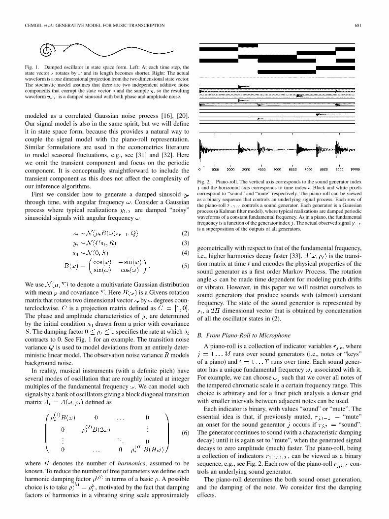
Fig. 1. Damped oscillator in state space form. Left: At each time step, thestate vector s rotates by ! and its length becomes shorter. Right: The actualwaveform is a one dimensional projection from the two dimensional state vector.The stochastic model assumes that there are two independent additive noisecomponents that corrupt the state vector s and the sample y, so the resultingwaveform y is a damped sinusoid with both phase and amplitude noise.
modeled as a correlated Gaussian noise process [16], [20].Our signal model is also in the same spirit, but we will defineit in state space form, because this provides a natural way tocouple the signal model with the piano-roll representation.Similar formulations are used in the econometrics literatureto model seasonal fluctuations, e.g., see [31] and [32]. Herewe omit the transient component and focus on the periodiccomponent. It is conceptually straightforward to include thetransient component as this does not affect the complexity ofour inference algorithms.
First we consider how to generate a damped sinusoidthrough time, with angular frequency . Consider a Gaussianprocess where typical realizations are damped “noisy”sinusoidal signals with angular frequency
(2)
(3)
(4)
(5)
We use to denote a multivariate Gaussian distributionwith mean and covariance . Here is a Givens rotationmatrix that rotates two dimensional vector by degrees coun-terclockwise. is a projection matrix defined as .The phase and amplitude characteristics of are determinedby the initial condition drawn from a prior with covariance
. The damping factor specifies the rate at whichcontracts to 0. See Fig. 1 for an example. The transition noisevariance is used to model deviations from an entirely deter-ministic linear model. The observation noise variance modelsbackground noise.
In reality, musical instruments (with a definite pitch) haveseveral modes of oscillation that are roughly located at integermultiples of the fundamental frequency . We can model suchsignals by a bank of oscillators giving a block diagonal transitionmatrix defined as
......
. . .(6)
where denotes the number of harmonics, assumed to beknown. To reduce the number of free parameters we define eachharmonic damping factor in terms of a basic . A possiblechoice is to take , motivated by the fact that dampingfactors of harmonics in a vibrating string scale approximately
Fig. 2. Piano-roll. The vertical axis corresponds to the sound generator indexj and the horizontal axis corresponds to time index t. Black and white pixelscorrespond to “sound” and “mute” respectively. The piano-roll can be viewedas a binary sequence that controls an underlying signal process. Each row ofthe piano-roll r controls a sound generator. Each generator is a Gaussianprocess (a Kalman filter model), where typical realizations are damped periodicwaveforms of a constant fundamental frequency. As in a piano, the fundamentalfrequency is a function of the generator index j. The actual observed signal yis a superposition of the outputs of all generators.
geometrically with respect to that of the fundamental frequency,i.e., higher harmonics decay faster [33]. is the transi-tion matrix at time and encodes the physical properties of thesound generator as a first order Markov Process. The rotationangle can be made time dependent for modeling pitch driftsor vibrato. However, in this paper we will restrict ourselves tosound generators that produce sounds with (almost) constantfrequency. The state of the sound generator is represented by
, a dimensional vector that is obtained by concatenationof all the oscillator states in (2).
B. From Piano-Roll to Microphone
A piano-roll is a collection of indicator variables , whereruns over sound generators (i.e., notes or “keys”
of a piano) and runs over time. Each sound gener-ator has a unique fundamental frequency associated with it.For example, we can choose such that we cover all notes ofthe tempered chromatic scale in a certain frequency range. Thischoice is arbitrary and for a finer pitch analysis a denser gridwith smaller intervals between adjacent notes can be used.
Each indicator is binary, with values “sound” or “mute”. Theessential idea is that, if previously muted, “mute”an onset for the sound generator occurs if “sound”.The generator continues to sound (with a characteristic dampingdecay) until it is again set to “mute”, when the generated signaldecays to zero amplitude (much) faster. The piano-roll, beinga collection of indicators , can be viewed as a binarysequence, e.g., see Fig. 2. Each row of the piano-roll con-trols an underlying sound generator.
The piano-roll determines the both sound onset generation,and the damping of the note. We consider first the dampingeffects.
682 IEEE TRANSACTIONS ON AUDIO, SPEECH, AND LANGUAGE PROCESSING, VOL. 14, NO. 2, MARCH 2006
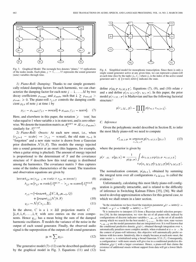
Fig. 3. Graphical Model. The rectangle box denotes “plates,” M replicationsof the nodes inside. Each plate, j = 1; . . . ;M represents the sound generator(note) variables through time.
1) Piano-Roll: Damping: Thanks to our simple geometri-cally related damping factors for each harmonic, we can char-acterize the damping factor for each note by twodecay coefficients and such that
. The piano-roll controls the damping coeffi-cient of note at time by
(7)
Here, and elsewhere in this paper, the notation hasvalue equal to 1 when variable is in state text, and is zero other-wise. We denote the transition matrix as ;similarly for .
2) Piano-Roll: Onsets: At each new onset, i.e., when, the old state is
“forgotten” and a new state vector is drawn from a Gaussianprior distribution . This models the energy injectedinto a sound generator at an onset (this happens, for example,when a guitar string is plucked). The amount of energy injectedis proportional to the determinant of and the covariancestructure of describes how this total energy is distributedamong the harmonics. The covariance matrix thus capturessome of the timbre characteristics of the sound. The transitionand observation equations are given by
(8)
(9)
(10)
(11)
In the above, is a projection matrixwith zero entries on the even compo-
nents. Hence has a mean being the sum of the dampedharmonic oscillators. models the variance of the noise in theoutput of each sound generator. Finally, the observed audiosignal is the superposition of the outputs of all sound generators
(12)
The generative model (7)–(12) can be described qualitativelyby the graphical model in Fig. 3. Equations (11) and (12)
Fig. 4. Simplified model for monophonic transcription. Since there is only asingle sound generator active at any given time, we can represent a piano-rollat each time slice by the tuple (j ; r ) where j is the index of the active soundgenerator and r 2 fsound;muteg indicates the state.
define . Equations (7), (9), and (10) relateand and define . In this paper, the priormodel is Markovian and has the following factorialstructure:1
C. Inference
Given the polyphonic model described in Section II, to inferthe most likely piano-roll we need to compute
(13)
where the posterior is given by
The normalization constant, , obtained by summingthe integral term over all configurations is called theevidence.2
Unfortunately, calculating this most likely piano-roll config-uration is generally intractable, and is related to the difficultyof inference in Switching Kalman Filters [35], [36]. We shallneed to develop approximation schemes for this general case, towhich we shall return in a later section.
1In the simulations we have fixed the transition parameter p(r = mutejr =sound) = p(r = soundjr = mute) = 10
2It is instructive to interpret (13) from a Bayesian model selection perspec-tive [34]. In this interpretation, we view the set of all piano-rolls, indexed byconfigurations of discrete indicator variables r , as the set of all modelsamong which we search for the best model r . In this view, state vectorss are the model parameters that are integrated over. It is well known thatthe conditional predictive density p(yjr), obtained through integration over s,automatically penalizes more complex models, when evaluated at y = y . Inthe context of piano-roll inference, this objective will automatically prefer so-lutions with less notes. Intuitively, this is simply because at each note onset, thestate vector s is reinitialized using a broad Gaussian N (0; S). Consequently,a configuration r with more onsets will give rise to a conditional predictive dis-tribution p(yjr) with a larger covariance. Hence, a piano-roll that claims theexistence of additional onsets without support from data will get a lower likeli-hood.
CEMGIL et al.: GENERATIVE MODEL FOR MUSIC TRANSCRIPTION 683
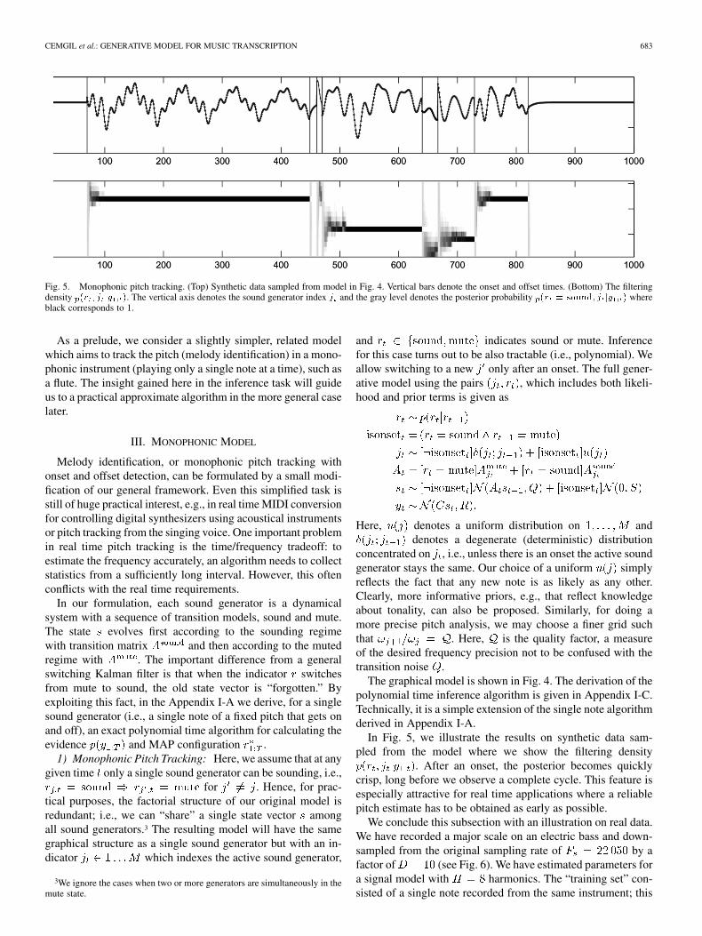
Fig. 5. Monophonic pitch tracking. (Top) Synthetic data sampled from model in Fig. 4. Vertical bars denote the onset and offset times. (Bottom) The filteringdensity p(r ; j jy ). The vertical axis denotes the sound generator index j and the gray level denotes the posterior probability p(r = sound; j jy ) whereblack corresponds to 1.
As a prelude, we consider a slightly simpler, related modelwhich aims to track the pitch (melody identification) in a mono-phonic instrument (playing only a single note at a time), such asa flute. The insight gained here in the inference task will guideus to a practical approximate algorithm in the more general caselater.
III. MONOPHONIC MODEL
Melody identification, or monophonic pitch tracking withonset and offset detection, can be formulated by a small modi-fication of our general framework. Even this simplified task isstill of huge practical interest, e.g., in real time MIDI conversionfor controlling digital synthesizers using acoustical instrumentsor pitch tracking from the singing voice. One important problemin real time pitch tracking is the time/frequency tradeoff: toestimate the frequency accurately, an algorithm needs to collectstatistics from a sufficiently long interval. However, this oftenconflicts with the real time requirements.
In our formulation, each sound generator is a dynamicalsystem with a sequence of transition models, sound and mute.The state evolves first according to the sounding regimewith transition matrix and then according to the mutedregime with . The important difference from a generalswitching Kalman filter is that when the indicator switchesfrom mute to sound, the old state vector is “forgotten.” Byexploiting this fact, in the Appendix I-A we derive, for a singlesound generator (i.e., a single note of a fixed pitch that gets onand off), an exact polynomial time algorithm for calculating theevidence and MAP configuration .
1) Monophonic Pitch Tracking: Here, we assume that at anygiven time only a single sound generator can be sounding, i.e.,
for . Hence, for prac-tical purposes, the factorial structure of our original model isredundant; i.e., we can “share” a single state vector amongall sound generators.3 The resulting model will have the samegraphical structure as a single sound generator but with an in-dicator which indexes the active sound generator,
3We ignore the cases when two or more generators are simultaneously in themute state.
and indicates sound or mute. Inferencefor this case turns out to be also tractable (i.e., polynomial). Weallow switching to a new only after an onset. The full gener-ative model using the pairs , which includes both likeli-hood and prior terms is given as
Here, denotes a uniform distribution on anddenotes a degenerate (deterministic) distribution
concentrated on , i.e., unless there is an onset the active soundgenerator stays the same. Our choice of a uniform simplyreflects the fact that any new note is as likely as any other.Clearly, more informative priors, e.g., that reflect knowledgeabout tonality, can also be proposed. Similarly, for doing amore precise pitch analysis, we may choose a finer grid suchthat . Here, is the quality factor, a measureof the desired frequency precision not to be confused with thetransition noise .
The graphical model is shown in Fig. 4. The derivation of thepolynomial time inference algorithm is given in Appendix I-C.Technically, it is a simple extension of the single note algorithmderived in Appendix I-A.
In Fig. 5, we illustrate the results on synthetic data sam-pled from the model where we show the filtering density
. After an onset, the posterior becomes quicklycrisp, long before we observe a complete cycle. This feature isespecially attractive for real time applications where a reliablepitch estimate has to be obtained as early as possible.
We conclude this subsection with an illustration on real data.We have recorded a major scale on an electric bass and down-sampled from the original sampling rate of by afactor of (see Fig. 6). We have estimated parameters fora signal model with harmonics. The “training set” con-sisted of a single note recorded from the same instrument; this
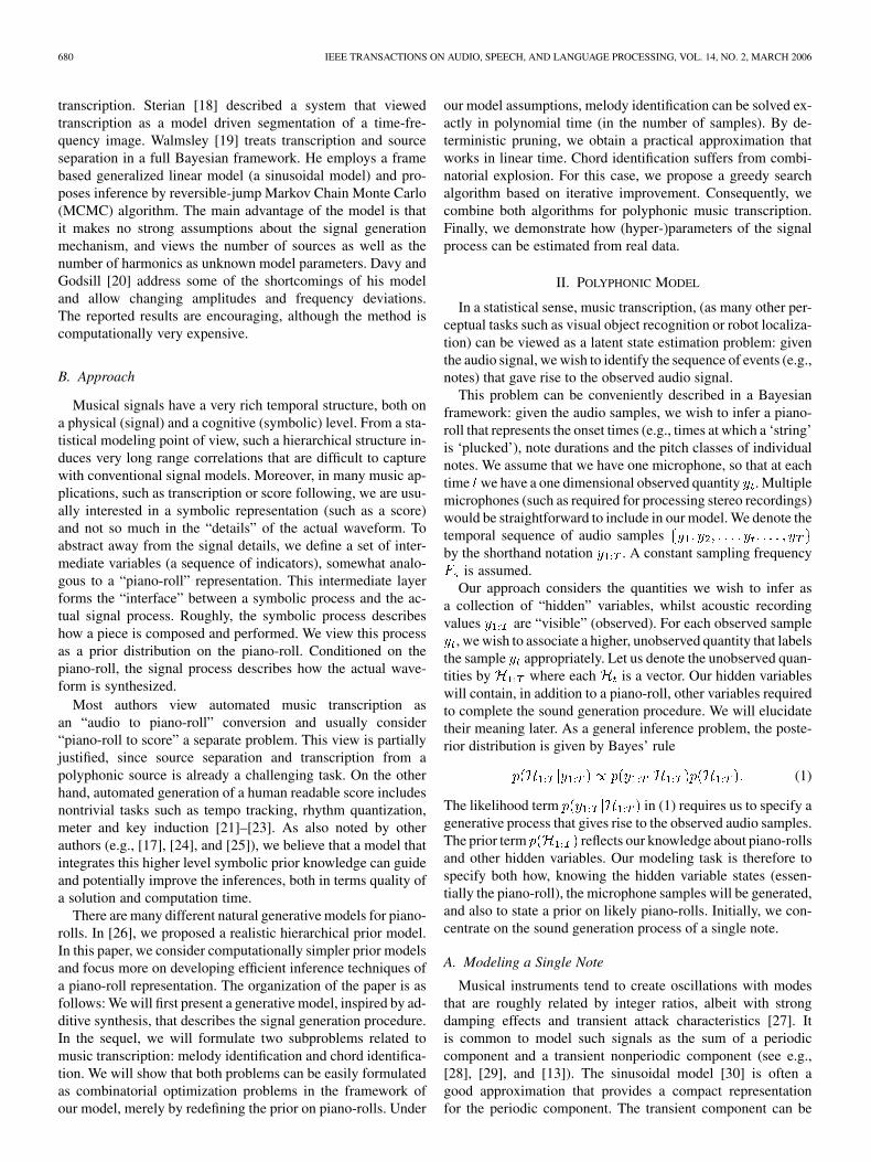
684 IEEE TRANSACTIONS ON AUDIO, SPEECH, AND LANGUAGE PROCESSING, VOL. 14, NO. 2, MARCH 2006
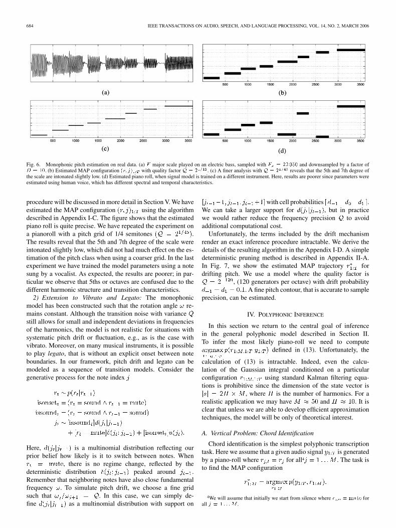
Fig. 6. Monophonic pitch estimation on real data. (a) F major scale played on an electric bass, sampled with F = 22050 and downsampled by a factor ofD = 10. (b) Estimated MAP configuration (r; j) with quality factor Q = 2 . (c) A finer analysis with Q = 2 reveals that the 5th and 7th degree ofthe scale are intonated slightly low. (d) Estimated piano roll, when signal model is trained on a different instrument. Here, results are poorer since parameters wereestimated using human voice, which has different spectral and temporal characteristics.
procedure will be discussed in more detail in Section V. We haveestimated the MAP configuration using the algorithmdescribed in Appendix I-C. The figure shows that the estimatedpiano roll is quite precise. We have repeated the experiment ona pianoroll with a pitch grid of 1/4 semitones .The results reveal that the 5th and 7th degree of the scale wereintonated slightly low, which did not had much effect on the es-timation of the pitch class when using a coarser grid. In the lastexperiment we have trained the model parameters using a notesung by a vocalist. As expected, the results are poorer; in par-ticular we observe that 5ths or octaves are confused due to thedifferent harmonic structure and transition characteristics.
2) Extension to Vibrato and Legato: The monophonicmodel has been constructed such that the rotation angle re-mains constant. Although the transition noise with variancestill allows for small and independent deviations in frequenciesof the harmonics, the model is not realistic for situations withsystematic pitch drift or fluctuation, e.g., as is the case withvibrato. Moreover, on many musical instruments, it is possibleto play legato, that is without an explicit onset between noteboundaries. In our framework, pitch drift and legato can bemodeled as a sequence of transition models. Consider thegenerative process for the note index
Here, is a multinomial distribution reflecting ourprior belief how likely is it to switch between notes. When
, there is no regime change, reflected by thedeterministic distribution peaked around .Remember that neighboring notes have also close fundamentalfrequency . To simulate pitch drift, we choose a fine gridsuch that . In this case, we can simply de-fine as a multinomial distribution with support on
with cell probabilities .We can take a larger support for , but in practicewe would rather reduce the frequency precision to avoidadditional computational cost.
Unfortunately, the terms included by the drift mechanismrender an exact inference procedure intractable. We derive thedetails of the resulting algorithm in the Appendix I-D. A simpledeterministic pruning method is described in Appendix II-A.In Fig. 7, we show the estimated MAP trajectory fordrifting pitch. We use a model where the quality factor is
, (120 generators per octave) with drift probability. A fine pitch contour, that is accurate to sample
precision, can be estimated.
IV. POLYPHONIC INFERENCE
In this section we return to the central goal of inferencein the general polyphonic model described in Section II.To infer the most likely piano-roll we need to compute
defined in (13). Unfortunately, the
calculation of (13) is intractable. Indeed, even the calcu-lation of the Gaussian integral conditioned on a particularconfiguration using standard Kalman filtering equa-tions is prohibitive since the dimension of the state vector is
, where is the number of harmonics. For arealistic application we may have and . It isclear that unless we are able to develop efficient approximationtechniques, the model will be only of theoretical interest.
A. Vertical Problem: Chord Identification
Chord identification is the simplest polyphonic transcriptiontask. Here we assume that a given audio signal is generatedby a piano-roll where for all4 . The task isto find the MAP configuration
4We will assume that initially we start from silence where r = mute forall j = 1 . . .M .
CEMGIL et al.: GENERATIVE MODEL FOR MUSIC TRANSCRIPTION 685
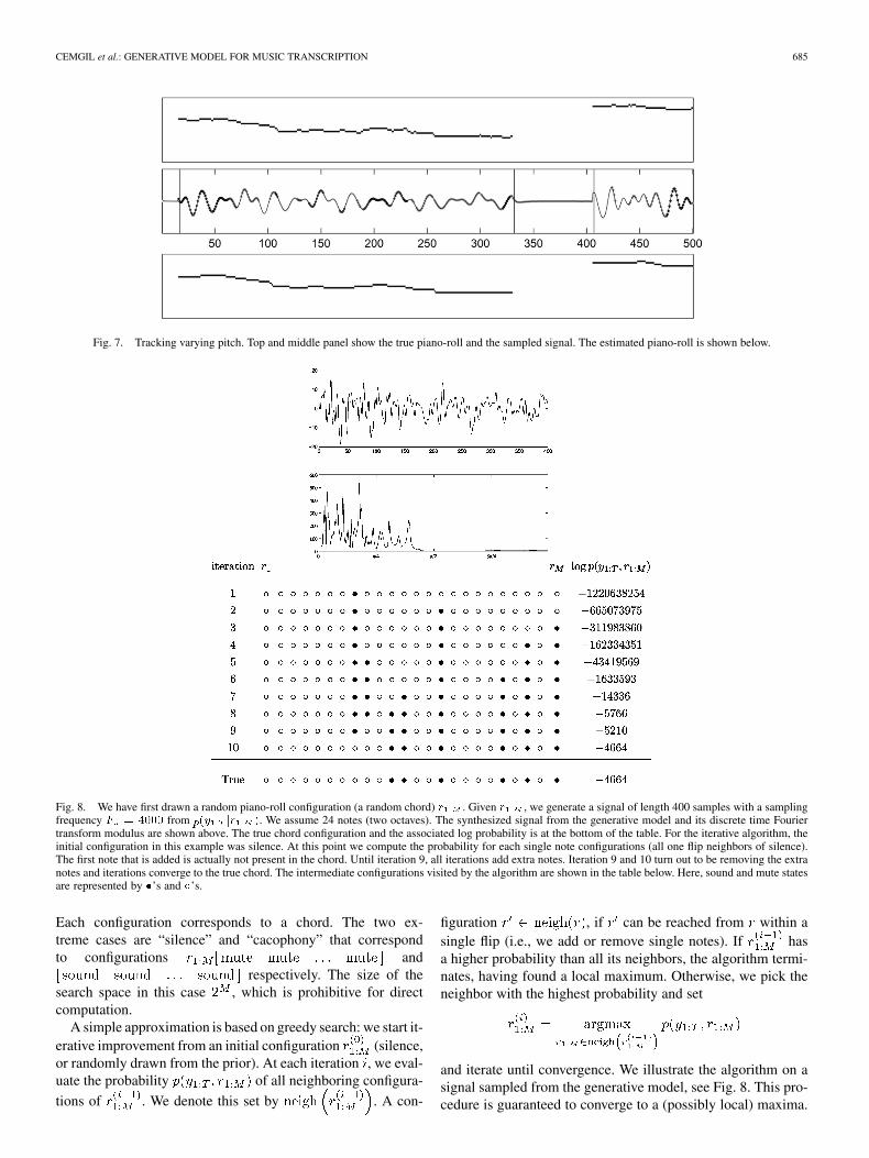
Fig. 7. Tracking varying pitch. Top and middle panel show the true piano-roll and the sampled signal. The estimated piano-roll is shown below.
Fig. 8. We have first drawn a random piano-roll configuration (a random chord) r . Given r , we generate a signal of length 400 samples with a samplingfrequency F = 4000 from p(y jr ). We assume 24 notes (two octaves). The synthesized signal from the generative model and its discrete time Fouriertransform modulus are shown above. The true chord configuration and the associated log probability is at the bottom of the table. For the iterative algorithm, theinitial configuration in this example was silence. At this point we compute the probability for each single note configurations (all one flip neighbors of silence).The first note that is added is actually not present in the chord. Until iteration 9, all iterations add extra notes. Iteration 9 and 10 turn out to be removing the extranotes and iterations converge to the true chord. The intermediate configurations visited by the algorithm are shown in the table below. Here, sound and mute statesare represented by �’s and �’s.
Each configuration corresponds to a chord. The two ex-treme cases are “silence” and “cacophony” that correspondto configurations and
respectively. The size of thesearch space in this case , which is prohibitive for directcomputation.
A simple approximation is based on greedy search: we start it-erative improvement from an initial configuration (silence,or randomly drawn from the prior). At each iteration , we eval-uate the probability of all neighboring configura-
tions of . We denote this set by . A con-
figuration , if can be reached from within asingle flip (i.e., we add or remove single notes). If hasa higher probability than all its neighbors, the algorithm termi-nates, having found a local maximum. Otherwise, we pick theneighbor with the highest probability and set
and iterate until convergence. We illustrate the algorithm on asignal sampled from the generative model, see Fig. 8. This pro-cedure is guaranteed to converge to a (possibly local) maxima.
686 IEEE TRANSACTIONS ON AUDIO, SPEECH, AND LANGUAGE PROCESSING, VOL. 14, NO. 2, MARCH 2006
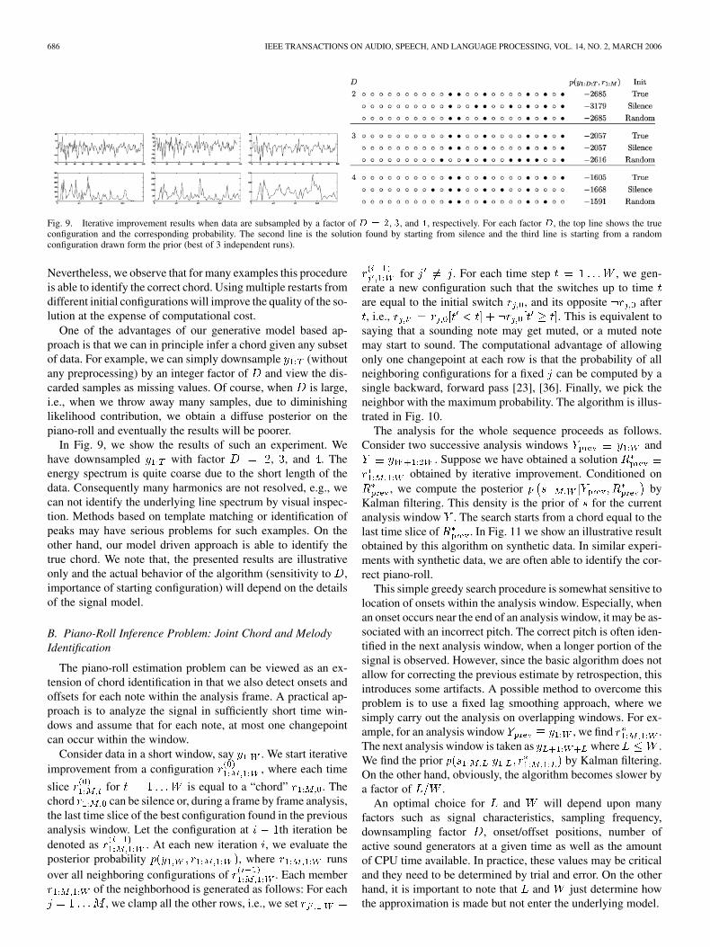
Fig. 9. Iterative improvement results when data are subsampled by a factor of D = 2, 3, and 4, respectively. For each factor D, the top line shows the trueconfiguration and the corresponding probability. The second line is the solution found by starting from silence and the third line is starting from a randomconfiguration drawn form the prior (best of 3 independent runs).
Nevertheless, we observe that for many examples this procedureis able to identify the correct chord. Using multiple restarts fromdifferent initial configurations will improve the quality of the so-lution at the expense of computational cost.
One of the advantages of our generative model based ap-proach is that we can in principle infer a chord given any subsetof data. For example, we can simply downsample (withoutany preprocessing) by an integer factor of and view the dis-carded samples as missing values. Of course, when is large,i.e., when we throw away many samples, due to diminishinglikelihood contribution, we obtain a diffuse posterior on thepiano-roll and eventually the results will be poorer.
In Fig. 9, we show the results of such an experiment. Wehave downsampled with factor , , and . Theenergy spectrum is quite coarse due to the short length of thedata. Consequently many harmonics are not resolved, e.g., wecan not identify the underlying line spectrum by visual inspec-tion. Methods based on template matching or identification ofpeaks may have serious problems for such examples. On theother hand, our model driven approach is able to identify thetrue chord. We note that, the presented results are illustrativeonly and the actual behavior of the algorithm (sensitivity to ,importance of starting configuration) will depend on the detailsof the signal model.
B. Piano-Roll Inference Problem: Joint Chord and MelodyIdentification
The piano-roll estimation problem can be viewed as an ex-tension of chord identification in that we also detect onsets andoffsets for each note within the analysis frame. A practical ap-proach is to analyze the signal in sufficiently short time win-dows and assume that for each note, at most one changepointcan occur within the window.
Consider data in a short window, say . We start iterativeimprovement from a configuration , where each time
slice for is equal to a “chord” . Thechord can be silence or, during a frame by frame analysis,the last time slice of the best configuration found in the previousanalysis window. Let the configuration at th iteration bedenoted as . At each new iteration , we evaluate theposterior probability , where runsover all neighboring configurations of . Each member
of the neighborhood is generated as follows: For each, we clamp all the other rows, i.e., we set
for . For each time step , we gen-erate a new configuration such that the switches up to timeare equal to the initial switch , and its opposite after, i.e., . This is equivalent to
saying that a sounding note may get muted, or a muted notemay start to sound. The computational advantage of allowingonly one changepoint at each row is that the probability of allneighboring configurations for a fixed can be computed by asingle backward, forward pass [23], [36]. Finally, we pick theneighbor with the maximum probability. The algorithm is illus-trated in Fig. 10.
The analysis for the whole sequence proceeds as follows.Consider two successive analysis windows and
. Suppose we have obtained a solutionobtained by iterative improvement. Conditioned on
, we compute the posterior byKalman filtering. This density is the prior of for the currentanalysis window . The search starts from a chord equal to thelast time slice of . In Fig. 11 we show an illustrative resultobtained by this algorithm on synthetic data. In similar experi-ments with synthetic data, we are often able to identify the cor-rect piano-roll.
This simple greedy search procedure is somewhat sensitive tolocation of onsets within the analysis window. Especially, whenan onset occurs near the end of an analysis window, it may be as-sociated with an incorrect pitch. The correct pitch is often iden-tified in the next analysis window, when a longer portion of thesignal is observed. However, since the basic algorithm does notallow for correcting the previous estimate by retrospection, thisintroduces some artifacts. A possible method to overcome thisproblem is to use a fixed lag smoothing approach, where wesimply carry out the analysis on overlapping windows. For ex-ample, for an analysis window , we find .The next analysis window is taken as where .We find the prior by Kalman filtering.On the other hand, obviously, the algorithm becomes slower bya factor of .
An optimal choice for and will depend upon manyfactors such as signal characteristics, sampling frequency,downsampling factor , onset/offset positions, number ofactive sound generators at a given time as well as the amountof CPU time available. In practice, these values may be criticaland they need to be determined by trial and error. On the otherhand, it is important to note that and just determine howthe approximation is made but not enter the underlying model.
CEMGIL et al.: GENERATIVE MODEL FOR MUSIC TRANSCRIPTION 687
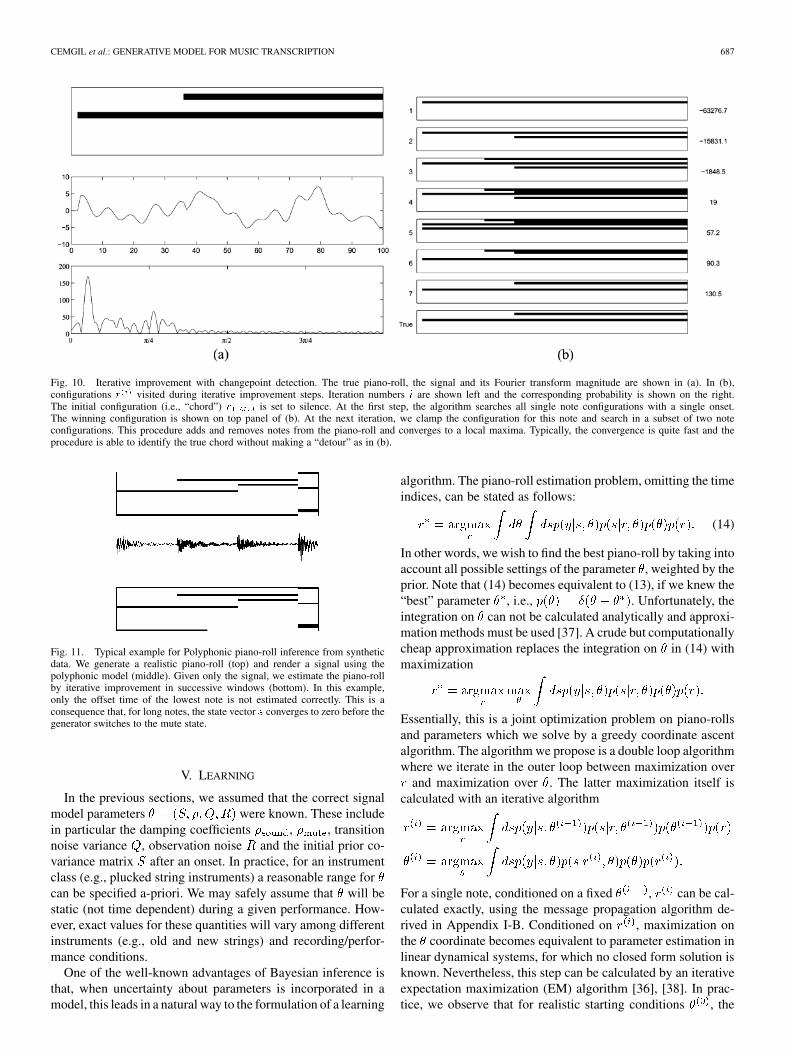
Fig. 10. Iterative improvement with changepoint detection. The true piano-roll, the signal and its Fourier transform magnitude are shown in (a). In (b),configurations r visited during iterative improvement steps. Iteration numbers i are shown left and the corresponding probability is shown on the right.The initial configuration (i.e., “chord”) r is set to silence. At the first step, the algorithm searches all single note configurations with a single onset.The winning configuration is shown on top panel of (b). At the next iteration, we clamp the configuration for this note and search in a subset of two noteconfigurations. This procedure adds and removes notes from the piano-roll and converges to a local maxima. Typically, the convergence is quite fast and theprocedure is able to identify the true chord without making a “detour” as in (b).
Fig. 11. Typical example for Polyphonic piano-roll inference from syntheticdata. We generate a realistic piano-roll (top) and render a signal using thepolyphonic model (middle). Given only the signal, we estimate the piano-rollby iterative improvement in successive windows (bottom). In this example,only the offset time of the lowest note is not estimated correctly. This is aconsequence that, for long notes, the state vector s converges to zero before thegenerator switches to the mute state.
V. LEARNING
In the previous sections, we assumed that the correct signalmodel parameters were known. These includein particular the damping coefficients , , transitionnoise variance , observation noise and the initial prior co-variance matrix after an onset. In practice, for an instrumentclass (e.g., plucked string instruments) a reasonable range forcan be specified a-priori. We may safely assume that will bestatic (not time dependent) during a given performance. How-ever, exact values for these quantities will vary among differentinstruments (e.g., old and new strings) and recording/perfor-mance conditions.
One of the well-known advantages of Bayesian inference isthat, when uncertainty about parameters is incorporated in amodel, this leads in a natural way to the formulation of a learning
algorithm. The piano-roll estimation problem, omitting the timeindices, can be stated as follows:
(14)
In other words, we wish to find the best piano-roll by taking intoaccount all possible settings of the parameter , weighted by theprior. Note that (14) becomes equivalent to (13), if we knew the“best” parameter , i.e., . Unfortunately, theintegration on can not be calculated analytically and approxi-mation methods must be used [37]. A crude but computationallycheap approximation replaces the integration on in (14) withmaximization
Essentially, this is a joint optimization problem on piano-rollsand parameters which we solve by a greedy coordinate ascentalgorithm. The algorithm we propose is a double loop algorithmwhere we iterate in the outer loop between maximization over
and maximization over . The latter maximization itself iscalculated with an iterative algorithm
For a single note, conditioned on a fixed , can be cal-culated exactly, using the message propagation algorithm de-rived in Appendix I-B. Conditioned on , maximization onthe coordinate becomes equivalent to parameter estimation inlinear dynamical systems, for which no closed form solution isknown. Nevertheless, this step can be calculated by an iterativeexpectation maximization (EM) algorithm [36], [38]. In prac-tice, we observe that for realistic starting conditions , the
688 IEEE TRANSACTIONS ON AUDIO, SPEECH, AND LANGUAGE PROCESSING, VOL. 14, NO. 2, MARCH 2006
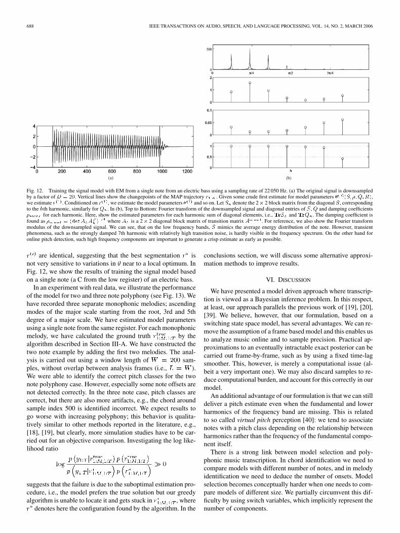
Fig. 12. Training the signal model with EM from a single note from an electric bass using a sampling rate of 22 050 Hz. (a) The original signal is downsampledby a factor ofD = 20. Vertical lines show the changepoints of the MAP trajectory r . Given some crude first estimate for model parameters � (S; �;Q;R),we estimate r . Conditioned on r , we estimate the model parameters � and so on. Let S denote the 2� 2 block matrix from the diagonal S, correspondingto the hth harmonic, similarly for Q . In (b), Top to Bottom: Fourier transform of the downsampled signal and diagonal entries of S, Q and damping coefficients� for each harmonic. Here, show the estimated parameters for each harmonic sum of diagonal elements, i.e., TrS and TrQ . The damping coefficient isfound as � = (detA A ) where A is a 2� 2 diagonal block matrix of transition matrix A . For reference, we also show the Fourier transformmodulus of the downsampled signal. We can see, that on the low frequency bands, S mimics the average energy distribution of the note. However, transientphenomena, such as the strongly damped 7th harmonic with relatively high transition noise, is hardly visible in the frequency spectrum. On the other hand foronline pitch detection, such high frequency components are important to generate a crisp estimate as early as possible.
are identical, suggesting that the best segmentation isnot very sensitive to variations in near to a local optimum. InFig. 12, we show the results of training the signal model basedon a single note (a C from the low register) of an electric bass.
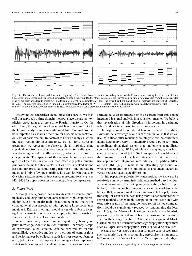
In an experiment with real data, we illustrate the performanceof the model for two and three note polyphony (see Fig. 13). Wehave recorded three separate monophonic melodies; ascendingmodes of the major scale starting from the root, 3rd and 5thdegree of a major scale. We have estimated model parametersusing a single note from the same register. For each monophonicmelody, we have calculated the ground truth by thealgorithm described in Section III-A. We have constructed thetwo note example by adding the first two melodies. The anal-ysis is carried out using a window length of sam-ples, without overlap between analysis frames (i.e., ).We were able to identify the correct pitch classes for the twonote polyphony case. However, especially some note offsets arenot detected correctly. In the three note case, pitch classes arecorrect, but there are also more artifacts, e.g., the chord aroundsample index 500 is identified incorrect. We expect results togo worse with increasing polyphony; this behavior is qualita-tively similar to other methods reported in the literature, e.g.,[18], [19], but clearly, more simulation studies have to be car-ried out for an objective comparison. Investigating the log like-lihood ratio
suggests that the failure is due to the suboptimal estimation pro-cedure, i.e., the model prefers the true solution but our greedyalgorithm is unable to locate it and gets stuck in , where
denotes here the configuration found by the algorithm. In the
conclusions section, we will discuss some alternative approxi-mation methods to improve results.
VI. DISCUSSION
We have presented a model driven approach where transcrip-tion is viewed as a Bayesian inference problem. In this respect,at least, our approach parallels the previous work of [19], [20],[39]. We believe, however, that our formulation, based on aswitching state space model, has several advantages. We can re-move the assumption of a frame based model and this enables usto analyze music online and to sample precision. Practical ap-proximations to an eventually intractable exact posterior can becarried out frame-by-frame, such as by using a fixed time-lagsmoother. This, however, is merely a computational issue (al-beit a very important one). We may also discard samples to re-duce computational burden, and account for this correctly in ourmodel.
An additional advantage of our formulation is that we can stilldeliver a pitch estimate even when the fundamental and lowerharmonics of the frequency band are missing. This is relatedto so called virtual pitch perception [40]: we tend to associatenotes with a pitch class depending on the relationship betweenharmonics rather than the frequency of the fundamental compo-nent itself.
There is a strong link between model selection and poly-phonic music transcription. In chord identification we need tocompare models with different number of notes, and in melodyidentification we need to deduce the number of onsets. Modelselection becomes conceptually harder when one needs to com-pare models of different size. We partially circumvent this dif-ficulty by using switch variables, which implicitly represent thenumber of components.
CEMGIL et al.: GENERATIVE MODEL FOR MUSIC TRANSCRIPTION 689
Fig. 13. Experiment with two and three note polyphony. Three monophonic melodies (ascending modes of the F major scale starting from the root, 3rd and5th degree) are recorded and transcribed separately to obtain the ground truth. Model parameters are learned using a single note recorded from the same register.Finally, melodies are added to create two- and three-note polyphonic examples. (a) (Top) The ground truth estimated when all melodies are transcribed separately.(Middle) The superposition of first two melodies downsampled by a factor ofD = 10. (Bottom) Piano-roll estimated with an analysis window of sizeW = 200
samples, without overlap between analysis frames. (b) Result for the same experiment with three notes polyphony.
Following the established signal processing jargon, we maycall our approach a time-domain method, since we are not ex-plicitly calculating a discrete-time Fourier transform. On theother hand, the signal model presented here has close links tothe Fourier analysis and sinusoidal modeling. Our analysis canbe interpreted as a search procedure for a sparse representationon a set of basis vectors. In contrast to Fourier analysis, wherethe basis vectors are sinusoids (e.g., see [41] for a Bayesiantreatment), we represent the observed signal implicitly usingsignals drawn from a stochastic process which typically gener-ates decaying periodic oscillations (e.g., notes) with occasionalchangepoints. The sparsity of this representation is a conse-quence of the onset mechanism, that effectively puts a mixtureprior over the hidden state vector . This prior is peaked aroundzero and has broad tails, indicating that most of the sources aremuted and only a few are sounding. It is well known that suchGaussian mixture priors induce sparse representations, e.g., see[42], [43] for applications in the context of source separation.
A. Future Work
Although our approach has many desirable features (auto-matically deducing number of correct notes, high temporal res-olution e.t.c.), one of the main disadvantage of our method iscomputational cost associated with updating large covariancematrices in Kalman filtering. It would be very desirable to inves-tigate approximation schemas that employ fast transformationssuch as the FFT to accelerate computations.
When transcribing music, human experts rely heavily onprior knowledge about the musical structure—harmony, tempoor expression. Such structure can be captured by trainingprobabilistic generative models on a corpus of compositionsand performances by collecting statistics over selected features(e.g., [44]). One of the important advantages of our approachis that such prior knowledge about the musical structure can be
formulated as an informative prior on a piano-roll; thus can beintegrated in signal analysis in a consistent manner. We believethat investigation of this direction is important in designingrobust and practical music transcription systems.
Our signal model considered here is inspired by additivesynthesis. An advantage of our linear formulation is that we canuse the Kalman filter recursions to integrate out the continuouslatent state analytically. An alternative would be to formulatea nonlinear dynamical system that implements a nonlinearsynthesis model (e.g., FM synthesis, waveshaping synthesis, oreven a physical model [45]). Such an approach would reducethe dimensionality of the latent state space but force us touse approximate integration methods such as particle filtersor EKF/UKF [46]. It remains an interesting open questionwhether, in practice, one should trade-off analytical tractabilityversus reduced latent state dimension.
In this paper, for polyphonic transcription, we have used arelatively simple deterministic inference method based on iter-ative improvement. The basic greedy algorithm, whilst still po-tentially useful in practice, may get stuck in poor solutions. Webelieve that, using our model as a framework, better polyphonictranscriptions can be achieved using more elaborate inference orsearch methods. For example, computation time associated withexhaustive search of the neighborhood for all visited configua-tions could be significantly reduced by randomizing the localsearch (e.g., by Metropolis-Hastings moves5) or use heuristicproposal distributions derived from easy-to-compute featuressuch as the energy spectrum. Alternatively, sequential MonteCarlo methods or deterministic message propagation algorithmssuch as Expectation propagation (EP) [47] could be also used.
We have not yet tested our model for more general scenarios,such as music fragments containing percussive instruments orbell sounds with inharmonic spectra. Our simple periodic signal
5This improvement is suggested by one of the anonymous reviewers.
690 IEEE TRANSACTIONS ON AUDIO, SPEECH, AND LANGUAGE PROCESSING, VOL. 14, NO. 2, MARCH 2006
model would be clearly inadequate for such a scenario. On theother hand, we stress the fact that the framework presented hereis not limited to the analysis of signals with harmonic spectra,and in principle applicable to any family of signals that can berepresented by a switching state space model. This is already alarge class since many real-world acoustic processes can be ap-proximated well with piecewise linear regimes. We can also for-mulate a joint estimation schema for unknown parameters as in(14) and integrate them out (e.g., see [20]). However, this is cur-rently a hard and computationally expensive task. If efficient andaccurate approximate integration methods can be developed, ourmodel will be applicable to mixtures of many different types ofacoustical signals and may be useful in more general auditoryscene analysis problems.
APPENDIX IDERIVATION OF MESSAGE PROPAGATION ALGORITHMS
In the appendix, we derive several exact message propaga-tion algorithms. Our derivation closely follows the standardderivation of recursive prediction and update equations for theKalman filter [48]. First we focus on a single sound generator. InAppendices I-A and B, we derive polynomial time algorithmsfor calculating the evidence and MAP configuration
respectively. The MAP config-
uration is useful for onset/offset detection. In the followingsection, we extend the onset/offset detection algorithms tomonophonic pitch tracking with constant frequency. We derivea polynomial time algorithm for this case in Appendix I-C.The case for varying fundamental frequency is derived in thefollowing Appendix I-D. In Appendix II we describe heuristicsto reduce the amount of computations.
A. Computation of the Evidence for a Single SoundGenerator by Forward Filtering
We assume a Markovian prior on the indicators , where. For convenience, we repeat the
generative model for a single sound generator by omitting thenote index
For simplicity, we will sometime use the labels 1 and 2 to de-note sound and mute respectively. We enumerate the transitionmodels as . We define the fil-tering potential as
We assume that is always observed, hence we use the term po-tential to indicate the fact that is not normal-ized. The filtering potential is in general a conditional Gaussianmixture, i.e., a mixture of Gaussians for each configuration of
. We will highlight this data structure by using the fol-lowing notation
where each forare also Gaussian mixture potentials. We will denote the
conditional normalization constants as
Consequently the evidence is given by
We also define the predictive density
In general, for switching Kalman filters, calculating exactposterior features, such as the evidence , is nottractable. This is a consequence of the fact that the numberof mixture components to required to represent the exact fil-tering density grows exponentially with time step (i.e.,one Gaussian for each of the exponentially many configurations
). Luckily, for the model we are considering here, the growthis polynomial in only. See also [49].
To see this, suppose we have the filtering density availableat time as . The transition models can be organizedalso in a table where th row and th column correspond to
Calculation of the predictive potential is straightforward.First, summation over yields
Integration over and multiplication by yieldsthe predictive potential
where we define
The potentials can be computed by applying the standardKalman prediction equations to each component of . Theupdated potential is given by . This quantity
CEMGIL et al.: GENERATIVE MODEL FOR MUSIC TRANSCRIPTION 691
can be computed by applying standard Kalman update equationsto each component of .
From the above derivation, it is clear that has only asingle Gaussian component. This has the consequence that thenumber of Gaussian components in increases only linearly(the first row-sum terms propagated through ). Thesecond row sum term is more costly; it increases at everytime slice by the number of components in . Since the sizeof grows linearly, the size of grows quadratically withtime .
B. Computation of Map Configuration
The MAP state is defined as
For finding the MAP state, we replace summations over bymaximization. One potential technical difficulty is that, unlike inthe case for evidence calculation, maximization and integrationdo not commute. Consider a conditional Gaussian potential
where are Gaussian potentials for each configuration of. We can compute the MAP configuration
where . We evaluate the normalization ofeach component (i.e., integrate over the continuous hidden vari-able first) and finally find the maximum of all normalizationconstants.
However, direct calculation of is not feasible becauseof exponential explosion in the number of distinct configura-tions. Fortunately, for our model, we can introduce a determin-istic pruning schema that reduces the number of kernels to apolynomial order and meanwhile guarantees that we will nevereliminate the MAP configuration. This exact pruning methodhinges on the factorization of the posterior for the assignmentof variables , (mute to sound transition) thatbreaks the direct link between and
(15)
In this case
(16)
This equation shows that whenever we have an onset, we can cal-culate the maximum over the past and future configurations sep-arately. Put differently, provided that the MAP configuration hasthe form , the prefix
will be the solution for the reduced maxi-mization problem .
1) Forward Pass: Suppose we have a collection of Gaussianpotentials
with the property that the Gaussian kernel corresponding theprefix of the MAP state is a member of , i.e.,
s.t. . We alsodefine the subsets
We show how we find . The prediction is given by
The multiplication by and integration overyields the predictive potential , as shown in the equation atthe bottom of the page. By (16), we can replace the collection ofnumbers with the scalarwithout changing the optimum solution
The updated potential is given by . The anal-ysis of the number of kernels proceeds as in the previous section.
2) Decoding: During the forward pass, we tag eachGaussian component of with its past history of . The
692 IEEE TRANSACTIONS ON AUDIO, SPEECH, AND LANGUAGE PROCESSING, VOL. 14, NO. 2, MARCH 2006
MAP state can be found by a simple search in the collection ofpolynomially many numbers and reporting the associated tag
We finally conclude that the forward filtering and MAP (Viterbipath) estimation algorithms are essentially identical with sum-mation replaced by maximization and an additional tagging re-quired for decoding.
C. Inference for Monophonic Pitch Tracking
In this section we derive an exact message propagation algo-rithm for monophonic pitch tracking. Perhaps surprisingly, in-ference in this case turns out to be still tractable. Even though thesize of the configuration space is of size
, the space complexity of an exact algorithm re-mains quadratic in . First, we define a “mega” indicator node
where indicates the index of the ac-tive sound generator and indicates its state.The transition model is a large sparse transition tablewith probabilities
. . ....
. . ....
. . .. . .
(17)
where the transitions are orga-nized at the th row and th column whereand (17). The transition models
can be organizedsimilarly
. . ....
. . ....
. . .. . .
Here, denotes the transition model of theth sound generator when in state . The derivation for filtering
follows the same lines as the onset/offset detection model, withonly slightly more tedious indexing. Suppose we have the fil-tering density available at time as . We first calculatethe predictive potential. Summation over yields the rowsums
Integration over and multiplication by yieldsthe predictive potential . The components are given as
otherwise(18)
where we define
The potentials can be computed by applying the standardKalman prediction equations to each component of . Note thatthe forward messages have the same sparsity structure as theprior, i.e., when
is nonzero. The updated potential is given by. This quantity can be computed by applying stan-
dard Kalman update equations to each nonzero component of.
D. Monophonic Pitch Tracking With Varying FundamentalFrequency
We model pitch drift by a sequence of transition models. Wechoose a grid such that , where is close to one.Unfortunately, the subdiagonal terms introduced to the priortransition matrix
. . .. . .
. . .
(19)
render an exact algorithm exponential in . The recursive updateequations, starting with , are obtained by summing over
, integration over and multiplication by .The only difference is that the prediction (18) needs to bechanged to
where and are defined in (19). The reason for theexponential growth is the following: Remember that each
has as many components as an entire row sum of. Unlike the inference for piecewise
constant pitch estimation, now at some rows there are two ormore messages (e.g., and ) that dependon .
CEMGIL et al.: GENERATIVE MODEL FOR MUSIC TRANSCRIPTION 693
APPENDIX IICOMPUTATIONAL SIMPLIFICATIONS
A. Pruning
Exponential growth in message size renders an algorithm use-less in practice. Even in special cases, where the message sizeincreases only polynomially in , this growth is still prohibitivefor many applications. A cheaper approximate algorithm can beobtained by pruning the messages. To keep the size of messagesbounded, we limit the number of components to and storeonly components with the highest evidence. An alternative isdiscarding components of a message that contribute less than agiven fraction (e.g., 0.0001) to the total evidence. More sophis-ticated pruning methods with profound theoretical justification,such as resampling [23] or collapsation [50], are viable alterna-tives but these are computationally more expensive. In our simu-lations, we observe that using a simple pruning method with themaximum number of components per message set to ,we can obtain results very close to an exact algorithm.
B. Kalman Filtering in a Reduced Dimension
Kalman filtering with a large state dimension at typicalaudio sampling rates kHz may be prohibitive withgeneric hardware. This problem becomes more severe when thenumber of notes is large, (which is typically around 50–60),than even conditioned on a particular configuration , thecalculation of the filtering density is expensive. Hence, in animplementation, tricks of precomputing the covariance matricescan be considered [48] to further reduce the computationalburden.
Another important simplification is less obvious from thegraphical structure and is a consequence of the inherent asym-metry between the sound and mute states. Typically, when anote switches and stays for a short period in the mute state, i.e.,
for some period, the marginal posterior over thestate vector will converge quickly to a zero mean Gaussianwith a small covariance matrix regardless of observations .We exploit this property to save computations by clamping thehidden states for sequences of to zero for “mute”.This reduces the hidden state dimension, since typically, only afew sound generators will be in sound state.
REFERENCES
[1] A. Bregman, Auditory Scene Analysis. Cambridge, MA: MIT Press,1990.
[2] G. J. Brown and M. Cooke, “Computational auditory scene analysis,”Comput. Speech Lang., vol. 8, no. 2, pp. 297–336, 1994.
[3] M. Weintraub, “A theory and computational model of auditory monauralsound separation,” Ph.D. dissertation, Dept. Elect. Eng., Stanford Univ.,Stanford, CA, 1985.
[4] S. Roweis, “One microphone source separation,” in Neural InformationProcessing Systems, NIPS*2000, 2001.
[5] D. P. W. Ellis, “Prediction-driven computational auditory scene anal-ysis,” Ph.D. dissertation, Dept. Elect. Eng. Comput. Sci., Mass. Inst.Technol., Cambridge, MA, 1996.
[6] E. D. Scheirer, “Music-Listening Systems,” Ph.D. dissertation, Dept.Elect. Eng. Comput. Sci., Mass. Inst. Technol., Cambridge, MA,2000.
[7] G. Tzanetakis, “Manipulation, analysis and retrieval systems for audiosignals,” Ph.D. dissertation, Princeton Univ., Princeton, NJ, 2002.
[8] R. Rowe, Machine Musichanship. Cambridge, MA: MIT Press, 2001.
[9] M. Plumbley, S. Abdallah, J. P. Bello, M. Davies, G. Monti, and M.Sandler, “Automatic music transcription and audio source separation,”Cybern. Syst., vol. 33, no. 6, pp. 603–627, 2002.
[10] W. J. Hess, Pitch Determination of Speech Signal. New York:Springer, 1983.
[11] B. G. Quinn and E. J. Hannan, The Estimation and Tracking of Fre-quency. Cambridge, U.K.: Cambridge Univ. Press, 2001.
[12] R. A. Irizarry, “Local harmonic estimation in musical sound signals,” J.Amer. Statist. Assoc., 2001, to be published.
[13] , “Weighted estimation of harmonic components in a musical soundsignal,” J. Time Series Anal., vol. 23, 2002.
[14] K. L. Saul, D. D. Lee, C. L. Isbell, and Y. LeCun, “Real time voiceprocessing with audiovisual feedback: Toward autonomous agentswith perfect pitch,” in Neural Information Processing Systems,NIPS*2002 Vancouver, BC, Canada, 2002.
[15] B. Truong-Van, “A new approach to frequency analysis with amplifiedharmonics,” J. R. Statist. Soc. B, no. 52, pp. 203–222, 1990.
[16] L. Parra and U. Jain, “Approximate kalman filtering for the harmonicplus noise model,” in Proc. IEEE WASPAA, New Paltz, NY, 2001.
[17] K. Kashino, K. Nakadai, T. Kinoshita, and H. Tanaka, “Application ofBayesian probability network to music scene analysis,” in Proc. IJCAIWorkshop CASA, Montreal, QC, Canada, 1995, pp. 52–59.
[18] A. Sterian, “Model-based segmentation of time-frequency images formusical transcription,” Ph.D. dissertation, Univ. Michigan, Ann Arbor,1999.
[19] P. J. Walmsley, “Signal separation of musical instruments,” Ph.D. dis-sertation, Univ. Cambridge, Cambridge, U.K., 2000.
[20] M. Davy and S. J. Godsill, “Bayesian harmonic models for musicalsignal analysis,” Bayesian Statist. 7, 2003.
[21] C. Raphael, “A mixed graphical model for rhythmic parsing,” in Proc.17th Conf. Uncertainty Artif. Intell., 2001.
[22] D. Temperley, The Cognition of Basic Musical Structures. Cambridge,MA: MIT Press, 2001.
[23] A. T. Cemgil and H. J. Kappen, “Monte Carlo methods for tempotracking and rhythm quantization,” J. Artif. Intell. Res., vol. 18, pp.45–81, 2003.
[24] K. Martin, “Sound-Source Recognition,” Ph.D. dissertation, MIT, Cam-bridge, MA, 1999.
[25] A. Klapuri, T. Virtanen, and J.-M. Holm, “Robust multipitch estima-tion for the analysis and manipulation of polyphonic musical signals,”in Proc. COST-G6, Conf. Digital Audio Effects, 2000.
[26] A. T. Cemgil, H. J. Kappen, and D. Barber, “Generative model basedpolyphonic music transcription,” in Proc. IEEE WASPAA, New Paltz,NY, Oct. 2003.
[27] N. H. Fletcher and T. Rossing, The Physics of Musical Instru-ments. New York: Springer, 1998.
[28] X. Serra and J. O. Smith, “Spectral modeling synthesis: A sound anal-ysis/synthesis system based on deterministic plus stochastic decompo-sition,” Comput. Music J., vol. 14, no. 4, pp. 12–24, 1991.
[29] X. Rodet, “Musical sound signals analysis/synthesis: Sinusoidal +residual and elementary waveform models,” Appl. Signal Process.,1998.
[30] R. J. McAulay and T. F. Quatieri, “Speech analysis/synthesis based ona sinusoidal representation,” IEEE Trans. Acoust., Speech, Signal Pro-cessing, vol. 34, no. 4, pp. 744–754, 1986.
[31] A. C. Harvey, Forecasting, Structural Time Series Models and theKalman Filter. Cambridge, U.K.: Cambridge Univ. Press, 1989.
[32] M. West and J. Harrison, Bayesian Forecasting and Dynamic Models,2nd ed. New York: Springer-Verlag, 1997.
[33] V. Valimaki, J. Huopaniemi, Karjaleinen, and Z. Janosy, “Physical mod-eling of plucked string instruments with application to real-time soundsynthesis,” J. Audio Eng. Soc., vol. 44, no. 5, pp. 331–353, 1996.
[34] D. J. C. MacKay, Information Theory, Inference and Learning Algo-rithms. Cambridge, U.K.: Cambridge Univ. Press, 2003.
[35] K. P. Murphy, “Switching Kalman filters,” Dept. Comput. Sci., Univ.California, Berkeley, 1998.
[36] , “Dynamic Bayesian networks: Representation, inference andlearning,” Ph.D. dissertation, Univ. California, Berkeley, 2002.
[37] Z. Ghahramani and M. Beal, “Propagation algorithms for variationalBayesian learning,” Neural Inform. Process. Syst. 13, 2000.
[38] Z. Ghahramani and G. E. Hinton, “Parameter Estimation for Linear Dy-namical Systems (crg-tr-96-2),” Dept. Computer Science, Univ. Toronto,Toronto, ON, Canada, 1996.
[39] C. Raphael, “Automatic transcription of piano music,” in Proc. ISMIR,2002.
[40] E. Terhardt, “Pitch, consonance and harmony,” J. Acoust. Soc. Amer.,vol. 55, no. 5, pp. 1061–1069, 1974.
694 IEEE TRANSACTIONS ON AUDIO, SPEECH, AND LANGUAGE PROCESSING, VOL. 14, NO. 2, MARCH 2006
[41] Y. Qi, T. P. Minka, and R. W. Picard, “Bayesian Spectrum Estimation ofUnevenly Sampled Nonstationary Data,” MIT Media Lab., Cambridge,MA, Tech. Rep. Vismod-TR-556, 2002.
[42] H. Attias, “Independent factor analysis,” Neural Comput., vol. 11, no. 4,pp. 803–851, 1999.
[43] B. Olshausen and J. Millman, “Learning sparse codes with a mixture-of-Gaussians prior,” in NIPS. Cambridge, MA: MIT Press, 2000, vol. 12,pp. 841–847.
[44] C. Raphael and J. Stoddard, “Harmonic analysis with probabilisticgraphical models,” in Proc. ISMIR, 2003.
[45] J. O. Smith, “Physical modeling using digital waveguides,” Comput.Music J., vol. 16, no. 4, pp. 74–87, 1992.
[46] A. Doucet, N. de Freitas, and N.J. Gordon, Eds., Sequential Monte CarloMethods in Practice. New York: Springer-Verlag, 2001.
[47] T. Minka, “Expectation propagation for approximate Bayesian infer-ence,” Ph.D. dissertation, MIT, Cambridge, MA, 2001.
[48] Y. Bar-Shalom and X.-R Li, Estimation and Tracking: Principles, Tech-niques and Software. Boston, MA: Artech House, 1993.
[49] P. Fearnhead, “Exact and efficient Bayesian inference for multiplechangepoint problems,” Dept. Math. Statist, Lancaster Univ., Lancaster,U.K., 2003.
[50] O. Heskes and T. Zoeter, “Expectation propagation for approximate in-ference in dynamic Bayesian networks,” in Proc. UAI, 2002.
A. Taylan Cemgil (S’95–M’05) studied ComputerEngineering at Bogaziçi University, Turkey, wherehe received the B.Sc. and M.Sc. degrees in 1993and 1995, respectively. In 1998, he moved to theNetherlands and joined SNN, Nijmegen Universityas a Ph.D. student to work on Bayesian methods andtheir application to music transcription. He receivedthe Ph.D. degree in 2004.
He is currently working as a Researcher in the In-telligent Autonomous Systems Group, University ofAmsterdam, Amsterdam, The Netherlands. He is in-
terested in statistical machine learning, signal processing, graphical models, andtheir applications in computer music and computer vision.
Hilbert J. Kappen (SM’02) received the Ph.D.degree in particle physics in 1987 from RockefellerUniversity, New York, NY.
From 1987 until 1989, he was a Scientist at thePhilips Research Laboratories, Eindhoven, TheNetherlands. Presently, he is Associate Professor ofphysics at SNN University of Nijmegen, The Nether-lands, conducting research in machine learning andcomputational neuroscience. He is author of over100 publications.
David Barber studied mathematics at CambridgeUniversity, Cambridge, U.K., and Heidelberg Uni-versity, Heidelberg, Germany. He received the Ph.D.degree in theoretical physics (disordered systems)from Edinburgh University, Edinburgh, U.K.
Through this time he developed an interest inmachine learning and stochastic processes, doingpost-doctoral work at Aston and later in NijmegenUniversity, The Netherlands, and continued witha five year spell as a Lecturer in mathematics andinformatics at Aston and Edinburgh Universities.
He currently works at IDIAP, a semi-private research institute in Martigny,Switzerland, where he cultivates his interests in machine learning methods,stochastic processes, and information processing in both natural and artificialsystems.