IEEE TRANSACTIONS ON CIRCUITS AND SYSTEMS—I: REGULAR PAPERS 1

The Holomorphic Embedding Loadflow Method forDC Power Systems and Nonlinear DC Circuits

Antonio Trias and Jose Luis Marın

Abstract—The Holomorphic Embedding Loadflow Method isextended here from AC to DC-based systems. Through anappropriate embedding technique, the method is shown to extendnaturally to DC power transmission systems, preserving all theconstructive and deterministic properties that allow it to obtainthe white branch solution in an unequivocal way. Its applicationsextend to nascent meshed HVDC networks and also to powerdistribution systems in more-electric vehicles, ships, aircraft, andspacecraft. In these latter areas, it is shown how the methodcan cleanly accommodate the higher-order nonlinearities thatcharacterize the I-V curves of many devices. The case of aphotovoltaic array feeding a constant-power load is given as anexample. The extension to the general problem of finding DCoperating points in electronics is also discussed, and exemplifiedon the diode model.

Index Terms—Load flow, power system analysis computing,power system simulation, power system modeling, circuit analysiscomputing, nonlinear network analysis, space technology.

I. INTRODUCTION

THE Holomorphic Embedding Loadflow Method (HELM)is both a novel technique for solving and a theoretical

framework for analyzing the AC powerflow problem [1],[2]. It is based on a complex-valued embedding techniquespecifically devised to exploit the particular algebraic nonlin-earities of the powerflow problem. This is in contrast withpowerflow methods that use numerical iteration, which is ageneric root-finding technique that applies to any type ofnonlinearity. HELM’s distinct advantages stem from its directand constructive nature: the method unequivocally arrives tothe selected operational solution if it exists, and converselyit unequivocally signals unfeasibility when such solution doesnot exist. Additionally, its underlying theoretical framework,based on the algebraic geometry of plane algebraic curves,is a source of new insights and analytical tools for this oldproblem [3].

Powerflow studies are widely used in utility AC grids(see [4] for a review), but the problem is less commonlyknown under that name in DC systems. Part of the reason isthat utility-size meshed HVDC systems are still at their earlystage of development [5]. Another reason is that practitionersof DC power electronics do not refer to this problem by thesame name, instead using the generic term “nonlinear analysis”

Manuscript received August 5, 2015; revised November 20, 2015; acceptedDecember 8, 2015.

A. Trias is with Aplicaciones en Informatica Avanzada, Sant Cugat delValles, Spain (email: triast@aia.es).

J. L. Marın is with Gridquant, Sant Cugat del Valles, Spain (email:marinjl@gridquant.com)

of the steady state [6], [7] (also referred to as operating point,or bias point). In any case, the mathematical problem in DCis very similar to its counterpart in AC, and it would becompletely analogous if the only nonlinear devices presentin the circuit were constant power loads.

In the context of onboard DC power distribution systemsin spacecraft and in so-called “more-electric” aircraft, ships,and vehicles, the power network is commonly referred to asthe Power Management and Distribution (PMAD) system [8].In modern PMAD systems, constant power loads play a majorrole. These are mainly DC motors, as well as other tightly reg-ulated loads. Constant power loads also play important rolesin smaller DC power electronic systems, such as computers.In all these cases, the powerflow analysis is performed in theguise of the standard nonlinear analysis for finding the DCoperating point (or points) of the circuit. Classical tools, suchas the well-known program SPICE used in analog electronicsdesign, contain algorithms for this calculation [9].

Just like their counterparts in AC systems [10]–[12], pow-erflow algorithms for DC systems have all one thing incommon, which is their reliance on numerical iteration asthe root-finding technique lying at the core of the proce-dure. Examples of these are Gauss-Seidel iteration and thewidely used Newton-Raphson method, in its many variants.Some powerflow algorithms improve on the performanceand convergence properties of these core iterative methodsby using homotopy (continuation methods) [13]–[15]. Otheralgorithms utilize alternative techniques such as evolutionaryalgorithms [16] or interval arithmetic [17], with the aim ofimproving global convergence. However, they all use Newton-Raphson or similar contraction map iterations to zero-in on thesolutions. In this regard, DC iterative methods suffer from theproblem of dependence on the choice of the initial point justas much as their AC counterparts, and this dependence canbecome highly sensitive in some regions [18]–[22].

This paper extends HELM to DC systems, preserving theconstructive and deterministic properties that allow it to obtainthe desired solution in an unequivocal way. It also goes onestep further by contemplating nonlinear devices other thanconstant power loads, which are more commonly found in DC.But it should be remarked that the benefits derived from DCHELM are not only reliable calculations. It has been found thatthe simpler treatment allowed by DC systems is conductive toricher theoretical results, which in turn bring more insightsand new results (some of which revert back to AC systems aswell).

The rest of the paper is structured as follows: in sec-

0000–0000 c© 2015 IEEE. Personal use of this material is permitted. However, permission to use this materialfor any other purposes must be obtained from the IEEE by sending an email to pubs-permissions@ieee.org.

2 IEEE TRANSACTIONS ON CIRCUITS AND SYSTEMS—I: REGULAR PAPERS

tion II, HELM is adapted to DC power systems with linearcomponents and constant power loads. Section III then ex-tends the method to power systems including devices withnonlinearities of a more general nature. Section IV presentsa model of a photovoltaic panel feeding a constant powerload, as an example of a power system containing higherorder nonlinearities. Section V presents an example of ageneral (non-power) DC circuit, a simple diode, which showshow the HELM methodology can be extended to a problemthat is far removed from the field of power transmission, inwhich the method originated. Section VI is dedicated to adiscussion comparing HELM methods to other state of theart iterative methods, dwelling on the conceptual differences,advantages and disadvantages, and showing some results. Theappendix shows how to best calculate Pade approximants inthe context of the method, including a discussion on how toavoid numerical stability and precision issues.

II. ADAPTING HELM TO DC SYSTEMS

Consider a general DC power network consisting of lineardevices and constant power loads. Constant power generation,although less common, is also contemplated by allowing loadsof opposite sign. The power flow equations that describe thesteady state of such system, written in terms of the currentbalance at each bus, are:∑

j

G(tr)ij Vj +G(sh)

i Vi = −Pi

Vi, (1)

where the summation runs over all buses j, including swingbuses (at least one swing is assumed). The index i varies overall unknown variables Vi, that is, there is one equation for eachnon-swing bus i. Here G(tr)

ij is the transmission conductancematrix, G(sh)

i represents shunt conductances and resistive loads,and Pi is a constant power load. Contrary to the conventionin AC power flow, the so-called passive sign convention isadopted here, i.e. Pi is positive for loads and negative forgenerators.

The key to extend HELM to this problem lies in two ofthe fundamental driving ideas presented in [2]: exploitingthe specific algebraic structure of the problem, and doing soguided by the particular projective invariance of (1). Embed-ding techniques, as a general concept, exploit the smoothnessof the functions involved, as it is done for instance in homo-topic continuation methods. But the evidently simple algebraicstructure of powerflow equations suggests that one could domuch better if the embedding could preserve holomorphicity,which is a much stronger condition (see the detailed discussionin Section VI on the comparison with continuation methods).On the other hand, the projective invariance of the equationslinks the global scale of voltages (or equivalently, the choiceof swing voltage) with a global scaling of constant-powerinjections: if one makes the change of variables V ′k ≡ λVk,the equations recover exactly the same form after rescaling theinjections as P ′i ≡ λ2Pi. This naturally suggests an embeddingthat scales constant-power injections, which has the additionalappeal of mimicking the physics of an energized transmis-sion network as it gets loaded gradually and uniformly. The

end result is an embedding that ensures holomorphicity and,moreover, effectively converts the powerflow problem into astudy of (complex) algebraic curves.

In contrast with the AC case, all magnitudes involved hereare now real instead of complex, but it is essential thatthe embedding parameter is complex because it is only byworking in the complex plane that the whole structure ofsolution branches can be found. Among other reasons, thisis a consequence of the fundamental theorem of algebra,which ensures that the algebraic curve, being a polynomial,always has n roots, n being the degree of the polynomial.Additionally, working in the complex plane guarantees theapplication of Stahl’s theorem [23], [24], which is essential forthe convergence and maximality of the analytic continuationprocedure used in the numerical summation of the powerseries.

The proposed embedding is then as follows:∑j

G(tr)ij Vj(s) = −sG

(sh)i Vi(s)−

sPi

Vi(s), (2)

where s is a complex parameter. Constant power loads andshunt-connected devices are embedded directly in s, so thatthey all vanish at s = 0. The aim is to obtain a reference stateat s = 0 that represents a linear, pure transmission networkenergized by the swing bus, but having no connected loads.Embedding shunt terms is not essential, but it simplifies thereference state and moreover it mirrors closer what actuallytakes place when progressively loading a network.

Multiplying equations (2) by Vi to eliminate denominatorsmakes it explicit that they are polynomial, and thereforedefine the voltages Vi(s) as space algebraic curves. Standardelimination procedures (such as, among others, Buchberger’salgorithm [25] for finding a Grobner basis of the system)allow one to arrive to a single polynomial equation in oneof the unknowns, while the rest are eliminated in a triangularfashion. Such elimination polynomial is expensive to computeexplicitly in networks larger than just a few buses, but theimportant point is that the embedded system (2) is thus provento be an algebraic curve. Notice that in contrast to the ACproblem, where one has to take special care to get rid ofthe complex conjugation operation by introducing additionalvariables Vi(s), here there is no need to do so. The equivalentcounterpart of the reflection condition is simply:

Vi(s) = V ∗i (s∗) , (3)

which is a requirement for solutions to be real for s real.Solutions that do not satisfy (3) are “ghost” solutions, i.e. theyare not physically realizable.

Next, standard techniques for manipulating formal powerseries [26] are used to numerically compute solutions. Themain goal is to obtain the operational solution, but let usinitially consider the power series expansion (about the points = 0) of any of the multiple branches, i.e. any of the so-called germs of the multi-valued holomorphic function Vi(s)defined by the algebraic curve:

Vi(s) =

∞∑n

Vi[n] sn .

TRIAS AND MARIN: THE HOLOMORPHIC EMBEDDING LOADFLOW METHOD FOR DC POWER SYSTEMS AND NONLINEAR DC CIRCUITS 3

The function 1/Vi(s) appearing on the right hand side in (2)also has a power series expansion 1/Vi(s) =

∑∞n V −1i [n] sn,

whose coefficients are related to those of Vi(s) by the follow-ing expressions:

Vi[0]V−1i [0] = 1

n∑k=0

Vi[k]V−1i [n− k] = 0 (n ≥ 1)

(4)

This can be deduced from the power series of the constantfunction 1 = V (s)·1/V (s). Plugging the expressions for thesepower series into equations (2) and extracting the coefficientsat an arbitrary order in s, say N + 1, the following linearsystem is obtained:∑

j

G(tr)ij Vj [N + 1] = −G(sh)

i Vi[N ]− PiV−1i [N ] . (5)

The left hand side contains the unknowns (the coefficients atorder N + 1), while everything else on the right hand sideis composed of coefficients at order N or lower. By startingrecurrence relation (5) at order zero with an adequate choiceof germ, the progressive solution in sequence of these systemsprovides the construction of the power series up to any desiredorder. This involves of course the calculation of the coefficientsappearing on the right hand side, which are obtained in thiscase through the use of relations (4). It is important to remarkthat the conductance matrix G(tr)

ij remains fixed; therefore itsfactorization needs to be performed only once.

The choice of a reference germ with which to bootstrapthe calculations in (5) is of key importance. After all, thischoice determines which solution branch will be propagatedby analytical continuation in the final part of the procedure.In fact, the embedding has been devised so that makingthis choice at s = 0 is both possible and straightforward.When s = 0, the embedded system has only one possiblesolution satisfying Vi(0) 6= 0 at all buses. Moreover, thissolution makes physical sense as an energized but unloadedtransmission network (i.e. Vi[0] = Vsw, the swing source, forall i). The branch generated by this germ is therefore labeledas the “white” branch. At the s = 0 limit, all other power flowsolutions, whether physical or not, contain one or more buseswhose voltage is zero; such germs would generate “black”branches and “ghost” (unphysical) branches.

The method concludes with the numerical evaluation ofthe germ at the desired point s = 1 by means of analyticcontinuation techniques. In particular, the method prescribesPade approximants [27] because, by Stahl’s theorem [23], [24]the sequences of near-diagonal Pade approximants convergeto the actual function in its maximal domain of analyticalcontinuation (in the capacity sense). In practice, the “stairstep”sequence along the diagonal and superdiagonal of the Padetable, which is equivalent to the convergents of the continuedfraction of the power series, is the most efficient one. Thanksto Stahl’s result, if the solution on this branch exists at s = 1,then it will be found because the Pade approximants converge;and conversely, if it does not exist then the Pade approximantswill not converge.

In addition to providing a direct numerical method forcomputing solutions, HELM provides a rigorous grounding

for the problem of identifying the operational solution inpower systems, as argued in [1], [2]. As some authors havedemonstrated, criteria based exclusively on the stability of thesolution are not sufficient to unambiguously select which isthe operational solution [28]. HELM’s proposal is that theoperational solution is defined as the one that continuouslyconnects, in the analytic continuation sense, to the well-definedreference state at s = 0 described above. Note that this is anargument based on physics and continuity, not on mathematics.While it is certainly possible for a power system to enter intoan operating state that is not the white branch proposed byHELM, the physics of power systems shows that such statesare sub-optimal (i.e. they have greater line losses) [29].

III. DEVICES WITH HIGHER-ORDER NONLINEARITIES

In many DC power systems of interest it is common tofind nonlinear devices other than constant power loads. Thisis certainly the case in power electronics, where one findsI-V characteristic curves of many different types. In thefollowing, it is shown how to accommodate these in the HELMframework.

For the purposes of this discussion, nonlinearities are di-vided into two broad categories: those arising from sharpchanges of regime (e.g. saturation effects, limits, sharp steps,etc.) vs. those that are smooth (i.e., differentiable). Nonlin-earities of the former type have to be treated out of HELMmethodology properly speaking, since they are not conductiveto a holomorphic treatment1. In this paper it is assumed that themethod is applied piecewise on each smooth regime, leavingthe global problem of non-smoothness for future work.

Let us consider a DC network containing nonlinear devices:∑j

G(tr)ij Vj +G(sh)

i Vi

+∑j

I (tr)ij (Vj , Vi) + I (sh)

i (Vi) = −Pi

Vi. (6)

The second summation on the left hand side runs over theseries-connected nonlinear devices at bus i, which are assumedto have I-V characteristics given by the functions I (tr)

ij (Vj , Vi).Each bus i may also have shunt-connected nonlinear devices,having an I-V characteristic given by I (sh)

i (Vi).Now if this system were representing a general nonlinear

electronic circuit, then there would not be a clear a prioriguide as to how to embed it, because such systems havein general several possible DC operating points (sometimespurposefully by design). But if, on the other hand, the networkhas been designed for power transmission and delivery, thenit is plausible to postulate that the desired DC operating pointcan be defined as it was done for AC power systems: astate that connects back (in the analytic continuation sense)to an energized network with no loads or injections. With this

1In principle, the method could still apply after these have been approxi-mated by smooth functions, but the authors have not explored this possibilityyet.

4 IEEE TRANSACTIONS ON CIRCUITS AND SYSTEMS—I: REGULAR PAPERS

guidance, the proposed embedding is as follows:∑j

G(tr)ij Vj = (s− 1)

∑j

G(nl)ij Vj − s

∑j

I (tr)ij (Vj , Vi)

− sI (sh)i (Vi)− sG(sh)

i Vi −sPi

Vi. (7)

Series-connected nonlinear devices are embedded in sucha way that their effect at s = 0 is equivalent to a resistivetransmission link, thus contributing a conductance matrix entryG(nl)

ij . This is done so that the analytic continuation of thereference state at s = 0 can be a priori connected with theoperational solution at s = 1, when all loads and devices areconnected (otherwise some nodes would be isolated at s =0). The suggested value to use for G(nl)

ij is the correspondingratio I(V )/V obtained at the nominal operating voltage of thepower network. By contrast, constant power loads and shunt-connected devices are all embedded directly in s as before, sothat they vanish at s = 0. Thus the reference state at s = 0 isgiven by a linear, pure transmission network energized by theswing bus, but having no connected loads.

Considering the power series expansions of the voltages andthe nonlinear I-V functions involved in (7), the relation for thecoefficients at order N + 1 is:∑

j

(G(tr)

ij +G(nl)ij

)Vj [N + 1] =

∑j

G(nl)ij Vj [N ]

−∑j

I (tr)ij [N ]− I (sh)

i [N ]−G(sh)i Vi[N ]− PiV

−1i [N ] . (8)

The left hand side of this system contains the unknowns, andeverything else on the right hand side depends on coefficientsat order N or lower. Just like V −1i [N ] in relation (4), itis found that the coefficients I (tr)

ij [N ] and I (sh)i [N ] can also

be obtained as a function of the coefficients of the voltage,Vi[0], . . . , Vi[N ]. The examples in Sections IV and V showhow to obtain such relations for non-trivial nonlinear func-tions. The rest of the procedure would be the same as insection II.

It should be emphasized that the embedding proposed in (7)is only a reasonable one, a priori, for this generic powersystem. Depending on the specific nature of the nonlinearitiesinvolved, a different embedding may be found more adequate,but the guiding principles would be the same. The next sectionprovides an example.

IV. PHOTOVOLTAIC PANEL FEEDING A CONSTANT POWERLOAD

Let us consider a simplified model consisting of one solarphotovoltaic (PV) panel source coupled to a DC-DC buckconverter feeding a load tightly regulated to have a constant-power characteristic. Some authors have proposed this as asimplified model of the relevant behavior of DC power dis-tribution systems aboard spacecraft [30], [31]. Fig. 1 displaysa schematic view of this system. The solar PV panel has acharacteristic I-V curve with high nonlinearity. It is commonlyapproximated by a high order polynomial:

I(V1) = ISC

(1−

(V1VOC

)K), (9)

CPL

R12

1 2

Fig. 1. Solar panel feeding a DC-DC converter coupled to a constant powerload.

where ISC is the short circuit current and VOC is the opencircuit voltage of the panel. A value of K = 33 providesaccuracy within 2% of experimental results [31]. The paneloutput is fed to the converter through a distribution line withresistance R12. The effective I-V characteristic of the converterplus regulated load system shows two very different regimesdepending on the value of its input voltage, one being constant-power and the other one being linear resistive:

I(V2) =

V 2

reg

RLV2if V2 > Vreg

V2

RLif V2 ≤ Vreg

(10)

In the following, the holomorphic embedding method willonly be applied to the desirable regime, V2 > Vreg, where theregulation can sustain a constant power draw. Of course theresults would have to be checked after the fact, to verify thatV2 is indeed within this regime. The equations of the systemare thus:

ISC

(1−

(V1VOC

)K)

=V1 − V2R12

V1 − V2R12

=V 2

reg

RLV2

For the purpose of exemplifying how to deal with higherorder nonlinearities, the system will be approximated bymaking the resistance of the transmission line R12 = 0, whichis a reasonable assumption in real systems and does not changethe essence of the following derivation. Then V1 = V2 ≡ V ,and the system reduces to a single equation:

ISC

(1−

(V

VOC

)K)

=V 2

reg

RLV.

The notation is simplified by working with the dimen-sionless magnitudes U ≡ V/Vreg, U0 ≡ VOC/Vreg, andp ≡ Vreg/(ISCRL):

1−(U

U0

)K

=p

U. (11)

Disregarding the undesired regime defined by (10), it isstraightforward to verify graphically that this system may have

TRIAS AND MARIN: THE HOLOMORPHIC EMBEDDING LOADFLOW METHOD FOR DC POWER SYSTEMS AND NONLINEAR DC CIRCUITS 5

two, one, or zero solutions. A single solution is obtained at thetangency limit, which can be obtained as the point where (11)and its derivative have a common zero:

U crit = p

(1 +

1

K

)U crit0 =

(1 +K)1+1K

Kp .

(12)

Notice that U crit0 is proportional to p, and the proportionality

constant only depends on K. For U0 > U crit0 the system has

two solutions, while for U0 < U crit0 it has none. This of course

assumes that the system is operating in the desired regime, i.e.1 < U < U0 in this case.

A. Holomorphic embedding. White branch.

The physics of this circuit naturally suggests a holomorphicembedding completely analogous to the one used in generalAC power systems:

1−(U(s)

U0

)K

=sp

U(s), (13)

where the reference solution at s = 0 is clearly realizable(open circuit state) and can be physically continued to thesolution in the branch with higher voltage. For the purpose oflabeling, this will be referred to as the “white” branch.

To put this into correspondence with the general treatmentgiven in (7), note that the PV panel, i.e. the left hand sidein (13), plays the role of an injection I (sh)

i (Vi), not a seriesdevice. However, in this simple example it has not beenembedded under s because it is the only energy source.

Using the power series expansion of U(s) about s = 0, plusthe corresponding one for the function 1/U(s), and pluggingthem into (13), one would obtain, after extracting the terms at agiven order N on both sides of the equation, a relationship forthe coefficients of U(s). To make this relationship explicit, auseful technique will be used, which is of general applicabilitywhen working with power series. It exploits the fact thatthe coefficients of a power series and those of its derivativeare related to each other in a very simple way. Definingthe auxiliary function R(s) ≡ (U(s)/U0)

K and taking thelogarithmic derivative with respect to s on both sides of it,one obtains:

U(s)R′(s) = KR(s)U ′(s) .

Using the power series expansion of both U(s) and R(s), andplugging them into this equation, one obtains the followingrelation for the coefficients at order N :

R[N + 1]U [0] +

N−1∑k=0

(k + 1

N + 1

)R[k + 1]U [N − k] =

KU [N + 1]R[0] +K

N−1∑k=0

(k + 1

N + 1

)U [k + 1]R[N − k] ,

(14)

where the highest order terms have been singled out. Notethat from (13) the term R[N + 1] = −pU−1[N ]. Thereforerelation (14) provides U [N +1] from terms that are all known

from the preceding orders. At this point, the choice of germ isintroduced: the reference solution here is such that U(0) = U0,and thus U [0] = U0 and R[0] = 1. This provides the values tostart the recurrence relation and thus the method constructs the“white germ”. The rest of the procedure consists in performingthe analytic continuation of the power series of the voltages,using Pade approximants as prescribed by the method.

B. Black branch

In this case the other solution can also be calculated by ananalogous procedure. Intuitively, this branch is such that U →0 as s→ 0, but approaching a finite current in the power flowequation (short circuit condition). Therefore it is reasonable totentatively represent the voltage explicitly as U(s) = sX(s),so that the equation becomes:

1− sK(X(s)

U0

)K

=p

X(s).

This indeed admits a unique solution at s = 0 such thatX(0) 6= 0, namely X(0) = p. This is key, as it provides theselection of the desired germ for the constructive procedurethat follows. The branch generated by this germ will bereferred to as “black”.

One technical difficulty should be addressed first. Noticehow the s variable only appears in this equation as the powersK . Under the s-representation, the power series for X(s)would be lacunary, i.e. it would have many gaps in its termssince all of them would be powers that are multiple of K. Forlarge K this would generate numerical problems, in general.But thanks to holomorphicity, this problem can be completelyavoided, simply using the variable t ≡ sK :

1− t(X(t)

U0

)K

=p

X(t). (15)

This can be viewed as a reparameterization of the underly-ing algebraic curve. Similarly to the previous case, definingan auxiliary function T (t) ≡ (X(t)/U0)K and taking thelogarithmic derivative with respect to t on both sides of thisdefinition, one obtains a relation completely analogous to (14)in the former case:

T [N + 1]X[0] +

N−1∑k=0

(k + 1

N + 1

)T [k + 1]X[N − k] =

KX[N + 1]T [0] +K

N−1∑k=0

(k + 1

N + 1

)X[k + 1]T [N − k]

(16)

The reparameterized powerflow equation (15) yields aslightly different relationship this time:

T [N ] = −pX−1[N + 1] . (17)

These last two relations are sufficient to construct the powerseries for X(s). In this case the black branch germ is suchthat X[0] = p and therefore T [0] = (p/U0)

K . With thesestarting values, one would first use (17) and the relation forthe reciprocal series (4) to obtain X[N+1], and then use (16)to obtain T [N + 1]. Analogously, one would evaluate the

6 IEEE TRANSACTIONS ON CIRCUITS AND SYSTEMS—I: REGULAR PAPERS

TABLE INUMERICAL RESULTS APPROACHING THE CRITICAL TANGENCY POINT

δp Uwhite Nwhite Ublack Nblack

0.1 1.877456 39 1.647165 90.01 1.827381 214 1.760707 190.001 1.807456 684 1.786533 540.0001 1.801180 924 1.793967 2590.00001 1.800051 1024 1.796230 9390.000001 1.799541 1679 1.796659 619

resulting power series using (near diagonal) Pade approximantsequences. Stahl’s theorem applies equally to this case, as itis simply a different power series germ of the same algebraiccurve.

C. Operational vs. non-operational branch

In the treatment above, the two branches were referred to aswhite and black, refraining from designating them as desiredvs. undesired, or operational vs. non-operational (let alonestable vs. unstable). However, as the system under study isa power delivery network, it is evident that the white branchis the desired one for operation, as it delivers the same powerusing higher voltage and smaller current. In systems whosedesign goal is not power delivery, this designation needs to beassessed on each articular case (cf. next section). Therefore,when using HELM for general electric circuits, the methoddoes not automatically select “the” operational solution; rather,the practitioner needs to make this choice herself by designingan adequate embedding and selecting the desired germ at thereference state. How to do this in general is still an openquestion.

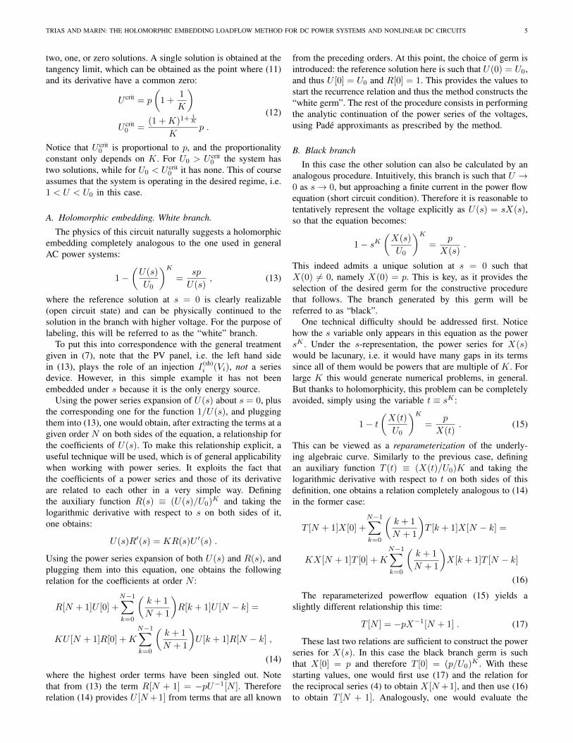
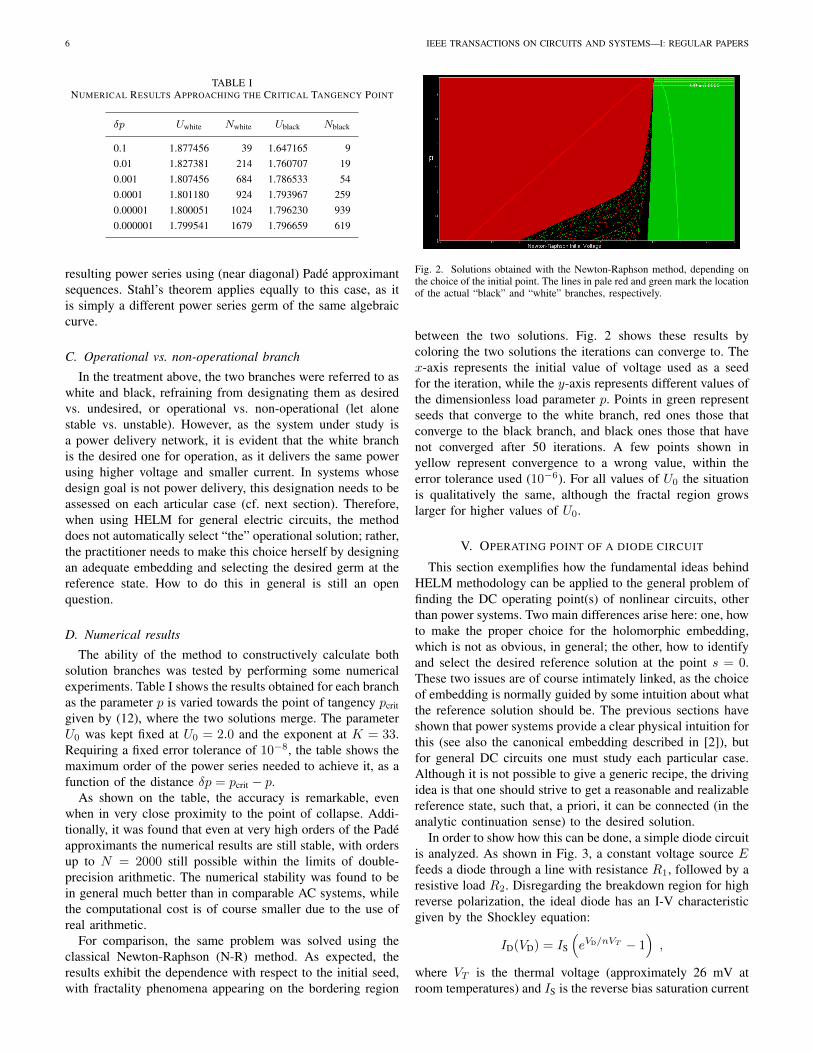
D. Numerical results

The ability of the method to constructively calculate bothsolution branches was tested by performing some numericalexperiments. Table I shows the results obtained for each branchas the parameter p is varied towards the point of tangency pcritgiven by (12), where the two solutions merge. The parameterU0 was kept fixed at U0 = 2.0 and the exponent at K = 33.Requiring a fixed error tolerance of 10−8, the table shows themaximum order of the power series needed to achieve it, as afunction of the distance δp = pcrit − p.

As shown on the table, the accuracy is remarkable, evenwhen in very close proximity to the point of collapse. Addi-tionally, it was found that even at very high orders of the Padeapproximants the numerical results are still stable, with ordersup to N = 2000 still possible within the limits of double-precision arithmetic. The numerical stability was found to bein general much better than in comparable AC systems, whilethe computational cost is of course smaller due to the use ofreal arithmetic.

For comparison, the same problem was solved using theclassical Newton-Raphson (N-R) method. As expected, theresults exhibit the dependence with respect to the initial seed,with fractality phenomena appearing on the bordering region

Fig. 2. Solutions obtained with the Newton-Raphson method, depending onthe choice of the initial point. The lines in pale red and green mark the locationof the actual “black” and “white” branches, respectively.

between the two solutions. Fig. 2 shows these results bycoloring the two solutions the iterations can converge to. Thex-axis represents the initial value of voltage used as a seedfor the iteration, while the y-axis represents different values ofthe dimensionless load parameter p. Points in green representseeds that converge to the white branch, red ones those thatconverge to the black branch, and black ones those that havenot converged after 50 iterations. A few points shown inyellow represent convergence to a wrong value, within theerror tolerance used (10−6). For all values of U0 the situationis qualitatively the same, although the fractal region growslarger for higher values of U0.

V. OPERATING POINT OF A DIODE CIRCUIT

This section exemplifies how the fundamental ideas behindHELM methodology can be applied to the general problem offinding the DC operating point(s) of nonlinear circuits, otherthan power systems. Two main differences arise here: one, howto make the proper choice for the holomorphic embedding,which is not as obvious, in general; the other, how to identifyand select the desired reference solution at the point s = 0.These two issues are of course intimately linked, as the choiceof embedding is normally guided by some intuition about whatthe reference solution should be. The previous sections haveshown that power systems provide a clear physical intuition forthis (see also the canonical embedding described in [2]), butfor general DC circuits one must study each particular case.Although it is not possible to give a generic recipe, the drivingidea is that one should strive to get a reasonable and realizablereference state, such that, a priori, it can be connected (in theanalytic continuation sense) to the desired solution.

In order to show how this can be done, a simple diode circuitis analyzed. As shown in Fig. 3, a constant voltage source Efeeds a diode through a line with resistance R1, followed by aresistive load R2. Disregarding the breakdown region for highreverse polarization, the ideal diode has an I-V characteristicgiven by the Shockley equation:

ID(VD) = IS

(eVD/nVT − 1

),

where VT is the thermal voltage (approximately 26 mV atroom temperatures) and IS is the reverse bias saturation current

TRIAS AND MARIN: THE HOLOMORPHIC EMBEDDING LOADFLOW METHOD FOR DC POWER SYSTEMS AND NONLINEAR DC CIRCUITS 7

R1

1 2

E R2

Fig. 3. Graphical solution of the diode circuit.

(values typically in the µA range). The ideality factor n will betaken to be 1, without losing generality. The circuit equationsare:

E − V1R1

= ID(V1 − V2) =V2R2

. (18)

Since a forward bias E > 0 is assumed, one has 0 < V2 <V1 < E. Defining dimensionless quantities U1 ≡ V1/E,U2 ≡V2/E, u ≡ (V1 − V2)/E, and eliminating U1 from (18), oneobtains:

u = 1−(1 +

R1

R2

)U2 .

Eliminating U2 from (18), and defining the dimensionlessconstants uT ≡ VT /E, ε ≡ (R1 + R2)IS/E, one finallyobtains:

ε(eu/uT − 1

)= 1− u . (19)

It is easy to see graphically that this equation has a singlepositive solution in the interval (0, 1), given by the intersectionof ε(eu/uT − 1) with the line 1− u (see Fig. 3).

In sections III and IV-C it was shown how networksdesigned for power transmission have a natural choice for theembedding and the reference state at s = 0. Here insteadwe are confronted with a general nonlinear DC system, forwhich there is no clear criterion to guide us. This is an openquestion and therefore the best that can be done is to studyit on a case-by-case basis. In our case, looking at (19), thefollowing holomorphic embedding is proposed:

ε(eu(s)/uT − 1

)= 1− su(s) . (20)

This has a well-defined reference state at s = 0, namelyu(0) = uT ln(1 + 1/ε). Additionally, a somewhat physicalinterpretation is possible if one thinks of this embedding asa change u → su(s), uT → suT (this highlights how theintuition driving the design of the embedding is quite differentfrom that used for power systems). Finally, given the shapeof the nonlinearity in (19), it is reasonable to expect thatthe analytic continuation to s = 1 will not encounter anysingularity.

The power series coefficients for u(s) are obtained in ananalogous fashion to the procedures shown in section IV.Defining the auxiliary function E ≡ ε

(eu(s)/uT − 1

), and

taking the derivative with respect to s on both sides of thisdefinition, one obtains:

E′(s) =1

uT(E(s) + ε)u′(s) .

Considering now the power series expansions of E(s) andthe derivatives E′(s), u′(s), one arrives to the followingrelation for the coefficients at order N :

E[N + 1] =E[0] + ε

uTu[N + 1]

+1

uT

N−1∑k=0

(k + 1

N + 1

)u[k + 1]E[N − k] . (21)

Again, the embedded circuit equation (20) provides the othernecessary relation:

E[N + 1] = −u[N ] . (22)

For the reference germ in this case, E[0] = 1 andu[0] = uT ln(1 + 1/ε). Using these starting values one canthus use recurrence relations (21) and (22) to construct thepower series. Numerical experiments on this model show thatthe convergence properties of the resulting Pade approximantsequences are excellent, needing only about N = 5 powerseries terms in order to achieve a relative error of less than10−14. By contrast, Newton-Raphson on this simple systemexhibits widely varying convergence properties depending onthe choice of initial point for the iteration.

VI. COMPARISON WITH ITERATIVE METHODS

A. Conceptual differences. Continuation methods.

In order to address a meaningful and fair comparison withiterative methods, one must first consider the conceptual dif-ferences that separate those from the holomorphic embeddingmethod. At the core of any method based on numericaliteration we find the idea of a map that, when iterated, isexpected to converge to a fixed point. One seeks maps havingthe contraction property, which in principle guarantees thatthe iteration will converge to a fixed point starting from anypoint belonging to a certain (non-empty) set. Such set is calledthe basin of attraction of said fixed point under the map.However, it is well known that these basins of attraction arehard to characterize with precision, as their borders are fractalin general. This problem is particularly relevant for powersystems, where the powerflow equations contain multiplesolutions, each with their own basin of attraction under theiterative scheme. Several authors have explored this fractalityproblem in the context of powerflow [18]–[22], showing withnumerical experiments how the borders between neighboringbasins intertwine in complex patterns, also interspersed withpoints that lead to divergence.

While it is true that in practice the basins of attraction areusually large enough to allow any experimented engineer tofind a good initial point, the issue we want to stress here isthat there is no general procedure to ensure convergence tothe desired solution in a completely unattended fashion, unsu-pervised by any human expert. HELM was actually born out

8 IEEE TRANSACTIONS ON CIRCUITS AND SYSTEMS—I: REGULAR PAPERS

of the need to develop new software applications for decision-support in transmission operation. There, the algorithms relyon performing a massive number of exploratory powerflows,many of them corresponding to abruptly changing scenarios.These algorithms cannot afford that a percentage of cases,however small, has a chance of diverging or mis-convergingto undesired solutions. The same thing would happen to anysort of autonomous control, if it needed to rely on powerflowcalculations.

Many approaches have been developed to minimize thechances of unpredictable behavior in iterative methods, butto our knowledge none of them can guarantee convergencein an automated, unsupervised fashion. This is due to thefundamental fractal behavior underlying contraction mapping-based numerical iteration. Specifically for Newton-Raphson,the Kantorovich theorem does in principle provide a criteriato find out whether a given starting point will converge or not,but this is unusable in practice because it requires computingthe Lipschitz constant of the Jacobian (for a given initialguess), which is highly impractical. Moreover, if the resultwere negative, one would still be left with the hard problemof finding a better initial guess. Additionally, the theorem doesnot say anything about which solution is the desired one.

An important class of methods specifically devised to ad-dress convergence problems are those based on homotopiccontinuation [32]. These path-following methods have beenused both in AC powerflows [33], [34] and for finding theDC operating point of general nonlinear circuits [13]–[15].The apparent similarities between HELM and continuationmethods warrant an extended discussion in order to clarifysome important points. Like HELM, continuation methods arealso based on the general idea of the embedding technique,whereby one is able to solve the problem at the “easy” limitof the embedding parameter (λ = 0) and then follow thissolution up to the value of the parameter where the originalsystem is recovered (λ = 1). However, the key issue is thathomotopy only exploits continuity and single differentiability.It is therefore a local method, essentially. It only requiresthat the starting point satisfies the conditions of the ImplicitFunction Theorem (i.e. no degeneracy at λ = 0), and that nobifurcations are encountered on the path up to λ = 1. Certainbifurcations, namely turning points of the curve with respectto the parameter, may be overcome by switching to arc-lengthparameterization. In the context of finding the DC operatingpoint of nonlinear circuits, probability-1 globally convergentcontinuation methods [13], [35] ensure that no bifurcationswill be encountered (although there is no control as to whatsolution the homotopy arrives to). For these curve-trackingcalculations, methods use either ODE-integration techniquesor a predictor-corrector scheme, where the corrector is basedon Newton-Raphson or quasi-Newton iteration. Modern con-tinuation methods are considered to be computationally slowbut robust, although their reliance on numerical iteration maystill cause problems in practice [34], [36].

In contrast to homotopic continuation, the holomorphicembedding technique exploits holomorphy, in other words,complex analyticity. This is a much stronger condition thansingle differentiability. In fact, holomorphy endows the method

with global properties, because knowledge of the power seriesat a given point (that is, all its derivatives) can be used toreconstruct the function everywhere, by virtue of analytic con-tinuation. It should be emphasized that analytic continuationand homotopic continuation are two different mathematicaltopics that have nothing in common. Analytic continuation isa technique widely used in complex analysis to extend thedomain of a given holomorphic function. In particular, forholomorphic functions given as a power series representation,it is typically used to extend the function beyond the radius ofconvergence of the series. For a general mathematical problem,it is not known a priori what analytic continuation techniquecan be successful (other than a cumbersome re-evaluation ofthe power series at a different point), or what will be the extentof the maximal domain to which the function can be analyt-ically extended. The key point is that, in the context of thepowerflow problem, the HELM method does provide a methodto perform analytic continuation, and moreover, it ensuresthat it is maximal. This analytic continuation is provided bythe sequence of near-diagonal Pade approximants constructedfrom the power series, as established by Stahl’s theorems. Asa way of showing the profound differences with homotopiccontinuation without delving any further in the mathematicalfoundations [2], a few practical differences can be pointed out:HELM is able to directly calculate the solution at any pointalong the embedded path, without needing any previous point,and the calculation is carried out by a constructive procedurein a finite number of steps.

To conclude this discussion on the conceptual differences,a few remarks must be made on a common misunderstandingabout the holomorphic embedding method, regarding its useof power series and “approximants”. In contrast with realanalysis, where Taylor power series have limited use (they arerarely convergent, and may even converge to a value differentthan the function), power series play a major role in complexanalysis, and even more so in the field of algebraic curves. Ac-tually, power series are one of the major ways of representingholomorphic functions. Far from being an approximation, thepower series is the function. And although the power seriesonly converges within its radius of convergence, analytic con-tinuation allows one to make use of the information containedin the the power series to reconstruct the function well beyondthat radius. Note that, for general holomorphic functions,there is no known procedure to obtain the maximal analyticcontinuation, but herein lies the power of Stahl’s theorem:it states that, for the class of functions HELM deals with,the near-diagonal sequences of Pade approximants converge tothe function in their maximal domain of analytic continuation.Therefore, the method is not limited by any convergence issues(within the limits of finite-precision arithmetic), because thesuccessive Pade approximants can get as close as desired tothe sought solution—one just needs to obtain more terms ofthe power series.

B. Analysis of computational performance

In terms of computation, the HELM method for DC systemsconsists of the same overall steps as for AC systems, except

TRIAS AND MARIN: THE HOLOMORPHIC EMBEDDING LOADFLOW METHOD FOR DC POWER SYSTEMS AND NONLINEAR DC CIRCUITS 9

that most of the arithmetic operations work with real variablesinstead of complex ones. The algorithmic structure of theprocedure is as follows:

• Phase 1: factorize the conductance matrix• Phase 2: main loop:

1) Construct the members on the r.h.s. of the recurrentlinear system (see (5) and (8)), using the powerseries terms obtained from the previous N steps.

2) Solve the linear system to obtain the power seriesterms at the next order, N + 1.

3) Use these newly computed terms to calculate thevalue, at s = 1, of the next Pade approximant alongthe stairstep of the Pade table.

4) Check for convergence by comparing the valueswith those obtained from previous steps; if oscil-lation is detected, there is no solution.

To give some idea about the number of steps typicallyneeded in practice, it is found that around 40 to 60 terms of thepower series are sufficient to achieve a numerical precision ofabout 10 significant digits in all but the most ill-conditionedscenarios. Ill-conditioning only happens when the system isextremely close to a branch point (this corresponds to a pointof voltage collapse in power systems), but this condition iseasily detectable: the number of power series terms neededto decide whether there is convergence or oscillation growsabnormally near these points. Actually, in these marginal casesthere are standard techniques of power series analysis thatallow predicting with precision whether the system is “justbefore” or “just beyond” the branching point, independently ofthe Pade calculations. These are seldom needed, unless one isworried about calculating the exact location of collapse pointswith precisions of 10 or more significant digits.

Note how, except for the overhead involved in Phase 2steps 1 and 3, the overall computational complexity of themethod is similar to fast-decoupled powerflow methods [11],[12], since the matrix is factorized only once and its factorsare used repeatedly to solve linear systems (fast decoupledmethods may easily take about 20 to 40 steps or more toconverge, in typical applications). The admittance matricesarising from most networks are very sparse, so it is key touse a good LU sparse solver with fill-reducing permutationsin order to obtain top performance. In our experience, the bestresults are normally obtained with the Approximate MinimumDegree fill-reducing algorithm, together with direct sparse LUsolvers [37]. Note however that multifrontal and supernodalvariants perform worse than the simple ones, because electricnetwork matrices are so sparse that such blocking strategies(driven by the goal of exploiting optimized dense kernels suchas the BLAS) just do not pay off.

Step 1 of Phase 2 involves the calculation of right-hand-side coefficients at order N , using all the power series termspreviously calculated. This typically involves convolutionssuch as the ones appearing in (4), (14), (16), or (21). Thusthe overall work per bus is O(N2), where N is the maximumorder of the power series. Note however that the typical valueof N is relatively low (40 to 60 maximum) and that this workis trivially parallelizable across buses.

Step 3 of Phase 2 involves the calculation of the Padeapproximants for each bus voltage. As discussed in the Ap-pendix, these are computed with algorithms whose cost isorder O(N2) per bus. This cost is for the whole of Phase 2, asthe construction is incremental. Just like step 1, this calculationis trivially parallelizable, as it is completely independent foreach bus. Additionally, for applications where the voltageat only one bus or a few buses is needed, one may avoidthe calculation of the approximants altogether, except for thedesignated buses. This is a very common situation in softwareapplications that perform exploratory powerflows, for instance.Yet another performance tactic is to keep the voltage powerseries and only evaluate the approximants lazily, on demand.

C. Numerical results

For the purposes of comparing HELM to existing methods,we show below the results of some numerical experimentsperformed using a series of medium-size network models. Wehave not tried to test the convergence properties of iterativemethods; as discussed above, the fractal nature of the problemmakes it impossible to obtain any meaningful characterizationvalid for general network models and scenarios, even in astatistical way. Rather, the purpose here is to provide someuseful orders of magnitude about the real-world performanceof HELM vs. iterative the methods, when these converge.

Since our current implementations do not cover yet general(i.e. non-power) DC networks of arbitrary size, the experi-ments have been carried out using standard IEEE test casesfor AC powerflows [38]. As the reduction in computationaleffort resulting from going from AC to DC is expected tobe similar across all methods, we believe the results willstill be informative, at least for DC power systems. Wehave used MATPOWER [39] as a reputable implementationof the standard iterative powerflow methods, and a HELMimplementation written in MATLAB, with no native code op-timizations, for fair comparisons. MATPOWER also containsan implementation of the Continuation Power Flow method,which is capable of using physical parameter homotopies witharc-length and pseudo-arc-length parameterization. It doesnot implement probability-1 globally convergent homotopymethods, but in terms of performance most homotopy methodsshould be similar, as long as no bifurcations are encountered(as it is the case here).

Fig. 4 shows the results of benchmarking the CPU per-formance of our MATLAB-based implementation of HELMagainst Newton-Raphson (NR), Fast Decoupled (FD), andContinuation Power Flow (CPF) methods. The test cases weretaken from the MATPOWER distribution, and range fromthe well-known IEEE test cases [38] to the 9,200 bus testcase from EU Project PEGASE [40]. When benchmarking theiterative algorithms, all cases were solved starting from the“flat start” profile (all buses set to the swing voltage), whichis the best initial guess for power systems. The CPF was set upto perform an homotopy path that resembles the holomorphicembedding as much as possible, i.e. parameterizing load andgenerator injections as λP, λQ. MATPOWER’s CPF did notallow us to interpolate the voltage of PV buses from the

10 IEEE TRANSACTIONS ON CIRCUITS AND SYSTEMS—I: REGULAR PAPERS

case

14

24 ie

ee rt

s

case

30

case

ieee

30

case

39

case

57

case

89pe

gase

case

118

case

300

case

300

PS

case

1354

pega

se

case

2383

wp

case

2736

sp

case

2737

sop

case

2746

wop

case

2746

wp

case

2869

pega

se

case

3012

wp

case

3120

sp

case

3375

wp

case

9241

pega

se

log

t

-2.5

-2

-1.5

-1

-0.5

0

0.5

1

1.5

2

2.5FDXB (tol 10-4)FDXB (tol 10-10)NR (tol 10-4)NR (tol 10-10)HELM (tol 10-4)HELM (tol 10-10)CPF (tol 10-4)CPF (tol 10-10)

Fig. 4. CPU time benchmarks of HELMLAB (a MATLAB implementationof HELM) and various iterative algorithms in MATPOWER.

swing voltage to their respective setpoints, but this is a minordifference and it never prevented convergence. Arc-lengthparameterization and adaptative step-size were used.

With the exception of Gauss-Seidel, which was excludedbecause it failed to converge in more than half of the test cases,all algorithms were verified to converge exactly to the samesolution within the required tolerance. The Fast Decoupledmethod was found to be the fastest in general. For clarity,only the FDXB variant shown, as the FDBX variant showedessentially the same results. The Newton-Raphson method isslightly less performant for large cases, as expected. HELMclocked at speeds about 10 to 50 times slower than NR orFD, although it should be reminded that this code had nooptimizations, other than the use of the stock sparse matrixroutines in MATLAB. The CPF method ran generally theslowest, even with adaptive step-size.

Nevertheless, our experience with high-performance im-plementations written in C has shown that the performanceof HELM is actually much closer to that of NR and FD.CPU profiling indicates that the MATLAB implementation ofHELM suffers from an excessive overhead in Phase 2 steps1 and 3 (see the discussion in the preceding subsection), asthese involve heavily indexed operations that MATLAB cannotvectorize and therefore are run in interpreted mode.

To complete the picture, Fig. 5 provides an idea about thenumber of steps that each algorithm needs to perform as thesize of the model increases and as the required precisionincreases. NR is quite efficient in terms of the number ofiterations, as one expects from its quadratic convergence rate.It achieves a tolerance of 10−4 in about 4–5 iterations andthen it only needs one or two more to reach 10−10 tolerance.FD typically needs more iterations to converge, especiallywhen more precision is required. HELM is shown to requireanywhere from 10 to 20 power series terms in order to achievea tolerance of 10−4, and no more than 35 to 45 to achieve10−10. As discussed above, the only situation where moreterms are needed is when the solution is very close to a pointof collapse. Finally, the CPF shows a heavy increase in thenumber of continuation steps needed as the size of the test

case

14

24 ie

ee rt

s

case

30

case

ieee

30

case

39

case

57

case

89pe

gase

case

118

case

300

case

300

PS

case

1354

pega

se

case

2383

wp

case

2736

sp

case

2737

sop

case

2746

wop

case

2746

wp

case

2869

pega

se

case

3012

wp

case

3120

sp

case

3375

wp

case

9241

pega

se

step

s

0

10

20

30

40

50

60

70

80

90

100

110FDXB (tol 10-4)FDXB (tol 10-10)NR (tol 10-4)NR (tol 10-10)HELM (tol 10-4)HELM (tol 10-10)CPF (tol 10-4)CPF (tol 10-10)

Fig. 5. Number of steps needed by each algorithm in order to attain thedesired precision. Steps are iterations in the case of NR and FD, continuationsteps in CPF, and order of the power series in HELM.

case grows. On the other hand, this number does not dependmuch on the required precision, since its predictor-correctoruses a NR method as the corrector engine.

VII. CONCLUSION

The Holomorphic Embedded Loadflow Method has beenshown to be extensible to DC power systems. Besides constantpower loads, the method can accommodate devices withgeneral nonlinear characteristics, such as those commonlyfound in the onboard power distribution systems of spacecraft,aircraft, and more-electric vehicles. Additionally, the methodcan be extended to the wider problem of finding the DCoperating points of nonlinear electronic circuits.

For power systems, the adaptation to DC has revealed thatHELM’s numerical properties are in general improved overits AC counterpart, even in the presence of highly nonlineardevices. On the theoretical front, DC HELM has also enabledsome new exciting insights and results, some of which alsobenefit AC networks in return.

From the point of view of applications, the most significantadvantage of the method presented here lies in its reliableand deterministic behavior. This derives from its direct andconstructive nature, which completely avoids the dependencyon the choice of an initial point, characteristic of methodsthat rely on numerical iteration. Future lines of work in-clude exploiting this advantage in new intelligent applicationsfor decision-support and autonomous control, for the powermanagement systems of aircraft and spacecraft (especiallyunmanned autonomous vehicles), as well as autonomous DCmicrogids.

On a more fundamental level, non-power DC circuitspresent interesting challenges to explore using this method. Inparticular, more work is needed on the criteria for designingthe holomorphic embedding and the reference state that wouldyield a desired operating point. It is also worth to exploreanalytic continuation techniques other than Pade approximantsapplied to the problem of obtaining all operating points of aDC circuit.

TRIAS AND MARIN: THE HOLOMORPHIC EMBEDDING LOADFLOW METHOD FOR DC POWER SYSTEMS AND NONLINEAR DC CIRCUITS 11

APPENDIX

COMPUTING PADE APPROXIMANTS

Let f(z) be a formal power series:

f(z) = c0 + c1z + c2z2 + · · · =

∞∑N=0

cizN . (23)

The (m,n) Pade approximant of f(z) is defined as the rationalfunction

[m,n]f (z) =Pm,n(z)

Qm,n(z)≡∑m

j=0 pjzj∑n

j=0 qjzj

that satisfies

f(z)− [m,n]f (z) = O(zm+n+1), z → 0. (24)

In other words, it is the fraction of polynomials Pm,n andQm,n, of degrees at most m and n respectively, such thatits Taylor power series coincides with that of f(z) up toorder m + n. The so-called Pade table arranges these intabular form along m rows and n columns, which helpsin revealing symmetries, recurrence formulas between theirvalues, and many other important properties. For instance,there is an intimate relationship between certain continuedfraction representations of f(z) and the “stairstep” sequenceof Pade approximants [1, 1]f , [2, 1]f , [2, 2]f , [3, 2]f , [3, 3]f , . . .Pade approximants are a powerful tool in the arsenal ofnumerical analysts, and have a wide array of theoretical uses incomplex analysis. For general reference, see the review in [41]or the authoritative monograph [27].

In particular, if (23) is a Taylor series representing a functionholomorphic in a neighborhood of z = 0, the Pade approxi-mants can provide one way to obtain the analytic continuationof f(z) for values of z beyond the radius of convergence ofthe power series. For this to work, one first needs to proveconvergence of the Pade approximants to the function, which isnot necessarily true in general. However, in our particular case(functions with branch points), Stahl’s theorem [24] proves thisconvergence, and not only for a restricted region, but over themaximal domain of analytic continuation (though this onlyapplies to near-diagonal sequences of the Pade table).

We now briefly review the landscape of numerical methodsavailable for the calculation of Pade approximants, pointingout whether some specific issues apply or are irrelevant for theparticular Pade approximants needed in HELM. The methodscan divided into two large groups: on the one hand, those thatcompute the coefficients of Pm,n and Qm,n; on the other, thosethat directly obtain the value of the approximant at a givenvalue (in our case, at s = 1). In the context of HELM, onewould normally use the latter, because they are more efficientand have less chance of introducing round-off, as they involveless operations. Still, computing the polynomials might beuseful for analyzing the location of singularities, for instance.

Among algorithms that compute the polynomial coeffi-cients, [27] recommends the straightforward method—solvingthe associated linear system derived from (24) via LU factor-ization with partial pivoting—as a simple and robust strategy.This is has complexity O(n3), which could be of concern forn large, but the bigger issue here is that the Pade table can

have defects: approximants [m,n]f for which the degree of thepolynomials is less than (m,n). In such cases, the correspond-ing linear system is singular. More sophisticated methods,such as the Cabay-Meleshko algorithm [42], automaticallyovercome these problems by means of a look-ahead strategythat efficiently “jumps over” to the next normal (i.e. non-defective) approximant in the Pade table. Additionally, thesemethods exploit the special structure of the matrix (Toepliz);their complexity is O(n2).

Among methods that compute the value of the approx-imant directly, we recommend two: Wynn’s epsilon andRutishauser’s quotient-difference (QD) algorithms. Both ofthese are O(n2), but they are based on fast recurrence relations(related to the Shanks transformation in the case of Wynn, andto continued fractions in the case of QD), so their performanceis excellent in practical applications. A good description ofWynn’s epsilon algorithm can be found in [43], and qualityimplementations appear in [44], [45]. For the QD algorithm,reference [43] contains a brief description, but the reader isadvised to consult the more detailed exposition in [46] forsome important implementation details.

Some careful remarks should be made about the role playedby the so-called Froissart doublets. These are spurious pole-zero pairs appearing in the Pade approximants, having noapparent relationship to the zeros and poles of the analyticfunction. A formal definition of spurious poles has been givenby Stahl [47], who characterizes spuriousness as an asymptoticproperty of the poles. Although Froissart doublets may appearfrom numerical round-off, particularly arising in non-normalblocks of the Pade table, they exist even in exact arithmetic.In fact, they are what prevents local uniform convergence ofPade approximants (at points other than poles or branch cutsof f ) for arbitrary meromorphic functions. But for the classof holomorphic functions involved in HELM, i.e. algebraicfunctions, Stahl’s theorem [24] proves convergence and there-fore Froissart doublets pose no problem. Doublets induced byround-off may still appear, but they disappear or move awayfrom the evaluation point just by increasing the Pade order. Inany case, if one is interested in the detailed study of Froissartdoublets, a recent method published in [48] is reported tohave a remarkable ability to remove spurious doublets. Themethod is based on the Singular Value Decomposition, andhas therefore a complexity of order O(n3).

To conclude this appendix, it is worth mentioning that thereare a few “superfast” O(n log2 n) methods based on divide-and-conquer techniques [49], but in the opinion of some au-thors [50] these do not have a well-established error analysis,compared to most O(n2) methods. Given the relatively lownumber of terms in the power series encountered with HELMin practical settings, the authors have not tried these.

REFERENCES

[1] A. Trias, “The holomorphic embedding load flow method,” in Powerand Energy Society General Meeting, 2012 IEEE, Jul. 2012, pp. 1–8.

[2] A. Trias, “Fundamentals of the Holomorphic Embedding Load-FlowMethod,” ArXiv e-prints, no. 1509.02421, Sep. 2015.

[3] A. Trias, “Sigma algebraic approximants as a diagnostic tool in powernetworks,” US Patent Application 20 140 156 094 A1, Jun., 2014.

12 IEEE TRANSACTIONS ON CIRCUITS AND SYSTEMS—I: REGULAR PAPERS

[4] A. Gomez-Exposito and F. L. Alvarado, “Load flow,” in Electric EnergySystems: Analysis and Operation, A. Gomez-Exposito, A. J. Conejo, andC. Canizares, Eds. CRC Press, 2009, pp. 95–126.

[5] D. Jovcic, D. Van Hertem, K. Linden, J.-P. Taisne, and W. Grieshaber,“Feasibility of DC transmission networks,” in Innovative Smart GridTechnologies (ISGT Europe). IEEE, 2011, pp. 1–8.

[6] A. Willson, Nonlinear networks: theory and analysis, ser. IEEE Pressselected reprint series. IEEE Press, 1975.

[7] L. Chua, C. Desoer, and E. Kuh, Linear and Nonlinear Circuits, ser.Circuits and systems. McGraw-Hill, 1987.

[8] K. J. Metcalf, “Power management and distribution (PMAD) modeldevelopment: Final Report,” NASA Glenn Research Center, Tech. Rep.CR-2011-217268, November 2011.

[9] T. Quarles, D. Pederson, R. Newton, A. Sangiovanni-Vincentelli, andC. Wayne, “SPICE, a general-purpose circuit simulation program,”EECS Department of the University of California at Berkeley.

[10] W. Tinney and C. Hart, “Power flow solution by newton’s method,” IEEETrans. Power App. Syst., vol. PAS-86, no. 11, pp. 1449–1460, 1967.

[11] B. Stott and O. Alsac, “Fast decoupled load flow,” IEEE Trans. PowerApp. Syst., vol. PAS-93, no. 3, pp. 859–869, may 1974.

[12] R. van Amerongen, “A general-purpose version of the fast decoupledload flow,” IEEE Trans. Power Syst., vol. 4, no. 2, pp. 760–770, 1989.

[13] D. M. Wolf and S. R. Sanders, “Multiparameter homotopy methods forfinding DC operating points of nonlinear circuits,” IEEE Trans. CircuitsSyst. I, vol. 43, no. 10, pp. 824–838, 1996.

[14] L. Trajkovic, “Homotopy methods for computing DC operating points,”Wiley Encyclopedia of Electrical and Electronics Engineering, 1999.

[15] ——, “DC operating points of transistor circuits,” Nonlinear Theory andIts Applications, IEICE, vol. 3, no. 3, pp. 287–300, 2012.

[16] D. Crutchley, M. Zwolinski et al., “Globally convergent algorithmsfor DC operating point analysis of nonlinear circuits,” EvolutionaryComputation, IEEE Transactions on, vol. 7, no. 1, pp. 2–10, 2003.

[17] M. H. Zaki, I. M. Mitchell, and M. R. Greenstreet, “DC operatingpoint analysis–A formal approach,” Proceedings of Formal Verificationof Analog Circuits (FAC), 2009.

[18] C. DeMarco and T. Overbye, “Low voltage power flow solutions andtheir role in exit time based security measures for voltage collapse,” in27th IEEE Conference on Decision and Control, 1988, pp. 2127–2131.

[19] J. Thorp and S. Naqavi, “Load flow fractals,” in Proceedings of the 28thIEEE Conference on Decision and Control, vol. 2, 1989, pp. 1822–1827.

[20] ——, “Load-flow fractals draw clues to erratic behaviour,” IEEE Com-put. Appl. Power, vol. 10, no. 1, pp. 59–62, jan 1997.

[21] R. Klump and T. Overbye, “A new method for finding low-voltage powerflow solutions,” in Power Engineering Society Summer Meeting, vol. 1.IEEE, 2000, pp. 593–597.

[22] H. Mori, “Chaotic behavior of the newton-raphson method with the opti-mal multiplier for ill-conditioned power systems,” in IEEE InternationalSymposium on Circuits and Systems (ISCAS), vol. 4, 2000, pp. 237–240.

[23] H. Stahl, “On the convergence of generalized Pade approximants,”Constructive Approximation, vol. 5, pp. 221–240, 1989.

[24] ——, “The convergence of Pade approximants to functions with branchpoints,” J. Approx. Theory, vol. 91, no. 2, pp. 139–204, 1997.

[25] B. Buchberger and F. Winkler, Grobner bases and applications. Cam-bridge University Press, 1998, vol. 251.

[26] I. Niven, “Formal power series,” American Mathematical Monthly,vol. 76, no. 8, pp. 871–889, 1969.

[27] G. Baker and P. Graves-Morris, Pade approximants, ser. Encyclopediaof mathematics and its applications. Cambridge University Press, 1996.

[28] H. Nguyen and K. Turitsyn, “Appearance of multiple stable load flowsolutions under power flow reversal conditions,” in PES General Meeting— Conference Exposition, 2014 IEEE, July 2014, pp. 1–5.

[29] Y. Tamura, H. Mori, and S. Iwamoto, “Relationship between voltageinstability and multiple load flow solutions in electric power systems,”IEEE Trans. Power App. Syst., no. 5, pp. 1115–1125, 1983.

[30] B. H. Cho, J. R. Lee, and F. C. Lee, “Large-signal stability analysisof spacecraft power processing systems,” IEEE Trans. Power Electron.,vol. 5, no. 1, pp. 110–116, 1990.

[31] Y. H. Lim and D. C. Hamill, “Nonlinear phenomena in a modelspacecraft power system,” in 6th IEEE Workshop on Computers in PowerElectronics (COMPEL), 1998, pp. 169–175.

[32] E. Allgower and K. Georg, Introduction to numerical continuationmethods, ser. Classics in applied mathematics. SIAM, 2003.

[33] V. Ajjarapu and C. Christy, “The continuation power flow: a tool forsteady state voltage stability analysis,” IEEE Trans. Power Syst., vol. 7,no. 1, pp. 416–423, feb 1992.

[34] J. Zaborsky and M. Ilic, Dynamics and Control of Large Electric PowerSystems. Wiley-IEEE Press, 2000.

[35] R. C. Melville, L. Trajkovic, S.-C. Fang, and L. T. Watson, “Artificialparameter homotopy methods for the DC operating point problem,”IEEE Trans. Comput.-Aided Design Integr. Circuits Syst., vol. 12, no. 6,pp. 861–877, 1993.

[36] J. Roychowdhury and R. Melville, “Delivering global DC convergencefor large mixed-signal circuits via homotopy/continuation methods,”IEEE Trans. Comput.-Aided Design Integr. Circuits Syst., vol. 25, no. 1,pp. 66–78, 2006.

[37] T. Davis, Direct methods for sparse linear systems, ser. Fundamentalsof algorithms. SIAM, 2006.

[38] R. D. Christie, “Power systems test case archive,” Universityof Washington. [Online]. Available: https://www.ee.washington.edu/research/pstca/

[39] R. Zimmerman, C. Murillo-Sanchez, and R. Thomas, “MATPOWER:steady-state operations, planning, and analysis tools for power systemsresearch and education,” IEEE Trans. Power Syst., vol. 26, no. 1, pp.12–19, Feb 2011.

[40] S. Fliscounakis, P. Panciatici, F. Capitanescu, and L. Wehenkel, “Con-tingency ranking with respect to overloads in very large power systemstaking into account uncertainty, preventive, and corrective actions,” IEEETrans. Power Syst., vol. 28, no. 4, pp. 4909–4917, 2013.

[41] W. B. Gragg, “The Pade table and its relation to certain algorithms ofnumerical analysis,” SIAM Review, vol. 14, no. 1, pp. 1–62, 1972.

[42] S. Cabay and R. Meleshko, “A weakly stable algorithm for Padeapproximants and the inversion of hankel matrices,” SIAM Journal onMatrix Analysis and Applications, vol. 14, no. 3, pp. 735–765, 1993.

[43] A. Sidi, Practical Extrapolation Methods: Theory and Applications.Cambridge University Press, 2003.

[44] E. J. Weniger, “Nonlinear sequence transformations for the accelerationof convergence and the summation of divergent series,” ComputerPhysics Reports, vol. 10, no. 5, pp. 189–371, 1989.

[45] W. Press, Numerical Recipes 3rd Edition: The Art of Scientific Comput-ing. Cambridge University Press, 2007.

[46] P. Henrici, Applied and Computational Complex Analysis, Vols 1–3, ser.Wiley Classics Library (Book 43). Wiley-Interscience, 1993.

[47] H. Stahl, “Spurious poles in Pade approximation,” Journal of computa-tional and applied mathematics, vol. 99, no. 1, pp. 511–527, 1998.

[48] P. Gonnet, S. Guttel, and L. N. Trefethen, “Robust Pade approximationvia SVD,” SIAM review, vol. 55, no. 1, pp. 101–117, 2013.

[49] R. P. Brent, F. G. Gustavson, and D. Y. Yun, “Fast solution of Toeplitzsystems of equations and computation of Pade approximants,” Journalof Algorithms, vol. 1, no. 3, pp. 259–295, 1980.

[50] B. Beckermann and G. Labahn, “Effective computation of rationalapproximants and interpolants,” Reliable Computing, vol. 6, no. 4, pp.365–390, 2000.

Antonio Trias received a PhD degree in Physicsfrom the University of Barcelona in 1974. From1974 to 1976 he was a visiting postdoctoral researchfellow at the Lawrence Berkeley Laboratory of theUniversity of California. He is a founding member ofAplicaciones en Informatica Avanzada S.A., wherehe currently is R&D Vice President and CTO. Hehas worked in the load flow problem and otheralgorithms of interest for power systems for overtwenty years.

Jose Luis Marın received a PhD degree in Physicsfrom the University of Zaragoza in 1997. He hasbeen a postdoc research assistant at the Universityof Cambridge and at CEA Saclay, and a Marie Curieresearch fellow at Heriot-Watt University. In 2005 hejoined Grupo AIA, where he has worked on analyticapplications for power systems and other industrialproblems in the utility sector. He is currently withthe subsidiary Gridquant Espana, working on thedevelopment of HELM-based commercial tools.