IEEE TRANSACTIONS ON COMPUTERS, JANUARY … (e.g. software bugs) and external (e.g. resource exhaustion) impairments. These chronic problems often ﬂy under the radar of software

IEEE TRANSACTIONS ON COMPUTERS, JANUARY 2015 1

CHAOS: Accurate and Realtime Detection ofAging-Oriented Failure Using Entropy

Pengfei Chen,Yong Qi, Member, IEEE,and Di Hou,

Abstract—Even well-designed software systems suffer from chronic performance degradation, also named “software aging”, due tointernal (e.g. software bugs) and external (e.g. resource exhaustion) impairments. These chronic problems often fly under the radar ofsoftware monitoring systems before causing severe impacts (e.g. system failure). Therefore it’s a challenging issue how to timely detectthese problems to prevent system crash. Although a large quantity of approaches have been proposed to solve this issue, the accuracyand effectiveness of these approaches are still far from satisfactory due to the insufficiency of aging indicators adopted by them. In thispaper, we present a novel entropy-based aging indicator, Multidimensional Multi-scale Entropy (MMSE). MMSE employs the complexityembedded in runtime performance metrics to indicate software aging and leverages multi-scale and multi-dimension integration totolerate system fluctuations. Via theoretical proof and experimental evaluation, we demonstrate that MMSE satisfies Stability,Monotonicity and Integration which we conjecture that an ideal aging indicator should have. Based upon MMSE, we develop threefailure detection approaches encapsulated in a proof-of-concept named CHAOS. The experimental evaluations in a Video on Demand(VoD) system and in a real-world production system, AntVision, show that CHAOS can detect the failure-prone state in anextraordinarily high accuracy and a near 0 Ahead-Time-To-Failure (ATTF ). Compared to previous approaches, CHAOS improves thedetection accuracy by about 5 times and reduces the ATTF even by 3 orders of magnitude. In addition, CHAOS is light-weight enoughto satisfy the realtime requirement.

Index Terms—Software aging, Multi-scale entropy, Failure detection, Availability.

F

1 INTRODUCTION

Software is becoming the backbone of modern society.Especially with the development of cloud computing, moreand more traditional services (e.g. food ordering, retail) aredeployed in the cloud and function as distributed soft-ware systems. Two common characteristics of those soft-ware systems, namely long-running and high complexityincrease the risks of faults and resource exhaustion. With theaccumulation of faults or resource consumption, softwaresystems may suffer from chronic performance degradation,failure rate/probability increase and even crash called “soft-ware aging” [1], [2], [3], [4], [5] or “Chronics” [6].

Software aging has been extensively studied for twodecades since it was first quantitatively analyzed in AT&Tlab in 1995 [7]. This phenomenon has been widely observedin variant software systems nearly spanning across all soft-ware stacks such as cloud computing infrastructure (e.g. Eu-calyptus) [8], [9], virtual machine monitor (VMM) [10], [11],operating system [1], [12], Java Virtual Machine (JVM) [5],[13], web server [4], [14] and so on. As the degree of softwareaging increasing, software performance decreases graduallyresulting in QoS (e.g. response time) decrease. What’s worse,software aging may lead to unplanned system hang orcrash The unplanned outage in enterprise system especiallyin cloud platform can cause considerable revenue loss. Arecent survey shows that IT downtime on an average leadsto 14 hours of downtime per year, leading to $26.5 billionlost [15]. Therefore detecting and counteracting softwareaging are of essence for building long-running systems.

• P.Chen, Y.Qi and D.Hou are with the Department of Computer Scienceand Technology, Xi’an Jiaotong University, Xi’an, China, 710049.E-mail: [email protected]

An efficient and commonly used counteracting softwareaging strategy is “software rejuvenation” [3], [4], [5], [16],which proactively recovers the system from failure-pronestate to a completely or partially new state by cleaning theinternal state. The benefit of rejuvenation strategies heavilydepends on the time triggering rejuvenation. Frequent re-juvenation actions may decrease the system availability orperformance due to the non-ignorable planed downtime oroverhead caused by such actions. Instead, an ideal rejuve-nation strategy is to recover the system when it just getsnear to the failure-prone state.We name the failure-pronestate caused by software aging as “Aging-Oriented Fail-ure”(AOF). Different from transient failures caused by fatalerrors e.g. segment fault or hardware failures, AOF is a kindof “chronics” [6] which means some durable anomalies haveemerged before system crash. Therefore AOF is likely to bedetected. Accurately detecting AOF is a critical problem andthe goal of this paper. However, to that end, we confront thefollowing three challenges:

• Different from fail-stop problems e.g. crash or hangwhich have sufficient and observable indicators (e.g.exceptions), non-crash failures caused by softwareaging where the server does not crash but fails toprocess the request compliant with the SLA con-straints, have no observable and sufficient symptomsto indicate them. These failures often fly under theradar of monitoring systems. Hence, finding out theunderlying indicator for software aging becomes thefirst challenge.

• The internal state (e.g. memory leak) changes andexternal state (e.g. workload variation) changes makethe running system extraordinarily complex. Hence,

arX

iv:1

502.

0078

1v1

[cs

.OH

] 3

Feb

201

5


the running system may not be described neitherby a simple linear model nor by a single perfor-mance metric. How to cover the complexity andmulti-dimension in the aging indicator is the secondchallenge.

• Fluctuations or noise may be involved in collectedperformance metrics due to the highly dynamicproperty of the running system. And cloud comput-ing exacerbates the dynamics due to its elasticity andflexibility (e.g. VM creation and deletion). How tomitigate the influence of noise and keep the detectionapproach noise-resilient is the third challenge.

To address the aforementioned challenges, we conjecturethat an ideal aging indicator should have Monotonicity prop-erty to reveal the hidden aging state, Integration propertyto comprehensively describe aging process and Stabilityproperty to tolerate system fluctuation. In this paper, wepropose a novel aging indicator named MMSE. Accordingto our observation in practice and qualitative proof, entropymonotonously increases with the degree of software agingwhen the failure probability is lower than 0.5. And MMSEis a complexity oriented and model-free indicator withoutdeterministic linear or non-linear model assumptions. Inaddition, the multi-scale feature mitigates the influence ofsystem fluctuations and the multi-dimension feature makesMMSE more comprehensive to describe software aging.Hence, MMSE satisfies the three properties namely Stability,Monotonicity and Integration, which we conjecture that anideal aging indicator should have. Based upon MMSE, wedevelop three AOF detection approaches encapsulated in aproof-of-concept, CHAOS. To further decrease the overheadcaused by CHAOS, we reduce the runtime performancemetrics from 76 to 5 without significant information lossby a principal component analysis (PCA) based variableselection method. The experimental evaluations in a VoDsystem and in a real production system, AntVision 1, showthat CHAOS has a strong power to detect failure-prone statewith a high accuracy and a small ATTF . Compared toprecious approaches CHAOS increases the detection accu-racy by about 5 times and reduces the ATTF significantlyeven by 3 orders of magnitude. According to our bestknowledge, this is the first work to leverage entropy toindicator software aging. The contribution of this paper isthree-fold:

• We demonstrate that entropy increases with softwareaging and verify this conclusion via experimentalpractice and quantitative proof.

• We propose a novel aging indicator named MMSE.MMSE employs the complexity embedded in mul-tiple runtime performance metrics to measure soft-ware aging and leverages multi-scale and multi-dimension integration to tolerate system fluctuations,which makes MMSE satisfy the properties: Stability,Monotonicity and Integration.

• We design and implement a proof-of-concept namedCHAOS, and evaluate the accuracy of three failuredetection approaches based upon MMSE encapsu-lated in CHAOS in a VoD system and a real pro-duction system, AntVision. The experimental results

1. www.antvision.net

show that CHAOS improves the detection accuracyby about 5 times and reduces the ATTF by 3 ordersof magnitude compared to previous approaches.

The rest of this paper is organized as follows. We demon-strate the motivations of this paper in Section II. SectionIII shows our solution to detect the failure-prone state andthe overview of CHAOS. And in Section IV, we describethe detailed design of CHAOS including: metric selection,MSE and MMSE calculation procedure, and failure-pronestate detection approaches. Section V shows the evaluationresults and comparisons to previous approaches. In SectionVI we state the related work briefly. Section VII concludesthis paper.

2 MOTIVATION

The accuracy of Aging-Oriented Failure (AOF) detectionapproaches is largely determined by the aging indicators.A well-designed aging indicator can precisely indicate theAOF. If the subsequent rejuvenations are always conductedat the real failure-prone state, the rejuvenation cost willtend to be optimal. But unfortunately, prior detection ap-proaches based upon explicit aging indicators [1], [2], [4],[5], [14], [17], [18] don’t function well especially in theface of dynamic workloads. They either miss some failuresleading to a low recall or mistake some normal states as thefailure states leading to a low precision. The insufficiencyof previous indicators motivates us to seek novel indicators.We describe our motivations from the following aspects.

2.1 Insufficiency of Explicit Aging IndicatorsTo distinguish the normal state and failure-prone state, athreshold should be preset on the aging indicator. Once theaging indicator exceeds the threshold, a failure occurs. Tra-ditionally, a threshold is set on explicit aging indicators. Forinstance, if the CPU utilization exceeds 90%, a failure occurs.However, it’s not always the case. The external observationsdo not always reveal accurately the internal states. Here theinternal states can be referred to as some normal events(e.g. a file reading, a packet sending) or abnormal events(e.g. a file open exception, a round-off error) generated inthe system. In this paper we are more concerned aboutthe abnormal events. Commonly, the internal state spaceis much smaller than the directly observed external statespace. For example, the observed CPU utilization can be anyreal number in the range 0% ∼ 100% while the abnormalevents are very limited. Therefore an abnormal event maycorrelate with multiple observations. Still take the CPU uti-lization for example. When a failure-prone event happens,the CPU utilization may be 99%, 80% or even 10%. Thereforethe explicit aging indicator can not signify AOF sufficientlyand accurately. And if the system fluctuation is taken intoaccount, the situation may get even worse. And this is alsoa reason why it’s so difficult to set an optimal threshold onthe explicit aging indicators in order to obtain an accuratefailure detection result.

2.2 Entropy Increase in VoD SystemAs the explicit aging indicators fall short in detecting Aging-Oriented Failure, we turn to implicit aging indicators for


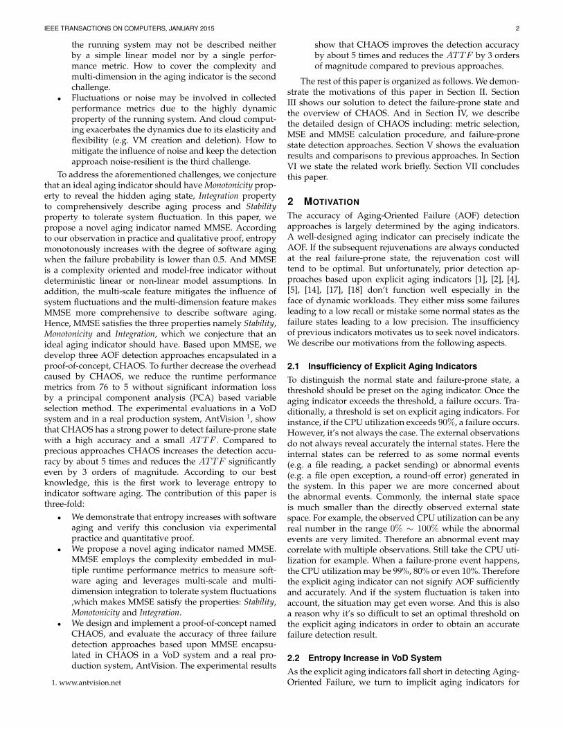
Fig. 1. The CPU utilization of a real VoD system. In this figure, we onlyshow the CPU utilization of the first four days and the last four days.

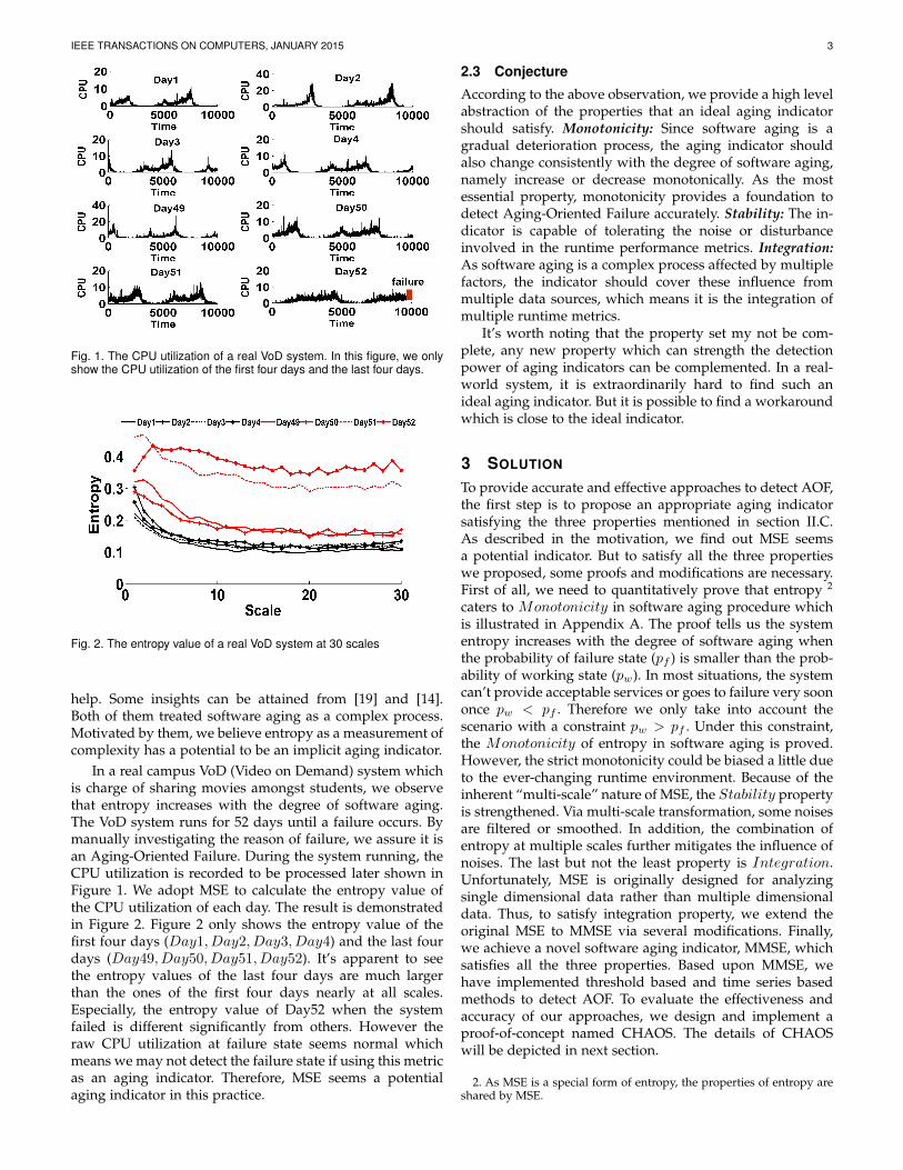
Fig. 2. The entropy value of a real VoD system at 30 scales

help. Some insights can be attained from [19] and [14].Both of them treated software aging as a complex process.Motivated by them, we believe entropy as a measurement ofcomplexity has a potential to be an implicit aging indicator.

In a real campus VoD (Video on Demand) system whichis charge of sharing movies amongst students, we observethat entropy increases with the degree of software aging.The VoD system runs for 52 days until a failure occurs. Bymanually investigating the reason of failure, we assure it isan Aging-Oriented Failure. During the system running, theCPU utilization is recorded to be processed later shown inFigure 1. We adopt MSE to calculate the entropy value ofthe CPU utilization of each day. The result is demonstratedin Figure 2. Figure 2 only shows the entropy value of thefirst four days (Day1, Day2, Day3, Day4) and the last fourdays (Day49, Day50, Day51, Day52). It’s apparent to seethe entropy values of the last four days are much largerthan the ones of the first four days nearly at all scales.Especially, the entropy value of Day52 when the systemfailed is different significantly from others. However theraw CPU utilization at failure state seems normal whichmeans we may not detect the failure state if using this metricas an aging indicator. Therefore, MSE seems a potentialaging indicator in this practice.

2.3 Conjecture

According to the above observation, we provide a high levelabstraction of the properties that an ideal aging indicatorshould satisfy. Monotonicity: Since software aging is agradual deterioration process, the aging indicator shouldalso change consistently with the degree of software aging,namely increase or decrease monotonically. As the mostessential property, monotonicity provides a foundation todetect Aging-Oriented Failure accurately. Stability: The in-dicator is capable of tolerating the noise or disturbanceinvolved in the runtime performance metrics. Integration:As software aging is a complex process affected by multiplefactors, the indicator should cover these influence frommultiple data sources, which means it is the integration ofmultiple runtime metrics.

It’s worth noting that the property set my not be com-plete, any new property which can strength the detectionpower of aging indicators can be complemented. In a real-world system, it is extraordinarily hard to find such anideal aging indicator. But it is possible to find a workaroundwhich is close to the ideal indicator.

3 SOLUTION

To provide accurate and effective approaches to detect AOF,the first step is to propose an appropriate aging indicatorsatisfying the three properties mentioned in section II.C.As described in the motivation, we find out MSE seemsa potential indicator. But to satisfy all the three propertieswe proposed, some proofs and modifications are necessary.First of all, we need to quantitatively prove that entropy 2

caters to Monotonicity in software aging procedure whichis illustrated in Appendix A. The proof tells us the systementropy increases with the degree of software aging whenthe probability of failure state (pf ) is smaller than the prob-ability of working state (pw). In most situations, the systemcan’t provide acceptable services or goes to failure very soononce pw < pf . Therefore we only take into account thescenario with a constraint pw > pf . Under this constraint,the Monotonicity of entropy in software aging is proved.However, the strict monotonicity could be biased a little dueto the ever-changing runtime environment. Because of theinherent “multi-scale” nature of MSE, the Stability propertyis strengthened. Via multi-scale transformation, some noisesare filtered or smoothed. In addition, the combination ofentropy at multiple scales further mitigates the influence ofnoises. The last but not the least property is Integration.Unfortunately, MSE is originally designed for analyzingsingle dimensional data rather than multiple dimensionaldata. Thus, to satisfy integration property, we extend theoriginal MSE to MMSE via several modifications. Finally,we achieve a novel software aging indicator, MMSE, whichsatisfies all the three properties. Based upon MMSE, wehave implemented threshold based and time series basedmethods to detect AOF. To evaluate the effectiveness andaccuracy of our approaches, we design and implement aproof-of-concept named CHAOS. The details of CHAOSwill be depicted in next section.

2. As MSE is a special form of entropy, the properties of entropy areshared by MSE.


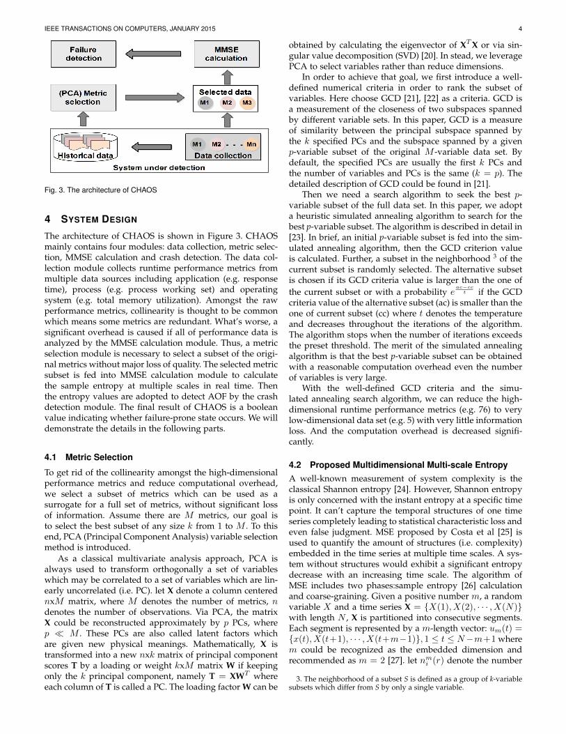
Fig. 3. The architecture of CHAOS

4 SYSTEM DESIGN

The architecture of CHAOS is shown in Figure 3. CHAOSmainly contains four modules: data collection, metric selec-tion, MMSE calculation and crash detection. The data col-lection module collects runtime performance metrics frommultiple data sources including application (e.g. responsetime), process (e.g. process working set) and operatingsystem (e.g. total memory utilization). Amongst the rawperformance metrics, collinearity is thought to be commonwhich means some metrics are redundant. What’s worse, asignificant overhead is caused if all of performance data isanalyzed by the MMSE calculation module. Thus, a metricselection module is necessary to select a subset of the origi-nal metrics without major loss of quality. The selected metricsubset is fed into MMSE calculation module to calculatethe sample entropy at multiple scales in real time. Thenthe entropy values are adopted to detect AOF by the crashdetection module. The final result of CHAOS is a booleanvalue indicating whether failure-prone state occurs. We willdemonstrate the details in the following parts.

4.1 Metric Selection

To get rid of the collinearity amongst the high-dimensionalperformance metrics and reduce computational overhead,we select a subset of metrics which can be used as asurrogate for a full set of metrics, without significant lossof information. Assume there are M metrics, our goal isto select the best subset of any size k from 1 to M . To thisend, PCA (Principal Component Analysis) variable selectionmethod is introduced.

As a classical multivariate analysis approach, PCA isalways used to transform orthogonally a set of variableswhich may be correlated to a set of variables which are lin-early uncorrelated (i.e. PC). let X denote a column centerednxM matrix, where M denotes the number of metrics, ndenotes the number of observations. Via PCA, the matrixX could be reconstructed approximately by p PCs, wherep � M . These PCs are also called latent factors whichare given new physical meanings. Mathematically, X istransformed into a new nxk matrix of principal componentscores T by a loading or weight kxM matrix W if keepingonly the k principal component, namely T = XWT whereeach column of T is called a PC. The loading factor W can be

obtained by calculating the eigenvector of XTX or via sin-gular value decomposition (SVD) [20]. In stead, we leveragePCA to select variables rather than reduce dimensions.

In order to achieve that goal, we first introduce a well-defined numerical criteria in order to rank the subset ofvariables. Here choose GCD [21], [22] as a criteria. GCD isa measurement of the closeness of two subspaces spannedby different variable sets. In this paper, GCD is a measureof similarity between the principal subspace spanned bythe k specified PCs and the subspace spanned by a givenp-variable subset of the original M -variable data set. Bydefault, the specified PCs are usually the first k PCs andthe number of variables and PCs is the same (k = p). Thedetailed description of GCD could be found in [21].

Then we need a search algorithm to seek the best p-variable subset of the full data set. In this paper, we adopta heuristic simulated annealing algorithm to search for thebest p-variable subset. The algorithm is described in detail in[23]. In brief, an initial p-variable subset is fed into the sim-ulated annealing algorithm, then the GCD criterion valueis calculated. Further, a subset in the neighborhood 3 of thecurrent subset is randomly selected. The alternative subsetis chosen if its GCD criteria value is larger than the one ofthe current subset or with a probability e

ac−cct if the GCD

criteria value of the alternative subset (ac) is smaller than theone of current subset (cc) where t denotes the temperatureand decreases throughout the iterations of the algorithm.The algorithm stops when the number of iterations exceedsthe preset threshold. The merit of the simulated annealingalgorithm is that the best p-variable subset can be obtainedwith a reasonable computation overhead even the numberof variables is very large.

With the well-defined GCD criteria and the simu-lated annealing search algorithm, we can reduce the high-dimensional runtime performance metrics (e.g. 76) to verylow-dimensional data set (e.g. 5) with very little informationloss. And the computation overhead is decreased signifi-cantly.

4.2 Proposed Multidimensional Multi-scale EntropyA well-known measurement of system complexity is theclassical Shannon entropy [24]. However, Shannon entropyis only concerned with the instant entropy at a specific timepoint. It can’t capture the temporal structures of one timeseries completely leading to statistical characteristic loss andeven false judgment. MSE proposed by Costa et al [25] isused to quantify the amount of structures (i.e. complexity)embedded in the time series at multiple time scales. A sys-tem without structures would exhibit a significant entropydecrease with an increasing time scale. The algorithm ofMSE includes two phases:sample entropy [26] calculationand coarse-graining. Given a positive number m, a randomvariable X and a time series X = {X(1), X(2), · · · , X(N)}with length N , X is partitioned into consecutive segments.Each segment is represented by a m-length vector: um(t) ={x(t), X(t+1), · · · , X(t+m−1)}, 1 ≤ t ≤ N−m+1 wherem could be recognized as the embedded dimension andrecommended as m = 2 [27]. let nmi (r) denote the number

3. The neighborhood of a subset S is defined as a group of k-variablesubsets which differ from S by only a single variable.


of segments that satisfy d(um(i), um(j)) ≤ r, i 6= j wherei 6= j guarantees that self-matches are excluded, r is a presetthreshold indicating the tolerance level for two segments tobe considered similar and recommended as r = 1.5 ∗ σ [27]where σ is the standard deviation of the original time series.d(·) = max{|X(i+ k)−X(j + k)| : 1 ≤ k ≤ m− 1} repre-sents the maximum of the absolute values of differences be-tween um(i), um(j) measured by Euclidean distance whichis adopted in this paper Let lnCmi (r) = lnum(i)

N−m representthe natural logarithm of the probability that any segmentum(j) is close to segment um(i), the average of lnCm(r) isexpressed as:

Φm(r) =

∑N−m+1i lnCmi (r)

N −m+ 1(1)

The sample entropy is formalized as:

SE(m, r,N) = −lnΦm+1(r)

Φm(r)(2)

To ensure Φm+1(r) is defined in any particular N -lengthtime series, sample entropy redefines Φm(r) as:

Φm(r) =

∑N−mi lnCmi (r)

N −m(3)

Suppose τ is the scale factor, the consecutive coarse-grained time series Y τ is constructed in the following twosteps:

• Divide the original time series X into consecutive andnon-overlapping windows of length τ ;

• Average the data points inside each window;

Finally we get Y τ = {yτj | : 1 ≤ j ≤ bNτ c} and each elementof Y τ is defined as:

yτj =

∑jτi=(j−1)τ+1X(i)

τ, 1 ≤ j ≤ bN

τc (4)

When τ = 1, Y τ degenerates to the original time seriesX. Then MSE of the original time series X is obtained bycomputing the sample entropy of Y τ at all scales. However,the conventional MSE is designed for single dimensionalanalysis. Thus, it doesn’t satisfy the property Integration ofan aging indicator. To this end, we extend MSE to MMSEvia several modifications.

Modification 1. The collected multi-dimensional perfor-mance metrics usually have different scales and numericalranges. For example the CPU utilization metric stays inthe range of 0 ∼ 100 percentage while the total memoryutilization may vary in the range 1048576KB ∼ 4194304 KB.Thus, the distance between two segments may be biasedby the performance metrics with large numerical ranges,which further results in MSE bias. To avoid that bias, wenormalize all the performance metrics to a unified numericalrange,namely 0 ∼ 1. Suppose X is a Nxp data matrix wherep is the number of performance metrics, N is the lengthof the data window and each column of X denotes thetime series of one particular performance metric, then Xis normalized in the following way:

X′

ji =Xji −min(Xi)

max(Xi)−min(Xi), 1 ≤ i ≤ p, 1 ≤ j ≤ N (5)

Modification 2. In MSE algorithm, we quantify thesimilarity between two segments via maximum norm [28]of two scalar numbers. A novel quantification approach isnecessary when MSE is extended to MMSE. Each elementin the maximal norm pair: max{|X(i + k) − X(j + k)| :1 ≤ k ≤ m − 1} such as X(i + k) is replaced by a vectorX(i + k) where each element represents the observation ofone specific performance metric at time i+k. Thus the scalarnorm is transformed to the vector norm. The embeddeddimension m should also be vectorized when the analysisshifts from single dimension to multiple dimensions. Thevectorization brings a nontrivial problem in the calculationprocedure of sample entropy that is how to obtain φm+1(r).Assume that the embedding vector m = (m1,m2, · · · ,mp)denotes the embedded dimensions for p performance met-rics respectively. A new embedding vector m+ which hasone additional dimension compared to m can be obtainedin two ways. The first approach comes from the study in[28]. According to the embedding theory mentioned in [29],m+ can be achieved by adding one additional dimension toonly one specific embedded dimension in m, which leadsto p different alternatives. m+ can be any one of the set{(m1,m2, · · · ,mk + 1, · · · ,mp), 1 ≤ k ≤ p}. φm+

(r) is cal-culated in a naive way or a rigorous way both of which aredepicted in detail in [28]. The other approach is very simpleand intuitional that is adding one additional dimension toevery embedded dimension in m. There is only one alterna-tive for m+ namely {(m1 + 1,m2 + 1, · · · ,mk + 1, · · · ,mp +1), 1 ≤ k ≤ p} . This simple approach implies that eachembedded dimension is identical, which may be a strongconstraint. However, compared to the former approach, thelatter one has negligible computation overhead and workswell in this paper. The former approach will be discussed inour future work.

Modification 3. In MSE algorithm, the threshold r isset as r = 0.15 ∗ σ.In MMSE algorithm, we need a singlenumber to represent the variance of the multi-dimensionalperformance data in order to apply it directly in the sim-ilarity calculation procedure. Here we employ the totalvariance denoted by tr(S) which is defined as the traceof the covariance S of the normalized multi-dimensionalperformance data to replace σ.

Modification 4. We argue that an ideal aging indicatorshould be expressed as a single number in order to be read-ily used in failure detection. The output of the conventionalMSE is a vector of entropy values at multiple scales. Weneed to use a holistic metric to integrate all the entropyvalues at multiple scales. Thus a composed entropy (CE) isproposed. Let T denote the number of scales and the vectorE = (e1, e2, · · · , eT ) denote the entropy value at each scalerespectively. Then CE is defined as the Euclidean norm ofthe entropy vector E :

CE = 2

√√√√ T∑i=1

e2i (6)

CE cloud be regarded as the Euclidean distance betweenE and a “zero” entropy vector which consists of 0 entropyvalues. A “zero” entropy vector represents an ideal systemstate meaning that the system runs in a health state withoutany fluctuations. Thus the more E deviates from a “zero”


entropy vector, the worse the system performance is. It’sworth noting that CE is not the unique metric which canintegrate the entropy values at all scales. Other metrics alsohave the potential to be the aging indicators. For example,the average of E is another alternative although we observethat it has a consistent result with CE.

Through the aforementioned modifications on MSE, thenovel aging indicator MMSE has satisfied all the threeproperties: Monotonicity, Stability and Integration proposedin Section II.C. For the sake of clarity, we demonstrate thepseudo code of MMSE algorithm in Algorithm 1.

Algorithm 1 MMSE algorithmInput: m:the embedded dimension; T :the number of

scales; N :the length of data window; X: a Nxp datamatrix where each p denotes the number of performancemetrics and each column Xi, 1 ≤ i ≤ p denotes the timeseries of one specific performance metric with length N .

Output: The aging degree metric CE1: // Normalize the original time series into the range [0,1]

2: for j = 1; j = N ; j + + do3: for i = 1; i = p; i+ + do4: X

′

ji =Xji−min(Xi)

max(Xi)−min(Xi)5: end for6: end for7: // Preset the similarity threshold r8: S = Cov(X

′) // Cov denotes the matrix covariance

9: r = tr(S) // tr denotes the trace of a particular matrix10: for τ = 1; τ = T ; τ + + do11: // Coarse-graining procedure12: for i = 1; i = p; i+ + do13: for j = 1; j = bNτ c; j + + do

14: Yji =

∑jτ

k=(j−1)τ+1X′ki

τ15: end for16: end for17: E(τ) = ExtendedSampleEntropy(m, r, Y )18: // The similarity calculation between two19: // segments has been extended from scalar20: // to vector in ExtendedSampleEntropy(·)21: end for22: // Calculate the composed entropy CE

23: CE = 2

√∑Ti=1E(i)2

4.3 AOF Detection based upon MMSEBased upon the proposed aging indicator MMSE, it’s easy todesign algorithms to detect AOF in real time. According tothe survey [30], there are three kinds of approaches includ-ing time series analysis,threshold-based and machine learning todetect or predict the occurrence of AOF.In this paper, weonly discuss the time series and threshold-based approachesand leave the machine learning approach in our futurework. But before that we need to determine a sliding datawindow in order to calculate MMSE in real time. As men-tioned in previous work [31], bNτ c should stay in the range10m to 30m. Thus the sliding window heavily depends onthe scale factor τ . In previous studies [25], [28], [32], theyusually set the scale factor τ in the range 1 ∼ 20 leading to

a huge data window, say 10000, especially when τ = 20. Alarge sliding window not only increases the computationaloverhead but also makes detection approaches insensitiveto failure. Thus we constrain the sliding window in anappropriate range, say no more than 1000, by limiting therange of τ . In this paper we set τ in the range 1 ∼ 10.So a moderate data window N = 1000 can cater the basicrequirement.Threshold based approach. As a simple and straightfor-ward approach, the threshold based approach is widelyused in aging failure detection [33], [34]. If the aging indica-tor exceeds the preset threshold, a failure occurs. Howeveran essential challenge is how to identify an appropriatethreshold. Identifying the threshold from the empiricalobservation is a feasible approach. This approach learnsa normal pattern when the system runs in the normalstate. If the normal pattern is violated, a failure occurs.We call this approach FailureThreshold (FT ). Assumethat CE = {CE(1), CE(2), CE(3), · · · , CE(n)} representsa series of normal data where each element CE(t) denotesa CE value at time t. The failure threshold ft is defined as:ft = β ∗ max(CE) where β is a tunable fluctuation factorwhich is used to cover the unobserved value escaped fromthe training data. As mentioned above, MMSE increaseswith the degree of software aging. Thus a failure occursonly when the new observed CE exceeds ft, something likeupper boundary test. For the aging indicators which have adowntrend such as AverageBandwidth, the max function in(9) will be replaced by min, something like lower boundarytest. A failure occurs if the new observed CE is lower thanft.

FT can be further extended to be an incremental ver-sion named FT -X in order to adapt to the ever changingrunning environment. FT -X learns ft incrementally fromhistorical data. Once a new CE(t + 1) is obtained andthe system is assured to stay in the normal state, then wecompare CE(t + 1) with previously trained max(CE(t)).If CE(t + 1) < max(CE(t)) then ft = β ∗ max(CE) elseft = β ∗ CE(t+ 1). Besides the realtime advantage, FT -Xneeds very little memory space to store the new CE andpreviously trained maximum of CE.Time series approach. Although the threshold basedapproach is simple and straightforward, identifying thethreshold is still a thorny problem. Thus, to bypass thethreshold setting dilemma, we need a time series approachwhich requires no threshold or adjusts a threshold dynam-ically. To compare with existing approaches, we leveragethe extended version of Shewhart control charts algorithmproposed in [19] to detect AOF. But one difference exists. In[19], they adopt the deviation dn between the local averagean and the global mean µn to detect aging failures. dn isdefined as:

dn =2√N ′

σn(µn − an) (7)

where N′

is used to represent the sliding window onentropy data calculated by MMSE algorithm in order to dis-tinguish it from the sliding window N in MMSE algorithm,the meaning of other relevant parameters can be found in[19]. They pointed out thatHolder exponent decreased withthe degree of software aging. Therefore they only took into


account the scenario of µn > an. In this paper, we prove thatMMSE increases with the degree of software aging. Thuswe only take into account the scenario of µn < an. dn isredefined as:

dn =2√N ′

σn(an − µn) (8)

If dn > ε holds for p consecutive points where ε and p aretunable parameters, a change occurs. We insist that a changeis assured when p = 4 at least in this paper. So N

′and ε are

the primary factors affecting the detection results. In [19],the second change inHolder exponent implies a system fail-ure. By observing the MMSE variation curves obtained fromHelix Server test platform and real-world AntVision systemshown in Section VI, we find out that these curves can beroughly divided into three phases: slowly rising phase, fastrising phase and failure-prone phase. And when the systemsteps into the failure-prone phase, a failure will come soon.Therefore we also assume that the second change in MMSEdata implies a system failure.

5 EXPERIMENTAL EVALUATION

We have designed and implemented a proof-of-conceptnamed CHAOS and deployed it a controlled environment.To monitor the common process and operating systemrelated performance metrics such as CPU utilization andcontext switch, we employ some off-the-shelf tools suchas Windows Performance Monitor shipped with WindowOS or Hyperic [35]; to monitor other application relatedmetrics such as response time and throughput, we developseveral probes from scratch The sampling interval in all themonitoring tools is 1 minute. Next, we will demonstrate thedetails of our experimental methodology and evaluation re-sults in a VoD system, Helix Server and in a real productionsystem, AntVision.

5.1 Evaluation MethodologyTo make comprehensive evaluations and comparisons frommultiple angels, we deploy CHAOS in a VoD test envi-ronment. And to evaluate the effectiveness of CHAOS inreal world systems, we use CHAOS to detect failures inAntVision system.

VoD system. We choose VoD system as our test platformbecause more and more services involve video and audiodata transmission. What’s more, the “aging” phenomenonhas been observed in such kinds of applications in ourprevious work [36], [37]. We leverage Helix Server [38] as atest platform to evaluate our system due to its open sourceand wide usage. Helix Server as a mainstream VoD softwaresystem is adopted to transmit video and audio data viaRTSP/ RTP protocol. At present, there are very few VoDbenchmarks. Hence, we develop a client emulator namedHelixClientEmulator employing RTSP and RTP protocolsfrom scratch. It can generate multiple concurrent clients toaccess media files on a Helix Server. Our test platform con-sists of one server hosting Helix Server, three clients hostingHelixClientEmulator and one Gigabit switch connectingthe clients and the server together. 100 rmvb media files withdifferent bit rates are deployed on the Helix Server machine.Each client machine is configured with one Intel dual core

2.66Ghz CPU and 2 GB memory and one Gigabit NICand runs 64-bit Windows 7 operating system. The servermachine is configured with two 4-core Xeon 2.1 GHZ CPUprocessors, 16GB memory, a 1TB hard disk and a GigabitNIC and runs 64-bit Windows server 2003 operating system.

During system running, thousands of performance coun-ters can be monitored. In order to trade off between moni-toring effort and information completeness, this paper onlymonitors some of the parameters at four different levels: He-lix Client, OS, Helix Server, and server process via respectiveprobes shown in Figure 6. From Helix Client level, we recordthe performance metrics such as Jitter, Average Response Timeand etc via the probes embedded in HelixClientEmulator;from OS level, we monitor Network Transmission Rate, TotalCPU Utilization and etc via Windows Performance Monitor;from Helix Server level, we monitor the application relevantmetrics such as Average Bandwidth Output Per Player(bps),Players Connected and etc from the log produced by HelixServer; from process level, we monitor some of metricsrelated to the Helix Server process like Process Working Setvia Windows Performance Monitor.Due to the limited space,we will not show the 76 performance metrics.

AntVision System. Besides the evaluations in a con-trolled environment, we further apply CHAOS to detectfailures in AntVision system. AntVision is a complex sys-tem which is used to monitor and analyze public opinionsand information from social networks like Sina Weibo. Thewhole system consists of hundreds of machines in chargeof crawling information, filtering data, storing data andetc. More information about this system can be found inwww.antvision.net. With the help of system administra-tors, we have obtained a 7-day runtime log from AntVision.The log data not only contain performance data but alsofailure reports. Although the performance data only involvetwo metrics i.e. CPU and memory utilization, it’s enough toevaluate the failure detection power of CHAOS. Accordingto the failure reports, we observe that one machine crashedin the 6th day without knowing the reason. After manualinvestigation, we conclude that the outage is likely causedby software aging.

In the controlled environment, we conducted 50 exper-iments. In each experiment, we guarantee the system runsto “failure”. Here “failure” not only refers to system crashesbut also QoS violations.In this paper, we leverage AverageBandwidth Output Per Player(bps) (AverageBandwidth) as theQoS metric. Once AverageBandwidth is lower than a presetthreshold e.g. 30bps for a long period, a “failure” occursbecause a large number of video and audio frames are lostat that moment. To get the ground truth, we manually labelthe “failure” point for each experiment. However due to theinterference of noise and ambiguity of manual labeling, thefailure detection approaches may report failures around thelabeled “failure” point rather than at the precise “failure”point. Thus we determine that the failure is correctly de-tected if the failure report falls in the “decision window”.The decision window with a specific length (e.g. 100 in thispaper)is defined as a data window whose right boundary isthe labeled “failure” point.

Four metrics are employed to quantitatively evaluate theeffectiveness of CHAOS. They are Recall, Precision, F1-measure and ATTF . The former two metrics are defined


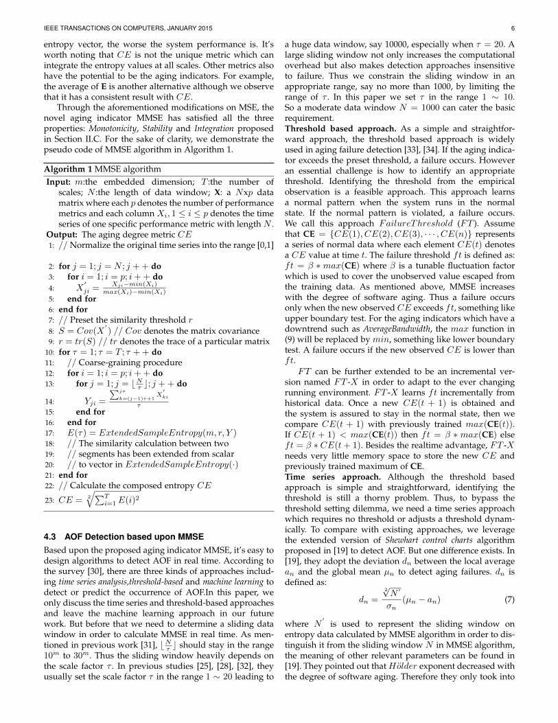
Fig. 4. The variation of GCD sorealong with the number of variables

Fig. 5. Training data selection in FTapproach.

as:

Recall =Ntp

Ntp +Nfn, P recision =

NtpNtp +Nfp

where Ntp, Nfn, and Nfp denote the number of truepositives, false negatives, and false positives respectively.It’s worth noting that Ntp, Nfn, Nfp are the aggregatednumbers over 50 experiments respectively. To represent theaccuracy in a single value, F1-measure is leveraged anddefined as:

F1−measure =2 ∗Recall ∗ PrecisionRecall + Precision

ATTF is defined as the time span between the first failurereport and the real failure namely the left boundary ofthe decision window in this paper. In a real-world system,once a failure is detected the system may be rebooted oroffloaded for maintenance. Thus we choose the first failurereport as a reference point. If the first failure report fallsin the decision window, ATTF = 0. A large ATTF maycause excessive system maintenance leading to availabilitydecrease and operation cost increase. Therefore a lowerATTF is preferred.

5.2 Performance Metric Selection

By investigating all the performance metrics, we find thatmany metrics have very similar characteristics like trendmeaning these metrics are highly correlated. Therefore weselect a small subset of metrics which can be used as asurrogate of the full data set without significant informationloss via PCA variable selection presented in Section V.A. Wecalculate the best GCD scores of different variable sets withspecific cardinalities (e.g. k = 3) by the simulated annealingalgorithm. Figure 4 shows the variation of the best GCDsore along with the number of variables. From this figure,we observe that the GCD score doesn’t increase significantlyany more when the number of variables reaches 5. Thereforethese 5 variables are already capable of representing the fulldata set. The 5 variables are Total CPU Utilization, Average-Badwidth, Process IO Operations Per Second , Process VirtualBytes Peak, Jitter respectively. In the following experiments,we will use them to evaluate CHAOS.

5.3 AOF Detection

In this section, we will demonstrate the the failure detectionresults of CHAOS. In MMSE algorithm, we set the embed-ded dimension m = 2, the sliding window N = 1000,thenumber of scales T = 10. For the failure detection approach

FT , we need to prepare the training data and determinethe fluctuation factor β first. Due to the lack of prior knowl-edge, the training data selection is full of randomness andblindness. To unify the way of training data selection, weleverage the slice of MMSE data ranging from the systemstart point to the point where 200 time slots away from theright boundary of the decision window as the training data.And leave the left 200 time slots to conduct and compare toFT -X approach. Figure 6 shows an example of training dataselection in one experiment. In this figure, we set the pointin the 800th time slot as the “failure” point. The decisionwindow spans across the range 700 ∼ 800. Thus the dataslice in the range 0 ∼ 500 is selected as the training data.

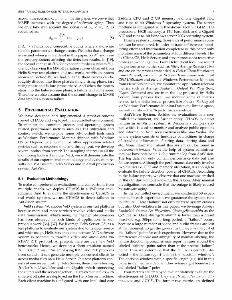
Another problem is how to determine β. According tothe historical performance metrics and failure records, it’spossible to achieve an optimal β. Figure 6 (a) demonstratesthe failure detection results of FT with different β values.From this figure, we observe that Recall keeps a perfectvalue 1 when β varies in the range 1 ∼ 2, i.e. Nfn = 0 andthe other two metrics: Precision and F1-measure increasewith β. From Figure 5, we can find some clues to explainthese observations. In Figure 5, the selected training datain the range 0 ∼ 500 is much smaller than the data inthe decision window. Hence, no matter how β varies in therange 1 ∼ 2, the failure threshold ft is lower than the data inthe decision window. The advantage is that all of the failurescan be pinpointed (i.e. Nfn = 0). While the disadvantage isthat many normal data are mistaken as failures (i.e. Nfp islarge). And the Precision has an increasing trend due tothe decreasing of Nfp with β. Similarly, the detection resultsFT -X with different β values are shown in Figure 6 (b).But quite different from the observations in Figure 6 (a), thePrecision keeps a perfect value 1 (i.e. Nfp = 0) while theother two metrics Recall and F1-measure decrease withβ in Figure 6 (b). Figure 5 is also capable of explainingthese observations. The failure threshold ft is updated byFT -X incrementally according to the system state. As thesystem runs normally in the range 500 ∼ 700, these dataare also used to train ft. Hence max(CE) calculated by FT -X is much bigger than the one calculated by FT . A biggerβ can guarantee the detected failures are the real failures(i.e. Nfp = 0) but may result in a large failure missingrate (i.e. Nfn is large). From these two figures, we observethat FT achieves an optimal result when β is large, sayβ = 2 but FT -X achieves an optimal result when β issmall, say β = 1.1. To carry out fair comparisons, we setβ = 2 for FT and β = 1.1 for FT -X , namely their optimalresults. However in real-world applications, the optimal βis considerably difficult to attain especially when failurerecords are scarce. In that case, β can be determined by rule-of-thumb.

Although the extended version of Shewhart control chartsis capable of identifying failures adaptively, it’s still nec-essary to determine two parameters, namely the slidingwindow N

′and ε in order to obtain an optimal detection

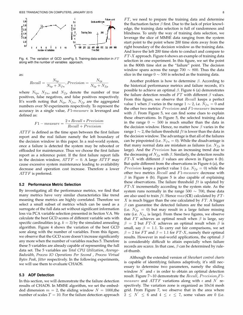
result. Figure 7∼10 demonstrate the Recall, Precision,F1-measure and ATTF variations along with ε and N

′re-

spectively. The variation zone is organized as 10x14 meshgrid. From Figure 7, we observe that in the area where2 ≤ N

′ ≤ 6 and 4 ≤ ε ≤ 7, some values are 0 (i.e.


Fig. 6. The variations of Recall,Precision and F1-measure along withβ values. (a) and (b) demonstrate the variations in FT approach andFT -X approach respectively.

Fig. 7. Recall variations Fig. 8. Precision variations

Fig. 9. F1-measure variations Fig. 10. ATTF variations

Ntp = 0) as there are no deviations exceeding the thresh-old ε. Accordingly, the Precision and F1-measure are 0too. But in other areas, all the failure points are detected(i.e. Recall = 1). Thus F1-measure changes consistentlywith Precision. Here we choose the optimal result whenN = 6 and ε = 6.5 according to F1-measure. At thispoint, Recall = 1,Precision = 0.99, F1-measure=0.995 andATTF = 6.

In the following experiments, we will compare the de-tection results of FT , FT -X and the extended version ofShewhart control charts when they achieve the optimal resultsin the Helix Server system and the real-world AntVisionsystem. In different systems, we will determine the optimalresults for different approaches separately.

Figure 11 depicts the comparisons of the failure detectionresults obtained by FT , FT -X and the extended Shewhartcontrol charts in Helix Sever system. From Figure 11.(a),we observe that the extended version of Shewhart controlchart achieves the best result, F1-measure=0.995; FT -Xachieves the second best result, F1-measure=0.9795; FTachieves the worst result, F1-measure=0.8899. The detec-tion results of the extended Shewhart control chart and FT -Xhave about 0.1 improvement compared to the one of FT .Meanwhile, a lower ATTF is obtained by the adaptiveapproaches such as FT -X , shown in Figure 11.(b). A lowerATTF not only guarantees the failure could be detected in

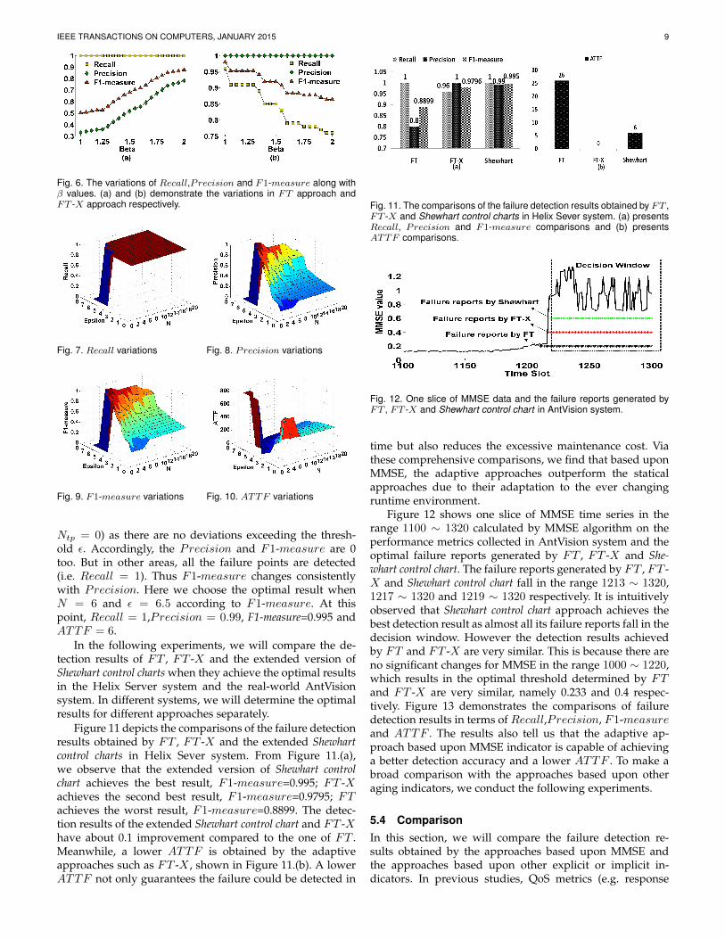
Fig. 11. The comparisons of the failure detection results obtained by FT ,FT -X and Shewhart control charts in Helix Sever system. (a) presentsRecall, Precision and F1-measure comparisons and (b) presentsATTF comparisons.

Fig. 12. One slice of MMSE data and the failure reports generated byFT , FT -X and Shewhart control chart in AntVision system.

time but also reduces the excessive maintenance cost. Viathese comprehensive comparisons, we find that based uponMMSE, the adaptive approaches outperform the staticalapproaches due to their adaptation to the ever changingruntime environment.

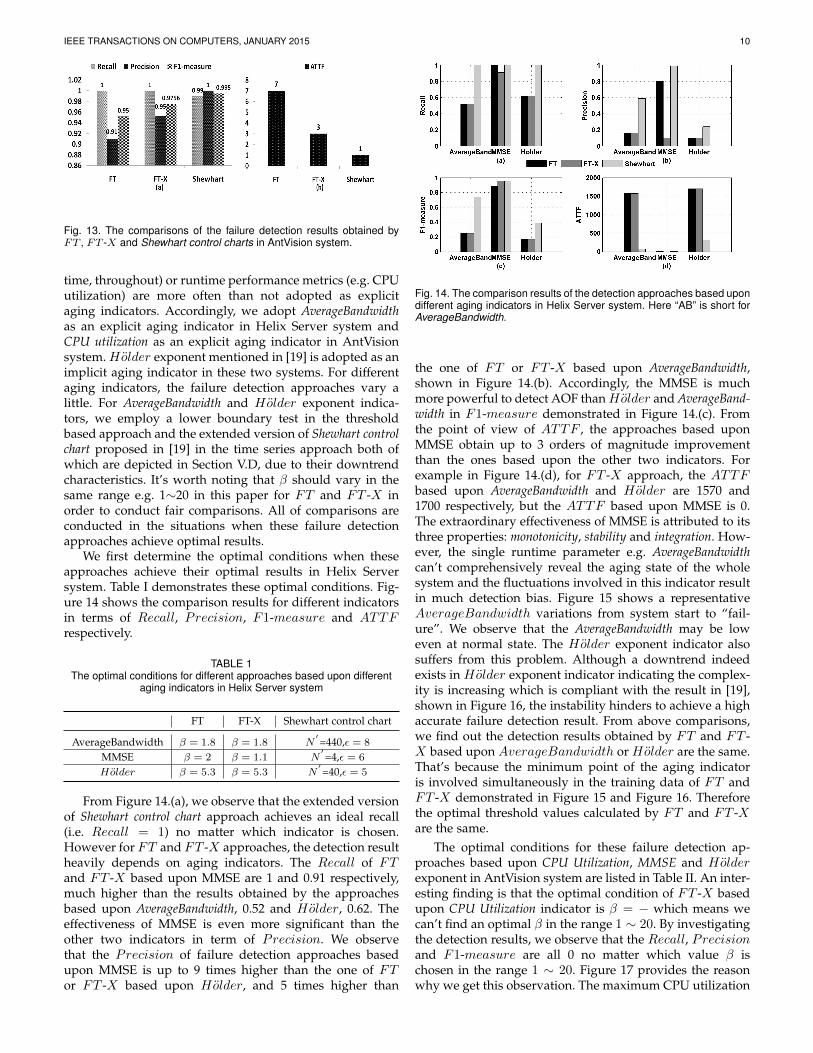
Figure 12 shows one slice of MMSE time series in therange 1100 ∼ 1320 calculated by MMSE algorithm on theperformance metrics collected in AntVision system and theoptimal failure reports generated by FT , FT -X and She-whart control chart. The failure reports generated by FT , FT -X and Shewhart control chart fall in the range 1213 ∼ 1320,1217 ∼ 1320 and 1219 ∼ 1320 respectively. It is intuitivelyobserved that Shewhart control chart approach achieves thebest detection result as almost all its failure reports fall in thedecision window. However the detection results achievedby FT and FT -X are very similar. This is because there areno significant changes for MMSE in the range 1000 ∼ 1220,which results in the optimal threshold determined by FTand FT -X are very similar, namely 0.233 and 0.4 respec-tively. Figure 13 demonstrates the comparisons of failuredetection results in terms of Recall,Precision, F1-measureand ATTF . The results also tell us that the adaptive ap-proach based upon MMSE indicator is capable of achievinga better detection accuracy and a lower ATTF . To make abroad comparison with the approaches based upon otheraging indicators, we conduct the following experiments.

5.4 ComparisonIn this section, we will compare the failure detection re-sults obtained by the approaches based upon MMSE andthe approaches based upon other explicit or implicit in-dicators. In previous studies, QoS metrics (e.g. response


Fig. 13. The comparisons of the failure detection results obtained byFT , FT -X and Shewhart control charts in AntVision system.

time, throughout) or runtime performance metrics (e.g. CPUutilization) are more often than not adopted as explicitaging indicators. Accordingly, we adopt AverageBandwidthas an explicit aging indicator in Helix Server system andCPU utilization as an explicit aging indicator in AntVisionsystem.Holder exponent mentioned in [19] is adopted as animplicit aging indicator in these two systems. For differentaging indicators, the failure detection approaches vary alittle. For AverageBandwidth and Holder exponent indica-tors, we employ a lower boundary test in the thresholdbased approach and the extended version of Shewhart controlchart proposed in [19] in the time series approach both ofwhich are depicted in Section V.D, due to their downtrendcharacteristics. It’s worth noting that β should vary in thesame range e.g. 1∼20 in this paper for FT and FT -X inorder to conduct fair comparisons. All of comparisons areconducted in the situations when these failure detectionapproaches achieve optimal results.

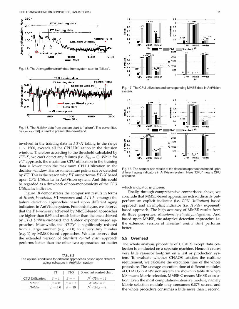
We first determine the optimal conditions when theseapproaches achieve their optimal results in Helix Serversystem. Table I demonstrates these optimal conditions. Fig-ure 14 shows the comparison results for different indicatorsin terms of Recall, Precision, F1-measure and ATTFrespectively.

TABLE 1The optimal conditions for different approaches based upon different

aging indicators in Helix Server system

FT FT-X Shewhart control chart

AverageBandwidth β = 1.8 β = 1.8 N′=440,ε = 8

MMSE β = 2 β = 1.1 N′=4,ε = 6

Holder β = 5.3 β = 5.3 N′=40,ε = 5

From Figure 14.(a), we observe that the extended versionof Shewhart control chart approach achieves an ideal recall(i.e. Recall = 1) no matter which indicator is chosen.However for FT and FT -X approaches, the detection resultheavily depends on aging indicators. The Recall of FTand FT -X based upon MMSE are 1 and 0.91 respectively,much higher than the results obtained by the approachesbased upon AverageBandwidth, 0.52 and Holder, 0.62. Theeffectiveness of MMSE is even more significant than theother two indicators in term of Precision. We observethat the Precision of failure detection approaches basedupon MMSE is up to 9 times higher than the one of FTor FT -X based upon Holder, and 5 times higher than

Fig. 14. The comparison results of the detection approaches based upondifferent aging indicators in Helix Server system. Here “AB” is short forAverageBandwidth.

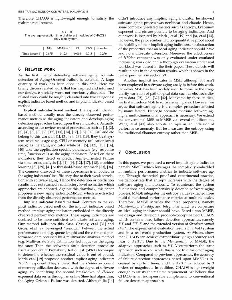
the one of FT or FT -X based upon AverageBandwidth,shown in Figure 14.(b). Accordingly, the MMSE is muchmore powerful to detect AOF thanHolder and AverageBand-width in F1-measure demonstrated in Figure 14.(c). Fromthe point of view of ATTF , the approaches based uponMMSE obtain up to 3 orders of magnitude improvementthan the ones based upon the other two indicators. Forexample in Figure 14.(d), for FT -X approach, the ATTFbased upon AverageBandwidth and Holder are 1570 and1700 respectively, but the ATTF based upon MMSE is 0.The extraordinary effectiveness of MMSE is attributed to itsthree properties: monotonicity, stability and integration. How-ever, the single runtime parameter e.g. AverageBandwidthcan’t comprehensively reveal the aging state of the wholesystem and the fluctuations involved in this indicator resultin much detection bias. Figure 15 shows a representativeAverageBandwidth variations from system start to “fail-ure”. We observe that the AverageBandwidth may be loweven at normal state. The Holder exponent indicator alsosuffers from this problem. Although a downtrend indeedexists in Holder exponent indicator indicating the complex-ity is increasing which is compliant with the result in [19],shown in Figure 16, the instability hinders to achieve a highaccurate failure detection result. From above comparisons,we find out the detection results obtained by FT and FT -X based upon AverageBandwidth or Holder are the same.That’s because the minimum point of the aging indicatoris involved simultaneously in the training data of FT andFT -X demonstrated in Figure 15 and Figure 16. Thereforethe optimal threshold values calculated by FT and FT -Xare the same.

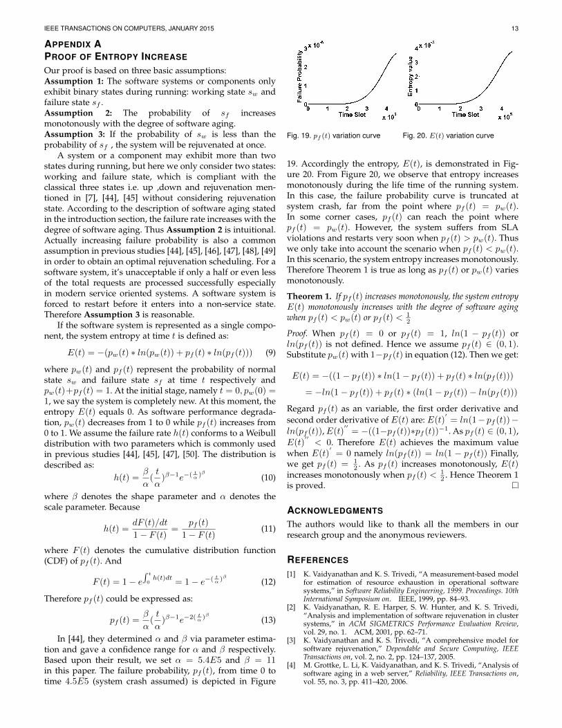
The optimal conditions for these failure detection ap-proaches based upon CPU Utilization, MMSE and Holderexponent in AntVision system are listed in Table II. An inter-esting finding is that the optimal condition of FT -X basedupon CPU Utilization indicator is β = − which means wecan’t find an optimal β in the range 1 ∼ 20. By investigatingthe detection results, we observe that the Recall, Precisionand F1-measure are all 0 no matter which value β ischosen in the range 1 ∼ 20. Figure 17 provides the reasonwhy we get this observation. The maximum CPU utilization


Fig. 15. The AverageBandwidth data from system start to “failure”.

Fig. 16. The Holder data from system start to “failure”. The curve fittedby Lowess [36] is used to present the downtrend.

involved in the training data in FT -X falling in the range1 ∼ 1200, exceeds all the CPU Utilization in the decisionwindow. Therefore according to the threshold calculated byFT -X , we can’t detect any failures (i.e. Ntp = 0). While forFT approach, the maximum CPU utilization in the trainingdata is lower than the maximum CPU Utilization in thedecision window. Hence some failure points can be detectedby FT . This is the reason why FT outperforms FT -X basedupon CPU Utilization in AntVision system. And this couldbe regarded as a drawback of non-monotonicity of the CPUUtilization indicator.

Figure 18 demonstrates the comparison results in termsof Recall,Precision,F1-measure and ATTF amongst thefailure detection approaches based upon different agingindicators in AntVision system. From this figure, we observethat the F1-measure achieved by MMSE-based approachesare higher than 0.95 and much better than the one achievedby CPU Utilization-based and Holder exponent-based ap-proaches. Meanwhile, the ATTF is significantly reducedfrom a large number (e.g. 2300) to a very tiny number(e.g. 1) by MMSE-based approaches. We also observe thatthe extended version of Shewhart control chart approachperforms better than the other two approaches no matter

TABLE 2The optimal conditions for different approaches based upon different

aging indicators in AntVision system

FT FT-X Shewhart control chart

CPU Utilization β = 1 β = − N′=75,ε = 17

MMSE β = 2 β = 1.3 N′=8,ε = 7

Holder β = 4.0 β = 19 N′=165,ε = 8

Fig. 17. The CPU utilization and corresponding MMSE data in AntVisionsystem.

Fig. 18. The comparison results of the detection approaches based upondifferent aging indicators in AntVision system. Here “CPU” means CPUutilization.

which indicator is chosen.Finally, through comprehensive comparisons above, we

conclude that MMSE-based approaches extraordinarily out-perform an explicit indicator (i.e. CPU Utilization) basedapproach and an implicit indicator (i.e. Holder exponent)based approach. The high accuracy of MMSE results fromits three properties: Monotonicity,Stability,Integration. Andbased upon MMSE, the adaptive detection approaches i.e.the extended version of Shewhart control chart performsbetter.

5.5 OverheadThe whole analysis procedure of CHAOS except data col-lection is conducted on a separate machine. Hence it causesvery little resource footprint on a test or production sys-tem. To evaluate whether CHAOS satisfies the realtimerequirement, we calculate the execution time of the wholeprocedure. The average execution time of different modulesof CHAOS in AntVision system are shown in table III whereMS means Metric selection, MMSE-C means MMSE calcula-tion. Even the most computation-intensive module, namelyMetric selection module only consumes 0.875 second andthe whole procedure consumes a little more than 1 second.


Therefore CHAOS is light-weight enough to satisfy therealtime requirement.

TABLE 3The average execution time of different modules of CHAOS in

AntVision system.

MS MMSE-C FT FT-X Shewhart

Time (second) 0.875 0.123 0.016 0.018 0.270

6 RELATED WORK

As the first line of defending software aging, accuratedetection of Aging-Oriented Failure is essential. A largequantity of work has been done in this area. Here webriefly discuss related work that has inspired and informedour design, especially work not previously discussed. Therelated work could be roughly classified into two categories:explicit indicator based method and implicit indicator basedmethod.

Explicit indicator based method: The explicit indicatorbased method usually uses the directly observed perfor-mance metrics as the aging indicators and develops agingdetection approaches based upon these indicators. Actuallyaccording to our review, most of prior studies such as [1], [2],[3], [4], [5], [8], [9], [12], [13], [14], [17], [18], [39], [40] and etcbelong to this class. In [1], [3], [8], [17], [18], they treat sys-tem resource usage (e.g. CPU or memory utilization,swapspace) as the aging indicator while [4], [5], [12], [13], [14],[40] take the application specific parameters (e.g. responsetime, function call) as the aging indicators. Based on theseindicators, they detect or predict Aging-Oriented Failurevia time-series analysis [1], [4], [9], [12], [17], [18], machinelearning [5], [39], [41] or threshold-based approach [33], [34].The common drawback of these approaches is embodied inthe aging indicators’ insufficiency due to their weak correla-tion with software aging. Hence the detection or predictionresults have not reached a satisfactory level no matter whichapproaches are adopted. Against this drawback, this paperproposes a new aging indicator,MMSE, which is extractedfrom the directly observed performance metrics.

Implicit indicator based method: Contrary to the ex-plicit indicator based method, the implicit indicator basedmethod employs aging indicators embedded in the directlyobserved performance metrics. These aging indicators aredeclared to be more sufficient to indicate software aging.Our method falls into this class. Cassidy, et.al [31] andGross, et.al [27] leveraged “residual” between the actualperformance data (e.g. queue length) and the estimated per-formance data obtained by a multivariate analysis method(e.g. Multivariate State Estimation Technique) as the agingindicator. Then the software’s fault detection procedureused a Sequential Probability Ratio Test (SPRT) techniqueto determine whether the residual value is out of bound.Mark, et.al [19] proposed another implicit aging indicator:Holder exponent. They showed that the Holder exponentof memory utilization decreased with the degree of softwareaging. By identifying the second breakdown of Holderexponent data series through an online Shewhart algorithm,the Aging-Oriented Failure was detected. Although Jia [14]

didn’t introduce any implicit aging indicator, he showedsoftware aging process was nonlinear and chaotic. Hence,some complexity-related metrics such as entropy, Lyapunovexponent and etc are possible to be aging indicators. Andour work is inspired by Mark , et.al [19] and Jia, et.al [14].However, the prior studies had no quantitative proof aboutthe viability of their implicit aging indicators, no abstractionof the properties that an ideal aging indicator should haveand no multi-scale extension. Moreover the effectivenessof Holder exponent was only evaluated under emulatedincreasing workload and a thorough evaluation under realworkload was absent in the their paper. These defects willresult in bias in the detection results, which is shown in thereal experiments in section VI.

Another implicit indicator is MSE, although it hasn’tbeen employed in software aging analysis before this work.However MSE has been widely used to measure the irreg-ularity variation of pathological data such as electrocardio-gram data [25], [28], [32], [42]. Motivated by these studies,we first introduce MSE to software aging area. However, weargue that software aging is a complex procedure affectedby many factors. Hence,to accurate measure software ag-ing, a multi-dimensional approach is necessary. We extendthe conventional MSE to MMSE via several modifications.Wang, et.al [43] also adopts entropy as an indicator ofperformance anomaly. But he measures the entropy usingthe traditional Shannon entropy rather than MSE.

7 CONCLUSION

In this paper, we proposed a novel implicit aging indicatornamely MMSE which leverages the complexity embeddedin runtime performance metrics to indicate software ag-ing. Through theoretical proof and experimental practice,we demonstrate that entropy increases with the degree ofsoftware aging monotonously. To counteract the systemfluctuations and comprehensively describe software agingprocess, MMSE integrates the entropy values extracted frommulti-dimensional performance metrics at multiple scales.Therefore, MMSE satisfies the three properties, namelyMonotonicity, Stability, and Integration which we conjecturean ideal aging indicator should have. Based upon MMSE,we design and develop a proof-of-concept named CHAOSwhich contains three failure detection approaches, namelyFT and FT -X and the extended version of Shewhart controlchart. The experimental evaluation results in a VoD systemand in a real-world production system, AntVision, showthat CHAOS can achieve extraordinarily high accuracy andnear 0 ATTF . Due to the Monotonicity of MMSE, theadaptive approaches such as FT -X outperform the staticapproach such as FT while this is not true for other agingindicators. Compared to previous approaches, the accuracyof failure detection approaches based upon MMSE is in-creased by up to 5 times, and the ATTF is reduced by 3orders of magnitude. In addition, CHAOS is light-weightenough to satisfy the realtime requirement. We believe thatCHAOS is an indispensable complement to conventionalfailure detection approaches.


APPENDIX APROOF OF ENTROPY INCREASE

Our proof is based on three basic assumptions:Assumption 1: The software systems or components onlyexhibit binary states during running: working state sw andfailure state sf .Assumption 2: The probability of sf increasesmonotonously with the degree of software aging.Assumption 3: If the probability of sw is less than theprobability of sf , the system will be rejuvenated at once.

A system or a component may exhibit more than twostates during running, but here we only consider two states:working and failure state, which is compliant with theclassical three states i.e. up ,down and rejuvenation men-tioned in [7], [44], [45] without considering rejuvenationstate. According to the description of software aging statedin the introduction section, the failure rate increases with thedegree of software aging. Thus Assumption 2 is intuitional.Actually increasing failure probability is also a commonassumption in previous studies [44], [45], [46], [47], [48], [49]in order to obtain an optimal rejuvenation scheduling. For asoftware system, it’s unacceptable if only a half or even lessof the total requests are processed successfully especiallyin modern service oriented systems. A software system isforced to restart before it enters into a non-service state.Therefore Assumption 3 is reasonable.

If the software system is represented as a single compo-nent, the system entropy at time t is defined as:

E(t) = −(pw(t) ∗ ln(pw(t)) + pf (t) ∗ ln(pf (t))) (9)

where pw(t) and pf (t) represent the probability of normalstate sw and failure state sf at time t respectively andpw(t)+pf (t) = 1. At the initial stage, namely t = 0, pw(0) =1, we say the system is completely new. At this moment, theentropy E(t) equals 0. As software performance degrada-tion, pw(t) decreases from 1 to 0 while pf (t) increases from0 to 1. We assume the failure rate h(t) conforms to a Weibulldistribution with two parameters which is commonly usedin previous studies [44], [45], [47], [50]. The distribution isdescribed as:

h(t) =β

α(t

α)β−1e−( tα )β (10)

where β denotes the shape parameter and α denotes thescale parameter. Because

h(t) =dF (t)/dt

1− F (t)=

pf (t)

1− F (t)(11)

where F (t) denotes the cumulative distribution function(CDF) of pf (t). And

F (t) = 1− e∫ t0h(t)dt

= 1− e−( tα )β (12)

Therefore pf (t) could be expressed as:

pf (t) =β

α(t

α)β−1e−2( tα )β (13)

In [44], they determined α and β via parameter estima-tion and gave a confidence range for α and β respectively.Based upon their result, we set α = 5.4E5 and β = 11in this paper. The failure probability, pf (t), from time 0 totime 4.5E5 (system crash assumed) is depicted in Figure

Fig. 19. pf (t) variation curve Fig. 20. E(t) variation curve

19. Accordingly the entropy, E(t), is demonstrated in Fig-ure 20. From Figure 20, we observe that entropy increasesmonotonously during the life time of the running system.In this case, the failure probability curve is truncated atsystem crash, far from the point where pf (t) = pw(t).In some corner cases, pf (t) can reach the point wherepf (t) = pw(t). However, the system suffers from SLAviolations and restarts very soon when pf (t) > pw(t). Thuswe only take into account the scenario when pf (t) < pw(t).In this scenario, the system entropy increases monotonously.Therefore Theorem 1 is true as long as pf (t) or pw(t) variesmonotonously.

Theorem 1. If pf (t) increases monotonously, the system entropyE(t) monotonously increases with the degree of software agingwhen pf (t) < pw(t) or pf (t) < 1

2

Proof. When pf (t) = 0 or pf (t) = 1, ln(1 − pf (t)) orln(pf (t)) is not defined. Hence we assume pf (t) ∈ (0, 1).Substitute pw(t) with 1−pf (t) in equation (12). Then we get:

E(t) = −((1− pf (t)) ∗ ln(1− pf (t)) + pf (t) ∗ ln(pf (t)))

= −ln(1− pf (t)) + pf (t) ∗ (ln(1− pf (t))− ln(pf (t)))

Regard pf (t) as an variable, the first order derivative andsecond order derivative of E(t) are: E(t)

′= ln(1− pf (t))−

ln(pf (t)),E(t)′′

= −((1−pf (t))∗pf (t))−1. As pf (t) ∈ (0, 1),E(t)

′′< 0. Therefore E(t) achieves the maximum value

when E(t)′

= 0 namely ln(pf (t)) = ln(1 − pf (t)) Finally,we get pf (t) = 1

2 . As pf (t) increases monotonously, E(t)increases monotonously when pf (t) < 1

2 . Hence Theorem 1is proved.

ACKNOWLEDGMENTS

The authors would like to thank all the members in ourresearch group and the anonymous reviewers.

REFERENCES

[1] K. Vaidyanathan and K. S. Trivedi, “A measurement-based modelfor estimation of resource exhaustion in operational softwaresystems,” in Software Reliability Engineering, 1999. Proceedings. 10thInternational Symposium on. IEEE, 1999, pp. 84–93.

[2] K. Vaidyanathan, R. E. Harper, S. W. Hunter, and K. S. Trivedi,“Analysis and implementation of software rejuvenation in clustersystems,” in ACM SIGMETRICS Performance Evaluation Review,vol. 29, no. 1. ACM, 2001, pp. 62–71.

[3] K. Vaidyanathan and K. S. Trivedi, “A comprehensive model forsoftware rejuvenation,” Dependable and Secure Computing, IEEETransactions on, vol. 2, no. 2, pp. 124–137, 2005.

[4] M. Grottke, L. Li, K. Vaidyanathan, and K. S. Trivedi, “Analysis ofsoftware aging in a web server,” Reliability, IEEE Transactions on,vol. 55, no. 3, pp. 411–420, 2006.


[5] J. Alonso, J. Torres, J. L. Berral, and R. Gavalda, “Adaptive on-line software aging prediction based on machine learning,” in De-pendable Systems and Networks (DSN), 2010 IEEE/IFIP InternationalConference on. IEEE, 2010, pp. 507–516.

[6] S. P. Kavulya, S. Daniels, K. Joshi, M. Hiltunen, R. Gandhi, andP. Narasimhan, “Draco: Statistical diagnosis of chronic problemsin large distributed systems,” in Dependable Systems and Networks(DSN), 2012 42nd Annual IEEE/IFIP International Conference on.IEEE, 2012, pp. 1–12.

[7] Y. Huang, C. Kintala, N. Kolettis, and N. D. Fulton, “Softwarerejuvenation: Analysis, module and applications,” in Fault-TolerantComputing, 1995. FTCS-25. Digest of Papers., Twenty-Fifth Interna-tional Symposium on. IEEE, 1995, pp. 381–390.

[8] J. Araujo, R. Matos, V. Alves, P. Maciel, F. Souza, K. S. Trivedi et al.,“Software aging in the eucalyptus cloud computing infrastructure:Characterization and rejuvenation,” ACM Journal on EmergingTechnologies in Computing Systems (JETC), vol. 10, no. 1, p. 11, 2014.

[9] J. Araujo, R. Matos, P. Maciel, R. Matias, and I. Beicker, “Exper-imental evaluation of software aging effects on the eucalyptuscloud computing infrastructure,” in Proceedings of the Middleware2011 Industry Track Workshop. ACM, 2011, p. 4.

[10] K. Kourai and S. Chiba, “Fast software rejuvenation of virtualmachine monitors,” Dependable and Secure Computing, IEEE Trans-actions on, vol. 8, no. 6, pp. 839–851, 2011.

[11] ——, “A fast rejuvenation technique for server consolidationwith virtual machines,” in Dependable Systems and Networks, 2007.DSN’07. 37th Annual IEEE/IFIP International Conference on. IEEE,2007, pp. 245–255.

[12] D. Cotroneo, R. Natella, R. Pietrantuono, and S. Russo, “Softwareaging analysis of the linux operating system,” in Software ReliabilityEngineering (ISSRE), 2010 IEEE 21st International Symposium on.IEEE, 2010, pp. 71–80.

[13] D. Cotroneo, S. Orlando, and S. Russo, “Characterizing agingphenomena of the java virtual machine,” in Reliable DistributedSystems, 2007. SRDS 2007. 26th IEEE International Symposium on.IEEE, 2007, pp. 127–136.

[14] Y.-F. Jia, L. Zhao, and K.-Y. Cai, “A nonlinear approach to mod-eling of software aging in a web server,” in Software EngineeringConference, 2008. APSEC’08. 15th Asia-Pacific. IEEE, 2008, pp. 77–84.

[15] B. Sharma, P. Jayachandran, A. Verma, and C. R. Das, “Cloudpd:Problem determination and diagnosis in shared dynamic clouds,”in IEEE DSN, 2013.

[16] V. Castelli, R. E. Harper, P. Heidelberger, S. W. Hunter, K. S.Trivedi, K. Vaidyanathan, and W. P. Zeggert, “Proactive manage-ment of software aging,” IBM Journal of Research and Development,vol. 45, no. 2, pp. 311–332, 2001.

[17] P. Zheng, Y. Qi, Y. Zhou, P. Chen, J. Zhan, and M. Lyu, “An au-tomatic framework for detecting and characterizing performancedegradation of software systems,” Reliability, IEEE Transactions on,vol. 63, no. 4, pp. 927–943, 2014.

[18] S. Garg, A. van Moorsel, K. Vaidyanathan, and K. S. Trivedi, “Amethodology for detection and estimation of software aging,” inSoftware Reliability Engineering, 1998. Proceedings. The Ninth Inter-national Symposium on. IEEE, 1998, pp. 283–292.

[19] M. Shereshevsky, J. Crowell, B. Cukic, V. Gandikota, and Y. Liu,“Software aging and multifractality of memory resources,” in2003 33rd Annual IEEE/IFIP International Conference on DependableSystems and Networks (DSN). IEEE Computer Society, 2003, pp.721–730.

[20] I. Jolliffe, Principal component analysis. Wiley Online Library, 2005.[21] J. F. Cadima and I. T. Jolliffe, “Variable selection and the interpre-

tation of principal subspaces,” Journal of agricultural, biological, andenvironmental statistics, vol. 6, no. 1, pp. 62–79, 2001.

[22] J. Ramsay, J. ten Berge, and G. Styan, “Matrix correlation,” Psy-chometrika, vol. 49, no. 3, pp. 403–423, 1984.

[23] J. Cadima, J. O. Cerdeira, and M. Minhoto, “Computational as-pects of algorithms for variable selection in the context of principalcomponents,” Computational statistics & data analysis, vol. 47, no. 2,pp. 225–236, 2004.

[24] C. E. Shannon, “Bell system tech. j. 27 (1948) 379; ce shannon,” BellSystem Tech. J, vol. 27, p. 623, 1948.

[25] M. Costa, A. L. Goldberger, and C.-K. Peng, “Multiscale entropyanalysis of biological signals,” Physical Review E, vol. 71, no. 2, p.021906, 2005.

[26] S. M. Pincus and A. L. Goldberger, “Physiological time-seriesanalysis: what does regularity quantify?” American Journal of Phys-iology, vol. 266, pp. H1643–H1643, 1994.

[27] K. C. Gross, V. Bhardwaj, and R. Bickford, “Proactive detection ofsoftware aging mechanisms in performance critical computers,”in Software Engineering Workshop, 2002. Proceedings. 27th AnnualNASA Goddard/IEEE. IEEE, 2002, pp. 17–23.

[28] M. U. Ahmed and D. P. Mandic, “Multivariate multiscale entropy:A tool for complexity analysis of multichannel data,” PhysicalReview E, vol. 84, no. 6, p. 061918, 2011.

[29] L. Cao, A. Mees, and K. Judd, “Dynamics from multivariate timeseries,” Physica D: Nonlinear Phenomena, vol. 121, no. 1, pp. 75–88,1998.

[30] D. Cotroneo, R. Natella, R. Pietrantuono, and S. Russo, “A surveyof software aging and rejuvenation studies,” ACM Journal onEmerging Technologies in Computing Systems (JETC), vol. 10, no. 1,p. 8, 2014.

[31] K. J. Cassidy, K. C. Gross, and A. Malekpour, “Advanced patternrecognition for detection of complex software aging phenomena inonline transaction processing servers,” in Dependable Systems andNetworks, 2002. DSN 2002. Proceedings. International Conference on.IEEE, 2002, pp. 478–482.

[32] M. Costa, A. L. Goldberger, and C.-K. Peng, “Multiscale entropyanalysis of complex physiologic time series,” Physical review letters,vol. 89, no. 6, p. 068102, 2002.

[33] L. M. Silva, J. Alonso, and J. Torres, “Using virtualization toimprove software rejuvenation,” IEEE Transactions on Computers,vol. 58, no. 11, pp. 1525–1538, 2009.

[34] J. Alonso, I. Goiri, J. Guitart, R. Gavalda, and J. Torres, “Optimalresource allocation in a virtualized software aging platform withsoftware rejuvenation,” in Software Reliability Engineering (ISSRE),2011 IEEE 22nd International Symposium on. IEEE, 2011, pp. 250–259.

[35] [Online]. Available: http://www.sourceforge.net/projects/hyperic-hq

[36] P. Chen, Y. Qi, P. Zheng, J. Zhan, and Y. Wu, “Multi-scale entropy:One metric of software aging,” in Service Oriented System Engineer-ing (SOSE), 2013 IEEE 7th International Symposium on. IEEE, 2013,pp. 162–169.

[37] P. Zheng, Y. Zhou, M. R. Lyu, and Y. Qi, “Granger causality-awareprediction and diagnosis of software degradation,” in ServicesComputing (SCC), 2014 IEEE International Conference on. IEEE,2014, pp. 528–535.

[38] [Online]. Available: http://www.helix-server.helixcommunity.org/

[39] A. Andrzejak and L. Silva, “Using machine learning for non-intrusive modeling and prediction of software aging,” in NetworkOperations and Management Symposium, 2008. NOMS 2008. IEEE.IEEE, 2008, pp. 25–32.

[40] R. Matias, P. A. Barbetta, K. S. Trivedi et al., “Accelerated degrada-tion tests applied to software aging experiments,” Reliability, IEEETransactions on, vol. 59, no. 1, pp. 102–114, 2010.

[41] J. P. Magalhaes and L. Moura Silva, “Prediction of performanceanomalies in web-applications based-on software aging scenar-ios,” in Software Aging and Rejuvenation (WoSAR), 2010 IEEE SecondInternational Workshop on. IEEE, 2010, pp. 1–7.

[42] M. U. Ahmed and D. P. Mandic, “Multivariate multiscale entropyanalysis,” Signal Processing Letters, IEEE, vol. 19, no. 2, pp. 91–94,2012.

[43] C. Wang, V. Talwar, K. Schwan, and P. Ranganathan, “Onlinedetection of utility cloud anomalies using metric distributions,”in Network Operations and Management Symposium (NOMS), 2010IEEE. IEEE, 2010, pp. 96–103.

[44] J. Zhao, Y. Jin, K. S. Trivedi, and R. Matias, “Injecting memory leaksto accelerate software failures,” in Software Reliability Engineering(ISSRE), 2011 IEEE 22nd International Symposium on. IEEE, 2011,pp. 260–269.

[45] K. S. Trivedi, K. Vaidyanathan, and K. Goseva-Popstojanova,“Modeling and analysis of software aging and rejuvenation,” inSimulation Symposium, 2000.(SS 2000) Proceedings. 33rd Annual.IEEE, 2000, pp. 270–279.

[46] A. Bobbio, M. Sereno, and C. Anglano, “Fine grained softwaredegradation models for optimal rejuvenation policies,” Perfor-mance Evaluation, vol. 46, no. 1, pp. 45–62, 2001.

[47] Y. Bao, X. Sun, and K. S. Trivedi, “A workload-based analysis ofsoftware aging, and rejuvenation,” Reliability, IEEE Transactions on,vol. 54, no. 3, pp. 541–548, 2005.

http://www.sourceforge.net/projects/hyperic-hq

http://www.sourceforge.net/projects/hyperic-hq

http://www.helix-server.helixcommunity.org/

http://www.helix-server.helixcommunity.org/


[48] T. Dohi, K. Goseva-Popstojanova, and K. S. Trivedi, “Analysisof software cost models with rejuvenation,” in High AssuranceSystems Engineering, 2000, Fifth IEEE International Symposim on.HASE 2000. IEEE, 2000, pp. 25–34.

[49] R. E. Barlow and R. A. Campo, “Total time on test processes andapplications to failure data analysis.” DTIC Document, Tech. Rep.,1975.

[50] T. Dohi, K. Goseva-Popstojanova, and K. S. Trivedi, “Statisticalnon-parametric algorithms to estimate the optimal software re-juvenation schedule,” in Dependable Computing, 2000. Proceedings.2000 Pacific Rim International Symposium on. IEEE, 2000, pp. 77–84.

Documents

IEEE TRANSACTIONS ON COMPUTERS, JANUARY … (e.g. software bugs) and external (e.g. resource exhaustion) impairments. These chronic problems often ﬂy under the radar of software