IEEE TRANSACTIONS ON GEOSCIENCE AND REMOTE SENSING 1

Impact of scene decorrelation on GeosynchronousSAR data focusing

Andrea Recchia, Andrea Monti Guarnieri, Member, IEEE, Antoni Broquetas, Member, IEEE, Antonio Leanza

Abstract—We discuss the effects of the clutter on Geosyn-chronous SAR systems exploiting long integration times (fromminutes to hours) to counteract for 2-way propagation losses andincrease azimuth resolution. Only stable targets will be correctlyfocused whereas unstable targets will spread their energy alongazimuth direction. We derive here a generic model for thespreading of the clutter energy based on the power spectraldensity of the clutter itself. We then assume the BillingsleyIntrinsic Clutter Motion model, representing the clutter powerspectrum as an exponential decay, and derive the expectedGEOSAR Signal-to-Clutter Ratio. We also provide some resultsfrom a Ground Based RADAR experiment aimed at assessing thelong term clutter statistics for different scenarios to complementthe ICM model, mainly derived for windblown trees. Finally wediscuss the expected performances of two GEOSAR systems withdifferent acquisition geometries.

I. INTRODUCTION

A Synthetic Aperture Radar placed in geosynchronous orbit(GEOSAR) was first proposed at the end of the seventies [1][2]. Since then, several GEOSAR systems have been proposedbut never implemented due to both technological constraints[3] and the presence of decorrelation sources impacting on thequality of the focused images [4]. Nevertheless the growinginterest in GEOSAR systems is justified by their potentialapplications. In particular the daily revisit could enable thenear real time monitoring of geophysical phenomena with timescales much faster than those currently observed with LowEarth Orbit SAR (LEOSAR) constellations.

GEOSAR systems exploit long integration times to increaseresolution and compensate spread losses, making the sceneresponse during the dwell time non stable. From one sidethe Atmospheric Phase Screen (APS), if not properly com-pensated, could prevent data focusing when integration timeextends from several minutes to hours [5]–[7]. On the otherhand the response of the targets itself can change during thedwell time. The energy of non stable targets, after focusing,will spread along azimuth direction affecting the Signal-to-Clutter Ratio (SCR) even for very stable targets such as urbanand rocky areas [4].

In the present paper we neglect atmospheric effects andconcentrate on the impact of the clutter decorrelation on aGEOSAR system. For short integration time SAR systems(< 1 s) the clutter is assumed stationary within the dwelltime and, after focusing, impairs the detection of the targetsof interest. Unlike thermal noise, the Signal-to-Clutter Ratio

A. Recchia, A. Monti Guarnieri and A. Leanza are with the Dipartimentodi Elettronica, Informazione e Bioingegneria, Politecnico di Milano, Milano,via Ponzio 34, 20133, e-mail: andrea.recchia@aresys.it.

A. Broquetas is with Universitat Politecnica de Catalunya.

cannot be improved by increasing the transmitted power butonly enhancing the system resolution. Ulaby and Dobsonexperimentally derived models for the characterization of theclutter in terms of Normalized Radar Cross Section (σ0) fordifferent classes of terrain at different grazing angles [8].

The increase of the integration time and the reduction ofthe wavelength in modern SAR systems, aimed at improvingresolution like in Spotlight SAR [9], pose the problem ofnon stationary clutter, which also affects applications likeMoving Target Indication [10], [11]. For this reason, nonstationary clutter has been widely investigated by Billingsley,who introduced the Internal Clutter Motion (ICM) model,experimentally derived for windblown trees at different bands(from L to X) [12]. The ICM model is a good approximationof the non stationary clutter spectrum for observation times upto 1 minute. The validity of the ICM model has never beenproven for longer observation times like those exploited by aGEOSAR system, which can extend to hours [13] [14].

The aim of this paper is twofold. On one hand we introducea theoretical model for the evaluation of the expected SCRin a generic GEOSAR system. The SCR model explicitlyinclude the effects of non stationary clutter, always neglectedfor standard LEOSAR systems. The new performance modelscan be exploited for the design of future GEOSAR missions.On the other hand we provide a preliminary assessment ofthe ICM model validity for long integration times exploitinga set of Ground Based RADAR acquisitions at Ku band. Theanalysis shows that the ICM model is not totally valid forlong integration times, at least in terms of the values of themodel parameters indicated by Billingsley. In any case furtherextensive GB RADAR campaigns should be carried out toprovide a meaningful statistical characterization of the nonstationary clutter over long observation times and for differentclasses of targets.

The paper is organized as follows. In Section II we introducethe GEOSAR concept and define the received and focused sig-nal models. In Section III we provide a statistical descriptionof the non stationary clutter as a Brownian motion, which canbe directly related to the Billingsley ICM model. In Section IVwe derive the theoretical expressions for the SCR in a genericGEOSAR system. Finally in Section V we evaluate the SCRexpressions for two different GEOSAR concepts, assessingtheir robustness in front of the scene decorrelation.

IEEE TRANSACTIONS ON GEOSCIENCE AND REMOTE SENSING 2

II. GEOSAR CONCEPTS AND SIGNAL MODELS

A. GEOSAR concepts

Two main GEOSAR concepts have been proposed in liter-ature. The first one achieves continental coverage by meansof a significant orbit inclination [2]. Integration time in theorder of minutes, high power and quite large antennas areexploited to counteract for the spread losses. According to [3]road-map, such system would require 2020 technologies to beimplemented.

A totally different concept, first proposed in [15], is basedon a negligible orbit inclination, very long integration timesand reduced requirements in terms of power and antenna size,making it suited to be hosted as an additional payload on acommercial telecommunication satellite (TeLecom COMPati-ble concept).

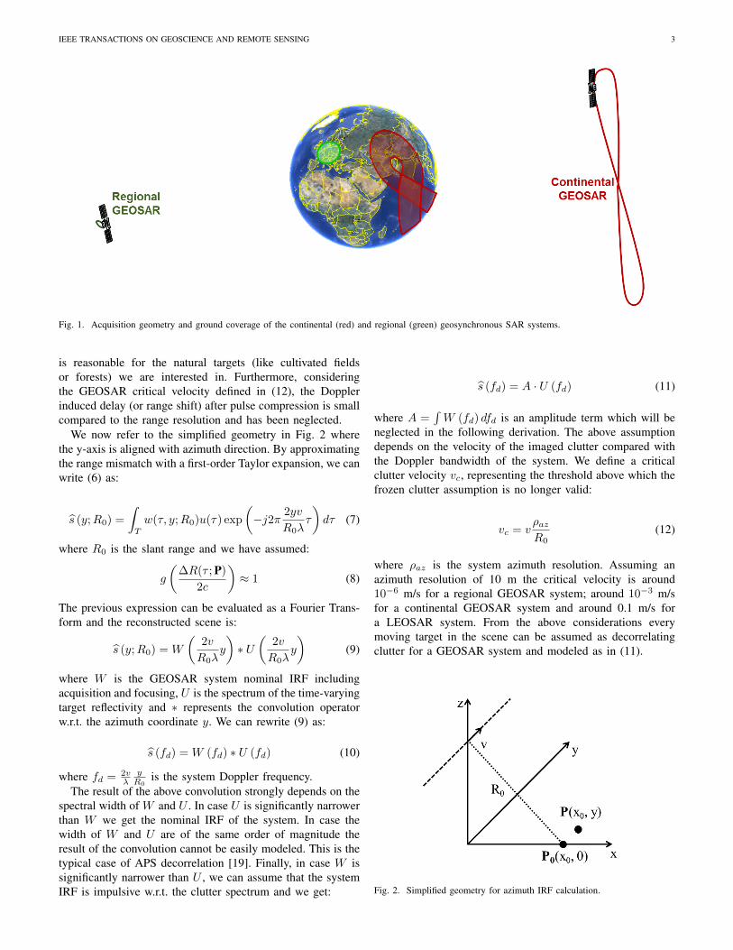
Fig. 1 compares the two GEOSAR concepts in termsof orbit (in an Earth Fixed Reference System) and groundcoverage. The continental system would allow to monitor avery large area - say from Equator to mid latitudes of bothhemispheres - in a non continuous way. On the contrary thereduced orbit extension of the TLCOMP system would allowthe continuous monitoring - say a low resolution image every15 minutes - of a region located at mid latitude such as CentralEurope.

System Continental TLCOMPOrbit Inclination 50 Close to 0

Antennadiameter 15-30 m 1-3 m

AverageTransmitted

Power3000 W 400 W

PRF 200 Hz 50 HzVelocity @

Equator 1100 m/s 5 m/s

Integration time 1-2 minutes 15 minutes - 8 hours

Atmosphere Almost Frozen Sensed - To BeCompensated

Revisit time 24 hours 12 hours

Implementation Dedicated sensorPayload on a DBS

geosynchronoussatellite

TABLE ICOMPARISON BETWEEN MAIN SYSTEM PARAMETERS OF CONTINENTAL

AND TLCOMP SYSTEMS.

Table I provides a comparison between the main systemparameters of the GEOSAR concepts. The values for thecontinental system were retrieved from [2] and [16] whilefor the TLCOMP concept we take as reference the systemproposed in [17]. GEOSAR systems would be the naturalcomplement to standard LEOSAR sensors, providing nearlyreal time monitoring of events such landslides, motion ofglaciers and volcanoes, ground subsidence and building de-formation in urban areas. Furthermore TLCOMP sensitivityto the atmospheric delay could be exploited to generate WaterVapor maps over stable land surfaces, which would providevaluable information to Numerical Weather Prediction models.

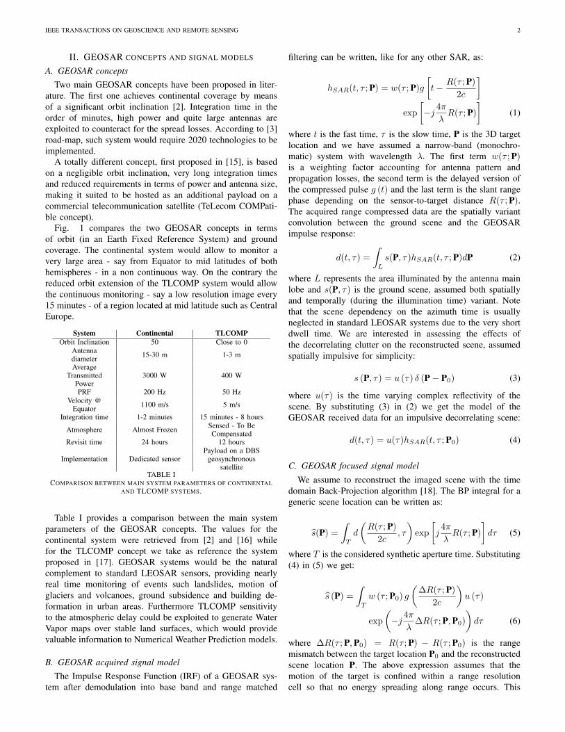
B. GEOSAR acquired signal model

The Impulse Response Function (IRF) of a GEOSAR sys-tem after demodulation into base band and range matched

filtering can be written, like for any other SAR, as:

hSAR(t, τ ; P) = w(τ ; P)g

[t− R(τ ; P)

2c

]exp

[−j 4π

λR(τ ; P)

](1)

where t is the fast time, τ is the slow time, P is the 3D targetlocation and we have assumed a narrow-band (monochro-matic) system with wavelength λ. The first term w(τ ; P)is a weighting factor accounting for antenna pattern andpropagation losses, the second term is the delayed version ofthe compressed pulse g (t) and the last term is the slant rangephase depending on the sensor-to-target distance R(τ ; P).The acquired range compressed data are the spatially variantconvolution between the ground scene and the GEOSARimpulse response:

d(t, τ) =

∫L

s(P, τ)hSAR(t, τ ; P)dP (2)

where L represents the area illuminated by the antenna mainlobe and s(P, τ) is the ground scene, assumed both spatiallyand temporally (during the illumination time) variant. Notethat the scene dependency on the azimuth time is usuallyneglected in standard LEOSAR systems due to the very shortdwell time. We are interested in assessing the effects ofthe decorrelating clutter on the reconstructed scene, assumedspatially impulsive for simplicity:

s (P, τ) = u (τ) δ (P− P0) (3)

where u(τ) is the time varying complex reflectivity of thescene. By substituting (3) in (2) we get the model of theGEOSAR received data for an impulsive decorrelating scene:

d(t, τ) = u(τ)hSAR(t, τ ; P0) (4)

C. GEOSAR focused signal model

We assume to reconstruct the imaged scene with the timedomain Back-Projection algorithm [18]. The BP integral for ageneric scene location can be written as:

s(P) =

∫T

d

(R(τ ; P)

2c, τ

)exp

[j

4π

λR(τ ; P)

]dτ (5)

where T is the considered synthetic aperture time. Substituting(4) in (5) we get:

s (P) =

∫T

w (τ ; P0) g

(∆R(τ ; P)

2c

)u (τ)

exp

(−j 4π

λ∆R(τ ; P,P0)

)dτ (6)

where ∆R(τ ; P,P0) = R(τ ; P) − R(τ ; P0) is the rangemismatch between the target location P0 and the reconstructedscene location P. The above expression assumes that themotion of the target is confined within a range resolutioncell so that no energy spreading along range occurs. This

IEEE TRANSACTIONS ON GEOSCIENCE AND REMOTE SENSING 3

Fig. 1. Acquisition geometry and ground coverage of the continental (red) and regional (green) geosynchronous SAR systems.

is reasonable for the natural targets (like cultivated fieldsor forests) we are interested in. Furthermore, consideringthe GEOSAR critical velocity defined in (12), the Dopplerinduced delay (or range shift) after pulse compression is smallcompared to the range resolution and has been neglected.

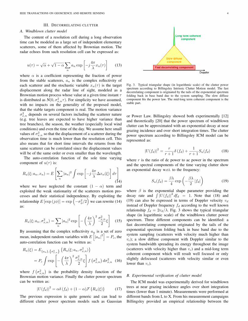
We now refer to the simplified geometry in Fig. 2 wherethe y-axis is aligned with azimuth direction. By approximatingthe range mismatch with a first-order Taylor expansion, we canwrite (6) as:

s (y;R0) =

∫T

w(τ, y;R0)u(τ) exp

(−j2π 2yv

R0λτ

)dτ (7)

where R0 is the slant range and we have assumed:

g

(∆R(τ ; P)

2c

)≈ 1 (8)

The previous expression can be evaluated as a Fourier Trans-form and the reconstructed scene is:

s (y;R0) = W

(2v

R0λy

)∗ U

(2v

R0λy

)(9)

where W is the GEOSAR system nominal IRF includingacquisition and focusing, U is the spectrum of the time-varyingtarget reflectivity and ∗ represents the convolution operatorw.r.t. the azimuth coordinate y. We can rewrite (9) as:

s (fd) = W (fd) ∗ U (fd) (10)

where fd = 2vλ

yR0

is the system Doppler frequency.The result of the above convolution strongly depends on the

spectral width of W and U . In case U is significantly narrowerthan W we get the nominal IRF of the system. In case thewidth of W and U are of the same order of magnitude theresult of the convolution cannot be easily modeled. This is thetypical case of APS decorrelation [19]. Finally, in case W issignificantly narrower than U , we can assume that the systemIRF is impulsive w.r.t. the clutter spectrum and we get:

s (fd) = A · U (fd) (11)

where A =∫W (fd) dfd is an amplitude term which will be

neglected in the following derivation. The above assumptiondepends on the velocity of the imaged clutter compared withthe Doppler bandwidth of the system. We define a criticalclutter velocity vc, representing the threshold above which thefrozen clutter assumption is no longer valid:

vc = vρazR0

(12)

where ρaz is the system azimuth resolution. Assuming anazimuth resolution of 10 m the critical velocity is around10−6 m/s for a regional GEOSAR system; around 10−3 m/sfor a continental GEOSAR system and around 0.1 m/s fora LEOSAR system. From the above considerations everymoving target in the scene can be assumed as decorrelatingclutter for a GEOSAR system and modeled as in (11).

Fig. 2. Simplified geometry for azimuth IRF calculation.

IEEE TRANSACTIONS ON GEOSCIENCE AND REMOTE SENSING 4

III. DECORRELATING CLUTTER

A. Windblown clutter model

The content of a resolution cell during a long observationtime can be modeled as a large set of independent elementaryscatterers, some of them affected by Brownian motion. Theradar echoes from such resolution cell can be expressed as:

u(τ) =√α+√

1− α∑n

an exp

[−j 4π

λxn(τ)

](13)

where α is a coefficient representing the fraction of powerfrom the stable scatterers, an is the complex reflectivity ofeach scatterer and the stochastic variable xn(τ) is the targetdisplacement along the radar line of sight, modeled as aBrownian motion process whose value at a given time instant τis distributed as N(0, σ2

x,nτ). For simplicity we have assumed,with no impacts on the generality of the proposed model,that the stable targets component is real. The motion varianceσ2x,n depends on several factors including the scatterer nature

(e.g. tree leaves are expected to have higher variance thantree branches), the season, the weather (especially local windconditions) and even the time of the day. We assume here smallvalues of σ2

x,n so that the displacement of a scatterer during theobservation time is much lower than the resolution cell. Thisalso means that for short time intervals the returns from thesame scatterer can be correlated since the displacement valueswill be of the same order or even smaller than the wavelength.

The auto-correlation function of the sole time varyingcomponent of u(τ) is:

Ru(ξ; an, xn) = E

[∑n

|an|2∫

exp

[−j 4π

λ∆xn(ξ)

]dτ

](14)

where we have neglected the constant (1 − α) term andexploited the weak stationarity of the scatterers motion pro-cesses and their statistical independence. By exploiting therelationship E [exp (jφ)] = exp

(−σ2

φ/2)

we can rewrite (14)as:

Ru(ξ; an, σ2x,n) =

∑n

|an|2 exp

[−(

4π

λ

)2 σ2x,n

2ξ

](15)

By assuming that the complex reflectivity an is a set of zeromean, independent random variables with E

[|an|2

]= Pc, the

auto-correlation function can be written as:

Ru(ξ) = E{an},{σ2x,n}

{Ru(ξ; an, σ

2x,n)

}= Pc

∫exp

[−(

4π

λ

)2 σ2x,n

2ξ

]f(σ2x,n

)dσ2

x,n (16)

where f(σ2x,n

)is the probability density function of the

Brownian motion variance. Finally the clutter power spectrumcan be written as:

|U(fd)|2 = αδ (fd) + (1− α)F {Ru(ξ)} (17)

The previous expression is quite generic and can lead todifferent clutter power spectrum models such as Gaussian

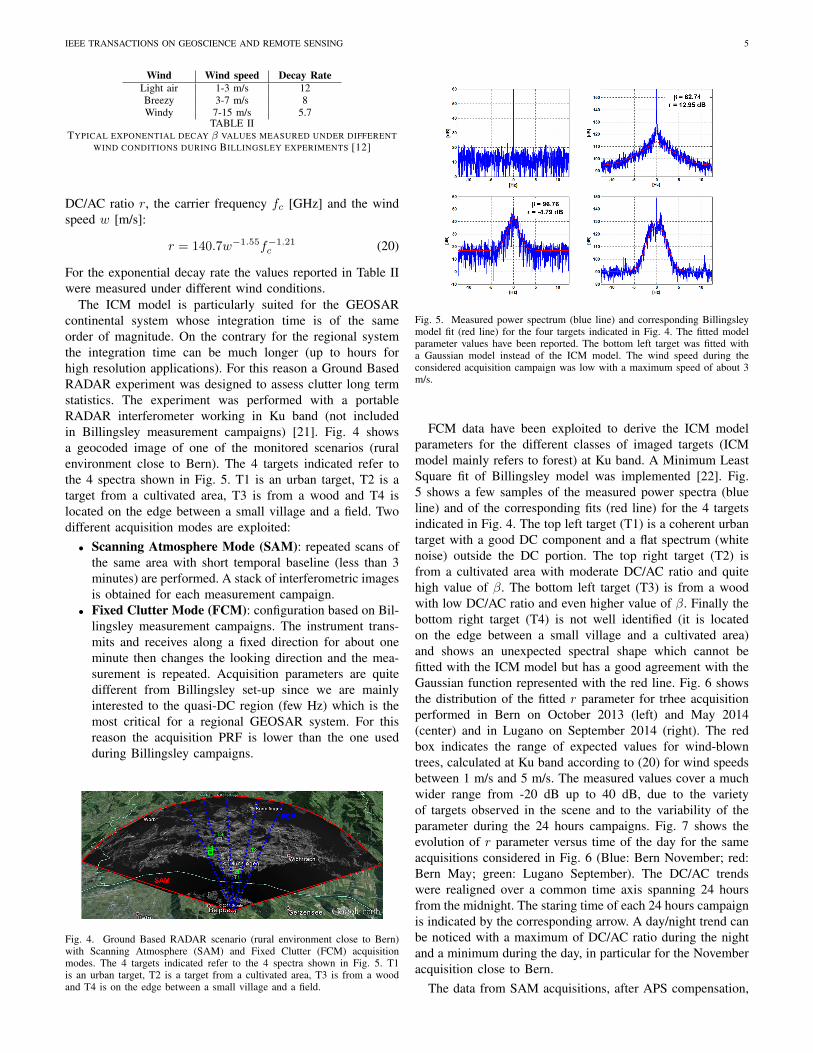
Fig. 3. Typical triangular shape (in logarithmic scale) of the clutter powerspectrum according to Billingsley Intrinsic Clutter Motion model. The fastdecorrelating component is originated by the tails of the exponential spectrumfolding back in base band due to the system sampling. The slow diffusecomponent fits the power law. The mid-long term coherent component is thestable part.

or Power Law. Billingsley showed both experimentally [12]and theoretically [20] that the power spectrum of windblownclutter can be approximated with an exponential decay at neargrazing incidence and over short integration times. The clutterpower spectrum according to Billingsley ICM model can berepresented as:

|U(fd)|2 =r

r + 1δ (fd) +

1

r + 1Su(fd) (18)

where r is the ratio of dc power to ac power in the spectrumand the spectral components of the time varying clutter showan exponential decay w.r.t. to the frequency:

Su(fd) =βλ

4exp

(−βλ

2|fd|)

(19)

where β is the exponential shape parameter providing thedecay rate and

∫|U(fd)|2 dfd = 1. Note that (18) and

(19) can also be expressed in terms of Doppler velocity vdinstead of Doppler frequency fd according to the well knownrelationship fd = 2vd/λ. Fig. 3 shows the typical triangularshape (in logarithmic scale) of the windblown clutter powerspectrum. Three different components can be identified: afast decorrelating component originated by the tails of theexponential spectrum folding back in base band due to thesystem sampling (scatterers with velocity much higher thanvc); a slow diffuse component with Doppler similar to thesystem bandwidth spreading its energy throughout the image(scatterers with velocity higher than vc) and a mid-long termcoherent component which will result well focused or onlyslightly defocused (scatterers with velocity similar or evenlower than vc).

B. Experimental verification of clutter model

The ICM model was experimentally derived for windblowntrees at near grazing incidence angles over short integrationtimes (lower than 1 minute). Measurements were performed atdifferent bands from L to X. From his measurement campaignsBillingsley provided an empirical relationship between the

IEEE TRANSACTIONS ON GEOSCIENCE AND REMOTE SENSING 5

Wind Wind speed Decay RateLight air 1-3 m/s 12Breezy 3-7 m/s 8Windy 7-15 m/s 5.7

TABLE IITYPICAL EXPONENTIAL DECAY β VALUES MEASURED UNDER DIFFERENT

WIND CONDITIONS DURING BILLINGSLEY EXPERIMENTS [12]

DC/AC ratio r, the carrier frequency fc [GHz] and the windspeed w [m/s]:

r = 140.7w−1.55f−1.21c (20)

For the exponential decay rate the values reported in Table IIwere measured under different wind conditions.

The ICM model is particularly suited for the GEOSARcontinental system whose integration time is of the sameorder of magnitude. On the contrary for the regional systemthe integration time can be much longer (up to hours forhigh resolution applications). For this reason a Ground BasedRADAR experiment was designed to assess clutter long termstatistics. The experiment was performed with a portableRADAR interferometer working in Ku band (not includedin Billingsley measurement campaigns) [21]. Fig. 4 showsa geocoded image of one of the monitored scenarios (ruralenvironment close to Bern). The 4 targets indicated refer tothe 4 spectra shown in Fig. 5. T1 is an urban target, T2 is atarget from a cultivated area, T3 is from a wood and T4 islocated on the edge between a small village and a field. Twodifferent acquisition modes are exploited:• Scanning Atmosphere Mode (SAM): repeated scans of

the same area with short temporal baseline (less than 3minutes) are performed. A stack of interferometric imagesis obtained for each measurement campaign.

• Fixed Clutter Mode (FCM): configuration based on Bil-lingsley measurement campaigns. The instrument trans-mits and receives along a fixed direction for about oneminute then changes the looking direction and the mea-surement is repeated. Acquisition parameters are quitedifferent from Billingsley set-up since we are mainlyinterested to the quasi-DC region (few Hz) which is themost critical for a regional GEOSAR system. For thisreason the acquisition PRF is lower than the one usedduring Billingsley campaigns.

Fig. 4. Ground Based RADAR scenario (rural environment close to Bern)with Scanning Atmosphere (SAM) and Fixed Clutter (FCM) acquisitionmodes. The 4 targets indicated refer to the 4 spectra shown in Fig. 5. T1is an urban target, T2 is a target from a cultivated area, T3 is from a woodand T4 is on the edge between a small village and a field.

Fig. 5. Measured power spectrum (blue line) and corresponding Billingsleymodel fit (red line) for the four targets indicated in Fig. 4. The fitted modelparameter values have been reported. The bottom left target was fitted witha Gaussian model instead of the ICM model. The wind speed during theconsidered acquisition campaign was low with a maximum speed of about 3m/s.

FCM data have been exploited to derive the ICM modelparameters for the different classes of imaged targets (ICMmodel mainly refers to forest) at Ku band. A Minimum LeastSquare fit of Billingsley model was implemented [22]. Fig.5 shows a few samples of the measured power spectra (blueline) and of the corresponding fits (red line) for the 4 targetsindicated in Fig. 4. The top left target (T1) is a coherent urbantarget with a good DC component and a flat spectrum (whitenoise) outside the DC portion. The top right target (T2) isfrom a cultivated area with moderate DC/AC ratio and quitehigh value of β. The bottom left target (T3) is from a woodwith low DC/AC ratio and even higher value of β. Finally thebottom right target (T4) is not well identified (it is locatedon the edge between a small village and a cultivated area)and shows an unexpected spectral shape which cannot befitted with the ICM model but has a good agreement with theGaussian function represented with the red line. Fig. 6 showsthe distribution of the fitted r parameter for trhee acquisitionperformed in Bern on October 2013 (left) and May 2014(center) and in Lugano on September 2014 (right). The redbox indicates the range of expected values for wind-blowntrees, calculated at Ku band according to (20) for wind speedsbetween 1 m/s and 5 m/s. The measured values cover a muchwider range from -20 dB up to 40 dB, due to the varietyof targets observed in the scene and to the variability of theparameter during the 24 hours campaigns. Fig. 7 shows theevolution of r parameter versus time of the day for the sameacquisitions considered in Fig. 6 (Blue: Bern November; red:Bern May; green: Lugano September). The DC/AC trendswere realigned over a common time axis spanning 24 hoursfrom the midnight. The staring time of each 24 hours campaignis indicated by the corresponding arrow. A day/night trend canbe noticed with a maximum of DC/AC ratio during the nightand a minimum during the day, in particular for the Novemberacquisition close to Bern.

The data from SAM acquisitions, after APS compensation,

IEEE TRANSACTIONS ON GEOSCIENCE AND REMOTE SENSING 6

Fig. 6. Distribution of r parameter estimated from GB-RADAR dataover different sites and periods (Left: Bern November; center: Bern May;right: Lugano September). The red boxes indicate the range of parametervalues observed during Billingsley measurement campaigns for small windconditions.

Fig. 7. Evolution of r parameter versus time estimated from GB-RADARdata over different sites and periods (Blue: Bern November; red: Bern May;green: Lugano September). The staring time of each 24 hours campaign isindicated by the corresponding arrow.

are exploited to retrieve the clutter long terms statistics. APSestimation was performed through the coherent processingof a stack of interferometric images to identify PermanentScatterers as described in [23]. Of course a residual APSvariation, in particular over daytime images, could impact onthe derived clutter statistics. This problem will also affect theGEOSAR systems, in particular the regional concept, whereAPS estimation and compensation will be a fundamentalprocessing step. In any case note that APS characteristics inthe considered GB-RADAR data are quite severe due to thevery short wavelength and the fact that the wave propagationoccurs entirely within the lower part of the troposphere whereAPS fluctuations are more relevant. For this reason the APSconditions for the GESOAR systems are expected to be morefavorable.

Fig.8 shows, on the left, the coherence matrix calculatedfor a rural portion of the Bern scenario. A drop of thecoherence in the day-time, in agreement with the r parametermeasurements reported above, can be observed. The coherencedrop is much higher than the expected behavior according toBillingsley measurement campaigns for small wind conditions(from available weather information the wind was weak duringthe whole acquisition), indicated by the red box on the colorbarof the image. The red-box values have been derived accordingto the asymptotic value of the cross correlation derived byinverse transforming the Billingsley spectrum for γ (t→∞)(see Appendix):

Fig. 8. (Left) 24 hours coherence matrix for a rural area after APScompensation obtained from a GB RADAR campaign close to Bern. The redbox on the colorbar of the image on the right indicates the range of expectedcoherence values according to Billingsley measurement campaigns for smallwind conditions. (Right) Night (blue line) and day (red line) coherencevariation versus time. The dotted lines represent the linear fit of the initialtransitory of the coherence.

γ = γ0r

1 + r(21)

where γ0 is the maximum scene coherence limited by alldecorrelation contributions (thermal noise, volumetric decor-relation, ...). The drop in the coherence is probably due to therise of the sun on the scene, warming and drying the surface ofthe targets and locally changing the humidity of the air [24],[25].

Fig.8 shows, on the right, the coherence variation w.r.t. timeduring the night (blue line) and during the day (red line).The decorrelation process clearly shows two different timeconstants, represented by the intersection of the dotted lines inthe plot (initial coherence transition) with 0. During the nightthe coherence slowly decreases and would require more than24 hours to drop to 0. This is not possible since at dawn thecharacteristics of the scene suddenly change (abrupt transitionin the coherence matrix around 8 AM). During the day thecoherence decrease is much faster and the time constant isless than 2 hours.

The different day/night characteristics of the imaged sceneshall be considered when planning the acquisitions of aGEOSAR system. In particular the night acquisitions should bepreferred to obtain better quality images. Of course GEOSARimaging during daytime is still possible during winter and forareas with cloud cover or located at high latitudes where suneffect is less relevant. In Appendix we provide a comparisonbetween the short term decorrelation model proposed byBillingsley and the long term decorrelation models consideredfor space-born SAR acquisitions.

IV. GEOSAR SIGNAL-TO-CLUTTER RATIO MODEL

A. SCR model in focused GEOSAR image

We want to define a model for the azimuth spreading ofthe decorrelating clutter energy in a focused GEOSAR image.The decorrelating clutter is a random process and the expectedvalue of the clutter energy throughout the focused scene canbe evaluated from (11) as:

Ec (fd) = E{|s (fd)|2

}= TSu (fd) (22)

where Su is the power spectrum of the random processmodeling the clutter. We can now substitute the ICM power

IEEE TRANSACTIONS ON GEOSCIENCE AND REMOTE SENSING 7

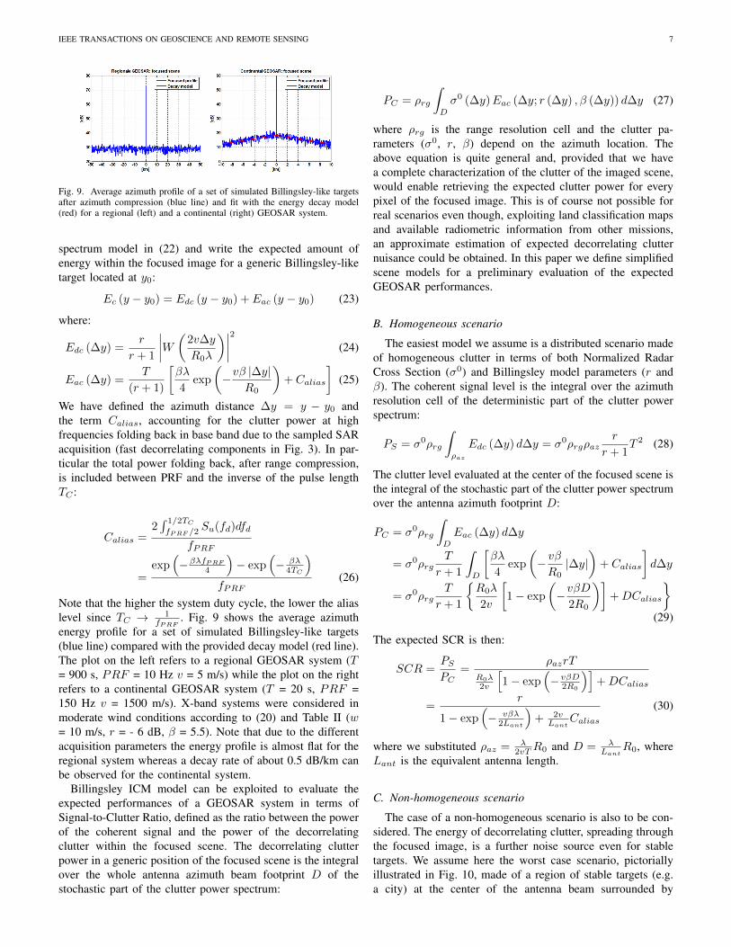
Fig. 9. Average azimuth profile of a set of simulated Billingsley-like targetsafter azimuth compression (blue line) and fit with the energy decay model(red) for a regional (left) and a continental (right) GEOSAR system.

spectrum model in (22) and write the expected amount ofenergy within the focused image for a generic Billingsley-liketarget located at y0:

Ec (y − y0) = Edc (y − y0) + Eac (y − y0) (23)

where:

Edc (∆y) =r

r + 1

∣∣∣∣W (2v∆y

R0λ

)∣∣∣∣2 (24)

Eac (∆y) =T

(r + 1)

[βλ

4exp

(−vβ |∆y|

R0

)+ Calias

](25)

We have defined the azimuth distance ∆y = y − y0 andthe term Calias, accounting for the clutter power at highfrequencies folding back in base band due to the sampled SARacquisition (fast decorrelating components in Fig. 3). In par-ticular the total power folding back, after range compression,is included between PRF and the inverse of the pulse lengthTC :

Calias =2∫ 1/2TC

fPRF /2Su(fd)dfd

fPRF

=exp

(−βλfPRF

4

)− exp

(− βλ

4TC

)fPRF

(26)

Note that the higher the system duty cycle, the lower the aliaslevel since TC → 1

fPRF. Fig. 9 shows the average azimuth

energy profile for a set of simulated Billingsley-like targets(blue line) compared with the provided decay model (red line).The plot on the left refers to a regional GEOSAR system (T= 900 s, PRF = 10 Hz v = 5 m/s) while the plot on the rightrefers to a continental GEOSAR system (T = 20 s, PRF =150 Hz v = 1500 m/s). X-band systems were considered inmoderate wind conditions according to (20) and Table II (w= 10 m/s, r = - 6 dB, β = 5.5). Note that due to the differentacquisition parameters the energy profile is almost flat for theregional system whereas a decay rate of about 0.5 dB/km canbe observed for the continental system.

Billingsley ICM model can be exploited to evaluate theexpected performances of a GEOSAR system in terms ofSignal-to-Clutter Ratio, defined as the ratio between the powerof the coherent signal and the power of the decorrelatingclutter within the focused scene. The decorrelating clutterpower in a generic position of the focused scene is the integralover the whole antenna azimuth beam footprint D of thestochastic part of the clutter power spectrum:

PC = ρrg

∫D

σ0 (∆y)Eac (∆y; r (∆y) , β (∆y)) d∆y (27)

where ρrg is the range resolution cell and the clutter pa-rameters (σ0, r, β) depend on the azimuth location. Theabove equation is quite general and, provided that we havea complete characterization of the clutter of the imaged scene,would enable retrieving the expected clutter power for everypixel of the focused image. This is of course not possible forreal scenarios even though, exploiting land classification mapsand available radiometric information from other missions,an approximate estimation of expected decorrelating clutternuisance could be obtained. In this paper we define simplifiedscene models for a preliminary evaluation of the expectedGEOSAR performances.

B. Homogeneous scenario

The easiest model we assume is a distributed scenario madeof homogeneous clutter in terms of both Normalized RadarCross Section (σ0) and Billingsley model parameters (r andβ). The coherent signal level is the integral over the azimuthresolution cell of the deterministic part of the clutter powerspectrum:

PS = σ0ρrg

∫ρaz

Edc (∆y) d∆y = σ0ρrgρazr

r + 1T 2 (28)

The clutter level evaluated at the center of the focused scene isthe integral of the stochastic part of the clutter power spectrumover the antenna azimuth footprint D:

PC = σ0ρrg

∫D

Eac (∆y) d∆y

= σ0ρrgT

r + 1

∫D

[βλ

4exp

(− vβR0|∆y|

)+ Calias

]d∆y

= σ0ρrgT

r + 1

{R0λ

2v

[1− exp

(−vβD

2R0

)]+DCalias

}(29)

The expected SCR is then:

SCR =PSPC

=ρazrT

R0λ2v

[1− exp

(−vβD2R0

)]+DCalias

=r

1− exp(− vβλ

2Lant

)+ 2v

LantCalias

(30)

where we substituted ρaz = λ2vTR0 and D = λ

LantR0, where

Lant is the equivalent antenna length.

C. Non-homogeneous scenario

The case of a non-homogeneous scenario is also to be con-sidered. The energy of decorrelating clutter, spreading throughthe focused image, is a further noise source even for stabletargets. We assume here the worst case scenario, pictoriallyillustrated in Fig. 10, made of a region of stable targets (e.g.a city) at the center of the antenna beam surrounded by

IEEE TRANSACTIONS ON GEOSCIENCE AND REMOTE SENSING 8

Fig. 10. Non homogeneous clutter scenario for SCR evaluation.

decorrelating clutter (e.g. a forest). The power of the coherentdistributed targets is:

PS = ρrgρazσ0t T

2 (31)

where σ0t is the NRCS of the coherent target. The clutter power

level at the center of the stable region whose extent is a fractionα (0 ≥ α ≥ 1) of the antenna beam width D is:

PC = 2σ0cρrg

∫ D

αD

Eac (∆y) d∆y (32)

where σ0c is the NRCS of the decorrelating clutter. After some

algebra the inverse of the SCR can be written as:

SCR−1 =PCPS

=σ0c

σ0t (r + 1)

2v(1− α)

LantCalias (33)

+σ0c

σ0t (r + 1)

[exp

(− vβαλ

2Lant

)− exp

(− vβλ

2Lant

)]By approximating the exponential terms with the Taylor ex-pansion we can rewrite (33) in a compact way:

SCR−1 =σ0c

σ0t

(1− α)(βλ4 + Calias

)r + 1

2v

Lant(34)

Three terms can be noticed: the first represents the contrast be-tween the reflectivity of clutter and targets, the second dependson the nature of the clutter and the third is system dependent.The previous expression allows to understand which is themost critical nuisance for a GEOSAR system between thermalnoise and clutter. In particular in case the SCR (calculated forσ0t equal the system Noise Equivalent Sigma Zero) is lower

than 1 the system is clutter limited.

V. GEOSAR CASE STUDIES

The SCR models from Section IV allows to derive theexpected performances for a GEOSAR system. In this sectionwe provide a preliminary performance assessment for themain GEOSAR concepts. The calculations are based on theBillingsley ICM model for both the systems even though, asshown in Section III-B, there is little evidence that the modelcan be exploited as it is, especially for a TLCOMP systemwith very long integration times. Nevertheless for a completestatistical characterization of the clutter decorrelation over longobservation times the processing of large amounts of data

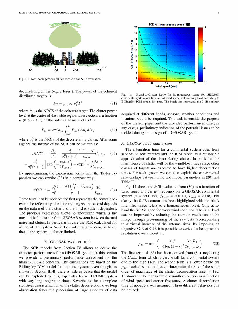
Fig. 11. Signal-to-Clutter Ratio for homogeneous scene for GEOSARcontinental system as a function of wind speed and working band according toBillingsley ICM model for trees. The black line represents the 0 dB contour.

acquired at different bands, seasons, weather conditions andlocations would be required. This task is outside the purposeof the present paper and the provided performances offer, inany case, a preliminary indication of the potential issues to betackled during the design of a GEOSAR system.

A. GEOSAR continental system

The integration time for a continental system goes fromseconds to few minutes and the ICM model is a reasonableapproximation of the decorrelating clutter. In particular themain source of clutter will be the windblown trees since otherclasses of targets are expected to have higher decorrelationtimes. For such system we can also exploit the experimentalrelationships between wind and model parameters in (20) andTable II.

Fig. 11 shows the SCR evaluated from (30) as a function ofwind speed and carrier frequency for a GEOSAR continentalsystem (v = 2600 m/s, fPRF = 200 Hz, Lant = 20 m). Forclarity the 0 dB contour has been highlighted with the blackline. The image refers to a homogeneous forest. Only at L-band the SCR is good for every wind condition. The SCR levelcan be improved by reducing the azimuth resolution of theimage through pre-summing of the raw data (correspondingto a virtual increase of the antenna size). By imposing anobjective SCR of 0 dB it is possible to derive the best possibleresolution over a forest as:

ρaz = min

(− λvβ

4 log (1− r),λτ0R0

2vground

)(35)

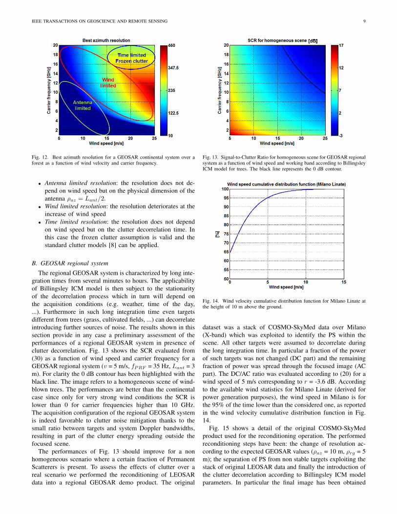
The first term of (35) has been derived from (30), neglectingthe Calias term which is very small for a continental systemdue to the high PRF. The second term is a lower bound forρaz reached when the system integration time is of the sameorder of magnitude of the clutter decorrelation time τ0. Fig.12 shows the best achievable azimuth resolution as a functionof wind speed and carrier frequency. A clutter decorrelationtime of about 3 s was assumed. Three different behaviors canbe noticed:

IEEE TRANSACTIONS ON GEOSCIENCE AND REMOTE SENSING 9

Fig. 12. Best azimuth resolution for a GEOSAR continental system over aforest as a function of wind velocity and carrier frequency.

• Antenna limited resolution: the resolution does not de-pend on wind speed but on the physical dimension of theantenna ρaz = Lant/2.

• Wind limited resolution: the resolution deteriorates at theincrease of wind speed

• Time limited resolution: the resolution does not dependon wind speed but on the clutter decorrelation time. Inthis case the frozen clutter assumption is valid and thestandard clutter models [8] can be applied.

B. GEOSAR regional system

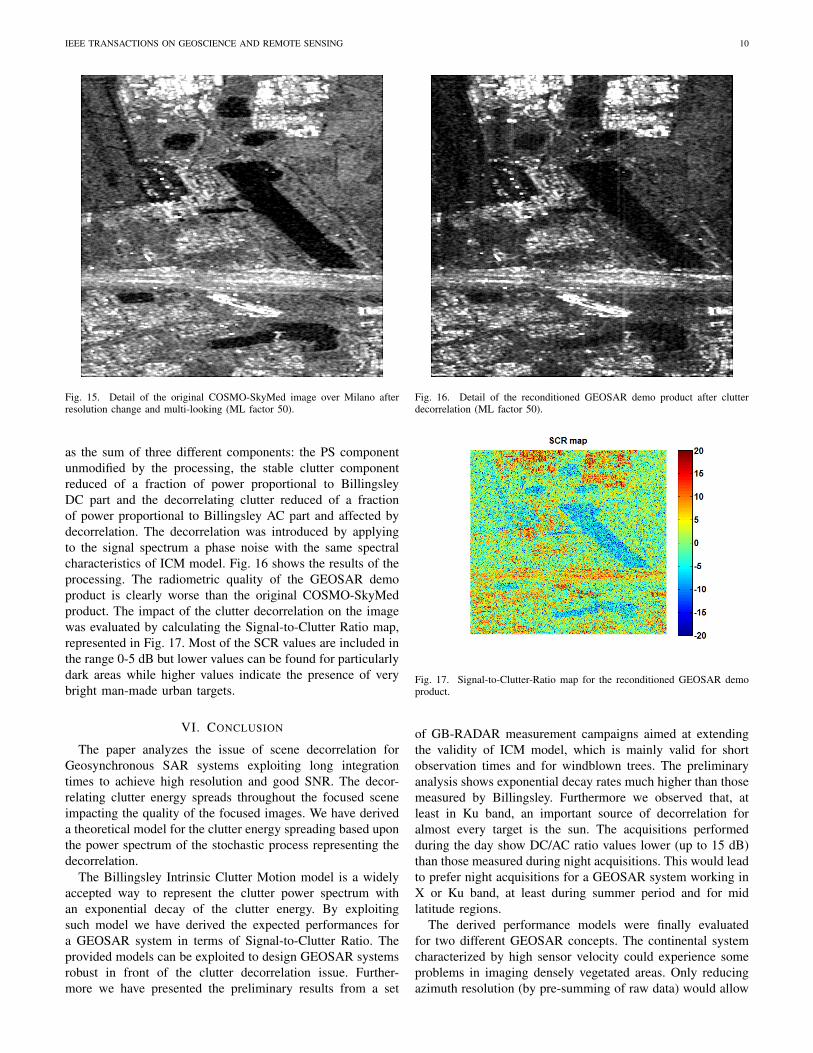
The regional GEOSAR system is characterized by long inte-gration times from several minutes to hours. The applicabilityof Billingsley ICM model is then subject to the stationarityof the decorrelation process which in turn will depend onthe acquisition conditions (e.g. weather, time of the day,...). Furthermore in such long integration time even targetsdifferent from trees (grass, cultivated fields, ...) can decorrelateintroducing further sources of noise. The results shown in thissection provide in any case a preliminary assessment of theperformances of a regional GEOSAR system in presence ofclutter decorrelation. Fig. 13 shows the SCR evaluated from(30) as a function of wind speed and carrier frequency for aGEOSAR regional system (v = 5 m/s, fPRF = 35 Hz, Lant = 3m). For clarity the 0 dB contour has been highlighted with theblack line. The image refers to a homogeneous scene of wind-blown trees. The performances are better than the continentalcase since only for very strong wind conditions the SCR islower than 0 for carrier frequencies higher than 10 GHz.The acquisition configuration of the regional GEOSAR systemis indeed favorable to clutter noise mitigation thanks to thesmall ratio between targets and system Doppler bandwidths,resulting in part of the clutter energy spreading outside thefocused scene.

The performances of Fig. 13 should improve for a nonhomogeneous scenario where a certain fraction of PermanentScatterers is present. To assess the effects of clutter over areal scenario we performed the reconditioning of LEOSARdata into a regional GEOSAR demo product. The original

Fig. 13. Signal-to-Clutter Ratio for homogeneous scene for GEOSAR regionalsystem as a function of wind speed and working band according to BillingsleyICM model for trees. The black line represents the 0 dB contour.

Fig. 14. Wind velocity cumulative distribution function for Milano Linate atthe height of 10 m above the ground.

dataset was a stack of COSMO-SkyMed data over Milano(X-band) which was exploited to identify the PS within thescene. All other targets were assumed to decorrelate duringthe long integration time. In particular a fraction of the powerof such targets was not changed (DC part) and the remainingfraction of power was spread through the focused image (ACpart). The DC/AC ratio was evaluated according to (20) for awind speed of 5 m/s corresponding to r = -3.6 dB. Accordingto the available wind statistics for Milano Linate (derived forpower generation purposes), the wind speed in Milano is forthe 95% of the time lower than the considered one, as reportedin the wind velocity cumulative distribution function in Fig.14.

Fig. 15 shows a detail of the original COSMO-SkyMedproduct used for the reconditioning operation. The performedreconditioning steps have been: the change of resolution ac-cording to the expected GEOSAR values (ρaz = 10 m, ρrg = 5m); the separation of PS from non stable targets exploiting thestack of original LEOSAR data and finally the introduction ofthe clutter decorrelation according to Billingsley ICM modelparameters. In particular the final image has been obtained

IEEE TRANSACTIONS ON GEOSCIENCE AND REMOTE SENSING 10

Fig. 15. Detail of the original COSMO-SkyMed image over Milano afterresolution change and multi-looking (ML factor 50).

as the sum of three different components: the PS componentunmodified by the processing, the stable clutter componentreduced of a fraction of power proportional to BillingsleyDC part and the decorrelating clutter reduced of a fractionof power proportional to Billingsley AC part and affected bydecorrelation. The decorrelation was introduced by applyingto the signal spectrum a phase noise with the same spectralcharacteristics of ICM model. Fig. 16 shows the results of theprocessing. The radiometric quality of the GEOSAR demoproduct is clearly worse than the original COSMO-SkyMedproduct. The impact of the clutter decorrelation on the imagewas evaluated by calculating the Signal-to-Clutter Ratio map,represented in Fig. 17. Most of the SCR values are included inthe range 0-5 dB but lower values can be found for particularlydark areas while higher values indicate the presence of verybright man-made urban targets.

VI. CONCLUSION

The paper analyzes the issue of scene decorrelation forGeosynchronous SAR systems exploiting long integrationtimes to achieve high resolution and good SNR. The decor-relating clutter energy spreads throughout the focused sceneimpacting the quality of the focused images. We have deriveda theoretical model for the clutter energy spreading based uponthe power spectrum of the stochastic process representing thedecorrelation.

The Billingsley Intrinsic Clutter Motion model is a widelyaccepted way to represent the clutter power spectrum withan exponential decay of the clutter energy. By exploitingsuch model we have derived the expected performances fora GEOSAR system in terms of Signal-to-Clutter Ratio. Theprovided models can be exploited to design GEOSAR systemsrobust in front of the clutter decorrelation issue. Further-more we have presented the preliminary results from a set

Fig. 16. Detail of the reconditioned GEOSAR demo product after clutterdecorrelation (ML factor 50).

Fig. 17. Signal-to-Clutter-Ratio map for the reconditioned GEOSAR demoproduct.

of GB-RADAR measurement campaigns aimed at extendingthe validity of ICM model, which is mainly valid for shortobservation times and for windblown trees. The preliminaryanalysis shows exponential decay rates much higher than thosemeasured by Billingsley. Furthermore we observed that, atleast in Ku band, an important source of decorrelation foralmost every target is the sun. The acquisitions performedduring the day show DC/AC ratio values lower (up to 15 dB)than those measured during night acquisitions. This would leadto prefer night acquisitions for a GEOSAR system working inX or Ku band, at least during summer period and for midlatitude regions.

The derived performance models were finally evaluatedfor two different GEOSAR concepts. The continental systemcharacterized by high sensor velocity could experience someproblems in imaging densely vegetated areas. Only reducingazimuth resolution (by pre-summing of raw data) would allow

IEEE TRANSACTIONS ON GEOSCIENCE AND REMOTE SENSING 11

to obtain good quality images. On the contrary the regionalGEOSAR system is more robust to clutter decorrelation thanksto the reduced sensor velocity, resulting in a small scenebandwidth with respect to the system PRF. In any case furtheranalysis on the long term clutter statistics are required for theTLCOMP GEOSAR concept in order to properly account forthe long integration time required by this system.

APPENDIX ATARGETS DECORRELATION MODELS COMPARISON

The coherence between two SAR data x (t) separated by atime interval ∆ is defined as:

γ =E [x (t)x∗(t+ ∆)]√E[|x (t)|2 |x∗(t+ ∆)|

]=E [x (t)x∗(t+ ∆)]

Px=rx(∆)

rx(0)

This expression can be related to the ICM model by evaluatingthe autocorrelation of the clutter power spectral density (18):

rx (t) =1

r + 1

1

1 +(

4πtλβ

)2 +r

r + 1

We can now express the coherence as a function of the theparameters of the ICM model:

γ (∆) =1

r + 1

1

1 +(

4π∆λβ

)2 + r

where, as expected, the coherence is unitary for ∆ = 0 whileγ (∆→ inf) = r

r+1 . The DC/AC parameter defines the longterm coherence, whereas the β parameter describes the shortterm behavior. The long term coherence will be affected byacquisition conditions changes (e.g. wind or day/night).

The DC/AC long term variations can be described exploitingthe models usually assumed for SAR acquisitions. The firstmodel, valid for long observation times, is [26]:

γ(∆t) = exp

(−∆t

τ2

)τ =

λ

4π

√2

σd

derived assuming Brownian motion, that is the displacementsrandomly change with stationary Gaussian increments dis-tributed as N(0, σd). A second model, similar to the firstbut assuming stationary Brownian motion in increments ofvelocity (acceleration) is [27]:

γ(∆t) = exp

(−(

∆t

τ

)2)

τ =λ

4π

√2

σv

where σv is the standard deviation of the velocity increments.Please note that the models have been empirically derived

exploiting spaceborne stacks of interferometric images, withrevisit time of days, whereas in GEOSAR we are interestedin decorrelation times of hours. For this reason, the availableGB-RADAR campaigns should be further exploited to derivea model linking the short term decorrelation described byBillingsley with the long term models derived from spaceborneSAR.

ACKNOWLEDGMENTS

Part of the activities described in the paper was carriedout within the framework of the ESA-ESTEC funded project:Study on Utilization of Future Telecom Satellites for EarthObservation. The authors wish to thank Tazio Strozzi andCharles Werner from GAMMA for performing the radaracquisitions presented in this paper. We also thank MicheleBelotti and Davide Giudici from ARESYS for helping in theprocessing of the GB-RADAR data and in the generation ofthe GEOSAR demo products.

REFERENCES

[1] K. Tomiyasu, “Synthetic aperture radar in geosynchronous orbit,” inAntennas and Propagation Society International Symposium, 1978,vol. 16, 1978, pp. 42–45.

[2] K. Tomiyasu and J. L. Pacelli, “Synthetic aperture radar imaging from aninclined geosynchronous orbit,” Geoscience and Remote Sensing, IEEETransactions on, vol. GE-21, no. 3, pp. 324–329, 1983.

[3] W. N. Edelstein, S. N. Madsen, A. Moussessian, and C. Chen, “Conceptsand technologies for synthetic aperture radar from meo and geosyn-chronous orbits,” Proceedings of SPIE, vol. 5659, 2005.

[4] D. Bruno and S. Hobbs, “Radar imaging from geosynchronous orbit:Temporal decorrelation aspects,” Geoscience and Remote Sensing, IEEETransactions on, vol. 48, no. 7, pp. 2924–2929, 2010.

[5] J. Ruiz Rodon, A. Broquetas, A. Monti Guarnieri, and F. Rocca,“Geosynchronous sar focusing with atmospheric phase screen retrievaland compensation,” Geoscience and Remote Sensing, IEEE Transactionson, vol. 51, no. 8, pp. 4397–4404, 2013.

[6] C. Hu, T. Long, T. Zeng, F. Liu, and Z. Liu, “The accurate focusingand resolution analysis method in geosynchronous sar,” Geoscience andRemote Sensing, IEEE Transactions on, vol. 49, no. 10, pp. 3548–3563,Oct 2011.

[7] Y. Tian, C. Hu, X. Dong, T. Zeng, T. Long, K. Lin, and X. Zhang,“Theoretical analysis and verification of time variation of backgroundionosphere on geosynchronous sar imaging,” Geoscience and RemoteSensing Letters, IEEE, vol. 12, no. 4, pp. 721–725, April 2015.

[8] F. T. Ulaby and M. C. Dobson, Handbook of Radar Scattering Statisticsfor Terrain. Artech House, Inc., Dedham, Massachusetts, 1989.

[9] R. M. M. Walter G. Carrara and R. S. Goodman, Spotlight SyntheticAperture Radar: Signal Processing Algorithms. Artech House RemoteSensing Library, 1995.

[10] M. Wicks, M. Rangaswamy, R. Adve, and T. Hale, “Space-time adaptiveprocessing: a knowledge-based perspective for airborne radar,” SignalProcessing Magazine, IEEE, vol. 23, no. 1, pp. 51–65, Jan 2006.

[11] D. Pastina and F. Turin, “Exploitation of the cosmo-skymed sar systemfor gmti applications,” Selected Topics in Applied Earth Observationsand Remote Sensing, IEEE Journal of, vol. 8, no. 3, pp. 966–979, March2015.

[12] J. Billingsley, Low-angle Radar Land Clutter: Measurementsand Empirical Models, ser. Radar, Sonar, Navigation andAvionics Bks. William Andrew Pub., 2002. [Online]. Available:http://books.google.it/books?id=FEkn0-h7sz0C

[13] A. Recchia, A. Monti Guarnieri, A. Broquetas Ibars, and J. Ruiz Rodon,“Impact of clutter decorrelation on geosynchronous sar,” in EUSAR2014; 10th European Conference on Synthetic Aperture Radar; Pro-ceedings of, June 2014, pp. 1–4.

IEEE TRANSACTIONS ON GEOSCIENCE AND REMOTE SENSING 12

[14] J. Ruiz-Rodon, A. Broquetas, E. Makul, A. Monti-Guarnieri, andA. Recchia, “Internal clutter motion impact on the long integrationgeosar acquisition,” in Geoscience and Remote Sensing Symposium(IGARSS), 2014 IEEE International, July 2014, pp. 2343–2346.

[15] C. Prati, F. Rocca, D. Giancola, and A. Guarnieri, “Passive geosyn-chronous sar system reusing backscattered digital audio broadcast-ing signals,” Geoscience and Remote Sensing, IEEE Transactions on,vol. 36, no. 6, pp. 1973–1976, 1998.

[16] S. Madsen, W. Edelstein, L. DiDomenico, and J. LaBrecque, “Ageosynchronous synthetic aperture radar; for tectonic mapping, disastermanagement and measurements of vegetation and soil moisture,” inGeoscience and Remote Sensing Symposium, 2001. IGARSS ’01. IEEE2001 International, vol. 1, 2001, pp. 447–449 vol.1.

[17] A. Guarnieri, S. Tebaldini, F. Rocca, and A. Broquetas, “Gemini:Geosynchronous sar for earth monitoring by interferometry and imag-ing,” in Geoscience and Remote Sensing Symposium (IGARSS), 2012IEEE International, 2012, pp. 210–213.

[18] L. M. H. Ulander, H. Hellsten, and G. Stenstrom, “Synthetic-apertureradar processing using fast factorized back-projection,” Aerospace andElectronic Systems, IEEE Transactions on, vol. 39, no. 3, pp. 760–776,2003.

[19] A. Recchia, A. Monti Guarnieri, A. Broquetas, and J. Ruiz-Rodon,“Assesment of atmospheric phase screen impact on geosynchronous sar,”in Geoscience and Remote Sensing Symposium (IGARSS), 2014 IEEEInternational, July 2014, pp. 2253–2256.

[20] P. Lombardo and J. B. Billingsley, “A new model for the dopplerspectrum of windblown radar ground clutter,” in Radar Conference,1999. The Record of the 1999 IEEE, 1999, pp. 142–147.

[21] T. Strozzi, A. Wiesmann, and U. Wegmuller, “Gamma’s portable radarinterferometer,” in Symposium on Deformation Measurement and Anal-ysis, Lisbon, 2008.

[22] P. Lombardo, M. Greco, F. Gini, A. Farina, and J. Billingsley, “Impactof clutter spectra on radar performance prediction,” Aerospace andElectronic Systems, IEEE Transactions on, vol. 37, no. 3, pp. 1022–1038, July 2001.

[23] P. Guccione, A. Monti-Guarnieri, and S. Tebaldini, “Stable target detec-tion and coherence estimation in interferometric sar stacks,” Geoscienceand Remote Sensing, IEEE Transactions on, vol. 50, no. 8, pp. 3171–3178, Aug 2012.

[24] L. Iannini and A. Guarnieri, “Atmospheric phase screen in ground-basedradar: Statistics and compensation,” Geoscience and Remote SensingLetters, IEEE, vol. 8, no. 3, pp. 537–541, 2011.

[25] F. De Zan, M. Zonno, P. Lpez-Dekker, and A. Parizzi, “Phase inconsis-tencies and water effects in sar interferometric stacks,” in Proceedingsof Fringe 2015 Workshop, 2015.

[26] F. Rocca, “Modeling interferogram stacks,” Geoscience and RemoteSensing, IEEE Transactions on, vol. 45, no. 10, pp. 3289–3299, Oct2007.

[27] H. Zebker and J. Villasenor, “Decorrelation in interferometric radarechoes,” Geoscience and Remote Sensing, IEEE Transactions on, vol. 30,no. 5, pp. 950–959, Sep 1992.

Andrea Recchia was born in Bergamo, Italy, onJuly 7, 1983. He received the master degree (cumlaude)in Telecommunication Engineering from Po-litecnico di Milano in 2008.

Since 2008 he joined Aresys, a PoliMI spin-off,specialized in radar and geophysics remote sensingsolutions. He is currently part of the SAR R&D teamwith particular interest in SAR data processing, SARdata quality assessment ad future missions designand evaluation.

In 2009 he joined the Synthetic Aperture Radarstudy team at Dipartimento di Elettronica, Informazione e Bioingegneria,Politecnico di Milano. In 2012 he started his PhD (terminated on 2015) aimedat assessing the feasibility of a novel geosynchronous SAR system in presenceof scene and APS decorrelation.

Andrea Monti Guarnieri , M.Sc. cum laude (1988)in electronic engineering, IEEE-member, assistantprofessor and full professor habilitation within Di-partimento di Elettronica, Informazione e Bioingeg-neria. He has been teaching several courses ondigital and statistical signal and image processing,telecommunications and Radar.

Almost forty years of professional activities inSAR systems design and processing, led him in 2003to found Aresys, a PoliMI spin-off, specialized inradar and geophysics remote sensing solutions, then

he served as president up to 2015.His current interests focus on processing and calibration of ground, airborne

and spaceborne SAR, multi-baseline interferometric and MIMO configurationsand geosynchronous SAR.

Prof. Monti Guarnieri co-authored over 200 scientific publications, of which45 international peer reviewed publications, (H-Index 23, 2600 citations);he was awarded three Best Paper in international symposia (IGARSS ’89,EUSAR 2004, EUSAR 2012) and he is co-author of four patents. He isreviewer of journals in remote sensing, signal processing, image processing,geophysics, geodynamics and antennas and propagations, and he has beenin many technical boards of SAR and RADAR conferences. In 2014 he wasappointed by the board of directors member of Technical-scientific Committeeof Italian Space Agency (ASI).

Antoni Broquetas was born in Barcelona, Spain, in1959. He received the Ingeniero degree in Telecom-munication Engineering from the Universitat Politc-nica de Catalunya (UPC) in 1985, and the DoctorIngeniero degree in 1989 in Telecommunications En-gineering for his work on Microwave Tomographyin the UPC.

In 1986 he was a Research Assistant in thePortsmouth Polytechnic (U.K.) involved in propa-gation studies. In 1987 he joined the Department ofSignal Theory and Communications of the School

of Telecommunication Engineering of the UPC in Barcelona.In 1991 started the Remote Sensing research activities at UPC working on

the interferometric applications of Space-borne Synthetic Aperture Radars.From 1998 to 2002 he was Subdirector of Research at the Institute ofGeomatics in Barcelona. From 1999 he is Full Professor in the UPC involvedin research on Radar Imaging and Remote Sensing. From 2003 to 2006 hewas Director of the Signal Theory and Communications Department at UPC.He has published more than 170 papers on Microwave Tomography, Radar,ISAR and SAR systems, SAR processing and Interferometry.

Antonio Leanza received the M.Sc. degree inTelecommunication Engineering from Politecnico diMilano in 2013.

He worked for the remote sensing companyAresys from 2013 to 2014. He is currently a PhDstudent in Information Technology in Politecnico diMilano. His activities focus on Synthetic ApertureRadar and particularly on the analysis of novelGeosynchronous SAR systems for terrain and atmo-sphere observation.