IEEE TRANSACTIONS ON MEDICAL IMAGING, VOL. 28, …pages.ucsd.edu/~ztu/publication/tmi_shi_sulci.pdf · Yonggang Shi, Zhuowen Tu, Allan L. Reiss, Rebecca A. Dutton, Agatha D. Lee,

IEEE TRANSACTIONS ON MEDICAL IMAGING, VOL. 28, NO. 3, MARCH 2009 361

Joint Sulcal Detection on Cortical SurfacesWith Graphical Models and Boosted Priors

Yonggang Shi, Zhuowen Tu, Allan L. Reiss, Rebecca A. Dutton, Agatha D. Lee, Albert M. Galaburda,Ivo Dinov, Paul M. Thompson, and Arthur W. Toga*

Abstract—In this paper, we propose an automated approach forthe joint detection of major sulci on cortical surfaces. By repre-senting sulci as nodes in a graphical model, we incorporate Mar-kovian relations between sulci and formulate their detection as amaximum a posteriori (MAP) estimation problem over the jointspace of major sulci. To make the inference tractable, a samplespace with a finite number of candidate curves is automaticallygenerated at each node based on the Hamilton–Jacobi skeleton ofsulcal regions. Using the AdaBoost algorithm, we learn both in-dividual and pairwise shape priors of sulcal curves from trainingdata, which are then used to define potential functions in the graph-ical model based on the connection between AdaBoost and logisticregression. Finally belief propagation is used to perform the MAPinference and select the joint detection results from the samplespaces of candidate curves. In our experiments, we quantitativelyvalidate our algorithm with manually traced curves and demon-strate the automatically detected curves can capture the main bodyof sulci very accurately. A comparison with independently detectedresults is also conducted to illustrate the advantage of the joint de-tection approach.

Index Terms—AdaBoost, boosted prior, cortex, graphical model,major sulci, shape prior.

I. INTRODUCTION

O NE of the most intriguing and difficult problems in brainimaging is identifying and registering the convolution

patterns of the cortex. It is generally agreed that a set of majorsulci are relatively stable [1] and they have been used as land-mark curves for registration and locating structural and func-tional areas on cortices [2], [3]. On the other hand, the auto-mated detection of these sulci is still a challenging problemdue to the complexity and variability of the convolution pat-terns and the different forms these sulci may have in the foldingpatterns. Thus, manual annotation remains the gold standard in

Manuscript received April 18, 2008; revised July 18, 2008. First publishedAugust 15, 2008; current version published February 25, 2009. This work wassupported by the National Institutes of Health through the NIH Roadmap forMedical Research, Grant U54 RR021813 entitled Center for Computational Bi-ology (CCB). Information on the National Centers for Biomedical Computingcan be obtained from http://nihroadmap.nih.gov/bioinformatics. Asterisk indi-cates corresponding author.

Y. Shi, Z. Tu, R. A. Dutton, A. D. Lee, I. Dinov, and P. M. Thompson are withthe Laboratory of Neuro Imaging, Department of Neurology, UCLA School ofMedicine, Los Angeles, CA 90095 USA.

A. L. Reiss is with the School of Medicine, Stanford University, Stanford,CA 94305 USA.

A. M. Galaburda is with Harvard Medical School, Boston, MA 02215 USA.*A. W. Toga is with the Laboratory of Neuro Imaging, Department of

Neurology, UCLA School of Medicine, Los Angeles, CA 90095 USA (e-mail:[email protected]).

Color versions of one or more of the figures in this paper are available onlineat http://ieeexplore.ieee.org.

Digital Object Identifier 10.1109/TMI.2008.2004402

brain mapping practice. In this paper, we propose a novel ap-proach for the joint detection of major sulci via the solution ofan inference problem on graphical models [4], which we con-struct with boosting techniques [5] to incorporate prior knowl-edge from manual tracing.

Previous work on sulcal detection mostly focused on de-tecting each sulcus separately. Curvature features were firstused to develop semi-automated algorithms [6]–[8] with userspecification of start/end points. Depth features with respect toa shrink wrap surface were also used to study sulcal regionson cortical surfaces [9] or find their line representations [10].Based on the idea of skeletons [11], [12] and digital topology[13]–[15], medial models, or sulcal ribbons, of sulcal regionswere constructed from volume images [16]–[21], but user in-puts are still required to label specific sulcus from these results.

To automate the sulcal detection process, prior models wereintroduced to alleviate the difficulty of the problem. The prin-cipal component analysis (PCA) of point sets [22] was used tomodel the centroids of sulcal basins and help with the labeling[23]. Based on spherical maps of cortical surfaces, a hierarchicalcontour evolution scheme was developed using a PCA model ofmajor sulci [24]. Graphical models were constructed with neuralnetworks in [25] for simple surfaces, which are subsets of majorsulci, computed with the skeletonization algorithm in [16], andthen annealing techniques were used to label them. Based on alearning technique called probabilistic boosting trees [26], anautomated approach was proposed in [27] to detect sulci fromvolume images, but each curve was treated separately.

In this work, we propose a joint detection approach that re-alizes sulcal detection via inference over graphical models ofmajor sulci. We assume that each major sulcus is represented asa continuous curve on the cortical surface following a manualtracing protocol [28]. While this assumption may omit someinterruptions over gyral regions, it is useful in improving theregularity when these curves are used to guide the mapping ofcortical surfaces across population [3]. Based on boosting tech-niques, we not only incorporate the individual shape prior ofeach sulcal curve, but also model joint shape priors betweenneighboring sulci and integrate this information through beliefpropagation. From the practice of manual annotation, the useof pairwise shape priors seems a natural idea. For example, theprecentral sulcus usually needs to cross a gyrus to ensure it fol-lows a route as parallel as possible to the central sulcus. In fact,such local dependencies are utilized fairly commonly to handlecomplicated situations in protocols for manual tracing [28].

As an illustration, we provide an overview of our methodin Fig. 1. In this example, the goal is to detect a set ofeight major sulci on a cortical surface: the central sulcus

0278-0062/$25.00 © 2009 IEEE

Authorized licensed use limited to: Univ of Calif Los Angeles. Downloaded on March 20, 2009 at 23:00 from IEEE Xplore. Restrictions apply.

362 IEEE TRANSACTIONS ON MEDICAL IMAGING, VOL. 28, NO. 3, MARCH 2009

Fig. 1. An overview of our joint sulcal detection approach. The automatically detected sulci are plotted over the cortical surface with the color map on the right.

(CS), precentral sulcus (PreCS), postcentral sulcus (PostCS),superior–frontal sulcus (SF), inferior–frontal sulcus (IF),intraparietal sulcus (IP), sylvian fissure (Sylvian), and the su-perior–temporal sulcus (ST). An undirected graphical modelof eight nodes is used to represent the Markovian relations ofthese sulci. Since the random variable at each node is a sulcalcurve that lives in an infinitely dimensional shape space,it is generally difficult to perform inference directly oversuch spaces. We overcome this challenge by constructing asample space containing a finite number of candidate curves,as plotted over each node in the graph in Fig. 1, greatlyreducing the search range for each variable. To incorporateboth individual and pairwise shape priors, we use boostingtechniques to learn discriminative shape models and use themto define potential functions on the graphical model. Finallythe max-product algorithm of belief propagation is used tofind the MAP estimation from the joint sample spaces of theeight sulci as the sulcal detection results.

Compared with PCA models adopted in previous work [23],[24], the boosting approach we use does not need to imposethe Gaussian assumption on shape models and can automati-cally select and fuse a large set of informative features to modelboth individual and pairwise shape priors. Our prior models arelearned automatically from training data and there is no param-eter to tune for different sulcal curves. Our method also worksdirectly on cortical surfaces and does not need spherical mapsof cortical surfaces [24].

Our work is most related to the sulci labeling algorithm pro-posed in [25], where the nodes of the graph are simple surfacesthat oversample the major sulci and their labeling is realized bymatching with a template graph learned from training data. Inour work, we model each major sulcus as a continuous curve. Inaddition, the learning techniques and inference algorithms usedin our work are different.

The rest of the paper is organized as follows. In Section II,we first present the general framework for joint sulcal detec-tion. After that, we develop the algorithm for generating samplespaces of candidate sulcal curves in Section III. A learning-based approach for constructing potential functions of graph-ical models is proposed in Section IV to model priors of sulcalcurves. Experimental results are presented in Section V on a dataset of 40 surfaces. Finally, we discuss possible future extensionsin Section VI.

II. JOINT DETECTION FRAMEWORK

In this section, we present our general framework for the jointdetection of major sulci on cortical surfaces. By using a graph-ical model to represent Markovian relations of neighboringsulci, we realize automated sulcal detection by performing aMAP estimation over the sample spaces of sulcal lines.

Let denote the cortical surface and be theset of major sulci to be detected on . To represent the Mar-kovian relation among these sulci, we use an undirected graph-ical model , where are theset of nodes, and is the set of edges in the graph. As an ex-ample, a graphical model is shown in Fig. 1 for the eight majorsulci: CS , PreCS , PostCS , SF , IF ,IP , Sylvian , and ST . As the number of majorsulci is typically small, we can construct such graph structureseasily to encode desirable Markovian priors and it only needs tobe done once for the same detection task.

Besides the graph structure, we need to specify the samplespace for the random variable defined at each node and thepotential functions to completely characterize the probabilisticgraphical model. At each node in , the random variable is asulcal line and it can take values in a shape space of curves thatis generally infinitely dimensional and difficult to analyze. Onepossible solution is to use dimension reduction techniques suchas PCA models of curves [22] to generate each sulcal line asa linear combination of several basis functions. But the PCAmodels make the restrictive assumption of Gaussian distribu-tions and there is no guarantee that the generated parametriccurves will follow the sulcal regions. To overcome this problem,we develop a novel algorithm, which will be described in detailin Section III, to automatically generate a set of candidate curvesfor each node by combining geometric features of sulcal regionsand machine learning techniques. These curves are guaranteedto be on the cortical surface and they span a wide variety ofpossible routes for each sulcus of interest. With these candidatecurves as the sample space of each node , we convert thesulcal detection problem to a tractable inference problem overa set of discrete random variables with the goal of selecting thebest from the candidate curves.

Based on the sample spaces of candidate sulcal curves, wedefine two types of potential functions to complete the con-struction of the graphical model: the local evidence function


SHI et al.: JOINT SULCAL DETECTION ON CORTICAL SURFACES WITH GRAPHICAL MODELS AND BOOSTED PRIORS 363

at each node and the compatibility functionfor each edge . Given a can-

didate curve from , the local evidence function gives thelikelihood of this curve being the desirable sulcus to be detected.The compatibility function represents joint shape priors fortwo neighboring sulci and measures how likely anytwo curves from can co-exist as neighbors. To incor-porate such individual and joint shape priors, we propose a dis-criminative approach based on AdaBoost [5] in Section IV tolearn both types of potential functions from manually annotatedtraining data. With the discriminative approach, we can use aflexible and large set of features derived from training data andselectively combine them with boosting techniques to form thepotential functions, so there is no need of specifying parametricforms for either the individual or joint shape prior models ofsulcal lines.

The undirected graphical model defined above is a Markovrandom field, so the joint distribution of all the sulci can befactorized as a product of potential functions

(1)

where is the partition function for normalization. The task offinding the optimal set of curves in the space

is then a MAP estimation problem definedas follows:

(2)

To solve this inference problem over graphical models, we usethe max-product algorithm of belief propagation [4], [29] be-cause it can efficiently compute the optimal solution for tree-structured graphs and also demonstrated very good performanceon graphs with cycles in various applications [30], [31]. Withbelief propagation, each node in the graph receives and sendsout messages at every iteration of the algorithm. For a node ,the message it sends to its neighbor is defined as

(3)

where are neighbors of in the graph. This messagetakes into account not only the local evidence and the com-patibility function , but also the messages the node re-ceived from its neighbors except . As an illustration, we showin Fig. 2 the flow of messages from the node and to ,and then to in the graphical model shown in Fig. 1. After themessage passing procedure converges, we obtain the final beliefat each node of the graph as

(4)

Fig. 2. An example of message passing in the graphical model of Fig. 1.

and also the pairwise belief of each edge as

(5)

Based on the final beliefs, we find an optimal configuration ofmajor sulci with the following procedure [32], [33].

1) Start from a node and pick the optimal sulcus at thisnode as the one that maximizes .

2) For each node visited, if it has a neighbor unvisited,find the optimal solution for by maximizing the pair-wise belief function . Repeatstep 2 until all nodes are visited.

For tree-structured graphs, the above algorithm guaranteesto find the globally optimal solution for the MAP estimationproblem in (2). It is possible that more than one solutionachieves global optimality for MAP estimation over graphs,but in our experience this does not happen in any of our sulcidetection experiments. Nevertheless, we choose to fix thestarting node as the one corresponding to the central sulcus instep 1 of the above procedure to remove the potential ambiguitythat exists theoretically.

III. SAMPLE SPACE GENERATION

Given a cortical surface represented as a genus zero tri-angular mesh, which we assume is a left hemispheric surfacealigned in a standard ICBM space [34] with a nine-parameteraffine registration including independent scaling in -, -, and

- directions to account for brain size differences, there are fourmain steps in our algorithm to generate a sample space for eachnode in the graphical model: 1) extract the skeleton of the sulcalregions; 2) partition the surface into the lateral and medial part;3) compute a set of possible start/end points and route-controlsegments of candidate curves with a learning-based approach;4) generate candidate curves via random walks on a graph builtfrom the start/end points and route-control segments.

A. Sulcal Skeleton Extraction

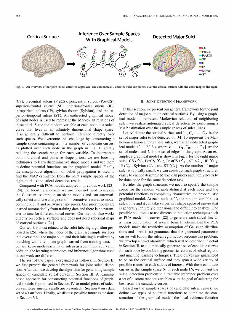
As a first stage toward sample space generation, we use thealgorithm of computing Hamilton–Jacobi skeletons on corticalsurfaces [35] to extract the skeleton of sulcal regions on . Forcompleteness, we briefly describe the main steps of computingthe sulcal skeletons as illustrated in Fig. 3. Using the mean cur-vature of the cortical surface , it is first partitioned into sulcaland gyral regions using graph cuts [36], [37] and the result isshown in Fig. 3(b). After that, the Hamilton–Jacobi skeletonmethod [38] is extended to triangular meshes to compute the



Fig. 3. Main steps in computing the sulcal skeletons of a cortical surface. (a) The cortical surface. (b) The partition of the surface into sulcal and gyral regions.(c) The Hamilton-Jacobi skeleton of the sulcal regions. End points of each branch are marked as green dots.

skeleton of sulcal regions. A pruning process is finally applied toeliminate small branches with length below a specific threshold,which is 10 mm in all our experiments. The sulcal skeletons aredecomposed into a set of branches as shown in Fig. 3(c), wherewe have plotted the main body of the branches in blue and theend points in green. From the results we can see these sulcalskeletons capture the major folding patterns fairly well and pro-vide a compact summary of cortex geometry.

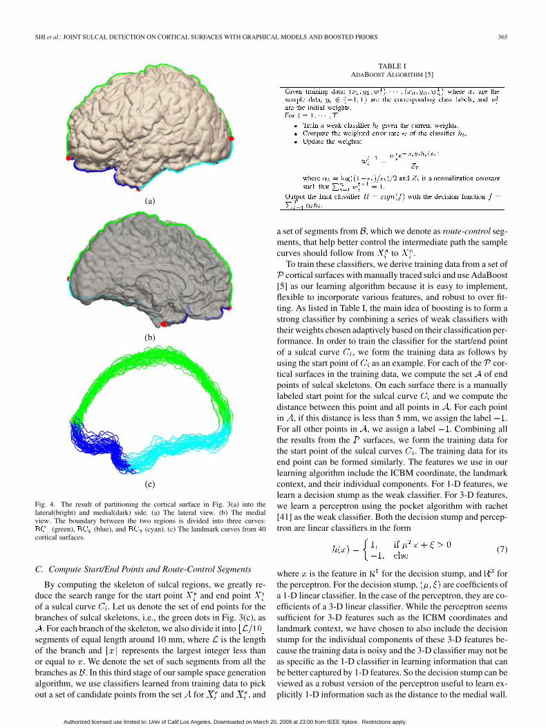
B. Lateral/Medial Side Partition

In the second stage we partition the hemispheric cortical sur-face into lateral and medial parts with a graph-cut algo-rithm. The resulting boundary between the lateral and medialside is then used to compute a set of features with the aim ofproviding intrinsic information about sulcal features in additionto absolute coordinates (in millimeter) in the ICBM space andimproving the robustness to pose variations.

Before we apply the graph-cut algorithm, we first find a set ofseed points for both the lateral and medial side. Since is a lefthemispheric surface in the ICBM space, where the -coordinateincreases from left to right, we find a set of seed points forthe lateral side as vertices visible from the left side, i.e., the“ ” direction, using the -buffer algorithm for visible surfacedetermination in computer graphics. Similarly, the set of seedpoints for the medial side are determined as vertices visiblefrom the right side, i.e., the “- ” direction.

Because there are hidden regions invisible from either the leftor right side, the two sets and do not form a completepartition of the surface. To achieve this goal, we minimize thefollowing energy function to separate into the lateral sideand the medial side :

(6)

where and are vertices on is the total numberof vertices, denote the geodesic distance between twopoint sets on that can be computed numerically with the fastmarching algorithm on triangular meshes [39], and the deltafunction is defined as one when and , a vertex in itsone-ring neighborhood , belong to different regions andzero otherwise. The first two energy terms require and

to be close to their seed points, the third energy term providesregularization for boundary smoothness and the nonnegative pa-rameter controls the weight of regularization. To minimize theenergy, the same graph-cut algorithm used in stage one for parti-tioning into sulcal and gyral regions is applied to find the so-lution. Since this is a binary optimization problem, the graph-cuttechnique ensures the global optimality of the separation result[36], [37].

As an example, we show in Fig. 4 the partition results forthe surface in Fig. 3(a). Choosing a proper regularization pa-rameter ensures there will be no holes in and and theirboundary is a simple curve. In our experience, the parameter

gives very robust performance. With this parameter, ouralgorithm is able to successfully partition all of the 40 corticalsurfaces used our experiments into only two connected compo-nents corresponding to the lateral and medial parts.

Once we have the partition results and , we find threeboundary vertices, shown as red dots in Fig. 4, that have thelargest -coordinate, the smallest -coordinate, and the smallest

-coordinate, respectively, and use them to divide the boundarybetween and into three curves shownas the green, blue, and cyan curve in Fig. 4(a) and (b). We havealso plotted the three curves from all 40 surfaces used in ourexperiments in Fig. 4(c). We can see these curves are clusteredfairly closely in the ICBM space and this helps demonstrate therobustness of our partition algorithm. Using these three curves,we can compute the landmark context feature [40] defined ateach vertex as to provide an intrinsiccharacterization of locations on , whereis the geodesic distance to the curve . While the landmarkcontext feature is not necessarily unique over the surface, it pro-vides very intuitive characterizations of the intrinsic locations ofmajor sulci on the cortical surface using distances to the threecurves. For example, the distance to the curve is usefulin describing the almost parallel path to the medial wall the SFsulcus usually takes. This distance is also useful to describe themedial-to-lateral trend of the CS, PreCS, and PostCS. The dis-tance to the curve is valuable in characterizing the intrinsiclocation of the frontal part of the SF, IF, ST sulcus and the syl-vian fissure. With the distance to the curve , we can quantifyeffectively the almost parallel relation between the ST sulcusand the sylvian fissure. In the next stage, we will use both theICBM coordinate and the landmark context feature to charac-terize relative locations on for the learning algorithms.



Fig. 4. The result of partitioning the cortical surface in Fig. 3(a) into thelateral(bright) and medial(dark) side. (a) The lateral view. (b) The medialview. The boundary between the two regions is divided into three curves:�� (green), �� (blue), and �� (cyan). (c) The landmark curves from 40cortical surfaces.

C. Compute Start/End Points and Route-Control Segments

By computing the skeleton of sulcal regions, we greatly re-duce the search range for the start point and end pointof a sulcal curve . Let us denote the set of end points for thebranches of sulcal skeletons, i.e., the green dots in Fig. 3(c), as

. For each branch of the skeleton, we also divide it intosegments of equal length around 10 mm, where is the lengthof the branch and represents the largest integer less thanor equal to . We denote the set of such segments from all thebranches as . In this third stage of our sample space generationalgorithm, we use classifiers learned from training data to pickout a set of candidate points from the set for and , and

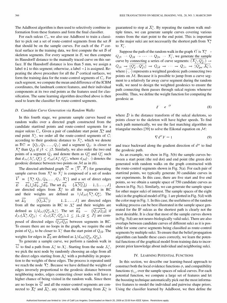
TABLE IADABOOST ALGORITHM [5]

a set of segments from , which we denote as route-control seg-ments, that help better control the intermediate path the samplecurves should follow from to .

To train these classifiers, we derive training data from a set ofcortical surfaces with manually traced sulci and use AdaBoost

[5] as our learning algorithm because it is easy to implement,flexible to incorporate various features, and robust to over fit-ting. As listed in Table I, the main idea of boosting is to form astrong classifier by combining a series of weak classifiers withtheir weights chosen adaptively based on their classification per-formance. In order to train the classifier for the start/end pointof a sulcal curve , we form the training data as follows byusing the start point of as an example. For each of the cor-tical surfaces in the training data, we compute the set of endpoints of sulcal skeletons. On each surface there is a manuallylabeled start point for the sulcal curve and we compute thedistance between this point and all points in . For each pointin , if this distance is less than 5 mm, we assign the label .For all other points in , we assign a label . Combining allthe results from the surfaces, we form the training data forthe start point of the sulcal curves . The training data for itsend point can be formed similarly. The features we use in ourlearning algorithm include the ICBM coordinate, the landmarkcontext, and their individual components. For 1-D features, welearn a decision stump as the weak classifier. For 3-D features,we learn a perceptron using the pocket algorithm with rachet[41] as the weak classifier. Both the decision stump and percep-tron are linear classifiers in the form

(7)

where is the feature in for the decision stump, and forthe perceptron. For the decision stump, are coefficients ofa 1-D linear classifier. In the case of the perceptron, they are co-efficients of a 3-D linear classifier. While the perceptron seemssufficient for 3-D features such as the ICBM coordinates andlandmark context, we have chosen to also include the decisionstump for the individual components of these 3-D features be-cause the training data is noisy and the 3-D classifier may not beas specific as the 1-D classifier in learning information that canbe better captured by 1-D features. So the decision stump can beviewed as a robust version of the perceptron useful to learn ex-plicitly 1-D information such as the distance to the medial wall.



The AdaBoost algorithm is then used to selectively combine in-formation from these features and form the final classifier.

For each sulcus , we also use AdaBoost to train a classi-fier to pick out a set of route-control segments from the setthat should be on the sample curves. For each of the cor-tical surface in the training data, we first compute the set ofskeleton segments. For every segment in , we then computeits Hausdorff distance to the manually traced curve on this sur-face. If the Hausdorff distance is less than 5 mm, we assign alabel to this segment; otherwise, a label is assigned. Re-peating the above procedure for all the cortical surfaces, weform the training data for the route-control segments of . Foreach segment, we compute the mean and difference of the ICBMcoordinates, the landmark context features, and their individualcomponents at its two end points as the features used for clas-sification. The same learning algorithm described above is thenused to learn the classifier for route-control segments.

D. Candidate Curve Generation via Random Walks

In this fourth stage, we generate sample curves based onrandom walks over a directed graph constructed from thecandidate start/end points and route-control segments for amajor sulcus . Given a pair of candidate start point andend point , we order all the route-control segments ofaccording to their geodesic distance to , which we denoteas and a segment is closer to

than if . Similarly, we also order the two endpoints of a segment and denote them as and suchthat , where denotes thegeodesic distance between two points on as in (6).

The directed attributed graph for generatingsample curves from to is composed of a set of nodes

and a set of direct edges

. The setare directed edges from to all the segments in RCand their weights are defined as . The

set are directed edgesfrom all the segments in RC to and their weights are

defined as . The set ifare com-

posed of directed edges between segments in RC.To ensure there are no loops in the graph, we require the endpoint of to be closer to than the start point of . The

weights for edges in are defined as .To generate a sample curve, we perform a random walk in

to find a path from to . Starting from the node ,we pick the next node by randomly choosing an edge from allthe direct edges starting from with a probability in propor-tion to the weights of these edges. The process is repeated untilwe reach the node . Because we have defined the weights ofedges inversely proportional to the geodesic distance betweenneighboring nodes, edges connecting closer nodes will have ahigher chance of being visited in the random walk. Since there

are no loops in and all the router-control segments are con-nected to and , any random walk starting from is

guaranteed to stop at . By repeating the random walk mul-tiple times, we can generate sample curves covering variousroutes from the start point to the end point. This is importantas the major sulci are not necessarily the shortest path fromto .

Suppose the path of the random walk in the graph is, we generate the sample

curve by connecting a series of curve segments:,

where represents a weighted geodesic path connecting twopoints on . Because it is possible to jump from a curve seg-ment to a relatively far away curve segment during the randomwalk, we need to design the weighted geodesics to ensure thepath connecting them passes through sulcal regions wheneverpossible. Thus, we define the weight function for computing thegeodesic as

(8)

where is the distance transform of the sulcal skeletons, sopoints closer to the skeleton will have higher speeds. To findeach path numerically, we use the fast marching algorithm ontriangular meshes [39] to solve the Eikonal equation on :

(9)

and trace backward along the gradient direction of to findthe geodesic path.

As an example, we show in Fig. 5(b) the sample curves be-tween a start point (the red dot) and end point (the green dot)generated with random walks on the graph constructed withthe route-control segments shown in Fig. 5(a). For each pair ofstart/end points, we typically generate 30 candidate curves inour experiments. In this case, there are five start and five endpoints, so we obtain a sample space of 750 candidate curves asshown in Fig. 5(c). Similarly, we can generate the sample spacefor other major sulci of interest. The sample spaces of the eightsulci in the graphical model of Fig. 1 are plotted in Fig. 5(d) withthe color map in Fig. 1. In this case, the usefulness of the randomwalking process can be best illustrated in the sample space gen-erated for the IF sulcus as the shortest path is clearly not themost desirable. It is clear that most of the sample curves shownin Fig. 5(d) are not neuro-biologically valid sulci. There are alsooverlaps between candidate curves of different sulci as it is pos-sible for some curve segments being classified as route-controlsegments by multiple sulci. To ensure that the belief propagationalgorithm can handle these cases correctly, we learn the poten-tial functions of the graphical model from training data to incor-porate prior knowledge about individual and neighboring sulci.

IV. LEARNING POTENTIAL FUNCTIONS

In this section, we describe our learning-based approach toconstruct both the local evidence functions and compatibilityfunctions over the sample spaces of sulcal curves. For eachpotential function, we compute a large set of features and letthe boosting technique automatically pick out the most informa-tive features to model the individual and pairwise shape priors.Using the classifier learned by AdaBoost, we then define the



Fig. 5. The process of sample space generation. (a) The candidate start (red) and end (green) points of the precentral sulcus, and its route-control segments whoseboth ends are marked as yellow dots. (b) The sample curves generated with 30 random walks between a pair of start and end points of the precentral sulcus. (c) Thesample space of precentral sulcus as composed of curves connecting all the start and end points. (d) The sample spaces of all eight major sulci in the graphicalmodel of Fig. 1 are plotted with the same color map in Fig. 1.

potential function based on its connection to logistic regression[42].

For both the local evidence functions and compatibility func-tions, we assume a training data set of cortical surfaces in theICBM space with manually labeled sulcal lines. For each sur-face, we compute the sample space for each node in thegraphical model.

A. Local Evidence Functions

To learn the local evidence function for a sulcus , weform its training data as follows. We assign all the manuallytraced curves on the surfaces the label . For a curve from

of each surface, we assign it the label if more than 50%of the points on the curve have a minimum distance of 10 mmto the corresponding manually traced sulcus.

To characterize these curves, we use the Haar wavelet trans-form to compute a set of multiscale features. More specifically,we uniformly sample each curve into points. TheHaar wavelet transform is then computed for the ICBM coor-dinates, landmark context features, and their individual com-ponents defined at these uniformly sample points. As a result,we have 3-D features from the ICBM coordinates andlandmark context features, and 1-D features from theirindividual components. This large set of features provides amulti-scale description of the location and orientation of thecurves.

Using these features, the AdaBoost algorithm combines a se-ries of weak classifiers to form a final decision function for acurve

(10)

where is the th weak classifier, which is a decision stump for1-D features and perceptron for 3-D features, is the weight forthis classifier, and is the total number of weak classifiers. It isshown in [42] that AdaBoost approximates logistic regressionand the learned decision function can be used to estimate theprobability of a class label, thus we follow [42] and define thelocal evidence function as

(11)

The range of the local evidence function is between (0,1) and itapproaches 1 when is large for a curve , whichsuggests this curve bears strong similarity to manually tracedsulcal lines in the training data. On the other hand, it approacheszero for curves with negative decision function values.

B. Compatibility Functions

For two nodes and in the graphical model , we followa similar process to learn their compatibility function , butwith a different set of features to capture their joint shape priors.Given a cortical surface, we generate the sample spaces and

for these two sulci, and the value measures howcompatible a pair of curves being the twomajor sulci. The training data to learn thus are also com-posed of curve pairs that we form as follows. For the

pairs of manually traced sulci for and on the surfacesin the training data, we assign a label . For each of the sur-face, we compute the sample space and and assign a label

for the set of curve pairs generated by associatingeach curve with a randomly picked curve withthe goal of representing possible cases of incompatible curves.By repeating the above procedure for each edge in the graph-ical model , we can generate different training data for otherneighboring sulci.

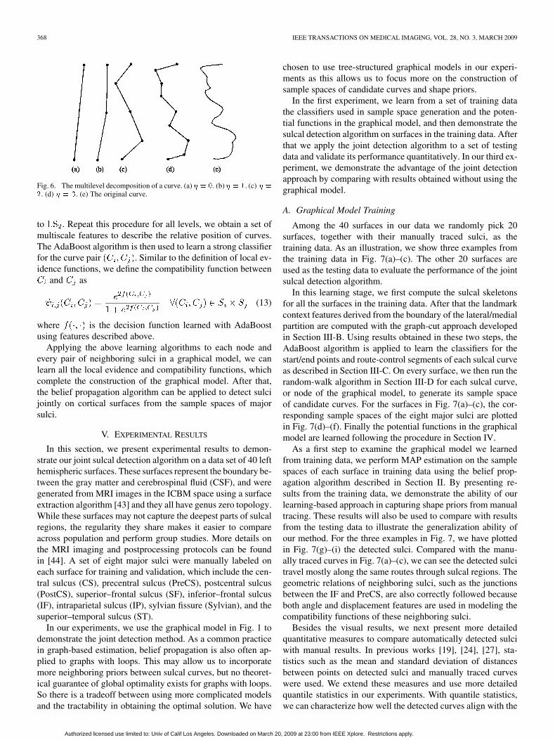
As inputs to the weak classifiers used in AdaBoost, we de-sign a set of multiscale features to model the joint configurationfor each pair of curves . Let denote the maximumnumber of levels we want to compute the features. We resampleeach curve and into equally spaced points. Let

be the points on , we then approximateit with a set of straight line segments at the level

(12)

where denote the line segment connectingthe two points and . As shown in Fig. 6, linesegments at the coarse scale captures the global trend of eachcurve, while the line segments at finer scales provide more localinformation. Similarly, the curve is also decomposed into thesame number of levels and we use the relation between line seg-ments from these two curves to characterize their configurationat each level. More specifically, for each line segment of

and of at a level , we compute the angle betweenthem and the shortest displacement vector from points on



Fig. 6. The multilevel decomposition of a curve. (a) � � �. (b) � � �. (c) � ��. (d) � � �. (e) The original curve.

to . Repeat this procedure for all levels, we obtain a set ofmultiscale features to describe the relative position of curves.The AdaBoost algorithm is then used to learn a strong classifierfor the curve pair . Similar to the definition of local ev-idence functions, we define the compatibility function between

and as

(13)

where is the decision function learned with AdaBoostusing features described above.

Applying the above learning algorithms to each node andevery pair of neighboring sulci in a graphical model, we canlearn all the local evidence and compatibility functions, whichcomplete the construction of the graphical model. After that,the belief propagation algorithm can be applied to detect sulcijointly on cortical surfaces from the sample spaces of majorsulci.

V. EXPERIMENTAL RESULTS

In this section, we present experimental results to demon-strate our joint sulcal detection algorithm on a data set of 40 lefthemispheric surfaces. These surfaces represent the boundary be-tween the gray matter and cerebrospinal fluid (CSF), and weregenerated from MRI images in the ICBM space using a surfaceextraction algorithm [43] and they all have genus zero topology.While these surfaces may not capture the deepest parts of sulcalregions, the regularity they share makes it easier to compareacross population and perform group studies. More details onthe MRI imaging and postprocessing protocols can be foundin [44]. A set of eight major sulci were manually labeled oneach surface for training and validation, which include the cen-tral sulcus (CS), precentral sulcus (PreCS), postcentral sulcus(PostCS), superior–frontal sulcus (SF), inferior–frontal sulcus(IF), intraparietal sulcus (IP), sylvian fissure (Sylvian), and thesuperior–temporal sulcus (ST).

In our experiments, we use the graphical model in Fig. 1 todemonstrate the joint detection method. As a common practicein graph-based estimation, belief propagation is also often ap-plied to graphs with loops. This may allow us to incorporatemore neighboring priors between sulcal curves, but no theoret-ical guarantee of global optimality exists for graphs with loops.So there is a tradeoff between using more complicated modelsand the tractability in obtaining the optimal solution. We have

chosen to use tree-structured graphical models in our experi-ments as this allows us to focus more on the construction ofsample spaces of candidate curves and shape priors.

In the first experiment, we learn from a set of training datathe classifiers used in sample space generation and the poten-tial functions in the graphical model, and then demonstrate thesulcal detection algorithm on surfaces in the training data. Afterthat we apply the joint detection algorithm to a set of testingdata and validate its performance quantitatively. In our third ex-periment, we demonstrate the advantage of the joint detectionapproach by comparing with results obtained without using thegraphical model.

A. Graphical Model Training

Among the 40 surfaces in our data we randomly pick 20surfaces, together with their manually traced sulci, as thetraining data. As an illustration, we show three examples fromthe training data in Fig. 7(a)–(c). The other 20 surfaces areused as the testing data to evaluate the performance of the jointsulcal detection algorithm.

In this learning stage, we first compute the sulcal skeletonsfor all the surfaces in the training data. After that the landmarkcontext features derived from the boundary of the lateral/medialpartition are computed with the graph-cut approach developedin Section III-B. Using results obtained in these two steps, theAdaBoost algorithm is applied to learn the classifiers for thestart/end points and route-control segments of each sulcal curveas described in Section III-C. On every surface, we then run therandom-walk algorithm in Section III-D for each sulcal curve,or node of the graphical model, to generate its sample spaceof candidate curves. For the surfaces in Fig. 7(a)–(c), the cor-responding sample spaces of the eight major sulci are plottedin Fig. 7(d)–(f). Finally the potential functions in the graphicalmodel are learned following the procedure in Section IV.

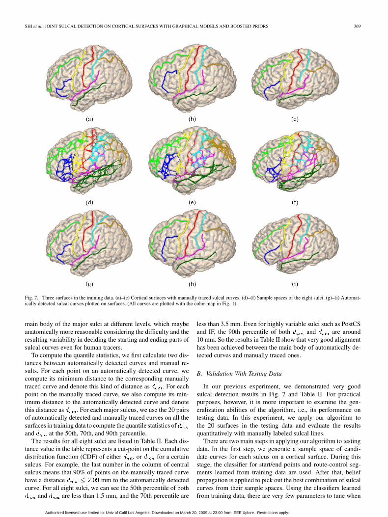
As a first step to examine the graphical model we learnedfrom training data, we perform MAP estimation on the samplespaces of each surface in training data using the belief prop-agation algorithm described in Section II. By presenting re-sults from the training data, we demonstrate the ability of ourlearning-based approach in capturing shape priors from manualtracing. These results will also be used to compare with resultsfrom the testing data to illustrate the generalization ability ofour method. For the three examples in Fig. 7, we have plottedin Fig. 7(g)–(i) the detected sulci. Compared with the manu-ally traced curves in Fig. 7(a)–(c), we can see the detected sulcitravel mostly along the same routes through sulcal regions. Thegeometric relations of neighboring sulci, such as the junctionsbetween the IF and PreCS, are also correctly followed becauseboth angle and displacement features are used in modeling thecompatibility functions of these neighboring sulci.

Besides the visual results, we next present more detailedquantitative measures to compare automatically detected sulciwith manual results. In previous works [19], [24], [27], sta-tistics such as the mean and standard deviation of distancesbetween points on detected sulci and manually traced curveswere used. We extend these measures and use more detailedquantile statistics in our experiments. With quantile statistics,we can characterize how well the detected curves align with the



Fig. 7. Three surfaces in the training data. (a)–(c) Cortical surfaces with manually traced sulcal curves. (d)–(f) Sample spaces of the eight sulci. (g)–(i) Automat-ically detected sulcal curves plotted on surfaces. (All curves are plotted with the color map in Fig. 1).

main body of the major sulci at different levels, which maybeanatomically more reasonable considering the difficulty and theresulting variability in deciding the starting and ending parts ofsulcal curves even for human tracers.

To compute the quantile statistics, we first calculate two dis-tances between automatically detected curves and manual re-sults. For each point on an automatically detected curve, wecompute its minimum distance to the corresponding manuallytraced curve and denote this kind of distance as . For eachpoint on the manually traced curve, we also compute its min-imum distance to the automatically detected curve and denotethis distance as . For each major sulcus, we use the 20 pairsof automatically detected and manually traced curves on all thesurfaces in training data to compute the quantile statistics ofand at the 50th, 70th, and 90th percentile.

The results for all eight sulci are listed in Table II. Each dis-tance value in the table represents a cut-point on the cumulativedistribution function (CDF) of either or for a certainsulcus. For example, the last number in the column of centralsulcus means that 90% of points on the manually traced curvehave a distance mm to the automatically detectedcurve. For all eight sulci, we can see the 50th percentile of both

and are less than 1.5 mm, and the 70th percentile are

less than 3.5 mm. Even for highly variable sulci such as PostCSand IF, the 90th percentile of both and are around10 mm. So the results in Table II show that very good alignmenthas been achieved between the main body of automatically de-tected curves and manually traced ones.

B. Validation With Testing Data

In our previous experiment, we demonstrated very goodsulcal detection results in Fig. 7 and Table II. For practicalpurposes, however, it is more important to examine the gen-eralization abilities of the algorithm, i.e., its performance ontesting data. In this experiment, we apply our algorithm tothe 20 surfaces in the testing data and evaluate the resultsquantitatively with manually labeled sulcal lines.

There are two main steps in applying our algorithm to testingdata. In the first step, we generate a sample space of candi-date curves for each sulcus on a cortical surface. During thisstage, the classifier for start/end points and route-control seg-ments learned from training data are used. After that, beliefpropagation is applied to pick out the best combination of sulcalcurves from their sample spaces. Using the classifiers learnedfrom training data, there are very few parameters to tune when



TABLE IIQUANTILE STATISTICS OF � AND � FROM SULCI DETECTED IN TRAINING DATA. ALL DISTANCES ARE IN MILLIMETERS

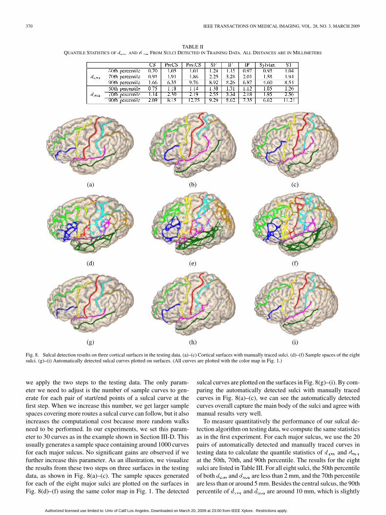
Fig. 8. Sulcal detection results on three cortical surfaces in the testing data. (a)–(c) Cortical surfaces with manually traced sulci. (d)–(f) Sample spaces of the eightsulci. (g)–(i) Automatically detected sulcal curves plotted on surfaces. (All curves are plotted with the color map in Fig. 1.)

we apply the two steps to the testing data. The only param-eter we need to adjust is the number of sample curves to gen-erate for each pair of start/end points of a sulcal curve at thefirst step. When we increase this number, we get larger samplespaces covering more routes a sulcal curve can follow, but it alsoincreases the computational cost because more random walksneed to be performed. In our experiments, we set this param-eter to 30 curves as in the example shown in Section III-D. Thisusually generates a sample space containing around 1000 curvesfor each major sulcus. No significant gains are observed if wefurther increase this parameter. As an illustration, we visualizethe results from these two steps on three surfaces in the testingdata, as shown in Fig. 8(a)–(c). The sample spaces generatedfor each of the eight major sulci are plotted on the surfaces inFig. 8(d)–(f) using the same color map in Fig. 1. The detected

sulcal curves are plotted on the surfaces in Fig. 8(g)–(i). By com-paring the automatically detected sulci with manually tracedcurves in Fig. 8(a)–(c), we can see the automatically detectedcurves overall capture the main body of the sulci and agree withmanual results very well.

To measure quantitatively the performance of our sulcal de-tection algorithm on testing data, we compute the same statisticsas in the first experiment. For each major sulcus, we use the 20pairs of automatically detected and manually traced curves intesting data to calculate the quantile statistics of andat the 50th, 70th, and 90th percentile. The results for the eightsulci are listed in Table III. For all eight sulci, the 50th percentileof both and are less than 2 mm, and the 70th percentileare less than or around 5 mm. Besides the central sulcus, the 90thpercentile of and are around 10 mm, which is slightly



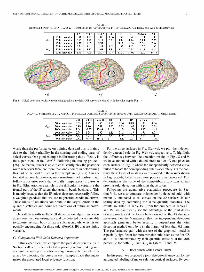
TABLE IIIQUANTILE STATISTICS OF � AND � FROM SULCI DETECTED JOINTLY IN TESTING DATA. ALL DISTANCES ARE IN MILLIMETERS

Fig. 9. Sulcal detection results without using graphical models. (All curves are plotted with the color map in Fig. 1).

TABLE IVQUANTILE STATISTICS OF � AND � FROM SULCI DETECTED SEPARATELY IN TESTING DATA. ALL DISTANCES ARE IN MILLIMETERS

worse than the performance on training data and this is mainlydue to the high variability in the starting and ending parts ofsulcal curves. One good example in illustrating this difficulty isthe superior end of the PostCS. Following the tracing protocol[28], the manual tracer is able to consistently pick the posteriorroute whenever there are more than one choices in determiningthis part of the PostCS such as the example in Fig. 7(a). Our au-tomated approach, however, may sometimes get confused andfollow a posterior route that actually jumps across a gyrus asin Fig. 8(h). Another example is the difficulty in capturing thefrontal part of the IF sulcus that usually bends backward. Thisis mainly because that the IF sulcus does not necessarily followa weighted geodesic that we use to generate candidate curves.These kinds of situations contribute to the largest errors in thequantile statistics and point out directions of future improve-ments.

Overall the results in Table III show that our algorithm gener-alizes very well on testing data and the detected curves are ableto capture the main body of major sulci accurately, which is es-pecially encouraging for those sulci (PostCS, IF) that are highlyvariable.

C. Comparison With Sulci Detected Separately

In this experiment, we compare the joint detection results inSection V-B with sulci detected separately without taking intoaccount pairwise priors between neighboring sulci, which is re-alized by choosing the curve in each sample space that maxi-mizes the associated local evidence function.

For the three surfaces in Fig. 8(a)–(c), we plot the indepen-dently detected sulci in Fig. 9(a)–(c), respectively. To highlightthe differences between the detection results in Figs. 8 and 9,we have annotated with a dotted circle to identify one place oneach surface in Fig. 9 where the independently detected curvefailed to locate the corresponding sulcus accurately. On the con-trary, these kinds of mistakes were avoided in the results shownin Fig. 8(g)–(i) because pairwise priors are incorporated. Thisdemonstrates the value of the compatibility functions in im-proving sulci detection with joint shape priors.

Following the quantitative evaluation procedure in Sec-tion V-B, we also compare independently detected sulci withmanually annotated sulcal curves on the 20 surfaces in ourtesting data by computing the same quantile statistics. Theresults are listed in Table IV. From the numbers in Tables IIIand IV, we can clearly see the advantage of the joint detec-tion approach as it performs better on 40 of the 48 distancemeasures. For the 6 measures that the independent detectionapproach generated better results, it outperforms the jointdetection method only by a slight margin of less than 0.1 mm.The performance gain with the use of the graphical model isespecially significant for more variable sulci such as the PostCSand IF as demonstrated by their quantile statistics at the 70thpercentile for both and in Tables III and IV.

VI. DISCUSSION AND CONCLUSION

In this paper, we proposed a joint detection framework for theautomated labeling of major sulci on cortical surfaces. By gen-



erating sample spaces of candidate curves for the major sulci,we are able to convert sulcal detection into a tractable infer-ence problem over discrete random variables. To capture bothindividual and joint shape priors of sulcal curves, we use graph-ical models in our framework to encode Markovian relationsbetween neighboring sulci and learn the potential functions au-tomatically with AdaBoost.

With the aim of providing stable landmark curves for themapping of cortical surfaces across population, we representeach major sulcus as a continuous curve in our work, which isuseful for the analysis of anatomical quantities defined on cor-tical surfaces such as gray matter densities. On the other hand,this assumption simplifies the interruptions of the sulci overgyral regions that exist naturally. So when the sulcal anatomyis the target of analysis, it might be beneficial to study the de-tailed configuration of sulcal regions directly.

In our experiments, we demonstrated the training of a graph-ical model and applied it to automatically detect a set of eightmajor sulci on hemispheric cortical surfaces. These sulci are onthe lateral surface of the cortex, but our method is general andcan also be applied to detect other major sulci on the medial sur-face such as the calcarine sulcus. For the detection of secondarysulci that may or may not be present, for example the secondarycingulate sulcus, however, we cannot apply our method directly.A model selection process might be necessary to first determinethe proper graphical model to use and then apply the joint de-tection algorithm we develop here.

As noted in our experiments, there are still difficulties in ac-curately detecting sulcal lines that tend to bend backward. Toaddress this problem, we will improve in the future work thesample space generation algorithm for these sulci to ensure theirsample spaces contain valid candidate curves. For example, wecan train an additional classifier for the IF sulcus to detect aroute-control segment corresponding to the most frontal part ofthe sulcal line and use it to capture the bending between the startand end points.

A large set of features derived from the ICBM coordinatesand landmark context features have been combined with Ad-aBoost to model shape priors of sulcal curves in our currentwork. The ability of this approach in modeling joint shape priorswas demonstrated via comparisons with results detected withoutusing graphical models. An interesting direction of future re-search is to include a feature selection process [45], [46] in ouralgorithm as many features contain redundant information. Thismay improve the effectiveness of our model. For example, thisprocess could make the compatibility function of the PostCSand IP sulcus more sensitive to the spatial configuration betweenthe closest line segments in their multilevel decompositions andhelp eliminate artifacts such as the slight overlap of these twosulcal curves in Fig. 8(h).

We have chosen to use tree-structured graphical models in ourexperiments because the belief propagation algorithm can effi-ciently compute the globally optimal solution on such models.This is, however, at the expense of leaving out potentially usefulneighboring priors. To incorporate more joint shape priors, wewill study the use of graphical models with loops in our fu-ture work. The same learning process developed here can stillbe used to construct the sample spaces of candidate curves and

potential functions on such models, but the belief propagationalgorithm has to be used with caution as there is no guaranteeof global optimality anymore. More sophisticated optimizationstrategies such as the tree-reweighted message passing algo-rithm [47] and the primal-dual graph cut algorithm [48] will beinvestigated for MAP estimation on these graphical models withloops.

REFERENCES

[1] M. Ono, S. Kubik, and C. Abarnathey, Atlas of the Cerebral Sulci..New York: Thieme Medical Publishers, 1990.

[2] D. C. Van Essen, “A population-average, landmark- and surface-based(PALS) atlas of human cerebral cortex,” NeuroImage, vol. 28, no. 3,pp. 635–662, 2005.

[3] P. M. Thompson, K. M. Hayashi, E. R. Sowell, N. Gogtay, J. N. Giedd,J. L. Rapoport, G. I. de Zubicaray, A. L. Janke, S. E. Rose, J. Semple,D. M. Doddrell, Y. Wang, T. G. M. van Erp, T. D. Cannon, and A. W.Toga, “Mapping cortical change in alzheimer’s disease, brain develop-ment, and schizophrenia,” NeuroImage, vol. 23, pp. S2–S18, 2004.

[4] J. Perl, Probabilistic Reasoning in Intelligent Systems.. San Mateo,CA: Morgan Kaufman, 1988.

[5] Y. Freund and R. Schapire, “A decision-theoretic generalization ofon-line learning and an application to boosting,” J. Comput. Syst. Sci.,vol. 55, no. 1, pp. 119–139, 1997.

[6] N. Khaneja, M. Miller, and U. Grenander, “Dynamic programminggeneration of curves on brain surfaces,” IEEE Trans. Pattern Anal.Mach. Intell., vol. 20, no. 11, pp. 1260–1265, Nov. 1998.

[7] A. Bartesaghi and G. Sapiro, “A system for the generation of curves on3-D brain images,” Human Brain Mapp., vol. 14, pp. 1–15, 2001.

[8] L. M. Lui, Y. Wang, T. F. Chan, and P. M. Thompson, “Automaticlandmark and its application to the optimization of brain conformalmapping,” in Proc. Comput. Vision Pattern Recognit., 2006, vol. 2, pp.1784–1792.

[9] M. E. Rettmann, X. Han, C. Xu, and J. L. Prince, “Automated sulcalsegmentation using watersheds on the cortical surface,” NeuroImage,vol. 15, no. 2, pp. 329–244, 2002.

[10] C. Kao, M. Hofer, G. Sapiro, J. Stern, K. Rehm, and D. Rotternberg,“A geometric method for automatic extraction of sulcal fundi,” IEEETrans. Med. Imag., vol. 26, no. 4, pp. 530–540, Apr. 2007.

[11] H. Blum and R. Nagel, “Shape description using weighted symmetricaxis features,” Pattern Recognit., vol. 10, no. 3, pp. 167–180, 1978.

[12] S. M. Pizer, D. S. Fritsch, P. A. Yushkevich, V. E. Johnson, and E. L.Chaney, “Segmentation, registration, and measurement of shape varia-tion via image object shape,” IEEE Trans. Med. Imag., vol. 18, no. 10,pp. 851–865, Oct. 1999.

[13] T. Kong and A. Rosenfeld, “Digital topology: Introduction and survey,”Comput. Vis. Graph. Image Process., vol. 48, no. 3, pp. 357–393, Dec.1989.

[14] G. Bertrand and R. Malgouyres, “Some topological properties of sur-faces in � ,” J. Math. Imag. Vis., vol. 11, pp. 207–221, 1999.

[15] X. Han, C. Xu, and J. Prince, “A topology preserving level set methodfor geometric deformable models,” IEEE Trans. Pattern Anal. Mach.Intell., vol. 25, no. 6, pp. 755–768, Jun. 2003.

[16] J.-F. Mangin, V. Frouin, I. Bloch, J. Régis, and J. López-Krahe, “From3-D magnetic resonance images to structural representations of thecortex topography using topology preserving deformations,” J. Math.Imag. Vis., vol. 5, no. 4, pp. 297–318, 1995.

[17] G. Lohmann, “Extracting line representations of sulcal and gyral pat-terns in MR images of the human brain,” IEEE Trans. Med. Imag., vol.17, no. 6, pp. 1040–1048, Jun. 1998.

[18] M. Vaillant and C. Davatzikos, “Finding parametric representations ofthe cortical sulci using an active contour model,” Med. Image. Anal.,vol. 1, no. 4, pp. 295–315, 1996.

[19] G. Goualher, E. Procyk, D. Collins, R. Venugopal, C. Barillot, and A.Evans, “Automated extraction and variability analysis of sulcal neu-roanatomy,” IEEE Trans. Med. Imag., vol. 18, no. 3, pp. 206–217, Mar.1999.

[20] Y. Zhou, P. M. Thompson, and A. W. Toga, “Extracting and repre-senting the cortical sulci,” IEEE Comput. Graphics Appl., vol. 19, no.3, pp. 49–55, May/Jun. 1999.

[21] X. Zeng, L. Staib, R. Schultz, H. Tagare, L. Win, and J. Duncan, “Anew approach to 3-D sulcal ribbon finding from MR images,” in Proc.MICCAI, 1999, pp. 148–157.



[22] T. Cootes, C. Taylor, D. Cooper, and J. Graham, “Active shape models-their training and application,” Computer Vis. Image Understand., vol.61, no. 1, pp. 38–59, 1995.

[23] G. Lohmann and D. Cramon, “Automatic labelling of the humancortical surface using sulcal basins,” Med. Image. Anal., vol. 4, pp.179–188, 2000.

[24] X. Tao, J. Prince, and C. Davatzikos, “Using a statistical shape modelto extract sulcal curves on the outer cortex of the human brain,” IEEETrans. Med. Imag., vol. 21, no. 5, pp. 513–524, May 2002.

[25] D. Rivière, J.-F. Mangin, D. Papadopoulos-Orfanos, J. Martinez, V.Frouin, and J. Régis, “Automatic recognition of cortical sulci of thehuman brain using a congregation of neural networks,” Med. Image.Anal., vol. 6, pp. 77–92, 2002.

[26] Z. Tu, “Probabilistic boosting-tree: Learning discriminative models forclassification, recognition, and clustering,” in Proc. ICCV, 2005, vol.2, pp. 1589–1596.

[27] Z. Tu, S. Zheng, A. Yuille, A. Reiss, R. A. Dutton, A. Lee, A. Gal-aburda, I. Dinov, P. Thompson, and A. Toga, “Automated extractionof the cortical sulci based on a supervised learning approach,” IEEETrans. Med. Imag., vol. 26, pp. 541–552, Apr. 2007.

[28] Surface curve protocal [Online]. Available: http://www.loni.ucla.edu/~esowell/edevel/new_sulcvar.html

[29] S. M. Aji and R. J. McEliece, “The generalized distributive law,” IEEETrans. Inf. Theory, vol. 46, pp. 325–343, 2000.

[30] S. M. Aji, G. Horn, R. J. McEliece, and M. Xu, “Iterative min-sumdecoding of tail-biting codes,” in Proc. IEEE Inf. Theory Workshop,1998, pp. 68–69.

[31] W. T. Freeman and E. Pasztor, “Learning to estimate scenes from im-ages,” in Proc. Neural Inf. Process. Syst. (NIPS), 1998, vol. 2, pp.775–781.

[32] A. P. Dawid, “Applications of a general propagation for probabilisticexpert systems,” Statistics Comput., vol. 2, pp. 25–36, 1992.

[33] M. Wainwright, T. Jaakkola, and A. Willsky, “Tree consistency andbounds on the performance of the max-product algorithm and its gen-eralizations,” Statistics Comput., pp. 143–166, 2004.

[34] J. C. Mazziotta, A. W. Toga, A. C. Evans, P. T. F. N. D. J. Lancaster, K.Zilles, R. P. Woods, T. Paus, G. Simpson, B. Pike, C. J. Holmes, D. L.Collins, P. M. Thompson, D. MacDonald, T. Schormann, K. Amunts,N. Palomero-Gallagher, L. Parsons, K. L. Narr, and N. Kabani, “Aprobabilistic atlas and reference system for the human brain: Interna-tional consortium for brain mapping,” Philos. Trans. R. Soc. Lond. B.Biol. Sci., vol. 356, pp. 1293–1322, 2001.

[35] Y. Shi, P. Thompson, I. Dinov, and A. Toga, “Hamilton-Jacobiskeleton on cortical surfaces,” IEEE Trans. Med. Imag., vol. 27, no. 5,pp. 664–673, May 2008.

[36] Y. Boykov and M. P. Jolly, “Interactive graph cuts for optimalboundary & region segmentation of objects in N-D images,” in Proc.ICCV, 2001, vol. I, pp. 105–112.

[37] Y. Boykov and V. Kolmogorov, “An experimental comparison of Min-Cut/Max-Flow algorithms for energy minimization in vision,” IEEETrans. Pattern Anal. Mach. Intell., vol. 26, no. 9, pp. 1124–1137, Sep.2004.

[38] K. Siddiqi, S. Bouix, A. Tannebaum, and S. Zuker, “Hamilton-Jacobiskeletons,” Int. J. Comput. Vis., vol. 48, no. 3, pp. 215–231, 2002.

[39] R. Kimmel and J. A. Sethian, “Computing geodesic paths on mani-folds,” Proc. Nat. Acad. Sci. USA, vol. 95, no. 15, pp. 8431–8435, 1998.

[40] Y. Shi, P. M. Thompson, I. Dinov, S. Osher, and A. W. Toga, “Directcortical mapping via solving partial differential equations on implicitsurfaces,” Med. Image. Anal., vol. 11, no. 3, pp. 207–223, 2007.

[41] S. Gallant, “Perceptron-based learning algorithms,” IEEE Trans.Neural Networks, vol. 1, no. 2, pp. 179–191, Jun. 1990.

[42] J. Friedman, T. Hastie, and R. Tibshirani, “Additive logistic regression:A statistical view of boosting,” Ann. Statist., vol. 28, no. 2, pp. 337–407,2000.

[43] D. MacDonald, “A method for identifying geometrically simplesurfaces from three dimensional images,” Ph.D. dissertation, McGillUniv., Montreal, QC, Canada, 1998.

[44] P. M. Thompson, A. D. Lee, R. A. Dutton, J. A. Geaga, K. M. Hayashi,M. A. Eckert, U. Bellugi, A. M. Galaburda, J. R. Korenberg, D. L.Mills, A. W. Toga, and A. L. Reiss, “Abnormal cortical complexityand thickness profiles mapped in Williams syndrome,” J. Neurosci.,vol. 25, no. 16, pp. 4146–4158, 2005.

[45] I. Guyon and A. Elisseeff, “An introduction to variable and featureselection,” J. Mach. Learn. Res., vol. 3, pp. 1157–1182, 2003.

[46] H. Peng, F. Long, and C. Ding, “Feature selection based on mutualinformation: Criteria of max-dependency, max-relevance, and min-re-dundancy,” IEEE Trans. Pattern Anal. Mach. Intell., vol. 27, no. 8, pp.1226–1238, Aug. 2005.

[47] M. J. Wainwright, T. S. Jaakkola, and A. S. Willsky, “MAP estimationvia agreement on trees: Message-passing and linear programming,”IEEE Trans. Inf. Theory, vol. 51, no. 11, pp. 3697–3717, Nov. 2005.

[48] N. Komodakis and G. Tziritas, “Approximate labeling via graph cutsbased on linear programming,” IEEE Trans. Pattern Anal. Mach. Intell.,vol. 29, no. 8, pp. 1436–1453, Aug. 2007.


Documents

IEEE TRANSACTIONS ON MEDICAL IMAGING, VOL. 28, …pages.ucsd.edu/~ztu/publication/tmi_shi_sulci.pdf · Yonggang Shi, Zhuowen Tu, Allan L. Reiss, Rebecca A. Dutton, Agatha D. Lee,