IEEE TRANSACTIONS ON MICROWAVE THEORY AND …ham.seas.harvard.edu/upload/papers/2010/noise.pdfto the amplitude-dependent propagation speed of solitons, which is a hallmark nonlinear

IEEE TRANSACTIONS ON MICROWAVE THEORY AND TECHNIQUES, VOL. 58, NO. 8, AUGUST 2010 2105

Phase Noise of Distributed OscillatorsXiaofeng Li, O. Ozgur Yildirim, Wenjiang Zhu, and Donhee Ham

Abstract—In distributed oscillators, a large or infinite number ofvoltage and current variables that represent an oscillating electro-magnetic wave are perturbed by distributed noise sources to resultin phase noise. Here we offer an explicit, physically intuitive anal-ysis of the seemingly complex phase-noise process in distributedoscillators. This study, confirmed by experiments, shows how thephase noise varies with the shape and physical nature of the oscil-lating electromagnetic wave, providing design insights and physicalunderstanding.

Index Terms—Distributed oscillators, oscillators, phase noise,pulse oscillators, soliton oscillators, standing-wave oscillators.

I. INTRODUCTION

P HASE NOISE is among the most essential and interestingaspects of oscillator’s dynamics and quality [1]–[12]. The

phase noise of an oscillator [see Fig. 1(a)], where noise per-turbs the voltage across, and the current in, the tank, is wellunderstood, owed to works developed until 1960s. For example,Lax’s 1967 work [1] provided a tremendous fundamental under-standing of phase noise in oscillators.

In contrast, phase-noise processes are harder to grasp indistributed oscillators, or wave-based oscillators, where energystorage components and/or gain elements are distributed alongwaveguides or transmission lines to propagate electromagneticwaves. The difficulty arises as a large or infinite number ofvoltage and current variables representing a wave are continu-ally perturbed by noise sources distributed along waveguidesor transmission lines. How can we visualize the complexperturbation dynamics and calculate phase noise of distributedoscillators? How does phase noise depend on waveforms, andhow can we reconcile it with thermodynamic concepts? Anexplicit analysis of phase noise in distributed oscillators, whichcan offer physical understanding, remains to be carried out.

In this paper, we conduct an explicit physically intuitive anal-ysis of phase noise in distributed oscillators. The starting pointis our realization that the comprehensive phase-noise frame-work established in 1989 by Kaertner [2], where he extendedLax’s phase-noise study to deal with any general number of

Manuscript received October 20, 2009; revised March 07, 2010; acceptedApril 30, 2010. Date of publication July 19, 2010; date of current version Au-gust 13, 2010. This work was supported by the Army Research Office underGrant W911NF-06-1-0290, by the Air Force Office of Scientific Research underGrant FA9550-09-1-0369, and by the World Class University (WCU) Programthrough the National Research Foundation of Korea funded by the Ministry ofEducation, Science, and Technology (R31-2008-000-10100-0).

X. Li, O. O. Yildirim, and D. Ham are with the School of Engineering andApplied Sciences, Harvard University, Cambridge, MA 02138 USA (e-mail:[email protected]; [email protected]).

W. Zhu was with the Department of Chemistry and Chemical Biology, Har-vard University, Cambridge, MA 02138 USA. He is now with JP Morgan, NewYork, NY 10017 USA.

Color versions of one or more of the figures in this paper are available onlineat http://ieeexplore.ieee.org.

Digital Object Identifier 10.1109/TMTT.2010.2053062

voltage and current variables in oscillators, is applicable to thedistributed oscillators. Our explicit application of Kaertner’sframework to phase-noise analysis in distributed oscillators pro-vides physical understanding and design insight. The essence ofour analysis is experimentally verified.

Our analysis can be applied to distributed oscillators with ar-bitrary waveforms along waveguides or transmission lines. Asdemonstrational vehicles, we use three distributed oscillators,shown in Fig. 1(b)–(d). Each oscillator consists of a transmis-sion line, an active circuit at one end of the line, and an openat the other line end. Both the open end and active circuit re-flect an oncoming wave so that the wave can travel back andforth on the transmission line. The reflection by the active cir-cuit comes with an overall gain, which compensates the lineloss. Depending on the specific gain characteristic, different os-cillation waveforms result. If the active circuit amplifies smallvoltages and attenuates large voltages as in standard oscil-lators, sinusoidal standing waves are formed on the transmis-sion line [13], [14] [see Fig. 1(b)]. If the active circuit attenu-ates small voltages and amplifies large voltages,1 a bell-shapedpulse is formed and travels back and forth on the line [15] [seeFig. 1(c)]. If the normal, linear transmission line in Fig. 1(c) isreplaced with a nonlinear transmission line, a line periodicallyloaded with varactors, as in Fig. 1(d), again a pulse is formed[16], [17], but the line nonlinearity sharpens the pulse into whatis known as a soliton pulse, which is much sharper than thelinear pulse [16]–[20].

Using these oscillators, we show how to calculate phase noisein distributed oscillators, a central outcome of this work. An-other main outcome is that the calculation reveals (and exper-iments confirm) how phase noise of distributed oscillators de-pends on their waveforms: specifically, it is shown that the linearpulse oscillator [see Fig. 1(c)] has lower phase noise than thesinusoidal standing-wave oscillator [see Fig. 1(b)]. Not only isthis result useful from the design point of view, but it offers fun-damental physical understanding if reconciled with thermody-namic concepts. In the sinusoidal standing-wave oscillator, oneresonating mode is dominantly excited. Just like in the os-cillator, the single resonating mode possesses two degrees offreedom, namely, the electric and magnetic fields (voltage andcurrent standing waves), each storing a mean thermal energyof ( : Boltzmann’s constant; : temperature) accordingto the equipartition theorem. Overall, a total thermal energy of

perturbs the single resonating mode. This thermodynamicnotion is in congruence with our analysis; thus, the sinusoidalstanding-wave oscillator can be treated like the oscillatorwithout having to resort to our analysis developed for generaldistributed oscillators. By contrast, in the pulse oscillator, theoscillating pulse contains multiple harmonic modes, thus, theequipartition theorem predicts that the pulse oscillator would

1If small voltages are attenuated, oscillation startup cannot occur. A specialstartup circuit is to be arranged in this case [15]–[17].

0018-9480/$26.00 © 2010 IEEE

Authorized licensed use limited to: Harvard University SEAS. Downloaded on August 12,2010 at 19:52:15 UTC from IEEE Xplore. Restrictions apply.

2106 IEEE TRANSACTIONS ON MICROWAVE THEORY AND TECHNIQUES, VOL. 58, NO. 8, AUGUST 2010

Fig. 1. Oscillator examples. (a) �� oscillator. (b) �� sinusoidal standing-wave oscillator. (c) Linear pulse oscillator. (d) Soliton pulse oscillator.

have higher phase noise than the sinusoidal standing-wave oscil-lator, which is wrong and opposite the result of our analysis/ex-periment. The inapplicability of the equipartition theorem in theFourier domain to the pulse oscillator arises as the multiple har-monic modes are inter-coupled or mode-locked together. Thelegitimate phase-noise calculation for the pulse oscillator thuscalls for a general analysis like ours, which captures the cor-rect physics: noise generated at a given point of a wave propa-gation medium affects a wave only when it passes through thepoint, thus, the noise’s chance to enter the phase-noise processis smaller for a spatially localized pulse than for a sinusoidalwave spread over the medium. Consequently, the linear pulseoscillator has lower phase noise.

Yet another main outcome of this study involves the solitonpulse oscillator [see Fig. 1(d)]. As the soliton pulse oscil-lator has a smaller pulsewidth than the linear pulse oscillator[see Fig. 1(c)], according to the foregoing reasoning, theformer would have lower phase noise than the latter. However,our analysis shows that this is not necessarily the case: dueto the amplitude-dependent propagation speed of solitons,which is a hallmark nonlinear property of solitons, ampli-tude-to-phase-noise conversion can significantly contribute tophase noise of the soliton oscillator. Not only the waveform, butalso the wave’s nonlinear nature, plays a role in the phase-noiseprocess in the soliton oscillator.

Our analysis can be readily applied to oscillators with dis-tributed gains [21]. To show the essence simply, however, we donot include them in this paper. The essence is more easily testedwith the three example circuits above. In addition, for mathe-matical simplicity, this paper focuses on phase noise incurredby white noise only, although our analysis can be extended to

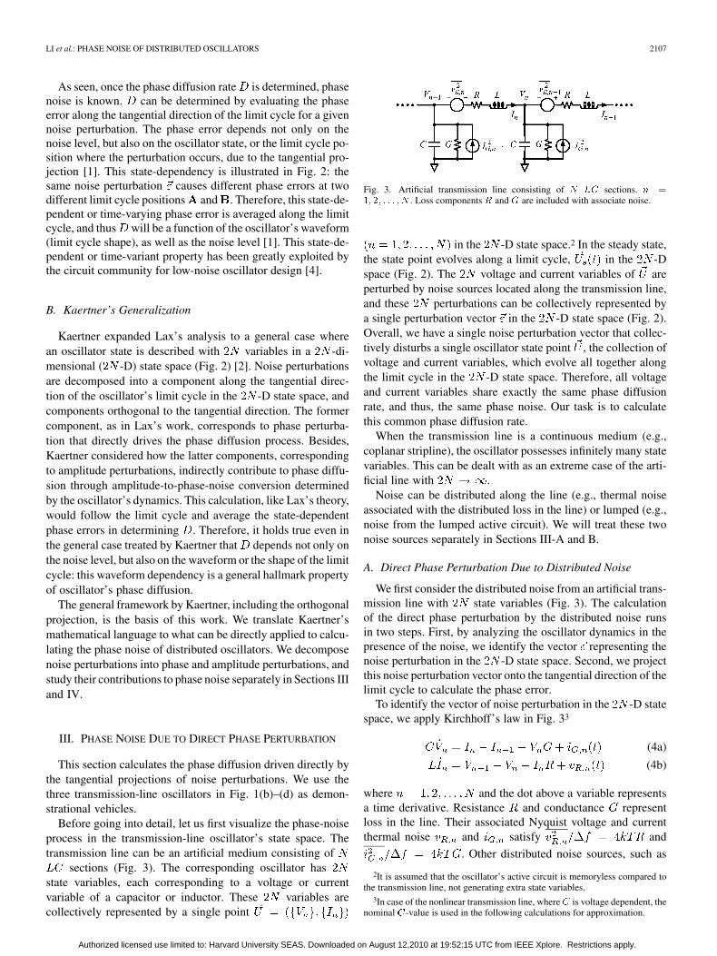
Fig. 2. Oscillator’s limit cycle in �� -D state space. For illustrative purposes,we only show two axes.

deal with noise sources, as in [3], which is another work byKaertner, extending his original work [2] to include the effect of

noise.Section II reviews the fundamental theories of phase noise by

Lax [1] and Kaertner [2]. Section III analyzes direct phase per-turbations and their effect on phase noise. Section IV examinesindirect phase perturbations caused by amplitude-to-phase errorconversion, and their effect on phase noise. Sections V and VIpresent measurements and their analysis.

II. PHASE-NOISE FUNDAMENTALS: REVIEW OF LAX’S AND

KAERTNER’S WORKS

A. Lax’s Fundamental Theory of Phase Noise

The essence of Lax’s work [1] may be understood as follows.Consider an oscillator [see Fig. 1(a)]. The voltage acrossand the current in the tank represent the oscillator’s state.The steady-state oscillation follows a closed-loop trajectory, orlimit cycle, in the 2-D – state space (Fig. 2 with ).Noise perturbs the oscillation, causing amplitude and phase er-rors. The amplitude error that puts oscillation off the limit cycleis constantly corrected by the oscillator’s tendency to return toits limit cycle. In contrast, the phase error on the limit cyclealong its tangential direction accumulates without bound for nomechanism to reset the phase exists. In other words, the phaseundergoes a diffusion along the limit cycle. Due to this phasediffusion, the oscillator’s output spectrum is broadened aroundthe oscillation frequency, causing phase noise.

Mathematically, in the presence of only white noise, the phasediffusion so occurs that the variance of the phase of the oscil-lation grows linearly with time

(1)

where is the phase diffusion rate. This leads to the well-known Lorentzian phase noise

(2)

and the behavior for

(3)

which is familiar from Leeson’s paper [22].


LI et al.: PHASE NOISE OF DISTRIBUTED OSCILLATORS 2107

As seen, once the phase diffusion rate is determined, phasenoise is known. can be determined by evaluating the phaseerror along the tangential direction of the limit cycle for a givennoise perturbation. The phase error depends not only on thenoise level, but also on the oscillator state, or the limit cycle po-sition where the perturbation occurs, due to the tangential pro-jection [1]. This state-dependency is illustrated in Fig. 2: thesame noise perturbation causes different phase errors at twodifferent limit cycle positions and . Therefore, this state-de-pendent or time-varying phase error is averaged along the limitcycle, and thus will be a function of the oscillator’s waveform(limit cycle shape), as well as the noise level [1]. This state-de-pendent or time-variant property has been greatly exploited bythe circuit community for low-noise oscillator design [4].

B. Kaertner’s Generalization

Kaertner expanded Lax’s analysis to a general case wherean oscillator state is described with variables in a -di-mensional ( -D) state space (Fig. 2) [2]. Noise perturbationsare decomposed into a component along the tangential direc-tion of the oscillator’s limit cycle in the -D state space, andcomponents orthogonal to the tangential direction. The formercomponent, as in Lax’s work, corresponds to phase perturba-tion that directly drives the phase diffusion process. Besides,Kaertner considered how the latter components, correspondingto amplitude perturbations, indirectly contribute to phase diffu-sion through amplitude-to-phase-noise conversion determinedby the oscillator’s dynamics. This calculation, like Lax’s theory,would follow the limit cycle and average the state-dependentphase errors in determining . Therefore, it holds true even inthe general case treated by Kaertner that depends not only onthe noise level, but also on the waveform or the shape of the limitcycle: this waveform dependency is a general hallmark propertyof oscillator’s phase diffusion.

The general framework by Kaertner, including the orthogonalprojection, is the basis of this work. We translate Kaertner’smathematical language to what can be directly applied to calcu-lating the phase noise of distributed oscillators. We decomposenoise perturbations into phase and amplitude perturbations, andstudy their contributions to phase noise separately in Sections IIIand IV.

III. PHASE NOISE DUE TO DIRECT PHASE PERTURBATION

This section calculates the phase diffusion driven directly bythe tangential projections of noise perturbations. We use thethree transmission-line oscillators in Fig. 1(b)–(d) as demon-strational vehicles.

Before going into detail, let us first visualize the phase-noiseprocess in the transmission-line oscillator’s state space. Thetransmission line can be an artificial medium consisting of

sections (Fig. 3). The corresponding oscillator hasstate variables, each corresponding to a voltage or currentvariable of a capacitor or inductor. These variables arecollectively represented by a single point

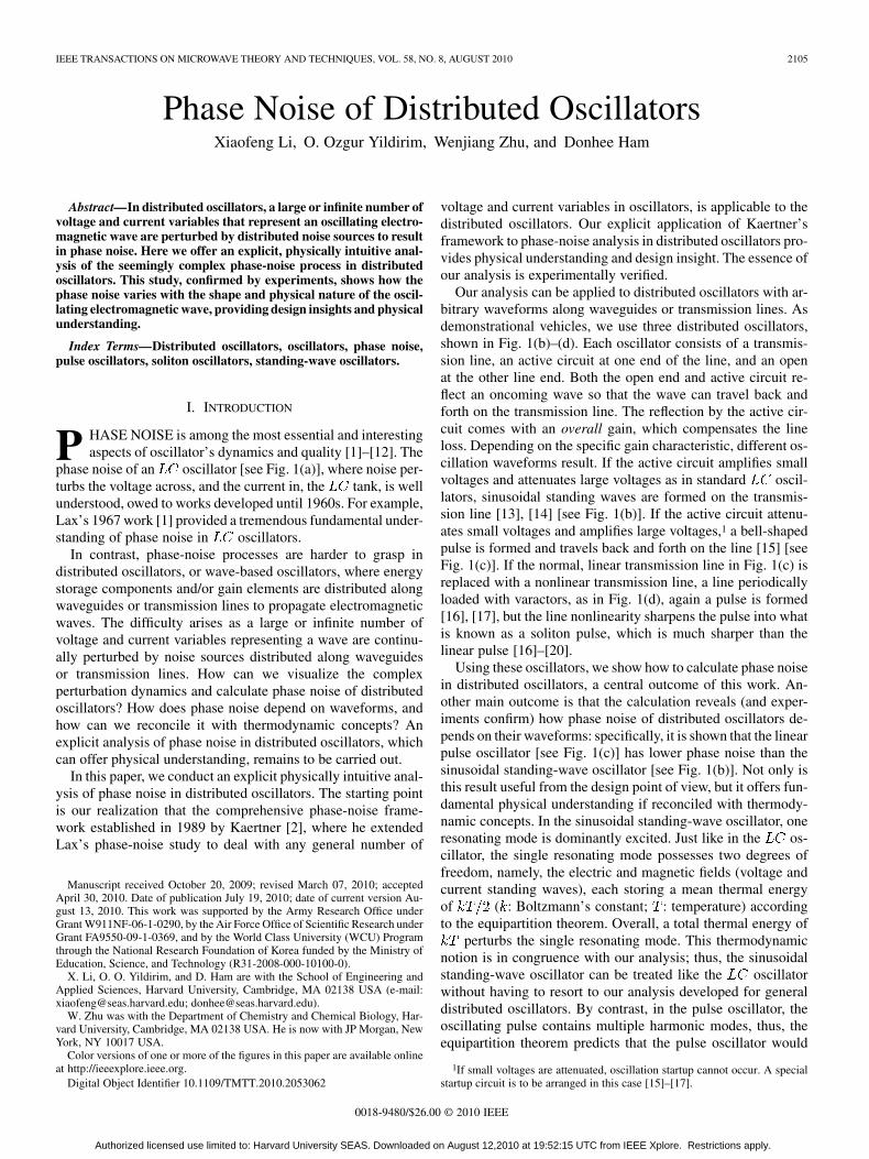
Fig. 3. Artificial transmission line consisting of � �� sections. � �

�� . Loss components � and � are included with associate noise.

in the -D state space.2 In the steady state,the state point evolves along a limit cycle, in the -Dspace (Fig. 2). The voltage and current variables of areperturbed by noise sources located along the transmission line,and these perturbations can be collectively represented bya single perturbation vector in the -D state space (Fig. 2).Overall, we have a single noise perturbation vector that collec-tively disturbs a single oscillator state point , the collection ofvoltage and current variables, which evolve all together alongthe limit cycle in the -D state space. Therefore, all voltageand current variables share exactly the same phase diffusionrate, and thus, the same phase noise. Our task is to calculatethis common phase diffusion rate.

When the transmission line is a continuous medium (e.g.,coplanar stripline), the oscillator possesses infinitely many statevariables. This can be dealt with as an extreme case of the arti-ficial line with .

Noise can be distributed along the line (e.g., thermal noiseassociated with the distributed loss in the line) or lumped (e.g.,noise from the lumped active circuit). We will treat these twonoise sources separately in Sections III-A and B.

A. Direct Phase Perturbation Due to Distributed Noise

We first consider the distributed noise from an artificial trans-mission line with state variables (Fig. 3). The calculationof the direct phase perturbation by the distributed noise runsin two steps. First, by analyzing the oscillator dynamics in thepresence of the noise, we identify the vector representing thenoise perturbation in the -D state space. Second, we projectthis noise perturbation vector onto the tangential direction of thelimit cycle to calculate the phase error.

To identify the vector of noise perturbation in the -D statespace, we apply Kirchhoff’s law in Fig. 33

(4a)

(4b)

where and the dot above a variable representsa time derivative. Resistance and conductance representloss in the line. Their associated Nyquist voltage and currentthermal noise and satisfy and

. Other distributed noise sources, such as

2It is assumed that the oscillator’s active circuit is memoryless compared tothe transmission line, not generating extra state variables.

3In case of the nonlinear transmission line, where� is voltage dependent, thenominal �-value is used in the following calculations for approximation.



those from distributed gain elements [21], if any, can be simi-larly modeled.

Change of variables, , , andwith an impedance-unit parameter renders and

dimensionless, and with the dimension of voltage. Withthe new variables, we rewrite (4) into

(5a)

(5b)

where and are rescalednoise terms that are independent Gaussian random variableswith zero mean and variance

[23]. Equation (5) identifies a random vectoras the noise perturbation vector during

the time interval . Also note that (5) treats voltage andcurrent variables symmetrically, or, in the equal unit, thanks tothe change of variable, .

Now resorting to Kaertner’s scheme [2], we project ontothe tangential direction of the limit cycle, or the direction ofmotion in the state space, which is defined by the state-space

velocity (Fig. 2). The inner product between and the unit

vector is the perturbation along the direction of motion.Division of this tangential perturbation by the magnitude of the

velocity yields the timing error , which is converted tothe phase error using , where is the oscillationfrequency.4 In sum,

(6)

As stated earlier, Kaertner derived a more general expressionfor the phase error using the tangential projection [2], and (6)is an explicit reduction of Kaertner’s expression, suitable forthe distributed oscillators. Since and are independentGaussian random variables with zero mean, is also Gaussianwith zero mean, and its variance is given by

(7)

Since the phase error must accumulate, growing its variance lin-early with time, (7) can be directly compared with the phase dif-fusion model (1) to find the phase diffusion rate

(8)

Since and are periodic functions of time, above isan instantaneous rate at a given time, and it varies periodicallywith time. This is because the size of the phase error even for afixed noise vector depends on the state of oscillation (wherethe state lies on the limit cycle), as indicated by (6), as illus-trated in Fig. 2, and as mentioned as a hallmark property of theoscillator phase diffusion [1], [2] in Section II. The periodically

4The detailed projection procedure up to this part of the present paragraph isgenerally captured in (16) and (23b) in Kaertner’s paper [2].

varying diffusion rate is usually time averaged over one oscilla-tion period to yield a constant diffusion rate, which matters overa long run

(9)

where represents the time average. This concludes our cal-culation of the direct phase perturbation and the resulting phasediffusion rate, arising from the distributed noise in the artificialtransmission line.

In the case of a continuous transmission line wherewith infinitesimally small sections, the phase diffusion ratecan be directly obtained from (9) by replacing the summationswith integrals and replacing , ,and with their values per unit length, , , , and (

, , , , )

(10)

where is the spatial coordinate along the line, is the partialtime derivative, and is the wave velocity on the line

(not to be confused with the state-space velocity ).Note that the time-averaged terms in (9) and (10) depend

on the shape of the limit cycle or the oscillating waveform,which originates from the state dependency of the phase error[1], [2]. Therefore, distributed oscillators with differing oscil-lating waveforms will exhibit different phase noise. To see thisconcretely and to interpret the waveform dependency in ther-modynamic terms, we now apply (9) or (10) to the three trans-mission-line oscillators [see Fig. 1(b)–(d)], but we start with alumped oscillator.

1) Lumped oscillator, Fig. 1(a): The voltage and currentin the tank of an almost sinusoidal oscillator are givenby and . Pluggingthese into (9) with , while only taking into account

with to model a parallel loss in the tank, we obtain

(11)

where is the total oscillation energy stored inthe tank and is the tank’s quality factor. Thisagrees with Lax’s work [1], and can be directly convertedto the well-known Leeson’s formula [22]. Note thatis the total thermal energy in the tank (corresponding tonoise) because and each stores a mean thermal energyof according to the equipartition theorem. The ratioof the thermal energy to the oscillation energy is thenoise-to-signal ratio.

2) Sinusoidal standing-wave oscillator, Fig. 1(b): Voltageand current standing waves in a continuous trans-mission line are and

where is thewavenumber. Plugging these into (10) and performing theintegrals over the line length , we find

(12)



where is the total energy stored in the trans-mission line, and is the quality factorof the line. Note that the phase diffusion rate of the si-nusoidal standing-wave oscillator above conforms to thatof the lumped oscillator in (11). This is expected andcan be understood in the Fourier domain: although the dis-tributed voltage and current variables in the transmissionline correspond to a large (or infinite) number of degreesof freedom in general, in the sinusoidal standing-wave os-cillator, only one resonance mode of the transmission lineis effectively excited. Like an tank, this resonancemode possesses only two degrees of freedom, namely, theelectric and magnetic fields (voltage and current standingwaves), each storing a mean thermal energy of . Itis then possible to treat sinusoidal standing-wave oscilla-tors effectively as lumped oscillators. In fact, using theFourier amplitudes as state variables, the dynamical equa-tions of standing-wave oscillators can be reduced to thoseof lumped oscillators. Such reduction was already car-ried out in the early stage of the phase-noise study formasers and lasers, whose microwave/optical cavities areindeed distributed waveguides that support microwave/op-tical standing waves [24]. The foregoing discussion maylead the reader to doubting the usefulness of our analysis.However, as we will show right below that this thermody-namic argument in the Fourier domain fails in the case ofpulse oscillators, and our analysis becomes necessary.

3) Linear and soliton pulse oscillators, Fig. 1(c) and (d): Thebell-shaped pulse in both linear and soliton pulse oscilla-tors may be described by the same functional form

with a full spatial width at halfmaximum , although the soliton pulse tendsto be sharper (larger ). Therefore, their phase diffusionrates can be calculated together using (10). Since the pulsetypically spans a length much shorter than the total lengthof the line, we can replace the integrals over the line length

in (10) with integrals over the entire -axis,5 i.e.,

(13)

to obtain

(14)

where is the total energy carried by thepulse. Equation (14) shows that phase noise of the pulseoscillator improves as the pulse gets sharper, a clear man-ifestation of the waveform dependency of captured bythe shape factor (time-averaged term) in (10). This can bephysically understood in time domain: noise perturbationgenerated at position affects the oscillator’s phase or thetiming of the pulse only when the pulse passes through thepoint. Its chance to enter the phase-noise process thus be-comes smaller as the pulsewidth decreases, yielding lower

5When the pulse reflects at the line ends, the instantaneous phase diffusionrate �� can be slightly modified due to superposition of the incident and re-flected pulses. The result after time averaging, however, remains unaltered.

and better phase noise. Since is approxi-mately the number of excited harmonic modes that consti-tute the pulse, (14) may be expressed as

. Had we treated the problem in theFourier domain assuming that the modes were indepen-dent of one another, each mode would store a thermal en-ergy of according to the equipartition theorem, and

would result. This, however,is an incorrect result, larger than the true value above bya factor of . The Fourier domain analysis fails becausethe harmonic modes are not independent, as their relativephases are coupled (or mode-locked) together. This consid-eration reveals the usefulness and necessity of our analysisin dealing with pulse oscillators.

Now let us compare the phase diffusion rate of the sinusoidalstanding-wave oscillator, (12), and that of the pulse oscillator,(14). Their evident difference is again the indication of the wave-form dependency of . If the standing-wave oscillator and pulseoscillator have the same amplitude for the same noise level, wehave

(15)

If the two oscillators have the same power dissipation for thesame noise level, we have

(16)

Therefore, for a very sharp pulse, .This physically makes sense as explained above, i.e., noise atany given point on the transmission line has less chance to par-ticipate in the phase-noise process for a spatially localized pulsethan for a standing wave spread over the transmission line, thus,the pulse oscillator is to have lower phase noise than the sinu-soidal standing-wave oscillator. Also we note once again that theFourier domain argument using the equipartition theorem wouldpredict an opposite and wrong result, i.e., higher phase noise forthe pulse oscillator that has a larger number of harmonic modesthan the sinusoidal standing-wave oscillator. Since the harmonicmodes in the pulse oscillator are inter-coupled, the equipartitiontheorem cannot be applied to the pulse oscillator, as discussedabove.

B. Direct Phase Perturbation Due to Lumped Noise

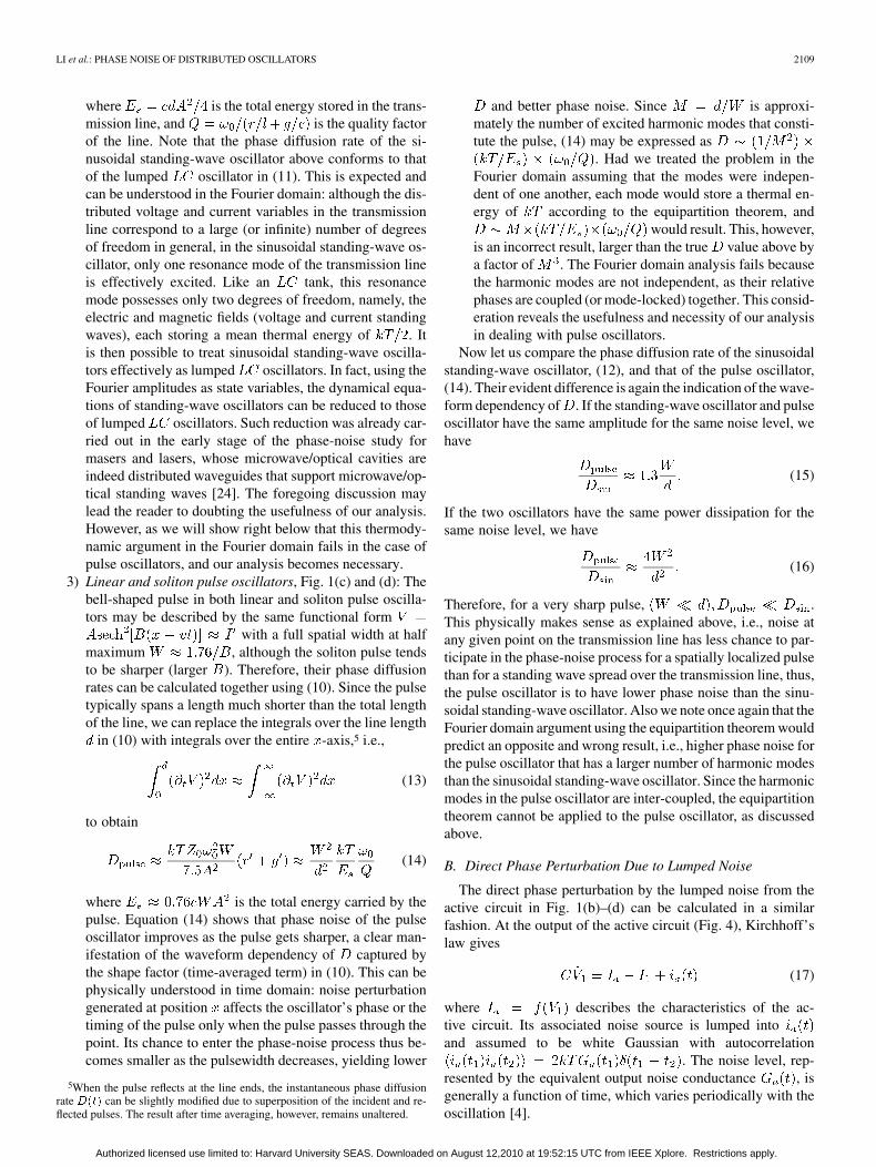
The direct phase perturbation by the lumped noise from theactive circuit in Fig. 1(b)–(d) can be calculated in a similarfashion. At the output of the active circuit (Fig. 4), Kirchhoff’slaw gives

(17)

where describes the characteristics of the ac-tive circuit. Its associated noise source is lumped intoand assumed to be white Gaussian with autocorrelation

. The noise level, rep-resented by the equivalent output noise conductance , isgenerally a function of time, which varies periodically with theoscillation [4].



Fig. 4. Circuit model for the active circuit with lumped noise.

As in Section III-A, using change of variables and, we rewrite (14) into

(18)

where is a Gaussian random variable with zeromean and variance . This equation identi-fies as a noise perturbation vector inthe -D state space. By projecting along the tangential di-rection of the limit cycle and following the same procedure inSection III-A, we obtain the following phase diffusion rate dueto the direct phase perturbation by the lumped noise for the ar-tificial transmission line case:

(19)

In the case of continuous transmission line, it becomes

(20)

The time-averaged terms in (19) and (20) once again ex-hibit the waveform dependency, as a consequence of the statedependency of the phase error. We again apply these resultsto the distributed oscillators in Fig. 1(b)–(d). Evaluation of(19) and (20) requires knowledge of the specific form of thetime-varying noise level . In each of our experimentalcircuits corresponding to Fig. 1(b)–(d), is almost aconstant (Section V). Therefore, a constant is used in thefollowing calculations.

1) Sinusoidal standing-wave oscillator, Fig. 1(b):and

in (20) yield

(21)

2) Linear and soliton pulse oscillators, Fig. 1(c) and (d):At the active circuit end of the line, an incident pulseis superposed with a reflected pulse. The joint voltageamplitude is about twice the incident pulse amplitude, or

, assuming linear superposition.6

Using this and (13) in (20), we obtain

(22)

6In the soliton oscillator case, � �� may slightly differ from the linear su-perposition due to the nonlinear interaction between the oncoming and reflectedpulses, but we do not expect this to significantly change the result.

Comparing (21) with (22), we find

(23)

if the standing-wave and pulse oscillators have the same ampli-tude for the same lumped noise level, and

(24)

if they have the same power dissipation for the same lumpednoise level. These results are exactly the same as in the case ofdistributed noise perturbation: (15) and (16). The results againindicate that a sharper pulse experiences the lumped noise at

for a shorter period of time, thus yielding a slower phasediffusion.

We point out that even in the foregoing case of lumped noise,the analysis has still dealt with the distributed nature: the largeset of voltage and current variables representing the oscillatingelectromagnetic wave are distributed along the transmissionline, even if the noise source is lumped. The analysis has shownhow a perturbation even at one fixed point affects the collectiveoscillation of the entire distributed system.

Thus far we have considered only the direct phase perturba-tions along the tangential directions of the limit cycle, while notaddressing the effect of the amplitude perturbation. As shownby Kaertner, the amplitude perturbation can contribute substan-tially to phase diffusion through amplitude-to-phase-noise con-version in certain oscillators [2]. This effect is not of great im-portance in the standing-wave and linear pulse oscillators for theoscillation frequency of the linear transmission line with rea-sonably high7 is essentially independent of oscillation ampli-tude. Therefore, the analysis above is sufficient for the standing-wave and linear pulse oscillators, and it remains valid that thelatter has less phase noise than the former. In contrast, in thesoliton pulse oscillator, the amplitude perturbation will translateto timing perturbations through soliton’s amplitude-dependentpropagation speed in the nonlinear transmission line, which cancontribute significantly to phase noise. We now turn to this issuefor the soliton oscillator.

IV. AMPLITUDE PERTURBATION AND ITS PHASE-NOISE EFFECT

IN SOLITON OSCILLATORS

This section examines how amplitude perturbation con-tributes to phase noise in the soliton oscillator throughamplitude-to-phase error conversion. We again use Kaertner’sorthogonal projection scheme, but we do not carry it out in fullto determine the exact amplitude-to-phase error conversion,which requires diagonalizing large matrices corresponding tooscillator’s dynamical equations linearized in proximity ofits limit cycle. Instead, we evaluate the effect by devising anintuitive phenomenological approach that captures the essenceof amplitude-to-phase error conversion in the soliton oscillator.

A soliton pulse propagating in a nonlinear transmission linecan be described as ,

7As seen in Section VI, measured � is about 100.



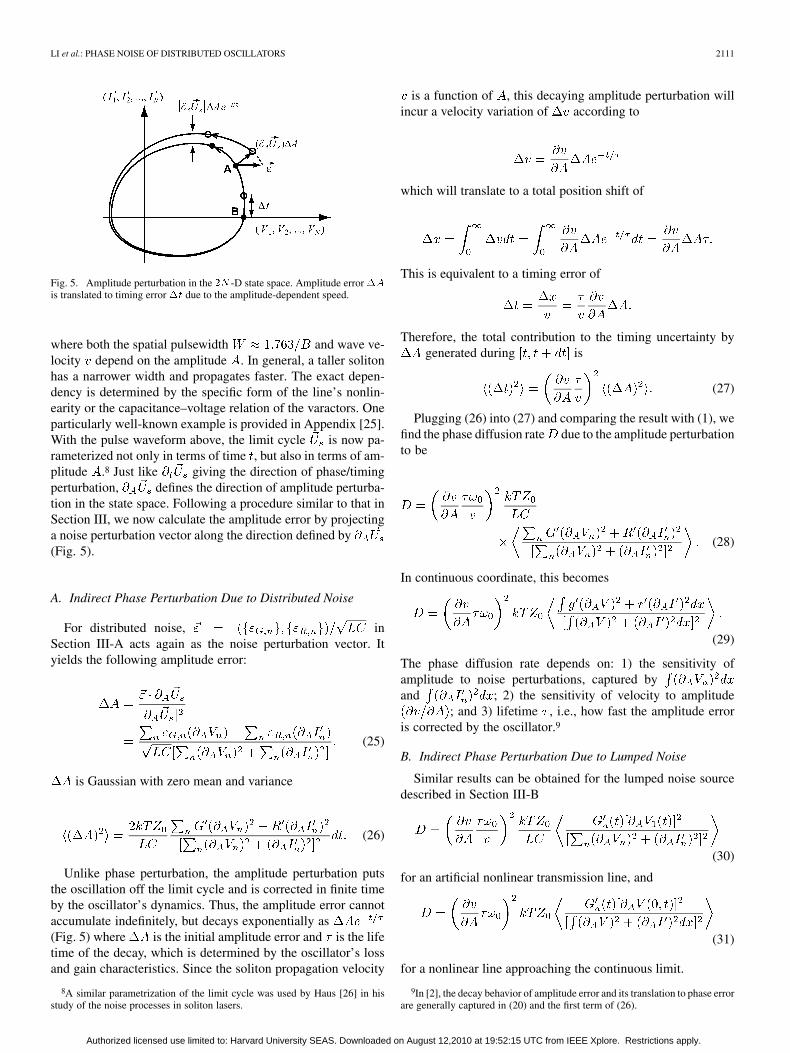
Fig. 5. Amplitude perturbation in the �� -D state space. Amplitude error��is translated to timing error�� due to the amplitude-dependent speed.

where both the spatial pulsewidth and wave ve-locity depend on the amplitude . In general, a taller solitonhas a narrower width and propagates faster. The exact depen-dency is determined by the specific form of the line’s nonlin-earity or the capacitance–voltage relation of the varactors. Oneparticularly well-known example is provided in Appendix [25].With the pulse waveform above, the limit cycle is now pa-rameterized not only in terms of time , but also in terms of am-plitude .8 Just like giving the direction of phase/timingperturbation, defines the direction of amplitude perturba-tion in the state space. Following a procedure similar to that inSection III, we now calculate the amplitude error by projectinga noise perturbation vector along the direction defined by(Fig. 5).

A. Indirect Phase Perturbation Due to Distributed Noise

For distributed noise, inSection III-A acts again as the noise perturbation vector. Ityields the following amplitude error:

(25)

is Gaussian with zero mean and variance

(26)

Unlike phase perturbation, the amplitude perturbation putsthe oscillation off the limit cycle and is corrected in finite timeby the oscillator’s dynamics. Thus, the amplitude error cannotaccumulate indefinitely, but decays exponentially as(Fig. 5) where is the initial amplitude error and is the lifetime of the decay, which is determined by the oscillator’s lossand gain characteristics. Since the soliton propagation velocity

8A similar parametrization of the limit cycle was used by Haus [26] in hisstudy of the noise processes in soliton lasers.

is a function of , this decaying amplitude perturbation willincur a velocity variation of according to

which will translate to a total position shift of

This is equivalent to a timing error of

Therefore, the total contribution to the timing uncertainty bygenerated during is

(27)

Plugging (26) into (27) and comparing the result with (1), wefind the phase diffusion rate due to the amplitude perturbationto be

(28)

In continuous coordinate, this becomes

(29)

The phase diffusion rate depends on: 1) the sensitivity ofamplitude to noise perturbations, captured byand ; 2) the sensitivity of velocity to amplitude

; and 3) lifetime , i.e., how fast the amplitude erroris corrected by the oscillator.9

B. Indirect Phase Perturbation Due to Lumped Noise

Similar results can be obtained for the lumped noise sourcedescribed in Section III-B

(30)

for an artificial nonlinear transmission line, and

(31)

for a nonlinear line approaching the continuous limit.

9In [2], the decay behavior of amplitude error and its translation to phase errorare generally captured in (20) and the first term of (26).



C. Indirect Versus Direct Phase Perturbations

Let us first note that the total phase diffusion rate in a solitonoscillator is a sum of caused by direct phase perturbationsand induced by amplitude perturbations. This simple addi-tion is possible because the amplitude perturbation [e.g., (25)]and the phase perturbation [e.g., (6)] are orthogonal or uncor-related to each other. This orthogonality can be checked bynoticing that and in (25) are even functions of ,whereas and in (6) are odd.

Given this simple addition, we may directly compareand to see which process contributes more to the

total phase diffusion rate. For a concrete comparison, weuse the well-known soliton model that takes a waveform of

with specific expressionsfor and found in the Appendix. With this soliton,(29) yields

(32)

for distributed noise sources. Comparing this with of (14)that is caused by the same distributed noise sources, we have

(33)

Exactly the same relationship holds in the case of lumped noiseperturbations, according to (20) and (31) if is a constant,which is the case in our experiment. As seen, the ratio dependslargely on the velocity-amplitude relation and the life time ofamplitude errors. can be far larger than , which is thecase in our experiment (see Section V).

V. EXPERIMENT

A. Oscillator Prototypes

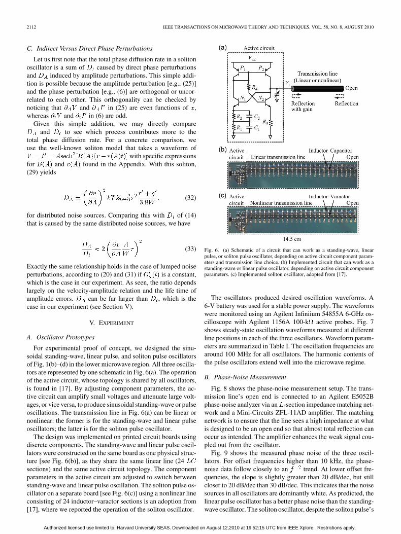
For experimental proof of concept, we designed the sinu-soidal standing-wave, linear pulse, and soliton pulse oscillatorsof Fig. 1(b)–(d) in the lower microwave region. All three oscilla-tors are represented by one schematic in Fig. 6(a). The operationof the active circuit, whose topology is shared by all oscillators,is found in [17]. By adjusting component parameters, the ac-tive circuit can amplify small voltages and attenuate large volt-ages, or vice versa, to produce sinusoidal standing-wave or pulseoscillations. The transmission line in Fig. 6(a) can be linear ornonlinear: the former is for the standing-wave and linear pulseoscillators; the latter is for the soliton pulse oscillator.

The design was implemented on printed circuit boards usingdiscrete components. The standing-wave and linear pulse oscil-lators were constructed on the same board as one physical struc-ture [see Fig. 6(b)], as they share the same linear line (24sections) and the same active circuit topology. The componentparameters in the active circuit are adjusted to switch betweenstanding-wave and linear pulse oscillation. The soliton pulse os-cillator on a separate board [see Fig. 6(c)] using a nonlinear lineconsisting of 24 inductor–varactor sections is an adoption from[17], where we reported the operation of the soliton oscillator.

Fig. 6. (a) Schematic of a circuit that can work as a standing-wave, linearpulse, or soliton pulse oscillator, depending on active circuit component param-eters and transmission line choice. (b) Implemented circuit that can work as astanding-wave or linear pulse oscillator, depending on active circuit componentparameters. (c) Implemented soliton oscillator, adopted from [17].

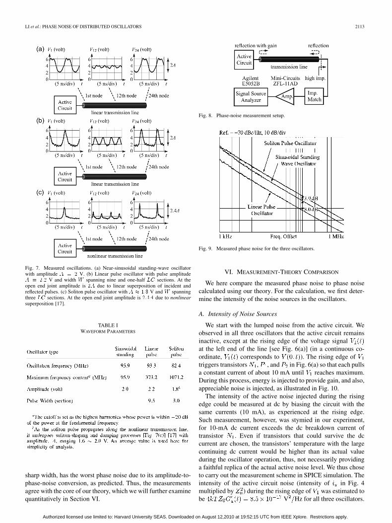
The oscillators produced desired oscillation waveforms. A6-V battery was used for a stable power supply. The waveformswere monitored using an Agilent Infiniium 54855A 6-GHz os-cilloscope with Agilent 1156A 100-k active probes. Fig. 7shows steady-state oscillation waveforms measured at differentline positions in each of the three oscillators. Waveform param-eters are summarized in Table I. The oscillation frequencies arearound 100 MHz for all oscillators. The harmonic contents ofthe pulse oscillators extend well into the microwave regime.

B. Phase-Noise Measurement

Fig. 8 shows the phase-noise measurement setup. The trans-mission line’s open end is connected to an Agilent E5052Bphase-noise analyzer via an -section impedance matching net-work and a Mini-Circuits ZFL-11AD amplifier. The matchingnetwork is to ensure that the line sees a high impedance at whatis designed to be an open end so that almost total reflection canoccur as intended. The amplifier enhances the weak signal cou-pled out from the oscillator.

Fig. 9 shows the measured phase noise of the three oscil-lators. For offset frequencies higher than 10 kHz, the phase-noise data follow closely to an trend. At lower offset fre-quencies, the slope is slightly greater than 20 dB/dec, but stillcloser to 20 dB/dec than 30 dB/dec. This indicates that the noisesources in all oscillators are dominantly white. As predicted, thelinear pulse oscillator has a better phase noise than the standing-wave oscillator. The soliton oscillator, despite the soliton pulse’s



Fig. 7. Measured oscillations. (a) Near-sinusoidal standing-wave oscillatorwith amplitude � � � V. (b) Linear pulse oscillator with pulse amplitude� � �� V and width � spanning nine and one-half �� sections. At theopen end joint amplitude is �� due to linear superposition of incident andreflected pulses. (c) Soliton pulse oscillator with � � �� V and � spanningthree �� sections. At the open end joint amplitude is �� due to nonlinearsuperposition [17].

TABLE IWAVEFORM PARAMETERS

sharp width, has the worst phase noise due to its amplitude-to-phase-noise conversion, as predicted. Thus, the measurementsagree with the core of our theory, which we will further examinequantitatively in Section VI.

Fig. 8. Phase-noise measurement setup.

Fig. 9. Measured phase noise for the three oscillators.

VI. MEASUREMENT-THEORY COMPARISON

We here compare the measured phase noise to phase noisecalculated using our theory. For the calculation, we first deter-mine the intensity of the noise sources in the oscillators.

A. Intensity of Noise Sources

We start with the lumped noise from the active circuit. Weobserved in all three oscillators that the active circuit remainsinactive, except at the rising edge of the voltage signalat the left end of the line [see Fig. 6(a)] (in a continuous co-ordinate, corresponds to ). The rising edge oftriggers transistors , , and in Fig. 6(a) so that each pullsa constant current of about 10 mA until reaches maximum.During this process, energy is injected to provide gain, and also,appreciable noise is injected, as illustrated in Fig. 10.

The intensity of the active noise injected during the risingedge could be measured at dc by biasing the circuit with thesame currents (10 mA), as experienced at the rising edge.Such measurement, however, was stymied in our experiment,for 10-mA dc current exceeds the dc breakdown current oftransistor . Even if transistors that could survive the dccurrent are chosen, the transistors’ temperature with the largecontinuing dc current would be higher than its actual valueduring the oscillator operation, thus, not necessarily providinga faithful replica of the actual active noise level. We thus choseto carry out the measurement scheme in SPICE simulation. Theintensity of the active circuit noise (intensity of in Fig. 4multiplied by ) during the rising edge of was estimated tobe V Hz for all three oscillators.



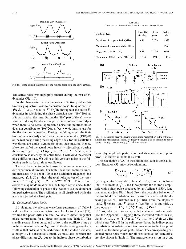
Fig. 10. Time-domain illustration of the lumped noise from the active circuits.

The active noise was negligibly smaller during the rest ofdynamics (Fig. 10).

For the phase-noise calculation, we can effectively reduce thistime-varying active noise to a constant noise. Imagine we use

V Hz throughout the entiredynamics in calculating the phase diffusion rate [(19)/(20)], asif it persisted all the time. During the “flat” part of the wave-form, i.e., during the absence of pulse events or transition edgeswhen there is no actual appreciable noise, the fictitious noisedoes not contribute to (19)/(20), as , thus, its use forthe flat duration is justified. During the falling edges, the ficti-tious noise spuriously contributes the same amount to (19)/(20)as the real noise during the rising edges does, for the oscillationwaveforms are almost symmetric about their maxima. Hence,if we use half of the actual noise intensity injected only duringthe rising edge, i.e., V Hz, as aconstant noise intensity the entire time, it will yield the correctphase diffusion rate. We will use this constant noise in the fol-lowing analysis for all three oscillators.

The distributed noise in the transmission line is far smaller inour experimental circuits. For both linear and nonlinear lines,the measured is about 100 at the oscillation frequency andmeasured is 50 , thus, the total noise power of the lossylines is V Hz. This is threeorders of magnitude smaller than the lumped active noise. In thefollowing calculation of phase noise, we only use the dominantlumped active noise. The oscillation is still distributed while thenoise is injected at a fixed point.

B. Calculated Phase Noise

By plugging the relevant waveform parameters of Table Iand the effective constant active noise level into (21) and (22),we find the phase diffusion rate, , due to direct tangentialphase perturbation, for all three oscillators (see Table II). Thestanding-wave, linear pulse, and soliton pulse oscillators line upin the decreasing order of , owed to the decreasing waveformwidth in that order, as explained earlier. In the soliton oscillator,although is substantially small, we must also consider thephase diffusion rate due to the indirect phase perturbation

TABLE IICALCULATED PHASE DIFFUSION RATES AND PHASE NOISE

Fig. 11. Measured decay behavior of amplitude perturbation in the soliton os-cillator. (a) Measurement setup. (b) Decay behavior after an amplitude pertur-bation ��. (c) � extraction. (d) �� extraction.

caused by amplitude perturbation and its conversion to phaseerror. It is shown in Table II as well.

The calculation of in the soliton oscillator is done as fol-lows. Equation (33) may be rewritten into

(34)

by using soliton’s round-trip time in the nonlinearline. To estimate and , we perturb the soliton’s ampli-tude with a short pulse produced by an Agilent 81150A func-tion generator [see Fig. 11(a)]. From the decaying behavior ofthe amplitude perturbation, we measure and of the de-caying pulse, as illustrated in Fig. 11(b). From the slopes of

versus and versus [see Fig. 11(c) and (d)], wethen obtain and

ns, which are consistent with the standard soliton model(see the Appendix). Plugging these measured values in (34)yields Hz,which enter Table II. In the soliton oscillator, the indirect phaseperturbation contributes about ten times more to the total phasenoise than the direct phase perturbation. The corresponding cal-culated phase-noise values for all oscillators at 100-kHz offsetare also shown in Table II. The measurement errors in and



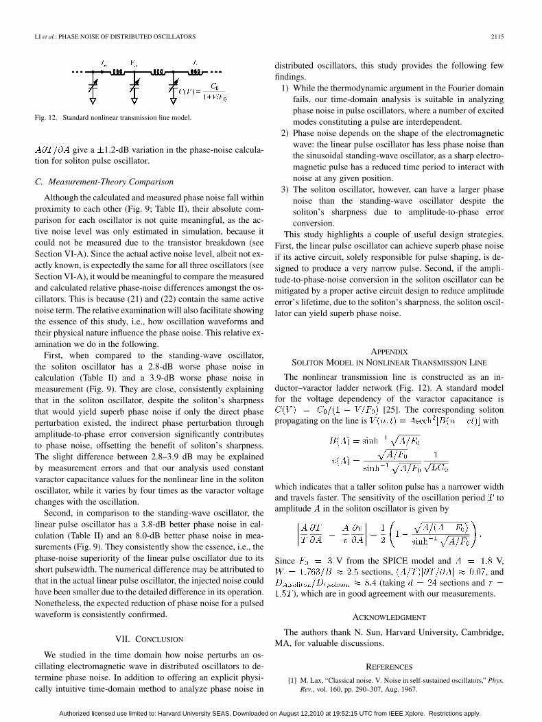
Fig. 12. Standard nonlinear transmission line model.

give a 1.2-dB variation in the phase-noise calcula-tion for soliton pulse oscillator.

C. Measurement-Theory Comparison

Although the calculated and measured phase noise fall withinproximity to each other (Fig. 9; Table II), their absolute com-parison for each oscillator is not quite meaningful, as the ac-tive noise level was only estimated in simulation, because itcould not be measured due to the transistor breakdown (seeSection VI-A). Since the actual active noise level, albeit not ex-actly known, is expectedly the same for all three oscillators (seeSection VI-A), it would be meaningful to compare the measuredand calculated relative phase-noise differences amongst the os-cillators. This is because (21) and (22) contain the same activenoise term. The relative examination will also facilitate showingthe essence of this study, i.e., how oscillation waveforms andtheir physical nature influence the phase noise. This relative ex-amination we do in the following.

First, when compared to the standing-wave oscillator,the soliton oscillator has a 2.8-dB worse phase noise incalculation (Table II) and a 3.9-dB worse phase noise inmeasurement (Fig. 9). They are close, consistently explainingthat in the soliton oscillator, despite the soliton’s sharpnessthat would yield superb phase noise if only the direct phaseperturbation existed, the indirect phase perturbation throughamplitude-to-phase error conversion significantly contributesto phase noise, offsetting the benefit of soliton’s sharpness.The slight difference between 2.8–3.9 dB may be explainedby measurement errors and that our analysis used constantvaractor capacitance values for the nonlinear line in the solitonoscillator, while it varies by four times as the varactor voltagechanges with the oscillation.

Second, in comparison to the standing-wave oscillator, thelinear pulse oscillator has a 3.8-dB better phase noise in cal-culation (Table II) and an 8.0-dB better phase noise in mea-surements (Fig. 9). They consistently show the essence, i.e., thephase-noise superiority of the linear pulse oscillator due to itsshort pulsewidth. The numerical difference may be attributed tothat in the actual linear pulse oscillator, the injected noise couldhave been smaller due to the detailed difference in its operation.Nonetheless, the expected reduction of phase noise for a pulsedwaveform is consistently confirmed.

VII. CONCLUSION

We studied in the time domain how noise perturbs an os-cillating electromagnetic wave in distributed oscillators to de-termine phase noise. In addition to offering an explicit physi-cally intuitive time-domain method to analyze phase noise in

distributed oscillators, this study provides the following fewfindings.

1) While the thermodynamic argument in the Fourier domainfails, our time-domain analysis is suitable in analyzingphase noise in pulse oscillators, where a number of excitedmodes constituting a pulse are interdependent.

2) Phase noise depends on the shape of the electromagneticwave: the linear pulse oscillator has less phase noise thanthe sinusoidal standing-wave oscillator, as a sharp electro-magnetic pulse has a reduced time period to interact withnoise at any given position.

3) The soliton oscillator, however, can have a larger phasenoise than the standing-wave oscillator despite thesoliton’s sharpness due to amplitude-to-phase errorconversion.

This study highlights a couple of useful design strategies.First, the linear pulse oscillator can achieve superb phase noiseif its active circuit, solely responsible for pulse shaping, is de-signed to produce a very narrow pulse. Second, if the ampli-tude-to-phase-noise conversion in the soliton oscillator can bemitigated by a proper active circuit design to reduce amplitudeerror’s lifetime, due to the soliton’s sharpness, the soliton oscil-lator can yield superb phase noise.

APPENDIX

SOLITON MODEL IN NONLINEAR TRANSMISSION LINE

The nonlinear transmission line is constructed as an in-ductor–varactor ladder network (Fig. 12). A standard modelfor the voltage dependency of the varactor capacitance is

[25]. The corresponding solitonpropagating on the line is with

which indicates that a taller soliton pulse has a narrower widthand travels faster. The sensitivity of the oscillation period toamplitude in the soliton oscillator is given by

Since V from the SPICE model and V,sections, , and

(taking sections and), which are in good agreement with our measurements.

ACKNOWLEDGMENT

The authors thank N. Sun, Harvard University, Cambridge,MA, for valuable discussions.

REFERENCES

[1] M. Lax, “Classical noise. V. Noise in self-sustained oscillators,” Phys.Rev., vol. 160, pp. 290–307, Aug. 1967.



[2] F. X. Kaertner, “Determination of the correlation spectrum of oscilla-tors with low noise,” IEEE Trans. Microw. Theory Tech., vol. 37, no. 1,pp. 90–101, Jan. 1989.

[3] F. X. Kaertner, “Analysis of white and � noise in oscillators,” Int.J. Circuit Theory Appl., vol. 18, pp. 485–519, 1990.

[4] A. Hajimiri and T. H. Lee, “A general theory of phase noise in electricaloscillators,” IEEE J. Solid-State Circuits, vol. 33, no. 2, pp. 179–194,Feb. 1998.

[5] A. Demir, A. Mehrotra, and J. Roychowdhury, “Phase noise in oscil-lators: A unifying theory and numerical methods for characterization,”IEEE Trans. Circuits Syst. I, Fundam. Theory Appl., vol. 47, no. 5, pp.655–674, May 2000.

[6] A. Demir, “Phase noise and timing jitter in oscillators with colorednoise sources,” IEEE Trans. Circuits Syst. I, Fundam. Theory Appl.,vol. 49, no. 12, pp. 1782–1791, Dec. 2002.

[7] A. Suarez, S. Sancho, S. Ver Hoeye, and J. Portilla, “Analytical com-parison between time- and frequency-domain techniques for phase-noise analysis,” IEEE Trans. Microw. Theory Tech., vol. 50, no. 10,pp. 2353–2361, Oct. 2002.

[8] T. Djurhuus, V. Krozer, J. Vidkjaer, and T. K. Johansen, “Oscillatorphase noise: A geometrical approach,” IEEE Trans. Circuits Syst. I,Reg. Papers, vol. 56, no. 7, pp. 1373–1382, July 2009.

[9] A. Blaquiere, Nonlinear System Analysis. New York: Academic,1966.

[10] K. Kurokawa, An Introduction to the Theory of Microwave Circuits.New York: Academic, 1969.

[11] E. E. Hegazi, J. Rael, and A. Abidi, The Designer’s Guide to High-Purity Oscillators. Berlin, Germany: Springer, 2004.

[12] A. Suarez, Analysis and Design of Autonomous Microwave Circuits.New York: Wiley, 2009.

[13] F. O’Mahony, C. P. Yue, M. A. Horowitz, and S. S. Wong, “A 10-GHzglobal clock distribution using coupled standing-wave oscillators,”IEEE J. Solid-State Circuits, vol. 38, no. 11, pp. 1813–1820, Nov.2003.

[14] W. F. Andress and D. Ham, “Standing wave oscillators utilizing wave-adaptive tapered transmission lines,” IEEE J. Solid-State Circuits, vol.40, no. 3, pp. 638–651, Mar. 2005.

[15] L. A. Glasser and H. A. Haus, “Microwave mode locking at �-bandusing solid-state devices,” IEEE Trans. Microw. Theory Tech., vol.MTT-26, no. 2, pp. 62–69, Feb. 1978.

[16] D. Ricketts, X. Li, and D. Ham, “Electrical soliton oscillator,” IEEETrans. Microw. Theory Tech., vol. 54, no. 1, pp. 373–382, Jan. 2006.

[17] O. O. Yildirim, D. Ricketts, and D. Ham, “Reflection soliton oscillator,”IEEE Trans. Microw. Theory Tech., vol. 57, no. 10, pp. 2344–2353, Oct.2009.

[18] C. J. Madden, R. A. Marsland, M. J. W. Rodwell, D. M. Bloom, andY. C. Pao, “Hyperabrupt-doped GaAs nonlinear transmission line forpicosecond shock-wave generation,” Appl. Phys. Lett., vol. 54, no. 11,pp. 1019–1021, Mar. 1989.

[19] M. Case, M. Kamegawa, R. Y. Yu, M. J. W. Rodwell, and J. Franklin,“Impulse compression using soliton effects in a monolithic GaAs cir-cuit,” Appl. Phys. Lett., vol. 58, no. 2, pp. 173–175, Jan. 1991.

[20] K. S. Giboney, M. J. W. Rodwell, and J. E. Bowers, “Traveling-wavephotodetector theory,” IEEE Trans. Microw. Theory Tech., vol. 45, no.8, pp. 1310–1319, Aug. 1997.

[21] B. Kleveland, C. H. Diaz, D. Vook, L. Madden, T. H. Lee, and S.S. Wong, “Monolithic CMOS distributed amplifier and oscillator,” inIEEE Int. Solid-State Circuits Conf. Tech. Dig., Feb. 1999, pp. 70–71.

[22] D. B. Leeson, “A simple model of feedback oscillator noise spectrum,”Proc. IEEE, vol. 54, no. 2, pp. 329–330, Feb. 1966.

[23] J. A. Gubner, Probability and Random Processes for Electrical andComputer Engineers. Cambridge, MA: Cambridge Univ. Press,2006, pp. 453–459.

[24] M. Lax and W. H. Louisell, “Quantum noise IX: QuantumFokker–Planck solution for laser noise,” IEEE J. Quantum Elec-tron., vol. QE-3, no. 2, pp. 47–58, Feb. 1967.

[25] M. Toda, Nonlinear Waves and Solitons. Norwell, MA: Kluwer,1989.

[26] H. A. Haus and Y. Lai, “Quantum theory of soliton squeezing: A lin-earized approach,” J. Opt. Soc. Amer. B, Opt. Phys., vol. 7, no. 3, pp.386–392, Mar. 1990.

Xiaofeng Li was born in Luoyang, China. He re-ceived the B.S. degree in electrical engineering fromthe California Institute of Technology, Pasadena,in 2004, and is currently working toward the Ph.D.degree in electrical engineering from the Schoolof Engineering and Applied Sciences, HarvardUniversity, Cambridge, MA.

His research interests lie in the transformative areaof emerging circuits and devices in conjunction withstatistical physics, condensed matter physics, andmaterial sciences. His research includes nonlinear

electrical soliton oscillators, phase noise of self-sustained electrical oscillatorsand biological oscillators, and microfluidic stretchable electronics. He iscurrently conducting an experiment to study gigahertz–terahertz plasmonicwaves using 1-D nanoscale devices, and to demonstrate their engineering utilityin circuit applications.

Mr. Li was a Gold Medalist at the 29th International Physics Olympiad, Ice-land, 1998. He ranked first in the Boston Area Undergraduate Physics Compe-tition in both 2001 and 2002. He was also the recipient of the 2002 CaliforniaInstitute of Technology Henry Ford II Scholar Award, the 2004 Harvard Uni-versity Peirce Fellowship, and the 2005 Analog Devices Outstanding StudentDesigner Award.

O. Ozgur Yildirim received the B.S. and M.S. de-grees in electrical and electronics engineering fromMiddle East Technical University, Ankara, Turkey, in2004 and 2006, respectively, and is currently workingtoward the Ph.D. degree in electrical engineering andapplied physics at Harvard University, Cambridge,MA.

In the summers of 2002 and 2003, he waswith the Scientific and Research Council of Turkey(TUBITAK), Ankara, Turkey, where he was involvedwith the development of a dynamic power com-

pensation card and a field-programmable gate array (FPGA) for synchronousdynamic RAM interface. For his Master’s research, he was involved withthe development of on-chip readout electronics for uncooled microbolometerdetector arrays for infrared camera applications. His research interests includeultrafast and RF integrated circuits and devices, soliton and nonlinear waves andtheir utilization in electronic circuits, and nanoscale and terahertz electronics.

Mr. Yildirim was the recipient of the 2009 Analog Devices Outstanding Stu-dent Designer Award.

Wenjiang Zhu was born in Lanzhou, China. He re-ceived the B.S. degree in chemistry from Peking Uni-versity, Beijing, China, in 2002, the M.A. degree inchemistry from Princeton University, Princeton, NJ,in 2004, and the Ph.D. degree in chemistry from Har-vard University, Cambridge, MA, in 2008. He alsoreceived the A.M. degree in statistics from HarvardUniversity, Cambridge, MA, in 2008.

He is currently with JP Morgan, New York, NY.His scientific expertise lies in applying statistical andstochastic methods to a range of dynamical problems

in physics, biology, and finance.

Donhee Ham received the B.S. degree (summa cumlaude) in physics from Seoul National University,Seoul, Korea, in 1996, and the Ph.D. degree inelectrical engineering from the California Instituteof Technology, Pasadena, in 2002. His doctoralresearch examined the statistical physics of electricalcircuits.

He is currently the Gordon McKay Professorof Applied Physics and Electrical Engineering atHarvard University, Cambridge, MA, where he iswith the School of Engineering and Applied Sci-

ences. The intellectual focus of his research laboratory at Harvard Universityis electronic, electrochemical, and optical biomolecular analysis using siliconintegrated circuits and bottom-up nanoscale systems for biotechnology and



medicine; quantum plasmonic circuits using 1-D nanoscale devices; spin-basedquantum computing on silicon chips; and RF, analog, and mixed-signal inte-grated circuits. His research experiences include affiliations with the CaliforniaInstitute of Technology–Massachusetts Institute of Technology (MIT) LaserInterferometer Gravitational Wave Observatory (LIGO), the IBM T. J. WatsonResearch, and a visiting professorship with POSTECH. He was a coeditor ofCMOS Biotechnology (2007).

Dr. Ham is a member of the IEEE conference Technical Program Committeesincluding the IEEE International Solid-State Circuits Conference and the IEEEAsian Solid-State Circuits Conference, Advisory Board for the IEEE Interna-tional Symposium on Circuits and Systems, International Advisory Board forthe Institute for Nanodevice and Biosystems, and various U.S., Korea, and Japanindustry, government, and academic technical advisory positions on subjects in-cluding ultrafast electronics, science and technology at the nanoscale, and con-vergence of information technology and biotechnology. He was a guest editor

for the IEEE JOURNAL OF SOLID-STATE CIRCUITS. He received the ValedictorianPrize, the Presidential Prize, ranked top first across the Natural Science Col-lege of Seoul National University, and also the Physics Gold Medal from SeoulNational University. He was the recipient of the Charles Wilts Prize given forthe best doctoral dissertation in electrical engineering at the California Instituteof Technology. He was the recipient of the IBM Doctoral Fellowship, CaltechLi Ming Scholarship, IBM Faculty Partnership Award, IBM Research DesignChallenge Award, Silver Medal in the National Mathematics Olympiad, andKorea Foundation of Advanced Studies Fellowship. He was recognized by MITTechnology Review as among the world’s top 35 young innovators (TR35) in2008 for his group’s work on CMOS RF nuclear magnetic resonance biomolec-ular sensor to pursue disease screening and medical diagnostics in a low-costhand-held platform.


Documents

IEEE TRANSACTIONS ON MICROWAVE THEORY AND …ham.seas.harvard.edu/upload/papers/2010/noise.pdfto the amplitude-dependent propagation speed of solitons, which is a hallmark nonlinear