IEEE TRANSACTIONS ON ROBOTICS, VOL. 29, NO. 2, APRIL …gpereira/papers/tro2013.pdf · Swarm Coordination Based on Smoothed Particle Hydrodynamics Technique Luciano C. A. Pimenta,

IEEE TRANSACTIONS ON ROBOTICS, VOL. 29, NO. 2, APRIL 2013 383

Swarm Coordination Based on Smoothed ParticleHydrodynamics Technique

Luciano C. A. Pimenta, Guilherme A. S. Pereira, Member, IEEE, Nathan Michael, Member, IEEE,Renato C. Mesquita, Mateus M. Bosque, Luiz Chaimowicz, Member, IEEE, and Vijay Kumar, Fellow, IEEE

Abstract—The focus of this study is on the design of feedbackcontrol laws for swarms of robots that are based on models fromfluid dynamics. We apply an incompressible fluid model to solve apattern generation task. Possible applications of an efficient solu-tion to this task are surveillance and the cordoning off of hazardousareas. More specifically, we use the smoothed-particle hydrody-namics (SPH) technique to devise decentralized controllers thatforce the robots to behave in a similar manner to fluid particles.Our approach deals with static and dynamic obstacles. Consider-ations such as finite size and nonholonomic constraints are alsoaddressed. In the absence of obstacles, we prove the stability andconvergence of controllers that are based on the SPH method.Computer simulations and actual robot experiments are shown tovalidate the proposed approach.

Index Terms—Distributed robot systems, motion control,smoothed particle hydrodynamics (SPH), swarm robotics.

I. INTRODUCTION

THE use of large groups of robots in the execution of com-plex tasks has received much attention in recent years.

Generally called swarms, these systems employ a large num-ber of simple agents to perform different types of tasks, ofteninspired by their biological counterparts. There are some com-mon features and requirements in the characterization of roboticswarms. First of all, systems and algorithms to control and coor-dinate swarms of robots must be scalable from tens to hundredsof agents and must be robust to the dynamic deletion or additionof new agents. Agents should operate asynchronously and rely

Manuscript received July 12, 2012; accepted December 5, 2012. Date ofpublication January 9, 2013; date of current version April 1, 2013. This paperwas recommended for publication by Associate Editor K. Kyriakopoulos andEditor G. Oriolo upon the evaluation of the reviewers comments. This work wassupported in part by Fundacao de Amparo a Pesquisa do Estado de Minas Gerais(Brazil) and Conselho Nacional de Desenvolvimento Cientıfico e Tecnologico(Brazil). The work of R. C. Mesquita, G. A. S. Pereira, and L. Chaimowicz wassupported by a CNPq Scholarship.

L. C. A. Pimenta, G. A. S. Pereira, R. C. Mesquita, and M. M. Bosqueare with the Engineering School, Universidade Federal de Minas Gerais,Belo Horizonte, MG, 31270-901, Brazil (e-mail: [email protected];[email protected]; [email protected]; [email protected]).

N. Michael is with the Robotics Institute, Carnegie Mellon University,Pittsburgh, PA 15213 USA (e-mail: [email protected]).

L. Chaimowicz is with the Department of Computer Science, UniversidadeFederal de Minas Gerais, Belo Horizonte, MG 31270-010, Brazil (e-mail:[email protected]).

V. Kumar is with the Department of Mechanical Engineering and AppliedMechanics, University of Pennsylvania, Philadelphia, PA 19104 USA, on leaveat the White House Office of Science and Technology Policy, Washington, DC20500 USA (e-mail: [email protected]).

Color versions of one or more of the figures in this paper are available onlineat http://ieeexplore.ieee.org.

Digital Object Identifier 10.1109/TRO.2012.2234294

only on local sensing and communication, as the maintenance ofa global state of the system is impractical. Furthermore, robotsmust be anonymous due to the challenges of uniquely identify-ing individual members within the swarm.

In this paper, we focus on swarm navigation and the prob-lem to design decentralized feedback control laws that enable aswarm of robots to control to a desired pattern or shape in com-plex environments while avoiding collisions between robots andthe environments. Several robotic applications such as surveil-lance, manipulation, and boundary monitoring can be addressedby our proposed methodology [1].

More specifically, we develop feedback control laws that arebased on models from fluid dynamics to control swarms ofrobots. The main motivation for this study stems from the factthat a great variety of characteristics desirable for a group ofrobots can be observed in fluids. Some examples of such char-acteristics are 1) fluids are easily deformed, 2) fluids can easilycontour around objects, and 3) the flow field and fluid phasevariables can be easily manipulated in order to design the de-sired behaviors. As will be discussed in this paper, our solutionconsiders a smoothed particle hydrodynamics (SPH) model foran incompressible fluid in the presence of external forces.

This paper is organized as follows. The next section discussessome related work in the field. Section III formally defines theproblem, while Sections IV and V present our proposed so-lution. Simulations and experimental results are presented inSections VI and VII, respectively. Finally, we conclude inSection VIII and propose possible avenues for future work.

II. RELATED WORK

The general area of motion planning and control for largegroups of robots has been very active over the past few years.One of the first works that deal with the motion control ofa large number of agents was proposed to generate realisticcomputer animations of flocks of birds (called boids) [2], wherelocal interactions among neighboring agents create an emergentbehavior for the whole flock.

In robotics, these interactions can be considered as a specialcase of the potential field approach [3], [4], in which robotsare attracted by the goal and repelled by obstacles and otherrobots by virtual forces. Generally, attractive forces are modeledthrough the gradient descent of specific functions. By project-ing these functions, it is possible to make the robots convergeto specific regions in the workspace and even design specificshapes and patterns. In [5], for example, implicit functions andgradient descent techniques were used to allow swarms of robotsto synthesize shapes and patterns in obstacle-free environments.

1552-3098/$31.00 © 2013 IEEE

384 IEEE TRANSACTIONS ON ROBOTICS, VOL. 29, NO. 2, APRIL 2013

Some works also consider the case in which robots will performsome orbits or move within the target, as shown in [6].

The methodology that is presented in this paper was built onthe main ideas proposed in [7] and [8], where we used the SPHmodel for fluid simulation to control robotic agents of a swarm insuch a way that the group behaves as a fluid. This study builds on[8], whose methodology has already been successfully appliedby some authors in applications such as the coordination ofaerial sensor networks [9], trajectory following [10], and swarmshape control [11]. The main differences between this study andthe conference paper [8] are that here we provide further detailsof our theoretical results and also propose a new methodology toaddress dynamic obstacles in the environment. We also presentnew simulations to evaluate robustness to localization errors andscalability along with new experimental results with a group of12 differential drive robots.

The idea to mimic the behavior of gases, fluids, and solidshas been previously explored by some researchers. Spears et al.[12] proposed a framework called Physicomimetics to controlswarms of robots that are based on these behaviors for tasks suchas exploration and obstacle avoidance [13] and surveillance [14].Shimizu et al. [15] also explored similar ideas considering robotsas particles in a fluid using Stokesian dynamics to model thebehavior of the system. These methods inspired models that havealso been used in other fields such as dense crowd simulation[16], amenity space design [17], and cloth simulation [18].

In [19], the use of SPH to control a swarm of robots is pro-posed. They considered a task of maximum sensor coverage ina 2-D environment that was filled with obstacles and objectsof interest. In [19], the SPH equations for compressible fluidswere used to mimic the behavior of air at 20 ◦C. In parallel toour research, in [20], the use of the SPH method to model arobotic swarm as a fluid and control its flow by tuning the flowparameters is also proposed. The authors present simulations ofcoverage, dispatching through waypoints, and flocking.

Different from [19] and [20] and other previous work inthis area, we propose a methodology to compute external fluidforces that are based on harmonics functions. By using the finite-element method (FEM) in this computation, static obstacles ofgeneric geometries may be modeled. Additionally, we chooseto model the swarm as an incompressible fluid (where [19] dis-cusses compressible fluid models) in order to favor cohesiveensemble motion. We also address issues that are related to thefinite size and nonholonomic constraints associated with thevehicles employed in the experimentation.

In this study, we consider the pattern generation problemand design controllers that drive the swarm to converge to adesired shape. Several robotic applications such as surveillance,manipulation, and boundary monitoring can be addressed by ourproposed methodology. For example, in [21], a flock of aerialvehicles are used to track a chemical plume that is released inthe atmosphere.

SPH shares several advantageous properties with existing ap-proaches that are detailed in the literature for controlling swarmsof robots while also providing unique capabilities. The approachis decentralized, and thus scalable, as it only requires informa-tion from robots within a local neighborhood. Although this

characteristic is common to other works [4], [22], the SPHmethod provides an effective way to control the density of therobots (also observed in [11]). This property makes the methodsuitable to control swarms in rigid or nonrigid formations to aspecified target location or region. SPH may also be compara-ble with some leader-following approaches, as it is possible toinclude a negative density particle that acts as a “virtual leader,”as suggested in [10]. Real-time obstacle avoidance is enabledby the introduction of large density particles at the borders of adetected obstacle. Finally, the SPH method may be applicable toapproaches that build upon high-level abstractions to navigategroups of robots [23], [24] by providing a mechanism to enablecollective motion while controlling interrobot interactions.

III. PATTERN GENERATION PROBLEM

The so-called pattern generation problem may be stated asfollows.

Problem 1: Given N robots and any initial configuration,the geometry of the environment with static obstacles defininga compact domain Ω ⊂ R2 , and the image of a curve Γ ⊂ Ω,find a decentralized controller which enables the robots, withoutcolliding with static obstacles and each other, to form the patterndescribed by Γ.

Two different robot models should be considered. The firstone is the simplified fully actuated, holonomic, point robotmodel:

qi = ui

where qi is the robot’s acceleration, and ui is the control input.The second is the finite-size (circular with radius R), nonholo-nomic, robot model:

⎡⎣

xy

θ

⎤⎦ =

⎡⎢⎣

cos(θ) 0sin(θ) 0

0 1

⎤⎥⎦ ·

[v

ω

]

where the robot configuration is determined by x, y, and orien-tation θ; the forward velocity is denoted by v; and the angularvelocity is denoted by ω.

It may also be desirable to maintain the group connectivityduring the task execution. By connectivity, we mean the abilityof each agent to send and receive information from other agents.Since we are considering only decentralized strategies, this ispossible only if the agents maintain a minimum distance fromeach other. To simplify the problem, we make the followingassumptions.

Assumption 1: The number of robots is sufficiently large toform the desired pattern and, at the same time, sufficiently smallto guarantee enough space along the curve for all of the robots.

Assumption 2: Global localization and the complete map ofthe environment is available to every agent.

Assumption 3: The range and bearing to and velocity of neigh-boring robots within a distance D are available to the agents.This distance D is small in comparison to the size of the en-vironment, which implies that robot i is not generally able todetect the entire group.

PIMENTA et al.: SWARM COORDINATION BASED ON SMOOTHED PARTICLE HYDRODYNAMICS TECHNIQUE 385

The pattern generation problem becomes infeasible ifAssumption 1 is not verified. Our interest in this study is tobe able to visually recognize the pattern that is based on thepresence of the robots along the curve. However, one could for-malize the problem differently in terms of pattern sampling. Inthis way, it is possible to define the minimum number of requiredrobots by applying the Nyquist–Shannon sampling theorem tothe curve parametric equations. We require Assumption 2 asstate estimation and mapping are outside of the scope of thisstudy. As robots in general have communication hardware, webelieve Assumption 3 is reasonable in many scenarios. The re-quired neighbor information (range, bearing, and velocity) forthe devised controller may then be available by means of com-munication. We now discuss the proposed methodology to solvethe formulated problem.

IV. SMOOTHED PARTICLE HYDRODYNAMICS

SPH is a mesh-free particle numerical method which wasoriginally introduced in [25] and [26] to solve problems in as-trophysics. It is a particle numerical method since it employs afinite set of disordered discrete particles to represent the state ofthe simulated system. By disordered discrete particles, we meanthat it is not necessary to have particles organized according toa fixed order, as nodes in a grid for example. It is mesh-free dueto the fact that it is not necessary to generate a mesh to representthe connectivity of the particles as in the case of the FEM. SPHis considered as a Lagrangian method, which means that theparticles are not fixed in space while the material is moving.The particles are associated with the material and move with theflow. Due to all of these characteristics, this method is exten-sively used to solve fluid dynamics problems [27], where issuessuch as large deformation, moving interfaces between differentmaterials, moving boundaries, and free surfaces appear often.Such issues can be difficult to address with other numericalmethods using finite elements and differences.

SPH is based on the integral representation of a function

f(q) =∫

Υf(q′)δ(q − q′)dq′ (1)

where Υ is the volume that contains q, and δ(q − q′) is theDirac delta function.

If the Delta function is replaced by a smoothing functionW (q − q′, h), then the integral representation is approximatedby

f(q) ≈ 〈f(q)〉 =∫

Υf(q′)W (q − q′, h)dq′ (2)

where 〈f(q)〉 is an approximation of f(q),W is the so-calledsmoothing kernel function or simply kernel in the SPH literature,and h is the smoothing length that defines the influence area ofW .

In order to guarantee accuracy in the numerical simulation,the kernel is chosen to satisfy the following properties:

∫

ΥW (q − q′, h)dq′ = 1

limh→0

W (q − q′, h) = δ(q − q′). (3)

Fig. 1. Graphic of the kernel function W with h = 1.

The smoothing function is generally chosen to be smooth (as itsgradient is needed in most applications), nonnegative, even, andmonotonically decreasing with the increase of distance from theparticle. Furthermore, it is chosen to have compact support thatis controlled by the parameter h in order to avoid the neces-sity to compute integrals over the whole solution domain. Thespline kernel satisfies all of these properties and has been usedsuccessfully for years by researchers in the numerical methodscommunity. In this study, we use 2-D cubic splines:

W (q, h) =10

7πh2

⎧⎪⎪⎪⎪⎪⎨⎪⎪⎪⎪⎪⎩

1 − 32κ2 +

34κ3 , if 0 ≤ κ ≤ 1

14(2 − κ)3 , if 1 ≤ κ ≤ 2

0, otherwise

(4)

where κ = ‖q‖/h. It can be observed that the function supportis determined by 2h. Fig. 1 shows the appearance of this functionwhen it is centered at the origin with h = 1.

The continuous integral in (2) can be converted to a sum-mation over the N particles in the support domain of q byconsidering that a particle j has a finite volume ΔVj , which isrelated to the mass mj , of the particle by

mj = ΔVjρj (5)

where ρj is the density of the particle. Thus, using ΔVj insteadof dq′:

〈f(q)〉 ≈N∑

j=1

mj

ρjf(qj )W (q − qj , h). (6)

The error in approximating the integral representation of a func-tion by the summation of the function evaluated at particle loca-tions weighted by interpolation kernels depends on the disorderof the particles and is normally O(h2) or better [28].

Spatial derivatives of f , such as the gradient, can also beapproximated. If integration by parts is used in the simplificationprocess, it is possible to write the spatial derivative of f in termsof the gradient of the kernel

〈∇qf(q)〉 ≈N∑

j=1

mj

ρjf(qj )∇qW (q − qj , h) (7)

where ∇q is the gradient taken with respect to q.


It is interesting to observe that the particle approximation in(6) and (7) introduces mass and density into the equations. Sincedensity is a key variable in hydrodynamic problems, this particleapproximation can be conveniently applied in such problems.According to [27], this is a motivating reason for the popularityof the SPH method for fluid dynamics problems. There are threecontinuum governing equations of fluid dynamics: 1) conserva-tion of mass, 2) conservation of momentum, and 3) conservationof energy. For inviscid compressible fluids, in the absence of heatflux, these equations, in the Lagrangian description, are givenby

Dρ

Dt= −ρ∇ · v (8)

DvDt

= −∇P

ρ(9)

De

Dt= −

(P

ρ

)∇ · v (10)

where v is velocity Dq/Dt, P is the hydrostatic pressure, and eis the internal energy per unit of mass. The operator D/Dt is thetotal time derivative that is physically the time rate of changefollowing a moving fluid element. This derivative is composedof two factors: 1) the time fluctuation of the flow property itselfand 2) the variation of the flow property due to the movementof the fluid element. Mathematically, this is written as

D

Dt=

∂

∂t+ (v · ∇). (11)

An additional equation of state must be used to fully char-acterize a fluid. For many compressible fluids, the model of anideal gas can be used. In this case, the following equation ofstate can be applied:

P = (γ − 1)ρe (12)

where γ is the ratio of specific heats, a parameter which dependson the gas being simulated.

In the SPH method, the continuum equations of fluid dynam-ics are converted into a set of ordinary differential equations,where each one controls the evolution of an attribute of a specificparticle. There are several variants of the SPH particle equations.Each variant is obtained by the application of different identities,algebraic manipulation, and the particle approximation schemein the continuum equations. Next, we show a well-known ver-sion of SPH which has been successfully used in fluid dynamicsimulations for years. It leads to higher accuracy due to its sym-metry, i.e., there is a symmetric force between pairs of particles.The complete derivation is found in [27]

ρi =∑

j

mjW (qi − qj , h) (13)

dvi

dt= −

∑j

mj

(Pi

ρ2i

+Pj

ρ2j

+ Πij

)∇iWij + fi (14)

dei

dt=

12

∑j

mj

(Pi

ρ2i

+Pj

ρ2j

+ Πij

)vij · ∇iWij (15)

where Wij = W (qi − qj ),vij = vi − vj , and fi is the sum ofexternal forces that are normalized by the mass mi . It shouldbe clear that ei is only a component of the total energy of thesystem. The total energy also takes into account the kineticenergy and the energy that is related to the external forces.The operator d/dt is the ordinary time derivative. As the SPHmethod is a Lagrangian approach, D/Dt is equivalent to d/dt inthe particle equations. The term Πij is an artificial viscosity termthat is usually added to allow shock wave simulation and to avoidparticle penetration, i.e., to prevent particles from occupying thesame position. There are several variants of this viscosity termwith the most common variation given by [28]:

Πij =

⎧⎪⎨⎪⎩

1ρij

(−ξ1cijμij + ξ2μ2ij ), if vij · qij < 0

0, if vij · qij > 0

(16)

where

μij =hvij · qij

‖qij‖2 + η2 . (17)

In (16), ρij is the average between the densities of particles iand j, ξ1 and ξ2 are viscosity constants, cij is the average speedof sound, and η2 is a term added to avoid singularities. The termη2 should be small enough to avoid severe smoothing of theviscosity term. Usually, this term is made equal to 0.01h2 .

The speed of sound of a particle i, which represents the speedat which sound travels through the fluid element represented bythe particle, is given by

ci =

√γPi

ρi. (18)

The motion of incompressible fluids, such as water, can alsobe simulated using the SPH equations. The key idea is to makea compressible fluid behave like a nearly incompressible one.This can be done by employing the equation of state below [29]:

Pi = Bi

[(ρi

ρ0

)γ

− 1]

(19)

where ρ0 is the reference density (1000 kg/m3 in the case ofwater), and Bi is the bulk modulus.1 The bulk modulus is aproperty which characterizes the compressibility of the fluid.When simulating incompressible fluids by means of the SPHmethod, the bulk modulus is computed to guarantee a smallMach number,2 M (typically 0.1–0.01). The following expres-sion may be used [29]:

Bi =(‖v‖max

M

)2

ρi (20)

where ‖v‖max is the maximum velocity of the flow. For liquids,the speed of sound of a particle i, which represents the speedat which sound travels through the fluid element represented by

1The bulk modulus may be expressed by B = −V ∂P/∂V .2The Mach number is given by v/c, where v is the speed of an object moving

through the fluid, and c is the speed of sound in the fluid.


the particle, is given by

ci =

√Bi

ρi. (21)

In [30], the bulk modulus is computed via

Bi =200ρigH

γ(22)

where H is the maximum fluid depth, and g is the gravitationalconstant. The speed of sound is also adapted in [30]

ci =

√γ(Pi + Bi)

ρi. (23)

One should observe that when (19) is used, large values ofpressure are necessary to change density. This is the effect thatendows the system with the desired behavior of incompressiblefluids.

In a usual SPH simulation, the differential equations thatare presented before are integrated over time by means of finite-difference methods [30]. In this study, we use the SPH techniqueto control swarms of robots. This is done by considering eachrobot as a particle and, in this case, the actual movement of therobots is responsible for the time integration.

V. PATTERN GENERATION TASK SOLUTION

We treat each robot of the team as an SPH particle that issubjected to an external force and now discuss the derivationof decentralized control laws that are based on the SPH equa-tions. The resulting controllers only require the knowledge ofthe gradient of a potential function at the location of robot i, theposition and velocity of the robot i itself and of its robots, andthe SPH mass and density parameters associated with neighbor-ing robots. For a robot i with configuration qi = [xi, yi ]T , wedefine Ni as the set of robots in the neighborhood of robot i:

Ni = {j �= i|‖qj − qi‖ < D} (24)

where the distance D is determined by the kernel support size,which in the case of the kernel in (4) is given by D = 2h.

Our approach consists of two steps. In the first step, we com-pute a global potential function. This potential function is re-sponsible to drive the robots to the desired pattern. The secondstep consists of controlling the robots by using control laws thatare based on the SPH equations. These equations provide inter-action forces among the agents of the group. Sections V-A andB describe each of these steps, respectively.

A. Global Potential Functions

Our approach relies on the computation of a global poten-tial function. In this section, we present two examples of suchfunctions: harmonic functions [7] and shape functions [31]. Asdetailed in [32] and [33], harmonic functions are free of localminima. Although saddle points may exist, for this study, theyare not an issue as any perturbation will drive the system awayfrom them. The main advantage of using harmonic functions

Fig. 2. Domain example.

is the possibility of computing them numerically in a compu-tationally efficient manner, even in the case of environmentswith complex geometry. The computation is done by using theFEM in the solution of Laplace’s equation. The efficiency ofthe FEM is because of its ability to work properly with unstruc-tured meshes of elements which are used to exactly decomposethe solution domain. Further details can be found in our pre-vious work [7], [34]. In Section V-D, we show stability andconvergence when considering shape functions in obstacle-freeenvironments.

1) Harmonic Functions: If a safety factor ε is defined suchthat the desired pattern is represented by a region between twocurves Γ1 and Γ2 , we can define a harmonic function whichdrives the robots toward the goal region and, at the same time,drives the robots away from the obstacles. If the desired patternΓ is parameterized by a function s(x, y) = 0, then Γ1 is such thats(x, y) = ε, and Γ2 is such that s(x, y) = −ε. Fig. 2 presentsan example of a domain with an obstacle and a circular patternwith a safety factor added. In practice, this safety factor providesa means to capture state and environment uncertainty in thedefinition of the feedback control laws.

Harmonic functions are solutions to Laplace’s equation. Inorder to guarantee uniqueness of the solution, we must defineboundary conditions. We use constant Dirichlet boundary con-ditions such that a maximum value is obtained at the boundariesof the configuration space, and a minimum value is obtained atthe desired pattern. This boundary value problem is given by

⎧⎪⎨⎪⎩

∇2φ = 0

φ(Γ1) = φ(Γ2) = 0

φ(∂Ω1) = φ(∂Ω2) = φ(P ) = Vc

(25)

where φ is the harmonic function, Vc is a positive constant, andP is a point that is defined inside the pattern in the case of closedcurves to guarantee convergence from the interior of the pattern(see Fig. 2).

By using the boundary conditions that are presented in (25),we guarantee convergence of the integral curves of −∇φ to thedesired pattern. Therefore, a robot that follows the field linesdefined by −∇φ reaches the target (the region delimited by Γ1and Γ2) in a finite time without any collision with obstacles.

Remark 1: The computation in (25) can be seen as the solutionof an analogous electrostatic problem that considers a homoge-neous isotropic medium in the absence of charge density [35].


In this case, φ corresponds to the scalar electric potential and−∇φ corresponds to the electric field.

Remark 2: Since the harmonic functions we compute hereare designed to satisfy the properties of navigation functions(see [33]), this first step of our approach may be replaced by anyother navigation function computation method.

2) Shape Functions: We now consider shape functions thatdescribe star-shaped sets in obstacle-free environments. As de-fined in [36], star-shaped sets are those that are characterized bythe possession of a distinguished “center point” q from whichall rays cross their boundary once and only once. Star-shapedsets are topologically equivalent to disks.

According to [31], given a desired pattern Γ, a shape functionφ is a positive semidefinite function with a minimum value equalto 0 at the boundary Γ. For a desired curve parameterized by afunction s(x, y) = 0, we have

φ = s(x, y)2 (26)

as a candidate shape function. As proposed in [31], we will useφ = s(x, y)2 such that we have the following.

1) s(x, y) is at least twice differentiable.2) s(x, y) has a unique minimum at q.For this case, it is possible to devise stability and convergence

proofs (see Section V-D).

B. Controllers Based on a Fluid Model

The second stage of our methodology consists of the appli-cation of decentralized controllers that drive the robots to theregion where the pattern is located and distributes them insideit. These controllers are derived by considering each robot asan SPH particle subjected to an external force. We consider anincompressible fluid model as this allows for a high-level way ofcontrolling the connectivity of the swarm. We begin by present-ing a controller for fully actuated holonomic point robots andthen extend this controller to permit evaluation on differentialdrive vehicles in experimentation.

1) Holonomic Point Robot Abstraction: Our controller isderived by considering each robot as an SPH particle qi =[xi, yi ]T subjected to an external force that is generated fromthe descent gradient of a global potential function. In this ab-straction, we consider vehicles with second-order dynamics.Under the assumption of fully actuated holonomic point robots,each robot’s acceleration is given by

qi = ui(q, q, t) (27)

where q = [qT1 , . . . ,qT

N ]T is the configuration of the group.While N is the total number of robots, we will show later thatthe control law for agent i depends only on the agents in theneighborhood Ni .

The control law for each robot is given by

ui(q, q) = bi − ζvi + kfi (28)

where

bi = −∑

j

mj

(Pi

ρ2i

+Pj

ρ2j

+ Πij

)∇iWij (29)

vi = dqi/dt, k and ζ are positive tuning constants and fi is givenby a vector−∇φ. In (28), we include a dissipative damping termproportional to the robot velocity vi to ensure system stability.

We consider vector fields of the form

fi =

⎧⎪⎨⎪⎩

− ∇φ(qi)‖∇φ(qi)‖β

, if ∇φ(qi) �= 0

0, if ∇φ(qi) = 0

(30)

where β is a nonnegative integer number. In (29), the SPHconservation of momentum equation [see (14)] is used. In thisstudy, we use the density ρi that is defined in (13), the cubicspline kernel W that is defined in (4), the artificial viscosityΠij that is defined in (16), the speed of sound that is defined in(23), and the equation of state that determines the pressure Pi

for incompressible fluids (19) with Bi given in (22).It is important to mention that ui(q, q) in (28) can be com-

puted by taking into account only robots in the neighborhoodNi defined in (24) due to the compact support of the kernel Wthat guarantees that robots outside the given neighborhood donot contribute to the sum in (29).

Remark 3: If we use a harmonic function as the global poten-tial function, the proposed solution is analogous to the solutionof a problem where a charged fluid is confined in a region wherean electrostatic field is applied. Moreover, if the FEM is used tocompute the harmonic function, this solution establishes a weakcoupling3 between the FEM and the SPH.

2) Finite-Size, Nonholonomic Robots: We now describe howour approach may be adapted to take into account practical robotissues. The first issue that we address is the finite size of actualrobots. The static obstacles are directly taken into account aswe plan our potential functions in the robot configuration space.We also assume that our robots are circular in shape with radiusR. Given two robots, we guarantee that the robots do not collidewith each other if ‖qij‖ ≥ 2R + ε, where ε is a safety factor.In fact, we will show in Section VI-A that this safety factormay represent a position uncertainty due to localization errors.The collision avoidance of our approach is performed by theartificial viscosity term in (16), with

μij =hvij · qij

(‖qij‖ − (2R + ε))2 . (31)

This adaptation guarantees a repulsive term in (29) betweenrobots which are moving toward each other. This term is repul-sive since Πij ≥ 0 and ∇iWij point in the direction of −qij .Note that Πij → ∞ when ‖qij‖ → (2R + ε), i.e., when therobots are about to collide. Indeed, it is hard to analyticallyprove the collision avoidance property of the artificial viscosity.However, no collisions were observed in the many simulationsthat are considered in Section VI.

We must also consider the nonholonomic constraints of thedifferential drive platforms that are used in the experiments. Dif-ferential drive platforms can be controlled by specifying theirlinear and angular velocities v and ω, respectively, and are sub-jected to the no-slip constraint x sin(θ) − y cos(θ) = 0, where

3This coupling is said to be weak as the FEM is executed only once and doesnot take into account the current distribution of the SPH particles.


Fig. 3. Feedback linearization point. The light gray circle represents a circularrobot with radius R. Assuming a feedback linearization point at a distance dfrom the center, the white circle with radius R′ = R + d is used to providecollision avoidance.

θ is the robot orientation. Therefore, the following model maybe used:

⎡⎣

xy

θ

⎤⎦ =

⎡⎢⎣

cos(θ) 0sin(θ) 0

0 1

⎤⎥⎦

[v

ω

]. (32)

In order to treat the differential drive model in (32) as a kine-matic point-model system with finite size, we redefine the sys-tem output as [xd, yd ]T = [x + d cos(θ), y + d sin(θ)]T , whichcorresponds to the position of the point [d, 0]T in the robotframe. Therefore[

xd

yd

]=

[cos(θ) −d sin(θ)sin(θ) d cos(θ)

]·[

v

ω

]. (33)

The robot may then be controlled via feedback linearization[37], [38]:

[v

ω

]=

⎡⎣

cos(θ) sin(θ)

− sin(θ)d

cos(θ)d

⎤⎦ ·

[xref

d

yrefd

]. (34)

Therefore, by the application of (34) into (33), we obtain[

xd

yd

]=

[xref

d

yrefd

].

Note that the evolution of the robot orientation θ(t) is not con-trolled. Thus, this is, in fact a partial feedback linearization.

As our controllers are devised for fully actuated second-orderrobots but must control kinematic differential drive robots, weintegrate the acceleration inputs in (28):

[xref

di

yrefdi

]=

∫ui(q, q)dt. (35)

Each robot is represented in its configuration space by thefeedback linearization point [xdi

, ydi]T such that the physical

extent of the robot lies within the circle of center [xdi, ydi

]T

and radius R′ = R + d (see Fig. 3). Our approach is adaptedsuch that the SPH particles are placed at the points [xdi

, ydi]T .

Moreover, we replace the robot radius R in (31) by R′ = R + d.

C. Virtual Particles

The external force in (28) fi drives the robots toward thegoal and aims to avoid collisions between robots and static ob-stacles. When controlling multiple robots, due to the presence

Fig. 4. Multiple virtual particles in an occupancy grid. (a) Robot and obstacles.(b) Virtual particles from occupied cells.

of interparticle forces, bi , the external force, fi , may not beenough to avoid collisions. We add temporary virtual particlesat the boundaries of the workspace to provide collision avoid-ance. One option is to take advantage of the collision avoidanceproperty provided by the artificial viscosity. There are severalways to implement this virtual particle idea. A first idea is tocreate a temporary virtual particle at the closest boundary pointp. We then adapt the term bi in (29) such that

b′i = −

∑j

mj

(Pi

ρ2i

+Pj

ρ2j

+ Πij

)∇iWij (h)

− λΠip∇iWip(h′) (36)

where λ is a positive constant, j iterates only through the Nparticles that represent real robots, and p refers to the virtualparticle. Notice that, in this case, the virtual particle does notchange the density ρi , nor does it have its own density. The otherterms necessary to compute Πip are ρip = ρi and cip = ci .

Instead of using a single virtual particle, another option is toassign virtual particles to each cell with an obstacle in a localoccupancy grid. This option was found to be the most robustduring the experiments (see Fig. 4).

Another possible implementation of virtual particles is toconsider very dense virtual particles. These particles may beconsidered just like the other particles in the conservation ofmomentum equation (29). The key idea is that particles whichare denser than the others are repulsive particles. To understandthis fact one should agree that particles which are denser thanthe reference density ρ0 produce positive values of pressureaccording to the equation of state (19).

Since the gradient ∇iWij at particle i points toward particlej, it is clear that terms with positive values of pressure in (29)repel particle i.

To create very dense particles, we propose to assign a highvalue of mass md to these particles. The density of a particle iis computed according to the conservation of mass

ρi =∑

j

mjW (qi − qj , h) (37)

where

W (q, h) =10

7πh2

⎧⎪⎪⎪⎪⎪⎨⎪⎪⎪⎪⎪⎩

1 − 32κ2 +

34κ3 , if 0 ≤ κ ≤ 1

14(2 − κ)3 , if 1 ≤ κ ≤ 2

0, otherwise

(38)


where κ = ‖q‖/h. We require that the density of the virtualparticle ρd � ρ0 by letting ρd = σρ0 = mdW (0, h), whereσ � 1. Therefore, we compute md using

md =(

7πh2

10

)σρ0 . (39)

The density of a particle j with mass given by (39) is guaran-teed to be larger than or equal to σρ0 . Thus, the term proportionalto the pressure Pj in (29) will be positive, and consequently, itwill be a repulsive term.

We can also use virtual particles to address collision avoid-ance in the presence of dynamic obstacles. Dynamic obstaclesare those that are unknown a priori and/or are able to move.It should be clear that addressing dynamic obstacles is not themain topic of this study and the proposed solution has limita-tions. The main issue is the fact that the robots may be trappedby the dynamic obstacles. Since the repulsive terms provideforces which are parallel to the segment which links the robotto the obstacle particle, it is possible to find local minima. Onemay propose new strategies that are based on forces that actperpendicularly to the referred segment to solve this issue. Thisis out of the scope of this study and may be a possible futuredirection of research.

D. Stability and Convergence Analysis

Our stability and convergence analysis is built upon the resultsin [31] and follows a similar methodology. Similarly, we assumeobstacle-free environments and that fi in (28) is given by −∇φ,where φ is the shape function that is described in Section V-A2for the case of smooth star-shaped patterns. We also assume thatthe robots are represented by identical SPH particles with massm.

As in [31], we define the function φS (q) as a measure ofperformance:

φS (q) = k∑

i

φ(qi) (40)

with k > 0. The function φS provides a measure of how closethe team is to Γ. The greater the value of this function, thegreater the distance of the team to the pattern.

The following Lemma concerning the Hessian of φS ,HφS,

will be useful in this section.Lemma 1: Given a star-shaped boundary Γ as described in

Section V-A2, the Hessian of the function φS ,HφSis positive

semidefinite on Γ.Proof: [31] According to (40) and (26), we have

φS = k

N∑i

s(qi)2 = k

N∑i

s2i . (41)

Thus, the Hessian is given by

HφS= 2k

(HI

φS+ HI I

φS

)(42)

where

HIφS

= diag(HIφ1

, . . . ,HIφi

, . . . ,HIφN

)

HI IφS

= diag(HI Iφ1

, . . . ,HI Iφi

, . . . ,HI IφN

)

are 2N × 2N block diagonal matrices. Each block is given by

HIφS

= (∇isi)(∇isTi )

HI IφS

= siHsi

where Hsiis the Hessian of si . Since si = 0 at Γ, we conclude

that HφSis positive semidefinite at Γ. �

The minimum value φS = 0 is obtained when all of the robotsreach the desired boundary. Therefore, the primary objective ofour controller should be to minimize φS . The next propositionensures that our system equilibrium points satisfy the necessarycondition for φS to be at an extremum.

Proposition 1: Given a system of N point robots with dy-namics qi = ui(q, q, t) and a control law determined by (28),where fi = −∇φ and φ is a shape function, then the systemequilibrium points satisfy the necessary condition for the shapediscrepancy function to be at an extremum.

Proof: Since the system is in equilibrium, we have qi = 0 andqi = 0, i = 1, . . . , N . Consequently, for every robot, Πij = 0,and ui = 0. Therefore

∑i

ui =∑

i

⎡⎣−

∑j

m

(Pi

ρ2i

+Pj

ρ2j

)∇iWij − k∇φi

⎤⎦ = 0.

Since ∇iWij = −∇jWij

∑i

ui = k∑

i

∇φi = 0. (43)

However, k∑

i ∇φi = 0 is the necessary condition for φS tobe at an extremum. �

Proposition 2: Consider the positive semidefinite function:

V = φS +∑

i

e′i +12vTv (44)

where v = q = [vT1 , . . . ,vT

N ]T , and e′i is the part of the internalenergy that is related to conservative forces such that [see (15)]

de′idt

=12

∑j

m

(Pi

ρ2i

+Pj

ρ2j

)vij · ∇iWij . (45)

Consider also the set Ωc = {x ∈ X|V (q,v) ≤ c}, where X isthe state space that is defined by x = [qT

1 ,vT1 , . . . ,qT

N ,vTN ]T ,

and c ∈ R+ . Given the system of robots that are defined inProposition 1 with any initial condition x0 ∈ Ωc , the systemconverges to an invariant set ΩI ⊂ Ωc such that the points in ΩI

satisfy the necessary condition for the measure function φS tobe at an extremum.

Proof: Since V is continuous, we conclude that Ωc is closedfor some c > 0. In addition, due to the fact that φS +

∑i e′i ≤ c

and vT v ≤ c, we conclude that Ωc is compact.We have that

V =∑

i

(k∇φTi qi + vT

i vi) +∑

i

de′idt

. (46)


By using (28) and (45), and the fact that ∇iWij = −∇jWji,Πij = Πj i , qi = vi , and vi = qi , one has that

V =∑

i

k∇φTi vi

+∑

i

vTi

⎡⎣−

∑j

m

(Pi

ρ2i

+Pj

ρ2j

+ Πij

)∇iWij

⎤⎦

+∑

i

vTi (−ζvi − k∇φi)

+∑

i

12

∑j

m

(Pi

ρ2i

+Pj

ρ2j

)vT

ij∇iWij

=∑

i

vTi

⎡⎣−

∑j

m

(Pi

ρ2i

+Pj

ρ2j

+ Πij

)∇iWij − ζvi

⎤⎦

+∑

i

12vT

i

∑j

m

(Pi

ρ2i

+Pj

ρ2j

)∇iWij

+∑

j

12vT

j

∑i

m

(Pj

ρ2j

+Pi

ρ2i

)∇jWji

= −∑

i

ζvTi vi −

∑i

12

∑j

mΠijvTi ∇iWij

−∑

j

12

∑i

mΠj ivTj ∇jWji

= −∑

i

ζvTi vi −

∑i

12

∑j

mΠijvTij∇iWij .

Our kernel is such that

∇iWij = −‖∇iWij‖qij

‖qij‖. (47)

By using the fact that Πij > 0 when vTijqij < 0 and Πij = 0

otherwise, we conclude that

V = −∑

i

ζvTi vi −

∑i

12

∑j

mΠijvTij∇iWij ≤ 0. (48)

By using LaSalle’s invariance principle, we conclude thatfor any x0 ∈ Ωc the system converges asymptotically to thelargest invariant set ΩI that is contained in Ωo = {x ∈ X|V =0}, which corresponds to vi = 0 ∀i, and Ωo ⊂ Ωc . Since ΩI

contains all equilibrium points in Ωc and based on Proposition 1,we conclude that all points in ΩI satisfy the necessary conditionfor φS to be at an extremum. �

Proposition 3: Consider the set ΩS that is defined by

ΩS = {x ∈ X |φ(qi) = 0, vi = 0, ρi = ρ0 , i = 1, . . . , N}

where φ is a shape function. Given the system of N robotsdefined in Proposition 1, the set ΩS is a stable submanifold andΩS ⊂ ΩI .

Proof: The potential energy of the system is given by U =φS +

∑n e′n . First, we show that the gradient of U is equal to 0

at ΩS . Let

de′idt

=∂e′i∂t

+∂e′i∂qi

T

vi +∑j �=i

∂e′i∂qj

T

vj . (49)

But the temporal partial derivative is zero and de′i/dt is givenby (45). By using ∇iWij = −∇jWji in (45), we can write,after some algebra

∂e′i∂qi

=12

∑j

m

(Pi

ρ2i

+Pj

ρ2j

)∇iWij (50)

∂e′i∂qj

=12m

(Pi

ρ2i

+Pj

ρ2j

)∇jWji. (51)

Therefore

∂∑

n e′n∂qi

=∑

j

m

(Pi

ρ2i

+Pj

ρ2j

)∇iWij . (52)

After using the state equation (19) and (22)

∂∑

n e′n∂qi

=∑

j

m

[κ

ργ−1i

ργ0

− κ

ρi+ κ

ργ−1j

ργ0

− κ

ρj

]∇iWij

where κ is a positive constant.If ρi = ρj = ρ0 , which is a necessary condition for a point in

ΩS , then this gradient is null. For a shape function, it is shownin [31] that ∇iφi = 0 at Γ (φ(qi) = 0). Therefore, ∇U = 0 atΩS .

Now, we need to show that the Hessian of U,HU = HφS+

H∑i e ′

i, is positive semidefinite when qi ∈ Γ and ρi = ρ0∀i. It

is proved in Lemma 1 that the 2N × 2N matrix HφSis positive

semidefinite when φ(qi) = 0. Therefore, we need to prove thatH∑

i e ′i≥ 0 when ρi = ρ0 .

The second derivatives are given by

∂2 ∑n e′n

∂qi∂qi=

∑j

∂2 ∑n e′n

∂ρj∂qi

∂ρj

∂qi+

∂2 ∑n e′n

∂ρi∂qi

∂ρi

∂qi

+∑

j

m

[κ

ργ−1i

ργ0

− κ

ρi+ κ

ργ−1j

ργ0

− κ

ρj

]∂∇iWij

∂qi

∂2 ∑n e′n

∂qk∂qi=

∑j

∂2 ∑n e′n

∂ρj∂qi

∂ρj

∂qk+

∂2 ∑n e′n

∂ρi∂qi

∂ρi

∂qk

+∑

j

m

[κ

ργ−1i

ργ0

− κ

ρi+ κ

ργ−1j

ργ0

− κ

ρj

]∂∇iWij

∂qk.

After manipulations and using the fact that ρi = ρ0 :

H∑i e ′

i=

m2γκ

ρ20

AAT ≥ 0 (53)


where

A =

⎛⎜⎜⎜⎜⎜⎜⎜⎜⎜⎜⎜⎜⎜⎜⎜⎜⎜⎜⎜⎝

∑k

∂W1k

∂x1∂

W12

∂x1. . . ∂

W1N

∂x1

∑k

∂W1k

∂y1∂

W12

∂y1. . . ∂

W1N

∂y1

......

......

∂WN 1

∂xN∂

WN 2

∂xN. . .

∑k

∂WN k

∂xN

∂WN 1

∂yN∂

WN 2

∂yN. . .

∑k

∂WN k

∂yN

⎞⎟⎟⎟⎟⎟⎟⎟⎟⎟⎟⎟⎟⎟⎟⎟⎟⎟⎟⎟⎠

.

Therefore, ΩS is a stable submanifold and since vi = 0 forall i,ΩS ⊂ ΩI . �

Proposition 4: For any smooth star shape, Γ, the system ofN robots defined in Proposition 1 with fixed ρi such that ρi =ρ0 , i = 1, . . . , N , converges to the desired boundary for anyx0 ∈ Ωc .

Proof: If ρi = ρ0 ∀i, for all time t, then the equilibrium of thesystem is given by∇iφ(qi) = 0∀i. Proposition 2 guarantees thesystem converges to ΩI . The function φ is a shape function andaccording to [31] ∇iφ(qi) = 0 if and only if qi ∈ Γ. Therefore,ΩI ≡ ΩS ≡ Γ. �

Remark 4: We are able to show that the system moves towardthe desired pattern in an obstacle-free environment. However,in general, it will converge to an invariant set which may bedifferent from the desired pattern. If the number of robots istoo large, for example, it should be expected that some of theserobots will not converge.

Remark 5: Obtaining proofs for the case of external forcesderived from harmonic functions is out of the scope of thisstudy. In this case, the gradients have discontinuities exactly atthe desired pattern.

VI. NUMERICAL SIMULATIONS

In this section, we validate our approach with simulationsdeveloped in C++ computer language [39] and OpenGL [40].First, we present two simulations with nonpoint robots and staticobstacles in the presence of localization errors. Kinematic con-straints and other imperfections such as actuator saturation arenot considered. The main goal of these simulations is to validatethe robustness of the proposed approach to noise in the localiza-tion system. A third simulation illustrates the system behaviorin the presence of dynamic obstacles. Finally, we show a fourthsimulation with a very large group of robots to demonstratescalability of the method. In the last two cases, we consideredideal agents in the sense that no practical issues such as satu-ration, noise, kinematic constraints, finite size, etc., were im-plemented. Harmonic functions were used as global potentialfunctions in all simulations. We use the open source softwareTriangle [41] to generate triangular meshes and the softwareFEMM (FEM Magnetics [42]), version 4.0, for the FEM com-putations. Videos of simulations and experiments are availableat: http://www.cpdee.ufmg.br/∼coro/movies/sph/.

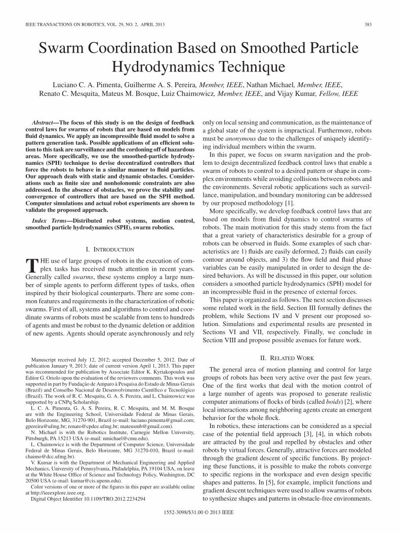
TABLE ISIMULATION PARAMETERS

A. Robustness to Localization Errors

In the two examples that are presented in this section, we usedthe parameters that are shown in Table I. The values of ξ1 , ξ2 ,and η2 are recommended values that are described in [28]. Sinceg is the gravity acceleration, its value is a standard value. Thedamping ζ was tuned to avoid intense oscillatory behavior closeto the target region. The values of γ and H were experimentallytuned by observing the system behavior during simulations. Weverified that these parameters influenced the proximity of therobots during the task execution but were not decisive in theaccomplishment of the task.

The external force gain k was determined in order to providea force component larger than those obtained from pressuregradient. This means that converging to the target has priorityover controlling density.

The most important parameters to tune are the mass mi andthe parameter h. These parameters are used in the computationof the density, and together with the reference density ρ0 , theyaffect directly the distance the robots try to keep from theirneighbors.

As the value 2h determines the size of the robot’s neighbor-hood, the smoothing length h is determined according to thehardware of the robots. If the robots receive state informationfrom their neighbors via communication, we set 2h as the com-munication radius. In the following simulations, we assumed acommunication radius of 0.1 m.

We also assumed circular small robots with radius R = 5 mm.This value corresponds to 0.1h, i.e., the communication radiusis 20 times larger than the physical radius of the robot. Thisrelation is reasonable for actual robotic platforms. Regardingrobustness to localization errors, we designed the parameter εin (31) in order to avoid collisions even if a Gaussian randomnoise with zero mean and standard deviation σN = 2 mm isadded to the estimate of the robots position. Indeed, this noiserepresents an imprecise localization system, as 3σN is largerthan the robots radii and given by

ε = 6σN .

One may interpret the aforementioned equation as a robot radiusgrowing strategy. Given the properties of a zero mean Gaussiannoise, we can assume that the estimate of a robot position willbe confined to a circle that is centered at the correct position


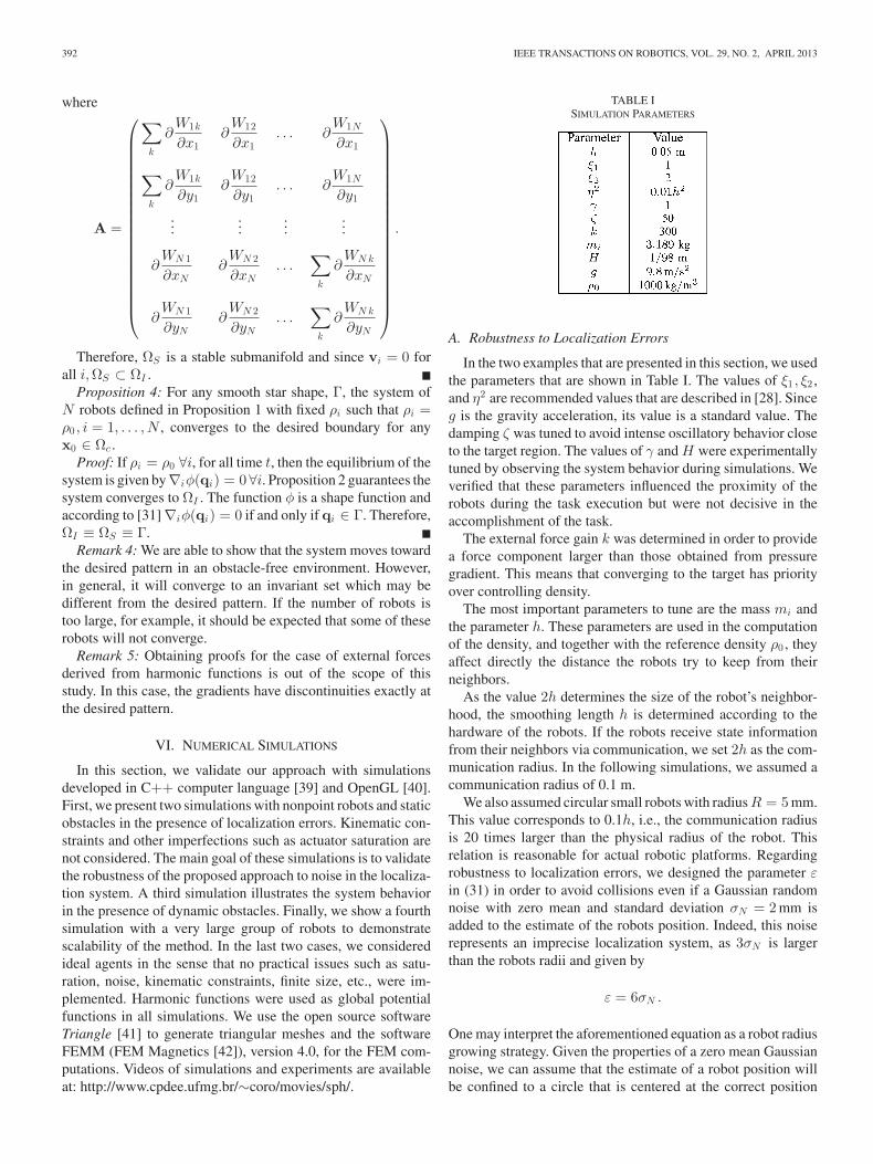
Fig. 5. Simulation with 81 point robots in a simple environment from a startingconfiguration (a) to the goal (c), with intermediate configuration (b).

TABLE IISUCCESS RATE IN THE PRESENCE OF LOCALIZATION

ERRORS—SIMPLE ENVIRONMENT

Noise Standard Deviation (σN ) Success Rate0.002 100%0.005 100%0.006 90%0.007 60%

with radius equal to 3σN . Therefore, we grow the robot size byadding ε/2 = 3σN to its actual radius.

The localization noise and robot radius were also taken intoaccount to compute the mass mi . If the distance between tworobots is smaller than 2R + ε (0.022 m, in our example), thechance of having a collision increases. Thus, we computemi so that the robots repel each other before reaching sucha distance value. We arbitrarily chose the reference densityρ0 = 1000 kg/m3 (this is the density of water) and computemi to guarantee repulsion for distances smaller than 0.5h, inthis case, 0.025 m:

mi =1000

W (0, 0.05) + W (0.5, 0.05)

where W is given by (4), resulting in a value of mass equal to3.189 kg.

1) Example 1: We first evaluated the system behavior in thepresence of localization errors in a simple environment witha single rectangular static obstacle and 81 robots. A trial ispresented in Fig. 5. Table II summarizes the obtained results fordifferent values additive Gaussian noise that is introduced intothe robot state estimates (position and velocity). We ran ten trialsfor each standard deviation σN with success that is determinedby the convergence of all robots to the target without collisionsbetween robots, walls, or obstacles.

One can note that the robots performed well even in thepresence of localization errors with a standard deviation higherthan expected, validating the robustness of our approach. Theparameters of the controller were set assuming σN = 0.002, butwe observed 100% success rate in the case of σN ≤ 0.005.

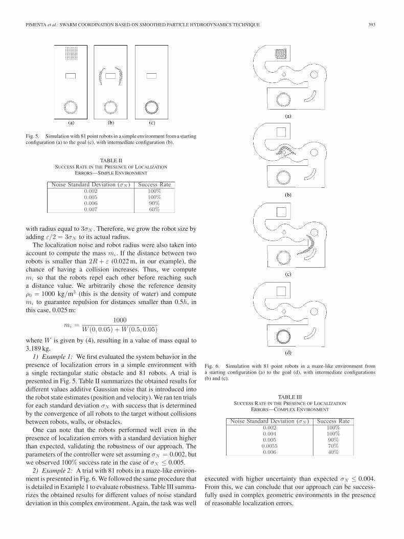
2) Example 2: A trial with 81 robots in a maze-like environ-ment is presented in Fig. 6. We followed the same procedure thatis detailed in Example 1 to evaluate robustness. Table III summa-rizes the obtained results for different values of noise standarddeviation in this complex environment. Again, the task was well

Fig. 6. Simulation with 81 point robots in a maze-like environment froma starting configuration (a) to the goal (d), with intermediate configurations(b) and (c).

TABLE IIISUCCESS RATE IN THE PRESENCE OF LOCALIZATION

ERRORS—COMPLEX ENVIRONMENT

Noise Standard Deviation (σN ) Success Rate0.002 100%0.004 100%0.005 90%0.0055 70%0.006 40%

executed with higher uncertainty than expected σN ≤ 0.004.From this, we can conclude that our approach can be success-fully used in complex geometric environments in the presenceof reasonable localization errors.


Fig. 7. One hundred ninety six robots generating a circle pattern in the pres-ence of dynamic particle obstacles.

B. Dynamic Obstacles

Fig. 7 presents different time samples of a simulation thatconsiders three dynamic particle obstacles. These obstacles arerepresented by stars (*) and are both unknown a priori andmobile. Two of these obstacles have periodic horizontal move-ment, and one of them has a periodic vertical movement. In thiscase, we used the very dense particles idea to allow the swarmto avoid obstacles (see Section V-C). We used σ = 10 to com-pute the mass of the particle obstacles. The robots are initiallydistributed in a 14 × 14 matrix.

From Fig. 7, one can conclude that the idea of consideringdynamic obstacles as very dense particles is feasible. When aparticle obstacle reaches the range of action of a swarm particle,i.e., when the distance between these two particles is smallerthan 2h, the swarm particle is subject to the influence of avirtual repulsive force and the obstacle is properly avoided. It isinteresting to mention that even in the target region, the particlesare still able to avoid the dynamic obstacles.

In this simulation, the value of the swarm particle mass waschosen to be ρ0h

2 . This mass value provides repulsion betweenagents if a robot has more than four neighbors at distancessmaller than or equal to h. Except for the mass, the other pa-rameters were those presented in Table I.

C. Very Large Groups

In this section, we show a simulation in a complex environ-ment similar to the one in Fig. 6 with a very large group. We con-sidered 1600 robots that navigate in a maze-like environment.In order to fit such a number of robots into this environment,we decreased the smoothing length to 0.02 m. This value of hallows the agents to move closer to each other. As in the lastexample, we have also set mi = ρ0h

2 , and the other parameterswere those presented in Table I. Fig. 8 shows a typical trial withthis simulation setup. All of the robots converged without colli-sions, as expected. This simulation demonstrates the scalabilityof our approach.

VII. EXPERIMENTS

In this section, we present experimental results that verify theproposed approach for finite size, nonholonomic robots. For all

Fig. 8. Simulation with 1600 point robots in a maze-like environment froma starting configuration (a) to the goal (d), with intermediate configurations (b)and (c).

experiments, the static, global vector field is computed using theFEM, which, in our case, relies on a Delaunay Triangulation-based mesh (see [35] for details).

A. First Set of Experiments

1) Experimental Setup: In [8], we presented experimen-tal results that are obtained using the experimental testbedfor multirobot experiments developed at the GRASP (Gen-eral Robotics, Automation, Sensing, and Perception) Labo-ratory at the University of Pennsylvania, Philadelphia. Thistestbed is composed of differential drive, kinematically con-trolled robots called Scarabs (see Fig. 9) and an overhead


Fig. 9. The 20 × 13.5 × 22.2 cm3 differential drive robotics platform.

tracking system that provides pose information in a global ref-erence frame.

Each Scarab is equipped with an onboard 1-GHz computer,power management system, wireless communication, and is ac-tuated by stepper motors. The tracking system consists of sevenIEEE 1394 cameras, computers, and tracking targets at the topof the robots (see Fig. 9). An extended Kalman filter (EKF) isused to fuse the information from multiple cameras. An EKFalso runs in each robot to fuse the local odometry and the over-head tracking information. This system has been successfullyused to track tens of robots simultaneously with a position errorof approximately 2 cm and an orientation error of 5◦ at 29 Hzin a 9 × 6 × 6 m3 room.

At the software level, the GRASP platform uses the open-source software that is developed by the Player/Stage/Gazebo(PSG) project [43]. Player is a network server for robot control.It provides the interfaces such that one can easily have accessto the robot’s sensors and actuators over an IP network. Thefluid-based approach was successfully implemented in the giventestbed. The algorithms were coded in C++ in the form of aPlayer driver. Further details of this infrastructure are describedin [44].

2) Results: In this set of experiments, we used a team ofseven Scarabs. The team of robots were provided with a mapof the environment which was defined by the boundaries of theexperimental area and static obstacles. A vector field that wasbased on harmonic functions was computed offline. Each robotcomputed its location in the map that is based on localizationinformation from the overhead tracking system and current ve-locity from its motor controller. This information was broadcastover the network together with the necessary SPH parameters(mass and density) to the other robots. To emulate the conceptof neighborhoods in the smaller experimental area, each robotignored messages from robots a distance greater than 2 m. Atevery update of the control algorithm, each robot computed itscurrent SPH state based on its local information and the in-formation received over the network. Additionally, each robotused virtual particles that are based on the map within a re-gion 2h′ × 2h′, with h′ = 0.3 m. During the experimentation,the algorithm was found to be more robust when multiple vir-tual particles were defined. Each virtual particle was assigned toeach cell with an obstacle in a local occupancy grid (see Fig. 4).

A vignette of one trial run of the implementation is shown inFig. 11. The team of robots started in an initial configuration [seeFig. 11(a)] and was given a circular goal formation. The control

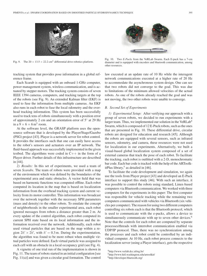
Fig. 10. Two E-Pucks from the VeRLab Swarm. Each E-puck has a 7-cmdiameter and is equipped with encoders and bluetooth communication, amongother resources.

law executed at an update rate of 10 Hz while the interagentnetwork communications executed at a higher rate of 20 Hzto accommodate the asynchronous system design. One can seethat two robots did not converge to the goal. This was dueto limitations of the minimum allowed velocities of the actualrobots. As one of the robots already reached the goal and wasnot moving, the two other robots were unable to converge.

B. Second Set of Experiments

1) Experimental Setup: After verifying our approach with agroup of seven robots, we decided to run experiments with alarger team. Thus, we implemented our solution in the VeRLab4

Swarm, which is composed of 12 E-Puck robots, such as the onesthat are presented in Fig. 10. These differential drive, circularrobots are designed for education and research [45]. Althoughthe robots are equipped with several sensors, such as infraredsensors, odometry, and camera, these resources were not usedfor localization in our experiments. Alternatively, we built avisual-based global localization system composed of a set ofexternal cameras that track the pose of each robot. To facilitatethe tracking, each robot is outfitted with a 2-D, monochromaticbar code. Each bar code is tracked with the help of the ARToolk-itPlus library,5 as detailed in [46].

To facilitate the code development and simulation, we againuse the tools from Player project [43] and developed an E-Puckinterface to support this study [46]. With such an interface, itwas possible to control the robots using standard, Linux-basedcomputers via Bluetooth communication. We worked with threecomputers for the experiments in this paper: The first computerwas responsible for vehicle tracking while the remaining twocomputers communicated with vehicles via Bluetooth (six vehi-cles per computer). The reason for using two different computerscontrolling six robots each is that the Bluetooth protocol, whichis used to communicate with the e-pucks, allows a device tosimultaneously communicate with up to seven other devices.6

Note that the controls for each robot are computed by separateprocesses/threads with interrobot communication enabled viaUDP/IP protocol. Thus, there was no synchronization amongthe processes and each robot could be controlled by an indi-vidual computer. At 10 Hz, each robot process connects to thelocalization server (using a Player interface), gets the respective

4http://www.verlab.dcc.ufmg.br/5http://www.hitl.washington.edu/artoolkit/6http://developer.bluetooth.org/


Fig. 11. Experimental Results. A team of seven robots, starting from an initialconfiguration [see Fig. 11(a)], control around an obstacle [see Figs. 11(c),(e), and (g)] to a goal circular formation [see Fig. 11(i)]. The results in theconfiguration space are also shown in Figs. 11(b), (d), (f), (h), and (j).

robot pose, and broadcasts this information along with the ve-locities from the robot encoders and the SPH parameters (massand density).

Fig. 12. Snapshots from the first experiment.

Fig. 13. Data for the experiment in Fig. 12. Path of each robot in the swarm(at left) and each robot density evolution (at right).

Fig. 14. Snapshots from the second experiment.

Fig. 15. Data for the experiment in Fig. 14. The path of each robot in theswarm (left) and the evolution of the density of individual robots (right). Noticethat the robots start behind the rectangular obstacle and move toward the circulartarget.

We performed experiments with the 12 robots in two differentworkspaces: one that is free of obstacles with a star-shaped targetand another one with a single rectangular obstacle and a circulartarget. As the robots are circular, we assume a simplified 2-Dconfiguration space (orientation is ignored) that is obtained bysimply enlarging the workspace obstacles by the robot radius.

2) Results: Fig. 12 shows four snapshots of the first experi-ment while Fig. 13 presents the robots’ paths in the correspond-ing configuration space as seen by the localization system. Notethat the swarm converges to the target and collisions are avoided.Fig. 13 also presents, at the right-hand side, the evolution of therobots’ density. As expected, this variable converges to valuesclose to the reference value of 1000 kg/m3 .

Another set of experiments was performed with a differentconfiguration space. Snapshots of a trial where all robots startbehind the obstacle is presented in Fig. 14. The robots’ pathsand densities are depicted in Fig. 15. Again, note that the swarmreached the target while avoiding collisions. The densities con-verged to values close to the reference value.


The spikes and noise present in Fig. 15 follow directly fromthe noise in the localization system (i.e., increased uncertaintyin the position estimate resulted in higher noise in the density).Note that the density [see (37)] is a nonlinear function of theposition of the robot and of its neighbors. We should mentionthat during the experiments certain regions of the workspacewere subject to worse position estimation than others due toissues in our localization system.

VIII. CONCLUSION

In this study, we have proposed a novel approach to controlswarms of robots. Our approach is scalable and does not requirethe labeling of individual robots. Therefore, all of the robots runthe same software and the success of the task execution is notdependent on specific members of the group. The approach isalso robust to the dynamic deletion and addition of new agents.

We propose to use the SPH simulation technique to createan abstract representation of the swarm as an incompressiblefluid subjected to an external force. Control of the incompress-ible fluid density provides a loose way of controlling the swarmconnectivity. We also use the FEM to compute harmonic func-tions that determine force external to the fluid. These forces aremainly responsible to drive the swarm to a desired region ofthe workspace. As obstacles may have generic geometries, theuse of the FEM allows for efficient function computation. Bymeans of a weak coupling between the FEM and the SPH, thederived controllers are decentralized in the sense that only localinformation is used by each robot of the group, including thegradient of the harmonic function at the location of the robot aswell as the position, velocity, mass, and density of the robot andits neighbors.

The proposed approach was successfully instantiated in apattern generation task. Although we presented our approachconsidering patterns as 1-D sets, it is straightforward to im-plement it in the case of patterns that are determined by othertypes of subsets of R2 such as 2-D sets, point collections, andeven disjoint sets. Techniques to accommodate actual robot fea-tures such as finite size and nonholonomic constraints (morespecifically a nonsideslipping constraint) are proposed. This isaccomplished by using feedback linearization and by adaptingthe artificial viscosity term in the SPH formulation. The vec-tor field that is computed from the designed harmonic functionhelps to avoid collisions between robots and static obstacles.However, the vector field design may be not enough to ensurethat no collisions occur. A strategy that places virtual particles atthe boundaries of the obstacles is proposed to provide collisionavoidance. By using the idea of very dense SPH particles, themethod is also able to deal with dynamic obstacles.

Computer simulations and actual robot experiments were per-formed showing the efficacy of the method. Based on the resultsof the presented simulations, we can conclude that the proposedapproach is able to deal with localization errors, dynamic obsta-cles, and swarms with more than a thousand agents. The actualexperiments were carried out using two different experimentinfrastructures: one built at the GRASP Laboratory at the Uni-versity of Pennsylvania and one at the Universidade Federal de

Minas Gerais (UFMG), Brazil. These experiments suggest thatour strategy works well for small groups of robots.

The main limitation of the method is in the number of param-eters as the success in the task execution depends on the param-eter tuning. Although our method worked well in environmentswith some narrow passages, such as in Fig. 14, issues may ariseif the parameters are not properly selected. The mass, kernelparameter h, and reference density are relevant in this case dueto their impact on interrobot spacing. The external force gaink is also relevant as it determines the vehicle bias toward thetarget and should, in principle, balance the SPH forces in thecase of narrow passages to avoid deadlocks. Nevertheless, wefound that it was not difficult to tune these variables in our sim-ulations and experiments. In Section VI-A, we detail the tuningprocedure that was used to generate our results. Although wedo not have an optimal strategy for this process, the results thatwere obtained with the presented procedure were satisfactory.

Another limitation of the method is the amount of requiredinformation. Each robot needs global localization, a completemap of the environment, and the range, bearing, and velocity ofneighboring robots. However, these requirements are consistentwith most multirobot path planning approaches. We assume thatall of this information may be provided by a different layer ofsoftware in the robotic architecture.

In principle, our method is not limited by the geometry of thepattern or of the environment as long as the number of robotsis adequate, the parameters are properly tuned, and Laplace’sequation is numerically solved with the necessary numericalprecision.

A possible direction for future work is to consider differentcooperative tasks with new fluid models. We are interested instudying how the effects of defining different values of den-sity over the environment may enable applications that requiredifferent concentrations of agents in different regions of the en-vironment. Phase transitions may also be an interesting topic toinvestigate. In the problem of object manipulation, where therobots must transport an object from one point to another, forexample, we could require that the fluid transform phase into asolid after the robots have surrounded the object and then trans-port the object by controlling the vehicles as a solid. We arealso interested in studying the impact of actuator saturation andspeed limits on the controller performance.

REFERENCES

[1] E. Sahin, “Swarm robotics: From sources of inspiration to domains ofapplication,” in Swarm Robotics (Lecture Notes in Computer ScienceSeries), E. Sahin and W. Spears, Eds. Heidelberg/Berlin: Springer-Verlag,2005, vol. 3342, pp. 10–20.

[2] C. W. Reynolds, “Flocks, herds and schools: A distributed behavioralmodel,” in Proc. Conf. Comp. Graph., Assoc. Comput. Mach., 1987,pp. 25–34.

[3] O. Khatib, “Real-time obstacle avoidance for manipulators and mobilerobots,” Intl. J. Robot. Res., vol. 5, no. 1, pp. 90–98, Mar. 1986.

[4] R. C. Arkin and T. Balch, “Aura: Principles and practice in review,” J.Exp. Theo. AI, vol. 9, no. 2–3, pp. 175–189, 1997.

[5] M. A. Hsieh, L. Chaimowicz, and V. Kumar, “Decentralized controllers forshape generation with robotic swarms,” Robotica, vol. 26, no. 5, pp. 691–701, Sep. 2008.

[6] L. Sabattini, C. Secchi, C. Fantuzzi, and D. de Macedo Possamai,“Tracking of closed-curve trajectories for multi-robot systems,” in Proc.


IEEE/RSJ Int. Conf. Intell. Robot. Syst., Taipei, Taiwan, Oct. 2010,pp. 6089–6094.

[7] L. C. A. Pimenta, M. L. Mendes, R. C. Mesquita, and G. A. S. Pereira,“Fluids in electrostatic fields: An analogy for multi-robot control,” IEEETrans. Magn., vol. 43, no. 4, pp. 1765–1768, Apr. 2007.

[8] L. C. A. Pimenta, N. Michael, R. C. Mesquita, G. A. S. Pereira, andV. Kumar, “Control of swarms based on hydrodynamic models,” in Proc.IEEE Int. Conf. Robot. Autom., Pasadena, CA, May 2008, pp. 1948–1953.

[9] A. Shaw and K. Mohseni, “A fluid dynamic based coordination of awireless sensor network of unmanned aerial vehicles: 3–D simulation andwireless communication characterization,” IEEE Sens. J., vol. 11, no. 3,pp. 722–736, Mar. 2011.

[10] D. Lipinski and K. Mohseni, “A master-slave fluid cooperative controlalgorithm for optimal trajectory planning,” in Proc. IEEE Int. Conf. Robot.Autom., Shangai, China, May 2011, pp. 3347–3351.

[11] S. Zhao, S. Ramakrishnan, and M. Kumar, “Density-based control ofmultiple robots,” in Proc. Amer. Contr. Conf., San Francisco, CA, Jun.2011, pp. 481–486.

[12] W. Spears, D. Spears, R. Heil, W. Kerr, and S. Hettiarachchi, “An overviewof physicomimetics,” Swarm Robotics (Lecture Notes in Computer Sci-ence Series), E. Sahin and W. Spears, Eds. Heidelberg/Berlin: Springer-Verlag, 2005, vol. 3342, pp. 84–97.

[13] W. Kerr, D. Spears, W. Spears, and D. Thayer, “Two formal gas modelsfor multi-agent sweeping and obstacle avoidance,” in Formal Approachesto Agent-Based Systems (Lecture Notes in Computer Science Series),M. Hinchey, J. Rash, W. Truszkowski, and C. Rouff, Eds. Heidelberg/Berlin: Springer-Verlag, 2005, vol. 3228, pp. 111–130.

[14] W. Kerr and D. Spears, “Robotic simulation of gases for a surveillancetask,” in Proc. IEEE/RSJ Int. Conf. Intell. Robot. Syst., Edmonton, AB,Canada, Aug. 2005, pp. 2905–2910.

[15] M. Shimizu, A. Ishiguro, T. Kawakatsu, Y. Masubuchi, and M. Doi, “Co-herent swarming from local interaction by exploiting molecular dynamicsand stokesian dynamics methods,” in Proc. IEEE/RSJ Int. Conf. Intell.Robot. Syst., Las Vegas, NV, May 2003, vol. 2, pp. 1614–1619.

[16] R. Narain, A. Golas, S. Curtis, and M. C. Lin, “Aggregate dynamics fordense crowd simulation,” ACM Trans. Graph., vol. 28, no. 5, pp. 122:1–122:8, Dec. 2009.

[17] M. Okada and Y. Homma, “Amenity design for congestion reductionbased on continuum model of swarm,” in Proc. Int. Conf. Mechatron.Tech., 2009, pp. 1–6.

[18] E. Sifakis, S. Marino, and J. Teran, “Globally coupled collision han-dling using volume preserving impulses,” in Proc. ACM SIGGRAPH/Eurograph. Symp. Comp. Animat., Pasadena, CA, 2008, pp. 147–153.

[19] J. R. Perkinson and B. Shafai, “A decentralized control algorithm forscalable robotic swarms based on mesh-free particle hydrodynamics,” inProc. IASTED Int. Conf. Robot. Appl., 2005, pp. 1–6.

[20] M. R. Pac, A. M. Erkmen, and I. Erkmen, “Control of robotic swarm be-haviors based on smoothed particle hydrodynamics,” in Proc. IEEE/RSJInt. Conf. Intell. Robot. Syst., San Diego, CA, Oct. 2007, pp. 4194–4200.

[21] W. J. Pisano, D. A. Lawrence, and K. Mohseni, “Concentration gradientand information energy for decentralized UAV control,” in Proc. AIAAGuid. Navigat. Contr. Conf., 2006, pp. 3283–3296.

[22] A. Howard, M. J. Mataric, and G. S. Sukhame, “Mobile sensor networkdeployment using potential fields: A distributed, scalable solution to thearea coverage problem,” in Proc. Int. Sym. Distrib. Auton. Syst., Fukuoka,Japan, Jun. 2002, pp. 299–308.

[23] M. Kloetzer and C. Belta, “Hierarchical abstractions for robotic swarms,”in Proc. IEEE Int. Conf. Robot. Autom., Orlando, FL, May 2006, pp. 952–957.

[24] C. Belta, G. A. S. Pereira, and V. Kumar, “Abstraction and control forswarms of robots,” in Robotics Research (Springer Tracts in AdvancedRobotics Series), P. Dario and R. Chatila, Eds. Heidelberg/Berlin:Springer-Verlag, 2005, vol. 15, pp. 224–233.

[25] L. B. Lucy, “A numerical approach to the testing of the fission hypothesis,”Astronom. J., vol. 82, no. 12, pp. 1013–1024, Dec. 1977.

[26] R. A. Gingold and J. J. Monaghan, “Smoothed particle hydrodynamics:Theory and application to non-spherical stars,” Month. Notic. Royal As-tronom. Soc., vol. 181, pp. 375–389, Nov. 1977.

[27] G. R. Liu and M. B. Liu, Smoothed Particle Hydrodynamics—A MeshfreeParticle Method. Singapore, World Scientific, 2003.

[28] J. J. Monaghan, “Smoothed particle hydrodynamics,” Annu. Rev. Astron.Astrophys., vol. 30, pp. 543–574, 1992.

[29] J. J. Monaghan, “Simulating free surface flow with SPH,” J. Comput.Phys., vol. 110, pp. 399–406, 1994.

[30] T. M. Roy, “Physically based fluid modeling using smoothed particlehydrodynamics,” Master’s thesis, Graduate College, Univ. Illinois, Cham-paign, IL, 1995.

[31] M. A. Hsieh and V. Kumar, “Pattern generation with multiple robots,” inProc. IEEE Int. Conf. Robot. Autom., Orlando, FL, May. 2006, pp. 2442–2447.

[32] C. I. Connolly, J. B. Burns, and R. Weiss, “Path planning using Laplace’sequation,” in Proc. IEEE Int. Conf. Robot. Autom., May 1990, pp. 2102–2106.

[33] K. P. Valavanis, T. Hebert, R. Kolluru, and N. Tsourveloudis, “Mobilerobot navigation in 2-D dynamic environments using an electrostatic po-tential field,” IEEE Trans. Syst. Man Cybern. A, Syst. Humans, vol. 30,no. 2, pp. 187–196, Mar. 2000.

[34] L. C. A. Pimenta, A. R. Fonseca, G. A. S. Pereira, R. C. Mesquita,E. J. Silva, W. M. Caminhas, and M. F. M. Campos, “On computingcomplex navigation functions,” in Proc. IEEE Int. Conf. Robot. Autom.,Barcelona, Spain, May 2005, pp. 3463–3468.

[35] L. C. A. Pimenta, A. R. Fonseca, G. A. S. Pereira, R. C. Mesquita,E. J. Silva, W. M. Caminhas, and M. F. M. Campos, “Robot navigationbased on electrostatic field computation,” IEEE Trans. Magn., vol. 42,no. 4, pp. 1459–1462, Apr. 2006.

[36] E. Rimon and D. E. Koditschek, “Exact robot navigation using artificialpotential functions,” IEEE Trans. Robot. Autom., vol. 8, no. 5, pp. 501–518, Oct. 1992.

[37] C. Belta, G. A. S. Pereira, and V. Kumar, “Control of a team of car-likerobots using abstractions,” in Proc. IEEE Conf. Decis. Contr., Maui, HI,Dec. 2003, pp. 1520–1525.

[38] J. P. Desai, J. Ostrowski, and V. Kumar, “Controlling formations of mul-tiple mobile robots,” in Proc. IEEE Int. Conf. Robot. Autom., Leuven,Belgium, May 1998, pp. 2864–2869.

[39] B. Stroustrup, The C++ Programming Language, Third ed. Reading,MA: Addison-Wesley, 2000.

[40] D. Shreiner, M. Woo, J. Neider, and T. Davis, OpenGL(R) Program-ming Guide: The Official Guide to Learning OpenGL(R), Ver. 2, Fifth ed.Reading, MA: Addison-Wesley, 2005.

[41] J. Shewchuk, “Triangle: Engineering a 2D quality mesh generator anddelaunay triangulator,” in Applied Computational Geometry TowardsGeometric Engineering (Lecture Notes Comput. Sci.), M. Lin and D.Manocha, Eds., Heidelberg/Berlin, Germany: Springer-Verlag, 1996,vol. 1148, pp. 203–222.

[42] D. Meeker, Finite Element Method Magnetics—User’s Manual, May2004, ver. 4.0.

[43] B. Gerkey, R. T. Vaughan, and A. Howard, “The player/stage project:Tools for multi-robot and distributed sensor systems,” in Proc. Int. Conf.Adv. Robot., Coimbra, Portugal, Jun. 2003, pp. 317–323.

[44] N. Michael, J. Fink, and V. Kumar, “Experimental testbed for large multi-robot teams: Verification and validation,” IEEE Robot. Autom. Mag.,vol. 15, no. 1, pp. 53–61, Mar. 2008.

[45] F. Mondada, M. Bonani, X. Raemy, J. Pugh, C. Cianci, A. Klaptocz,S. Magnenat, J.-C. Zufferey, D. Floreano, and A. Martinoli, “The e-puck,a robot designed for education in engineering,” in Proc. Conf. Auton.Robot. Syst. Competit., Castelo Branco, Portugal, May 2009, pp. 59–65.

[46] R. F. Garcia and L. Chaimowicz, “An experimental infrastructure forswarms of robots,” in Proc. Brazil. Symp. Intell. Autom., Brasilia, Brazil,Sep. 2009, pp. 1–6, (in Portuguese).

Luciano C. A. Pimenta received the B.S., M.Sc.,and Ph.D. degrees in electrical engineering fromthe Universidade Federal de Minas Gerais (UFMG),Belo Horizonte, Brazil, in 2003, 2005, and 2009,respectively.

He is currently an Assistant Professor with the De-partment of Electronic Engineering at UFMG. Hisresearch interests include robotics, multirobot sys-tems, and control theory. From April 2007 to June2008, he was a visiting Ph.D. student with the Gen-eral Robotics, Automation, Sensing, and Perception

Laboratory, University of Pennsylvania, Philadelphia.


Guilherme A. S. Pereira (M’12) received the B.S.and M.S. degrees in electrical engineering and thePh.D. degree in computer science from the FederalUniversity of Minas Gerais (UFMG), Belo Horizonte,Brazil, in 1998, 2000, and 2003, respectively.

He was, from November 2000 to May 2003, a Vis-iting Scientist with the General Robotics, Automa-tion, Sensing, and Perception Laboratory, Universityof Pennsylvania, Philadelphia. Since July 2004, hehas been an Assistant Professor with the Departmentof Electrical Engineering, Federal University of Mi-

nas Gerais, where he is the Director of the Computer Systems and Robotics Lab-oratory, which is one of the laboratories that compose the Group for Researchand Development of Autonomous Vehicles, UFMG. His research interests in-clude cooperative robotics, robot navigation, autonomous vehicles development,computer vision, and distributed sensing.

Dr. Pereira is a Member of Sociedade Brasileira de Automatica. He receivedthe Gold Medal Award from the Engineering School of UFMG for garneringfirst place among the electrical engineering students in 1998.

Nathan Michael (M’09) is an Assistant ResearchProfessor in the Robotics Institute at CarnegieMellon University. Prior to this appointment, hewas a Research Assistant Professor in the Depart-ment of Mechanical Engineering at the University ofPennsylvania. He received a Ph.D. from the Depart-ment of Mechanical Engineering at the University ofPennsylvania in 2008 and transitioned into a positionin the Research Faculty in 2010. His research inter-ests include the topics of estimation and control forground and aerial robots with extensions to multi-

robot systems.

Renato C. Mesquita was born in Belo Horizonte,Brazil, in 1959. He received the B.S. and M.S. de-grees in electrical engineering from the Federal Uni-versity of Minas Gerais, Belo Horizonte, Brazil, in1982 and 1986, respectively, and the Dr. degree inelectrical engineering from the Federal University ofSanta Catarina, Florianopolis, Brazil, in 1990.

Since 1983, he has been with the Department ofElectrical Engineering, Federal University of MinasGerais, where he is currently an Associate Professor.His main research interest is in the area of electro-

magnetic field computation. He has authored or coauthored more than 150journal and conference papers in this area.

Mateus M. Bosque received the B.S. degree in con-trol and automation engineering from the FederalUniversity of Minas Gerais, Belo Horizonte, Brazil,in 2010.

He is currently with Federal University of MinasGerais. He has experience in robotics and computerprogramming. His current research interests includeinformation technology and the development of com-puter systems to process financial data.

Luiz Chaimowicz (M’12) received the Ph.D. degreein computer science from the Universidade Federalde Minas Gerais (UFMG), Belo Horizonte, Brazil, in2002.

From 2003 to 2004, he held a Postdoctoral Re-search Appointment with the General Robotics, Au-tomation, Sensing, and Perception Laboratory, Uni-versity of Pennsylvania, Philadelphia. He is currentlyan Associated Professor with the Department of Com-puter Science, UFMG, where he co-directs UFMGsComputer Vision and Robotics Laboratory, which

conducts research on several aspects of computer vision and mobile robotics.His recent research focuses on the coordination and control of large groupsof robots and the development of collision-free navigation strategies for thesegroups.

Vijay Kumar (F’06) is the UPS Foundation Profes-sor in the School of Engineering and Applied Scienceat the University of Pennsylvania, and on sabbaticalleave at White House Office of Science and Technol-ogy Policy where he serves as the assistant directorfor robotics and cyber physical systems. He receivedhis Bachelors of Technology from the Indian Instituteof Technology, Kanpur and his Ph.D. from The OhioState University in 1987. He has been on the Facultyin the Department of Mechanical Engineering andApplied Mechanics with a secondary appointment in

the Department of Computer and Information Science at the University of Penn-sylvania since 1987.

He served as the Deputy Dean for Research in the School of Engineeringand Applied Science from 2000-2004. He directed the GRASP Laboratory, amultidisciplinary robotics and perception laboratory, from 1998–2004. He wasthe Chairman of the Department of Mechanical Engineering and Applied Me-chanics from 2005-2008. He then served as the Deputy Dean for Education inthe School of Engineering and Applied Science from 2008- 2012.

Dr. Kumar is a Fellow of the American Society of Mechanical Engineers(ASME) and the Institute of Electrical and Electronic Engineers. He has servedon the editorial boards of the IEEE TRANSACTIONS ON ROBOTICS AND AU-TOMATION, IEEE TRANSACTIONS ON AUTOMATION SCIENCE AND ENGINEER-ING, ASME Journal of Mechanical Design, the ASME Journal of Mechanismsand Robotics and the Springer Tract in Advanced Robotics (STAR). He is therecipient of the 1991 National Science Foundation Presidential Young Investi-gator award, the 1996 Lindback Award for Distinguished Teaching (Universityof Pennsylvania), the 1997 Freudenstein Award for significant accomplishmentsin mechanisms and robotics, the 2012 ASME Mechanisms and Robotics Award,the 2012 IEEE Robotics and Automation Society Distinguished Service Awardand a 2012 World Technology Network Award. He has won best paper awards atDARS 2002, ICRA 2004, ICRA 2011, and RSS 2011 and has advised doctoralstudents who have won Best Student Paper Awards at ICRA 2008, RSS 2009,and DARS 2010. He is also a Distinguished Lecturer in the IEEE Robotics andAutomation Society and an elected member of the Robotics and AutomationSociety Administrative Committee (2007-2012). His research interests are inrobotics, specifically multi-robot systems, and micro aerial vehicles.

Documents

IEEE TRANSACTIONS ON ROBOTICS, VOL. 29, NO. 2, APRIL …gpereira/papers/tro2013.pdf · Swarm Coordination Based on Smoothed Particle Hydrodynamics Technique Luciano C. A. Pimenta,