Embed Size (px)
Citation preview
IEEE TRANSACTIONS ON SIGNAL PROCESSING. VOL. 62, NO. 24, PP. 6596–6611, DEC.15, 2014 (PREPRINT) 1
Transient Artifact Reduction Algorithm (TARA)Based on Sparse Optimization
Ivan W. Selesnick, Harry L. Graber, Yin Ding, Tong Zhang, Randall L. Barbour
Abstract—This paper addresses the suppression of transientartifacts in signals, e.g., biomedical time series. To that end,we distinguish two types of artifact signals. We define ‘Type1’ artifacts as spikes and sharp, brief waves that adhere to abaseline value of zero. We define ‘Type 2’ artifacts as comprisingapproximate step discontinuities. We model a Type 1 artifact asbeing sparse and having a sparse time-derivative, and a Type2 artifact as having a sparse time-derivative. We model theobserved time series as the sum of a low-pass signal (e.g., abackground trend), an artifact signal of each type, and a whiteGaussian stochastic process. To jointly estimate the componentsof the signal model, we formulate a sparse optimization problemand develop a rapidly converging, computationally efficientiterative algorithm denoted TARA (‘transient artifact reductionalgorithm’). The effectiveness of the approach is illustrated usingnear infrared spectroscopic time-series data.
I. INTRODUCTION
This paper addresses the suppression of artifacts in mea-sured signals, where the artifacts are of unknown shape but areknown to be transient in form. We are motivated in particularby the problem of attenuating artifacts arising in biomedicaltime series, such as those acquired using near infrared spectro-scopic (NIRS) imaging devices [3]. Our approach is based ona signal model intended to capture the primary characteristicsof the artifacts, and on the subsequent formulation of anoptimization problem. We model the measured discrete-timeseries, y(n), as
y(n) = f(n) + x1(n) + x2(n) + w(n) n ∈ Z, (1)
where f is a low-pass signal, xi are two distinct types ofartifact signals, and w is white Gaussian noise. Specifically,f is low-pass in the sense that when f is used as the inputto an appropriately chosen high-pass filter, denoted by H, theoutput is approximately the all-zero signal; i.e., Hf ≈ 0.
The ‘Type 1’ artifact signal, x1, is intended to model spikesand sharp, brief waves, while the ‘Type 2’ artifact signal,x2, is intended to model additive step discontinuities. Forthe purpose of flexibility and generality, we avoid defining
Selesnick, Ding, and Zhang are with the Dept. of Electrical and ComputerEngineering, Polytechnic School of Engineering, New York University, 6Metrotech Center, Brooklyn, NY 11201. Graber and Barbour are with theDept. of Pathology, SUNY Downstate Medical Center, Brooklyn, NY 11203.Email: [email protected], [email protected].
MATLAB software is available at http://eeweb.poly.edu/iselesni/TARA/This research was supported by the NSF under Grant No. CCF-1018020,
the NIH under Grant Nos. R42NS050007, R44NS049734, and R21NS067278,and by DARPA project N66001-10-C-2008.
Copyright (c) 2014 IEEE. Personal use of this material is permitted.However, permission to use this material for any other purposes must beobtained from the IEEE by sending a request to [email protected].
the artifact signals in terms of precise rules or templates.Instead, we use the notion of sparsity to define them in aless regimented way that facilitates the formulation of anoptimization-based approach:
1) We define the ‘Type 1’ artifact signal, x1, as beingsparse and having a sparse derivative (actually, a discrete-timeapproximation of the derivative, here and subsequently).
2) We define the ‘Type 2’ artifact signal, x2, as having asparse derivative. This type of artifact signal is composed ofstep discontinuities or approximate step discontinuities.
After the artifacts, xi, are estimated, they are subtractedfrom the raw data to obtain a corrected time series.
To handle both types of artifacts simultaneously, in thiswork we develop an algorithm, denoted ‘Transient ArtifactReduction Algorithm’ (TARA). Complex artifacts often com-prise both types; hence TARA performs joint optimizationto maximize the effectiveness of the model to better reducesuch artifacts. We devise TARA to have high computationalefficiency and low memory requirements by constraining allmatrices to be banded,1 which allows us to leverage fastsolvers for banded systems [29, Sect 2.4]. Additionally, TARAdoes not require the user to specify auxiliary algorithmicparameters.
In addition to suppressing artifacts according to the model(1), we also consider the simplified model
y(n) = f(n) + x1(n) + w(n), n ∈ Z, (2)
which contains artifacts of Type 1 only. We considered model(2) in previous work [34], where we used it to formulate whatwe called the ‘LPF/CSD’ problem. In this paper we present animproved algorithm for the LPF/CSD problem and provide anapproach for setting the parameters. The new algorithm servesas the basis for the development of TARA, which suppressesartifacts according to model (1).
Although the suppression of Type 1 and Type 2 artifactswas addressed in our previous work [34], it was assumed thatthe measured time series is affected by the presence of eitherType 1 or Type 2 artifacts, but not both. Two algorithms, onefor each artifact type, are described in [34]. The respectivealgorithms were illustrated on time series acquired using aNIRS system [23], which frequently have artifacts of bothtypes [15]. The algorithms were compared with the algorithmused by the NAP software application for NIRS artifactsuppression [15].
1A matrix is banded if its non-zero elements lie only on its main diagonaland a few adjacent upper and lower diagonals.

2 IEEE TRANSACTIONS ON SIGNAL PROCESSING. VOL. 62, NO. 24, PP. 6596–6611, DEC.15, 2014 (PREPRINT)
A. Related Work
Several approaches have been developed for the suppressionof artifacts in biomedical time series [2], [9], [15], [20],[21], [25], [31], [37], [38]. Some methods, such as thosebased on independent component analysis (ICA) or adaptivefiltering, require the availability of multiple channels or refer-ence signals. However, if artifacts differ substantially amongchannels or if multiple channels are unavailable, then single-channel methods are needed [9], [21], [24]. Several methodsfor detecting and/or correcting motion artifacts in NIRS timeseries have been compared [9], [21], [24], [31], [32], leading tothe conclusion that wavelet-based methods are more effectivethan other methods, especially for single-channel processing.Wavelets have also been shown effective for reducing ocularartifacts in EEG [2], [22]. Hence, we compare the sparseoptimization and wavelet approaches below.
We remark that models (1) and (2) are prompted by theapproach of morphological component analysis (MCA), inwhich all signal components are modeled as sparse withrespect to distinct transforms [35]. However, the presence ofthe low-pass non-sparse component, f , which differs fromMCA, makes models (1) and (2) more realistic for biomedicaltime-series analysis. Moreover, modeling the low-pass com-ponent enhances the prospective sparsity of the remainingcomponents, on which sparse optimization and MCA rely.
Rather than developing optimization schemes for generallinear inverse problems, this work emphasizes algorithmsthat exploit the banded structure of one-dimensional lineartime-invariant (LTI) operators to achieve high computationalefficiency and fast convergence while avoiding additional al-gorithm parameters (e.g., step-size parameters), for the specificproblems considered here. Yet, we note that general optimiza-tion algorithms, such as those based on proximity operators[8], [10], [12], [13], [28], [30], allow for consideration of non-smooth compound regularization problems more general thanthose considered here. Relevant surveys are also given in [4],[36].
B. Notation
Vectors and matrices are represented by lower- and upper-case bold (e.g., x and H), respectively. The n-th component ofa vector x is denoted [x]n. Finite-length discrete-time signalsare represented as vectors in RN . The notation x ∈ [a, b]means a 6 x 6 b.
II. TYPE 1 ARTIFACTS (THE LPF/CSD PROBLEM)
In this section, we consider model (2), which containsartifacts of Type 1 only. The derivation of TARA in Sec. III formodel (1) builds on the algorithm developed here. In previouswork [34], an iterative algorithm based on the ‘alternatingdirection method of multipliers’ (ADMM) was derived for the‘LPF/CSD’ problem. Here, we revisit the problem and presentseveral improvements in comparison with [34].
1) A faster algorithm. In this work, we derive an algorithmbased on majorization-minimization (MM). The new algorithmconverges in fewer iterations in practice than the previousalgorithm based on ADMM.
2) Fewer algorithm parameters. The algorithm of [34]required the user to specify a positive scalar, µ, analogousto a step-size parameter. A poor choice of µ leads to slowconvergence. The new MM algorithm does not require anyparameters beyond those in the objective function.
3) A method to set regularization parameters, λ0 and λ1,based on the noise variance (which we assume is known).
4) A more general problem formulation. In this work, weallow the penalty functions to be non-convex, whereas [34]considered convex penalty functions only. With convex penaltyfunctions, the amplitudes of artifacts tend to be underestimated(the estimates are biased toward zero).
5) A method to set non-convexity parameters. In the casewhere non-convex penalty functions are utilized, we presenta method to set the non-convexity parameters. The previouswork considered only convex penalty functions.
A. Problem formulationWe address the problem in the discrete-time setting. Signals
are represented as vectors in RN . We write model (2) as
y = f + x + w, y, x, w ∈ RN (3)
where the signal x is modeled as sparse and having a sparsederivative. The derivative is approximated using the discrete-time first-order difference operator, D, defined by [Dx]n =[x]n+1 − [x]n. The matrix D has the form
D =
−1 1
−1 1. . . . . .
−1 1
. (4)
In order to estimate x from y, we propose to solve theoptimization problem
x = argminx
{F (x) =
1
2‖H(y − x)‖22
+ λ0∑n
φ0([x]n) + λ1∑n
φ1([Dx]n)}, (5)
where λi > 0 are the regularization parameters. The low-passsignal is then estimated as
f = L(y − x) = y − x−H(y − x), (6)
where L denotes the low-pass filter defined as L = I−H. Thepenalty functions, φi : R→ R, are chosen to promote sparsity.We refer to (5) as the LPF/CSD (low-pass-filtering/compound-sparse-denoising) problem [34].
When φi is the absolute-value function, φi(x) = |x|, fori = 1, 2, then problem (5) is the same as that consideredin [34]. When, in addition, H is the identity operator, (5) isthe same as the ‘fused lasso signal approximator’ in Ref. [17].
The high-pass filter, H, is taken to be a zero-phase recursivediscrete-time filter that we write as
H = BA−1, (7)
where A and B are banded Toeplitz matrices, as describedin Sec. VI of [34]. We further suppose that B admits thefactorization
B = B1D, (8)
3
where B1 is banded and D is the above-noted first-order dif-ference matrix. (See [34] for derivations of the factorizations in(7) and (8).) The fact that A and B are banded is important forthe computational efficiency of the algorithm to be developed.We also assume that A, B1, and D commute. As LTI filters,these operators are commutative for infinite-length discrete-time signals defined on Z. For finite-length signals, withwhich we deal in practice, the operators are approximatelycommutative, with the error being confined to the start and endof the signal, with a temporal extent that depends on the time-constant of the filter. We note that H was expressed as A−1Bin our earlier work [34]. Here we express H as BA−1, whichthe commutativity property permits, because the derivation ofthe computationally efficient MM algorithm in Sec. II-B relieson this ordering. We assume in this work that the signals ofinterest are sufficiently long that start and end transients arenot problematic, in which case the commutativity assumptionis justified.
The regularization parameters, λ0 and λ1, control the rela-tive weight between the penalty terms. Their values should alsobe set according to the noise variance: higher noise calls forhigher λi. As noted in [34], the regularization in problem (5) isan example of compound regularization [1], [6], wherein twoor more regularizers are used to promote distinct properties ofthe signal to be recovered.
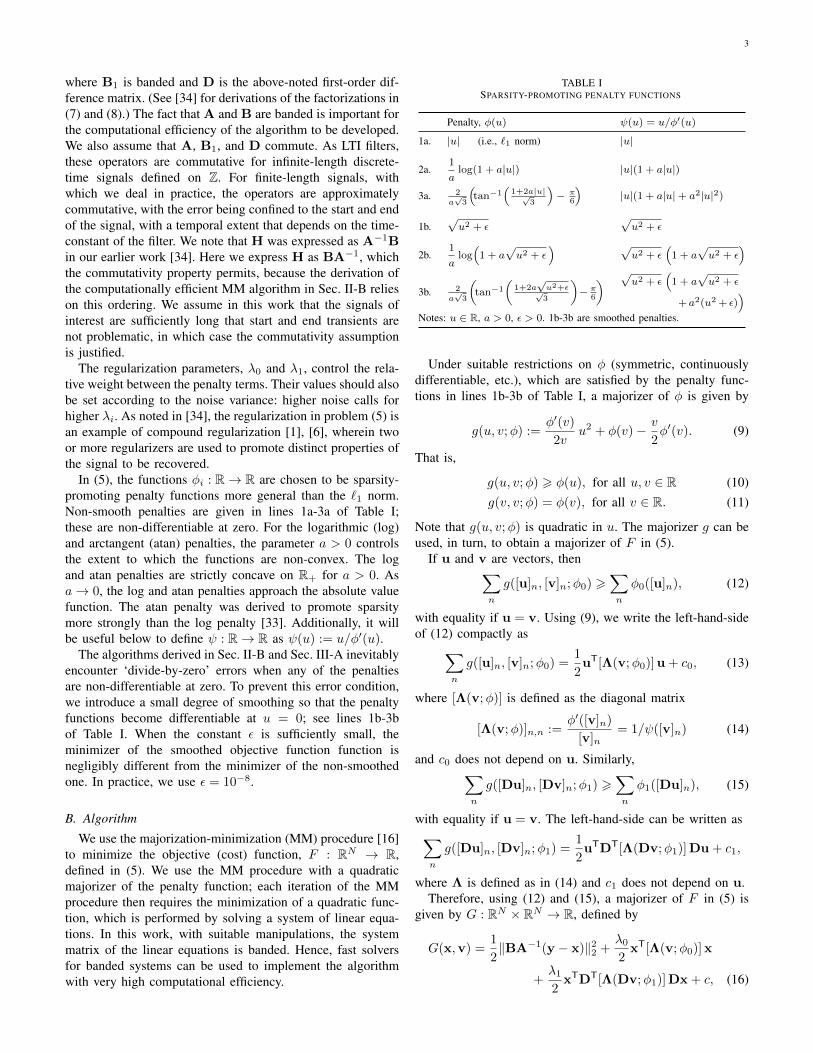
In (5), the functions φi : R→ R are chosen to be sparsity-promoting penalty functions more general than the `1 norm.Non-smooth penalties are given in lines 1a-3a of Table I;these are non-differentiable at zero. For the logarithmic (log)and arctangent (atan) penalties, the parameter a > 0 controlsthe extent to which the functions are non-convex. The logand atan penalties are strictly concave on R+ for a > 0. Asa→ 0, the log and atan penalties approach the absolute valuefunction. The atan penalty was derived to promote sparsitymore strongly than the log penalty [33]. Additionally, it willbe useful below to define ψ : R→ R as ψ(u) := u/φ′(u).
The algorithms derived in Sec. II-B and Sec. III-A inevitablyencounter ‘divide-by-zero’ errors when any of the penaltiesare non-differentiable at zero. To prevent this error condition,we introduce a small degree of smoothing so that the penaltyfunctions become differentiable at u = 0; see lines 1b-3bof Table I. When the constant ε is sufficiently small, theminimizer of the smoothed objective function function isnegligibly different from the minimizer of the non-smoothedone. In practice, we use ε = 10−8.
B. Algorithm
We use the majorization-minimization (MM) procedure [16]to minimize the objective (cost) function, F : RN → R,defined in (5). We use the MM procedure with a quadraticmajorizer of the penalty function; each iteration of the MMprocedure then requires the minimization of a quadratic func-tion, which is performed by solving a system of linear equa-tions. In this work, with suitable manipulations, the systemmatrix of the linear equations is banded. Hence, fast solversfor banded systems can be used to implement the algorithmwith very high computational efficiency.
TABLE ISPARSITY-PROMOTING PENALTY FUNCTIONS
Penalty, φ(u) ψ(u) = u/φ′(u)
1a. |u| (i.e., `1 norm) |u|
2a.1
alog(1 + a|u|) |u|(1 + a|u|)
3a. 2a√3
(tan−1
(1+2a|u|√
3
)− π
6
)|u|(1 + a|u|+ a2|u|2)
1b.√u2 + ε
√u2 + ε
2b.1
alog(
1 + a√u2 + ε
) √u2 + ε
(1 + a
√u2 + ε
)3b. 2
a√3
(tan−1
(1+2a√u2+ε√3
)− π
6
) √u2 + ε
(1 + a
√u2 + ε
+a2(u2 + ε))
Notes: u ∈ R, a > 0, ε > 0. 1b-3b are smoothed penalties.
Under suitable restrictions on φ (symmetric, continuouslydifferentiable, etc.), which are satisfied by the penalty func-tions in lines 1b-3b of Table I, a majorizer of φ is given by
g(u, v;φ) :=φ′(v)
2vu2 + φ(v)− v
2φ′(v). (9)
That is,
g(u, v;φ) > φ(u), for all u, v ∈ R (10)g(v, v;φ) = φ(v), for all v ∈ R. (11)
Note that g(u, v;φ) is quadratic in u. The majorizer g can beused, in turn, to obtain a majorizer of F in (5).
If u and v are vectors, then∑n
g([u]n, [v]n;φ0) >∑n
φ0([u]n), (12)
with equality if u = v. Using (9), we write the left-hand-sideof (12) compactly as∑
n
g([u]n, [v]n;φ0) =1
2uT[Λ(v;φ0)]u + c0, (13)
where [Λ(v;φ)] is defined as the diagonal matrix
[Λ(v;φ)]n,n :=φ′([v]n)
[v]n= 1/ψ([v]n) (14)
and c0 does not depend on u. Similarly,∑n
g([Du]n, [Dv]n;φ1) >∑n
φ1([Du]n), (15)
with equality if u = v. The left-hand-side can be written as∑n
g([Du]n, [Dv]n;φ1) =1
2uTDT[Λ(Dv;φ1)]Du + c1,
where Λ is defined as in (14) and c1 does not depend on u.Therefore, using (12) and (15), a majorizer of F in (5) is
given by G : RN × RN → R, defined by
G(x,v) =1
2‖BA−1(y − x)‖22 +
λ02
xT[Λ(v;φ0)]x
+λ12
xTDT[Λ(Dv;φ1)]Dx + c, (16)
4 IEEE TRANSACTIONS ON SIGNAL PROCESSING. VOL. 62, NO. 24, PP. 6596–6611, DEC.15, 2014 (PREPRINT)
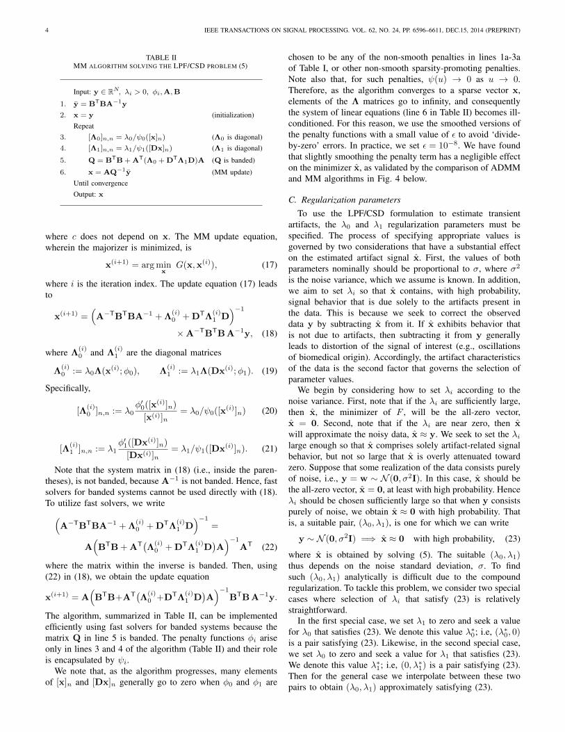
TABLE IIMM ALGORITHM SOLVING THE LPF/CSD PROBLEM (5)
Input: y ∈ RN, λi > 0, φi,A,B
1. y = BTBA−1y
2. x = y (initialization)Repeat
3. [Λ0]n,n = λ0/ψ0([x]n) (Λ0 is diagonal)4. [Λ1]n,n = λ1/ψ1([Dx]n) (Λ1 is diagonal)
5. Q = BTB + AT(Λ0 + DTΛ1D)A (Q is banded)
6. x = AQ−1y (MM update)Until convergenceOutput: x
where c does not depend on x. The MM update equation,wherein the majorizer is minimized, is
x(i+1) = argminx
G(x,x(i)), (17)
where i is the iteration index. The update equation (17) leadsto
x(i+1) =(A−TBTBA−1 + Λ
(i)0 + DTΛ
(i)1 D
)−1×A−TBTB A−1y, (18)
where Λ(i)0 and Λ
(i)1 are the diagonal matrices
Λ(i)0 := λ0Λ(x(i);φ0), Λ
(i)1 := λ1Λ(Dx(i);φ1). (19)
Specifically,
[Λ(i)0 ]n,n := λ0
φ′0([x(i)]n)
[x(i)]n= λ0/ψ0([x
(i)]n) (20)
[Λ(i)1 ]n,n := λ1
φ′1([Dx(i)]n)
[Dx(i)]n= λ1/ψ1([Dx(i)]n). (21)
Note that the system matrix in (18) (i.e., inside the paren-theses), is not banded, because A−1 is not banded. Hence, fastsolvers for banded systems cannot be used directly with (18).To utilize fast solvers, we write(
A−TBTBA−1 + Λ(i)0 + DTΛ
(i)1 D
)−1=
A(BTB + AT
(Λ
(i)0 + DTΛ
(i)1 D
)A)−1
AT (22)
where the matrix within the inverse is banded. Then, using(22) in (18), we obtain the update equation
x(i+1) = A(BTB+AT
(Λ
(i)0 +DTΛ
(i)1 D
)A)−1
BTB A−1y.
The algorithm, summarized in Table II, can be implementedefficiently using fast solvers for banded systems because thematrix Q in line 5 is banded. The penalty functions φi ariseonly in lines 3 and 4 of the algorithm (Table II) and their roleis encapsulated by ψi.
We note that, as the algorithm progresses, many elementsof [x]n and [Dx]n generally go to zero when φ0 and φ1 are
chosen to be any of the non-smooth penalties in lines 1a-3aof Table I, or other non-smooth sparsity-promoting penalties.Note also that, for such penalties, ψ(u) → 0 as u → 0.Therefore, as the algorithm converges to a sparse vector x,elements of the Λ matrices go to infinity, and consequentlythe system of linear equations (line 6 in Table II) becomes ill-conditioned. For this reason, we use the smoothed versions ofthe penalty functions with a small value of ε to avoid ‘divide-by-zero’ errors. In practice, we set ε = 10−8. We have foundthat slightly smoothing the penalty term has a negligible effecton the minimizer x, as validated by the comparison of ADMMand MM algorithms in Fig. 4 below.
C. Regularization parametersTo use the LPF/CSD formulation to estimate transient
artifacts, the λ0 and λ1 regularization parameters must bespecified. The process of specifying appropriate values isgoverned by two considerations that have a substantial effecton the estimated artifact signal x. First, the values of bothparameters nominally should be proportional to σ, where σ2
is the noise variance, which we assume is known. In addition,we aim to set λi so that x contains, with high probability,signal behavior that is due solely to the artifacts present inthe data. This is because we seek to correct the observeddata y by subtracting x from it. If x exhibits behavior thatis not due to artifacts, then subtracting it from y generallyleads to distortion of the signal of interest (e.g., oscillationsof biomedical origin). Accordingly, the artifact characteristicsof the data is the second factor that governs the selection ofparameter values.
We begin by considering how to set λi according to thenoise variance. First, note that if the λi are sufficiently large,then x, the minimizer of F , will be the all-zero vector,x = 0. Second, note that if the λi are near zero, then xwill approximate the noisy data, x ≈ y. We seek to set the λilarge enough so that x comprises solely artifact-related signalbehavior, but not so large that x is overly attenuated towardzero. Suppose that some realization of the data consists purelyof noise, i.e., y = w ∼ N (0, σ2I). In this case, x should bethe all-zero vector, x = 0, at least with high probability. Henceλi should be chosen sufficiently large so that when y consistspurely of noise, we obtain x ≈ 0 with high probability. Thatis, a suitable pair, (λ0, λ1), is one for which we can write
y ∼ N (0, σ2I) =⇒ x ≈ 0 with high probability, (23)
where x is obtained by solving (5). The suitable (λ0, λ1)thus depends on the noise standard deviation, σ. To findsuch (λ0, λ1) analytically is difficult due to the compoundregularization. To tackle this problem, we consider two specialcases where selection of λi that satisfy (23) is relativelystraightforward.
In the first special case, we set λ1 to zero and seek a valuefor λ0 that satisfies (23). We denote this value λ∗0; i.e, (λ∗0, 0)is a pair satisfying (23). Likewise, in the second special case,we set λ0 to zero and seek a value for λ1 that satisfies (23).We denote this value λ∗1; i.e, (0, λ∗1) is a pair satisfying (23).Then for the general case we interpolate between these twopairs to obtain (λ0, λ1) approximately satisfying (23).
5
In order to find λ∗0 and λ∗1, we work with two special casesof (5). We define the objective function, F0 : RN → R, as
F0(x) =1
2‖H(y − x)‖22 + λ0
∑n
φ0([x]n) (24)
and the objective function, F1 : RN → R, as
F1(x) =1
2‖H(y − x)‖22 + λ1
∑n
φ1([Dx]n). (25)
The functions F0 and F1 correspond to λ1 = 0 and λ0 = 0 in(5), respectively. Unlike F , the Fi do not involve compoundregularization, which simplifies the analysis necessary to setλi. We denote the minimizers of F0 and F1 as:
xoptF0
= argminx
F0(x), xoptF1
= argminx
F1(x). (26)
To find λ∗0 such that (λ∗0, 0) satisfies (23), we equivalentlyfind λ∗0 such that
y ∼ N (0, σ2I) =⇒ xoptF0≈ 0 with high probability. (27)
That is, we seek to set λ0 in (24) so that xoptF0
is relatively noise-free with high probability. The value for λ∗0 accomplishing thisis derived using optimality conditions from convex analysis.This general approach has been described by Fuchs [18] forthe purpose of setting the false alarm rate in a target detectionapplication. To find λ∗1 such that (0, λ∗1) satisfies (23), we willproceed in a similar manner; however, the presence of D inthe penalty of F needs to be taken into account.Obtaining λ∗0. We assume here that φ0 is one of the non-smooth penalty functions in Table I (lines 1a–3a). We will usea result from the theory of convex functions [5]: if a functionf : RN → R is convex, then x is a minimizer of f if and onlyif 0 ∈ ∂f(x), where ∂f is the subgradient of f .
As shown in [33], if φ0 is chosen such that F0 in (24) isconvex, then x minimizes F0 if and only if, for all n,
[HTH(y − x)]n
{= λ0 φ
′0([x]n), [x]n 6= 0
∈ [−λ0, λ0], [x]n = 0.(28)
When x = xoptF0
is the all-zero vector, we have
xoptF0
= 0 =⇒ [HTHy]n ∈ [−λ0, λ0], ∀n, (29)
and the right-hand-side of (27) can be written as [HTHy]n ∈[−λ∗0, λ∗0], ∀n with high probability. Hence, λ∗0 should bechosen so that
λ∗0 > |[HTHy]n|, ∀n with high probability, (30)
where y ∼ N (0, σ2I). Note that HTH represents an LTIsystem. Then HTHy is a stationary stochastic process and[HTHy]n ∼ N (0, σ2
0), where σ0 is given by
σ0 := std([HTHy]n) = ‖p0‖2 σ
and p0 is the impulse response of the LTI filter HTH. That is,p0 = h ∗ hr, where h represents the impulse response of theLTI filter H := BA−1, and hr is the time-reversed versionof h (i.e., hr(−n) = h(n)).
So, (30) can be expressed as
λ∗0 > |v|, ∀n with high probability, where v ∼ N (0, σ20).
A nominal value of λ∗0 is given by the ‘three-sigma’ rule,
λ∗0 = 3σ0 = 3 ‖p0‖2 σ. (31)
Using the λ∗0 value given by (31), (30) is satisfied with aprobability above 99%.Obtaining λ∗1. From (7) and (8), note that H = B1DA−1.Using commutativity, we have H = B1A
−1D. Henceconstant-valued signals are in the null space of both Hand D; i.e., the signal [x]n = c is annihilated by bothoperators. Therefore, if x2 is defined as [x2]n = [x]n + c,then F1(x2) = F1(x); i.e., the value of the objective functionF1 is unaffected by a shift in the baseline of x. Then thesignal minimizing F1 in (25) is unique only up to an additiveconstant. This issue is addressed by defining a change ofvariables, namely u = Dx, which facilitates the derivationof λ∗1.
We define H1 = B1A−1. Then, H1D = H, and we can
writeHx = H1u, u = Dx. (32)
Hence, minimizing (25) is equivalent to the problem
uopt
F1= argmin
u
{F1(u) =
1
2‖Hy−H1u‖22+λ1
∑n
φ1([u]n)}.
Accordingly, to find λ∗1 such that (λ∗1, 0) satisfies (23), weequivalently find λ∗1 such that
y ∼ N (0, σ2I) =⇒ uopt
F1≈ 0 with high probability. (33)
As above, if φ1 is chosen such that F1 is convex, then uminimizes F1 if and only if, for all n,
[HT1 (Hy −H1u)]n
{= λ1 φ
′1([u]n), [u]n 6= 0
∈ [−λ1, λ1], [u]n = 0.(34)
Proceeding as above, we obtain a nominal value for λ∗1 of
λ∗1 = 3σ1 = 3 ‖p1‖2 σ, (35)
whereσ1 := std([HT
1Hy]n) = ‖p1‖2 σ
and p1 is the impulse response of the LTI filter HT1H. That
is, p1 = h ∗ hr1, where h1 represents the impulse response
of the LTI filter H1 := B1A−1, and hr
1 is the time-reversedversion of h1.Setting (λ0, λ1). The parameter pair (λ∗0, 0) is appropriate foran artifact signal that is is known to be sparse, i.e., departingonly briefly from a baseline value of zero. In this case, theartifact signal can be modeled as consisting of pure impulses,i.e., isolated spikes of large deviation from baseline, such as‘salt and pepper’ noise. This is because, when λ1 = 0, theobjective function imposes no continuity among the non-zerovalues of the artifact signal. On the other hand, the parameterpair (0, λ∗1) is suitable when it is known that the derivative ofthe artifact signal is sparse, i.e., the artifact signal consists ofstep discontinuities.
Real artifacts are generally not so easily classified as spikesor as additive step discontinuities. Therefore, λ0 and λ1 shouldbe tuned according to the behavior of the artifacts in the data.
6 IEEE TRANSACTIONS ON SIGNAL PROCESSING. VOL. 62, NO. 24, PP. 6596–6611, DEC.15, 2014 (PREPRINT)
Although the values λ∗0 and λ∗1 in (31) and (35) are ideallysuited for two special cases only, they provide anchors for theselection of (λ0, λ1). We set
(λ0, λ1) = (θλ∗0, (1− θ)λ∗1), 0 6 θ 6 1, (36)
which restricts (λ0, λ1) to a line segment in the plane, reducingthe two degrees of freedom to one. As one of {λ0, λ1} isreduced, the other increases. Reducing one parameter withoutincreasing the other would lead to a total reduction in theregularization, leading to potential noise contamination of x.Thereby, the interpolation (36) approximately satisfies (23);i.e., it takes into account the noise variance so that theestimated artifact signal x is largely noise-free with highprobability. In this approach, one of the two degrees offreedom in the LPF/CSD problem (5) is set according to thenoise variance, and the other is used to tune the algorithm tothe data.
D. Noise model deviation
Real time series are likely to deviate from the idealizedmodel (2) on which LPF/CSD is based. The mid- and high-frequency spectral content of the data may comprise a mixtureof biologically relevant signals, rather than white noise. In suchcases, there is no well-defined noise standard deviation to usein formulas (31) and (35). However, the approach can stillbe utilized by using a ‘pseudo-noise sigma’ that serves as asubstitute. The pseudo-sigma parameter then leads to valuesfor λ∗0 and λ∗1. The pseudo-σ parameter can be tuned usinga representative data set. Then θ ∈ [0, 1] should be tunedsuch that x captures the transient artifacts most effectively.In this way, the problem formulation (2) is parameterized interms of (σ, θ) instead of (λ0, λ1). We have found this a moreconvenient parameterization for setting parameter values.
E. Setting the non-convexity parameters
The use of non-convex penalties in (5) can be advantageousbecause, in comparison with convex penalties, they generallyproduce estimates that are less biased toward zero; i.e., theamplitudes of the estimated transients are less attenuated thanthose produced by convex penalties [14]. However, when usingnon-convex penalties, optimization algorithms may get trappedin sub-optimal local minima. Hence, non-convex penaltiesshould be specified with care. One approach to avoid theissue of entrapment in local minima is to specify non-convexpenalties such that the total objective function, F , is convex[7], [26], [27], [33]. Then the total objective function, owingto its convexity, does not posses sub-optimal local minima anda global optimal solution can be reliably found. The design ofnon-convex penalties according to this principle is formulatedas a semidefinite program (SDP) in [33]. Here, we makesimplifying assumptions to avoid the high computational costof SDP.
When we use the logarithmic or arctangent penalty func-tions, which are non-convex, we need to set the non-convexityparameter, a, for each of φ0 and φ1. We denote the respectivevalues by a0 and a1, and write the penalties as φ0(u, a0) andφ1(u, a1) to emphasize the dependence of the penalties on ai.
To derive a heuristic for setting the non-convexity pa-rameters, we assume that the sparse vectors xopt
F0and uopt
F1
contain only a single non-zero entry. While this assumptionis not satisfied in practice, with it we obtain values of aifor which F is definitely non-convex. Using corollary 1 ofRef [33], this assumption leads to upper bounds on a0 anda1 of ‖h‖22/λ0 and ‖h1‖22/λ1, respectively, where h and h1
represent the impulse responses of the systems H := BA−1
and H1 := B1A−1, respectively. Because the assumption is
idealized, the upper bounds are too high in general (i.e., theydo not guarantee convexity of F ). Therefore, in the examplesbelow, we halve these values, i.e., we set
a0 = 0.5 ‖h‖22/λ0, a1 = 0.5 ‖h1‖22/λ1. (37)
In the non-convex case, we initialize the algorithm with the`1-norm solution to reduce the likelihood of the algorithmbecoming trapped in a poor local minimizer. Due to theconvexity of the `1-norm, the initialization does not matter.
We also note that it was assumed in the derivation of(31) and (35) that the total objective function, F , is convex.Hence, suitably constraining the penalties so that F is atleast approximately convex is further advantageous, as itapproximately justifies the use of (31) and (35) in setting λi.
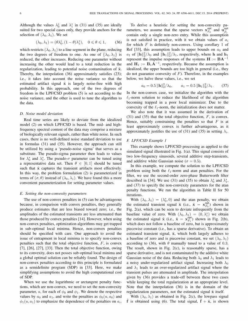
F. LPF/CSD Example 1This example shows LPF/CSD processing as applied to the
simulated signal illustrated in Fig. 1(a). This signal consists oftwo low-frequency sinusoids, several additive step-transients,and additive white Gaussian noise (σ = 0.5).
In this example, we compute the solution to the LPF/CSDproblem using both the `1-norm and atan penalties. For thefilter, we use the second-order zero-phase Butterworth filterdescribed in [34]. We use (31) and (35) to obtain λ∗0 and λ∗1,and (37) to specify the non-convexity parameters for the atanpenalty functions. We run the algorithm in Table II for 50iterations.
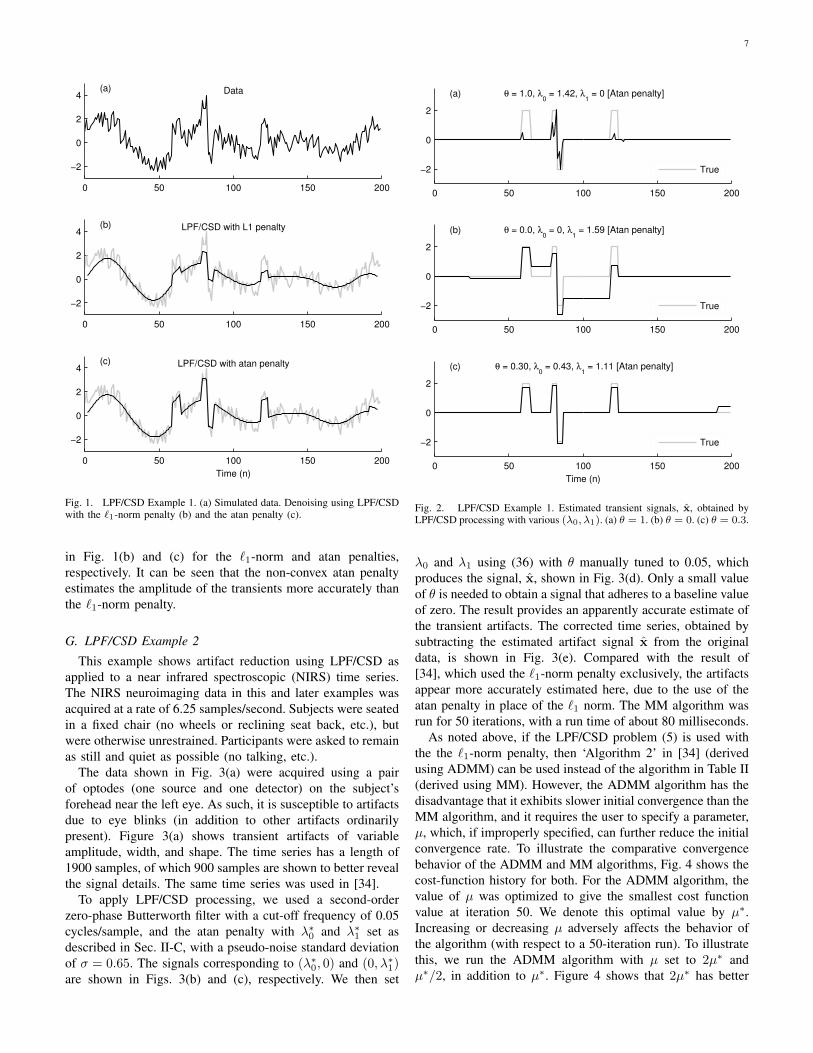
With (λ0, λ1) = (λ∗0, 0) and the atan penalty, we obtainthe estimated transient signal x (i.e., x = xopt
F0) shown in
Fig. 2(a), which can be seen to deviate infrequently from thebaseline value of zero. With (λ0, λ1) = (0, λ∗1) we obtainthe estimated signal x (i.e., x = xopt
F1) shown in Fig. 2(b),
which does not follow a baseline of zero, but is approximatelypiecewise constant (i.e., has a sparse derivative). To obtain anestimated transient signal, x, which both largely adheres toa baseline of zero and is piecewise constant, we set (λ0, λ1)according to (36), with θ manually tuned to a value of 0.3.The result, shown in Fig. 2(c), is reasonably sparse, has asparse derivative, and is not contaminated by the additive whiteGaussian noise of the data. Reducing both λ0 and λ1 leads toa noisy under-regularized artifact signal. Increasing both λ0and λ1 leads to an over-regularized artifact signal where thetransient pulses are attenuated in amplitude. The interpolationgiven by (36) provides a trade-off between these two caseswhile keeping the total regularization at an appropriate level.Note that the interpolation (36) is in the domain of theregularization parameters, not the estimated signal x itself.
With (λ0, λ1) as obtained in Fig. 2(c), the lowpass signalf is obtained using (6). The total signal, f + x, is shown
7
0 50 100 150 200
−2
0
2
4Data(a)
0 50 100 150 200
−2
0
2
4LPF/CSD with L1 penalty(b)
0 50 100 150 200
−2
0
2
4LPF/CSD with atan penalty
Time (n)
(c)
Fig. 1. LPF/CSD Example 1. (a) Simulated data. Denoising using LPF/CSDwith the `1-norm penalty (b) and the atan penalty (c).
in Fig. 1(b) and (c) for the `1-norm and atan penalties,respectively. It can be seen that the non-convex atan penaltyestimates the amplitude of the transients more accurately thanthe `1-norm penalty.
G. LPF/CSD Example 2
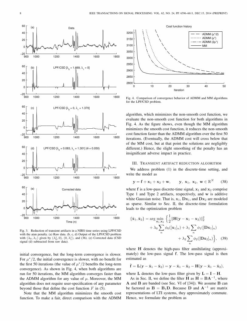
This example shows artifact reduction using LPF/CSD asapplied to a near infrared spectroscopic (NIRS) time series.The NIRS neuroimaging data in this and later examples wasacquired at a rate of 6.25 samples/second. Subjects were seatedin a fixed chair (no wheels or reclining seat back, etc.), butwere otherwise unrestrained. Participants were asked to remainas still and quiet as possible (no talking, etc.).
The data shown in Fig. 3(a) were acquired using a pairof optodes (one source and one detector) on the subject’sforehead near the left eye. As such, it is susceptible to artifactsdue to eye blinks (in addition to other artifacts ordinarilypresent). Figure 3(a) shows transient artifacts of variableamplitude, width, and shape. The time series has a length of1900 samples, of which 900 samples are shown to better revealthe signal details. The same time series was used in [34].
To apply LPF/CSD processing, we used a second-orderzero-phase Butterworth filter with a cut-off frequency of 0.05cycles/sample, and the atan penalty with λ∗0 and λ∗1 set asdescribed in Sec. II-C, with a pseudo-noise standard deviationof σ = 0.65. The signals corresponding to (λ∗0, 0) and (0, λ∗1)are shown in Figs. 3(b) and (c), respectively. We then set
0 50 100 150 200
−2
0
2
θ = 1.0, λ
0 = 1.42, λ
1 = 0 [Atan penalty](a)
True
0 50 100 150 200
−2
0
2
θ = 0.0, λ
0 = 0, λ
1 = 1.59 [Atan penalty](b)
True
0 50 100 150 200
−2
0
2
Time (n)
θ = 0.30, λ
0 = 0.43, λ
1 = 1.11 [Atan penalty](c)
True
Fig. 2. LPF/CSD Example 1. Estimated transient signals, x, obtained byLPF/CSD processing with various (λ0, λ1). (a) θ = 1. (b) θ = 0. (c) θ = 0.3.
λ0 and λ1 using (36) with θ manually tuned to 0.05, whichproduces the signal, x, shown in Fig. 3(d). Only a small valueof θ is needed to obtain a signal that adheres to a baseline valueof zero. The result provides an apparently accurate estimate ofthe transient artifacts. The corrected time series, obtained bysubtracting the estimated artifact signal x from the originaldata, is shown in Fig. 3(e). Compared with the result of[34], which used the `1-norm penalty exclusively, the artifactsappear more accurately estimated here, due to the use of theatan penalty in place of the `1 norm. The MM algorithm wasrun for 50 iterations, with a run time of about 80 milliseconds.
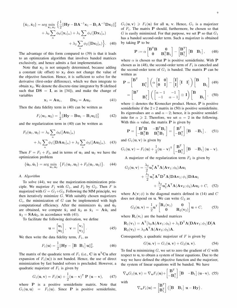
As noted above, if the LPF/CSD problem (5) is used withthe the `1-norm penalty, then ‘Algorithm 2’ in [34] (derivedusing ADMM) can be used instead of the algorithm in Table II(derived using MM). However, the ADMM algorithm has thedisadvantage that it exhibits slower initial convergence than theMM algorithm, and it requires the user to specify a parameter,µ, which, if improperly specified, can further reduce the initialconvergence rate. To illustrate the comparative convergencebehavior of the ADMM and MM algorithms, Fig. 4 shows thecost-function history for both. For the ADMM algorithm, thevalue of µ was optimized to give the smallest cost functionvalue at iteration 50. We denote this optimal value by µ∗.Increasing or decreasing µ adversely affects the behavior ofthe algorithm (with respect to a 50-iteration run). To illustratethis, we run the ADMM algorithm with µ set to 2µ∗ andµ∗/2, in addition to µ∗. Figure 4 shows that 2µ∗ has better
8 IEEE TRANSACTIONS ON SIGNAL PROCESSING. VOL. 62, NO. 24, PP. 6596–6611, DEC.15, 2014 (PREPRINT)
900 1000 1200 1400 1600 1800−20
0
20
40
60Data(a)
900 1000 1200 1400 1600 1800−20
0
20
40
60LPF/CSD [λ
0 = 1.669, λ
1 = 0](b)
900 1000 1200 1400 1600 1800−20
0
20
40
60LPF/CSD [λ
0 = 0, λ
1 = 1.370](c)
900 1000 1200 1400 1600 1800−20
0
20
40
60LPF/CSD [λ
0 = 0.083, λ
1 = 1.301] (θ = 0.050)(d)
900 1000 1200 1400 1600 1800−20
0
20
40
60
Time (n)
Corrected data(e)
Fig. 3. Reduction of transient artifacts in a NIRS time series using LPF/CSDwith the atan penalty. (a) Raw data. (b, c, d) Output of the LPF/CSD problemwith (λ0, λ1) given by (λ∗0, 0), (0, λ∗1), and (36). (e) Corrected data (CSDsignal (d) subtracted from raw data).
initial convergence, but the long-term convergence is slower.For µ∗/2, the initial convergence is slower, with no benefit forthe first 50 iterations (the value of µ∗/2 benefits the long-termconvergence). As shown in Fig. 4, when both algorithms arerun for 50 iterations, the MM algorithm converges faster thanthe ADMM algorithm for any value of µ. Moreover, the MMalgorithm does not require user-specification of any parameterbeyond those that define the cost function F in (5).
Note that the MM algorithm minimizes the smooth costfunction. To make a fair, direct comparison with the ADMM
0 10 20 30 40 502800
2850
2900
2950
3000
3050
3100
3150
3200
Iteration
Cost function history
ADMM (µ*/2)
ADMM (µ*)
ADMM (2µ*)
MM
Fig. 4. Comparison of convergence behavior of ADMM and MM algorithmsfor the LPF/CSD problem.
algorithm, which minimizes the non-smooth cost function, weevaluate the non-smooth cost function for both algorithms inFig. 4. As the figure shows, even though the MM algorithmminimizes the smooth cost function, it reduces the non-smoothcost function faster than the ADMM algorithm over the first 50iterations. (Eventually, the ADMM cost will cross below thatof the MM cost, but at that point the solutions are negligiblydifferent.) Hence, the slight smoothing of the penalty has aninsignificant adverse impact in practice.
III. TRANSIENT ARTIFACT REDUCTION ALGORITHM
We address problem (1) in the discrete-time setting, andwrite the model as
y = f + x1 + x2 + w, y, x1, x2, w ∈ RN (38)
where f is a low-pass discrete-time signal, x1 and x2 compriseType 1 and Type 2 artifacts, respectively, and w is additivewhite Gaussian noise. That is, x1, Dx1, and Dx2 are modeledas sparse. Similar to Sec. II, the discrete-time formulationleads to the optimization problem
{x1, x2} = arg minx1,x2
{12‖H(y − x1 − x2)‖22
+ λ0∑n
φ0([x1]n) + λ1∑n
φ1([Dx1]n)
+ λ2∑n
φ2([Dx2]n)}, (39)
where H denotes the high-pass filter annihilating (approxi-mately) the low-pass signal f . The low-pass signal is thenestimated as
f = L(y − x1 − x2) = y − x1 − x2 −H(y − x1 − x2),
where L denotes the low-pass filter given by L = I−H.As in Sec. II, we define the filter H as H = BA−1, where
A and B are banded (see Sec. VI of [34]). We assume B canbe factored as B = B1D. Because D and A−1 are matrixrepresentations of LTI systems, they approximately commute.Hence, we formulate the problem as
9
{x1, x2} = arg minx1,x2
{12‖Hy−BA−1x1−B1A
−1Dx2‖22
+ λ0∑n
φ0([x1]n) + λ1∑n
φ1([Dx1]n)
+ λ2∑n
φ2([Dx2]n)}. (40)
The advantage of this form compared to (39) is that it leadsto an optimization algorithm that involves banded matricesexclusively, and hence admits a fast implementation.
Note that x2 is not uniquely determined, because addinga constant (dc offset) to x2 does not change the value ofthe objective function. Hence, it is sufficient to solve for thederivative (first-order difference), which we then integrate toobtain x2. We denote the discrete-time integrator by S (definedsuch that DS = I, as in [34]), and make the change ofvariables
x1 = Au1, Dx2 = Au2. (41)
Then the data fidelity term in (40) can be written as
F1(u1,u2) =1
2‖Hy −Bu1 −B1u2‖22 (42)
and the regularization term in (40) can be written as
F2(u1,u2) = λ0∑n
φ0([Au1]n)
+ λ1∑n
φ1([DAu1]n) + λ2∑n
φ2([Au2]n). (43)
Then F = F1 + F2, and in terms of u1 and u2 we have theoptimization problem
{u0, u1} = arg minu1,u2
{F1(u1,u2) + F2(u1,u2)
}. (44)
A. Algorithm
To solve (44), we use the majorization-minimization prin-ciple. We majorize F1 with G1, and F2 by G2. Then F ismajorized with G = G1+G2. Following the MM principle, wethen iteratively minimize G. With suitably chosen majorizersGi, the minimization of G can be implemented with highcomputational efficiency. After the minimizers u1 and u2
are obtained, we compute x1 and x2 as x1 = Au1 andx2 = SAu2, in accordance with (41).
To facilitate the following derivation, we define
u =
[u1
u2
], v =
[v1
v2
]. (45)
We then write the data fidelity term, F1, as
F1(u) =1
2‖Hy −
[B B1
]u‖22. (46)
The matrix of the quadratic term of F1 (i.e., C in uTCu afterexpansion of F1(u)) is not banded. Hence, the use of directminimization by fast banded solvers is precluded. However, aquadratic majorizer of F1 is given by
G1(u,v) = F1(u) +1
2(u− v)T P (u− v), (47)
where P is a positive semidefinite matrix. Note thatG1(u,u) = F1(u). Since P is positive semidefinite,
G1(u,v) > F1(u) for all u, v. Hence, G1 is a majorizerof F1. The matrix P should, furthermore, be chosen so thatG is easily minimized. For that purpose, we set P so that G1
has a banded second-order term. Such a majorizer is obtainedby taking P to be
P := α
[BTB 0
0 BT1B1
]−[BT
BT1
] [B B1
], (48)
where α is chosen so that P is positive semidefinite. With Pchosen as in (48), the second-order term of F1 is canceled andthe second-order term of G1 is banded. The matrix P can bewritten as
P =
[BT
BT1
](α
[I 00 I
]−[II
] [I I
]) [BB1
](49)
=
[BT
BT1
]([α− 1 −1−1 α− 1
]⊗ I
)[B
B1
], (50)
where ⊗ denotes the Kronecker product. Hence, P is positivesemidefinite if the 2×2 matrix in (50) is positive semidefinite.Its eigenvalues are α and α− 2; hence, it is positive semidef-inite for α > 2. Therefore, we set α = 2 in the following.With this α value, the matrix P is given by
P =
[BTB −BTB1
−BT1B BT
1B1
]=
[BT
−BT1
] [B −B1
], (51)
and G1(u,v) is given by
G1(u,v) = F1(u) +1
2(u− v)T
[BT
−BT1
] [B −B1
](u− v).
A majorizer of the regularization term F2 is given by
G2(u,v) =λ02
uT1ATΛ(Av1;φ0)Au1
+λ12
uT1ATDTΛ(DAv1;φ1)DAu1
+λ22
uT2ATΛ(Av2;φ2)Au2 + C, (52)
where Λ(v;φ) is the diagonal matrix defined in (14) and Cdoes not depend on u. We can write G2 as
G2(u,v) =1
2uT
[R1(v1) 0
0 R2(v2)
]u + C, (53)
where Ri(vi) are the banded matrices
R1(v1) = AT[λ0Λ(Av1;φ0) + λ1DTΛ(DAv1;φ1)D]A
R2(v2) = λ2ATΛ(Av2;φ2)A.
Consequently, a quadratic majorizer of F is given by
G(u,v) = G1(u,v) +G2(u,v). (54)
To find u minimizing G, we set to zero the gradient of G withrespect to u, to obtain a system of linear equations. Due to theway we have defined the objective function and the majorizer,the system of linear equations will be banded. We have
∇uG1(u,v) = ∇uF1(u)+
[BT
−BT1
] [B −B1
](u−v), (55)
with∇uF1(u) =
[BT
BT1
] ([B B1
]u−Hy
).
10 IEEE TRANSACTIONS ON SIGNAL PROCESSING. VOL. 62, NO. 24, PP. 6596–6611, DEC.15, 2014 (PREPRINT)
TABLE IIITRANSIENT ARTIFACT REDUCTION ALGORITHM (TARA)
Input: y ∈ RN, λi > 0, φi,A,B
1. y1 = BTBA−1y (BTHy )
2. y2 = BT1BA−1y (BT
1Hy )3. u1 = 0, u2 = 0 (initialization)
Repeat4. [Λ0]n,n = λ0/ψ0([Au1]n) (Λ0 is diagonal)5. [Λ1]n,n = λ1/ψ1([DAu1]n) (Λ1 is diagonal)6. [Λ2]n,n = λ2/ψ2([Au2]n) (Λ2 is diagonal)
7. Q1 = 2BTB + AT(Λ0 + DTΛ1D)A (Q1 is banded)
8. Q2 = 2BT1B1 + ATΛ2A (Q2 is banded)
9. g = Bu1 −B1u2
10. u1 = Q−11
(y1 + BTg
)11. u2 = Q−1
2
(y2 −BT
1g)
Until convergence12. x1 = Au1, x2 = SAu2
Output: x1, x2
We also have
∇uG2(u,v) =
[R1(v1) 0
0 R2(v2)
]u. (56)
Hence, ∇uG = ∇uG1+∇uG2 = 0 leads to the linear system[2BTB + R1(v1) 0
0 2BT1B1 + R2(v2)
] [u1
u2
]=
[BT
BT1
]Hy +
[BT
−BT1
] [B −B1
] [v1
v2
]. (57)
Note that the system matrix is banded. The solution to (57) isgiven by
g = Bv1 −B1v2 (58)
u1 =[2BTB + R1(v1)
]−1 (BTHy + BTg
)(59)
u2 =[2BT
1B1 + R2(v2)]−1 (
BT1Hy −BT
1g). (60)
Hence, minimizing the majorizer G according to the MMupdate equation (17) leads to
g(i) = Bu(i)1 −B1u
(i)2 (61)
u(i+1)1 =
[2BTB + R1(u
(i)1 )]−1 (
BTHy + BTg(i))
(62)
u(i+1)2 =
[2BT
1B1 + R2(u(i)2 )]−1 (
BT1Hy −BT
1g(i))
(63)
Equations (61)-(63) constitute the iterative algorithm,TARA, summarized in Table III. Note that the system matricesare banded; hence, the algorithm can be implemented usingfast solvers for banded systems. The vectors BTHy andBT
1Hy need to be computed one time only. The algorithmdoes not require any parameters other than the ones in (40).After u1 and u2 are obtained upon convergence of thealgorithm, x1 and x2 are obtained using (41).
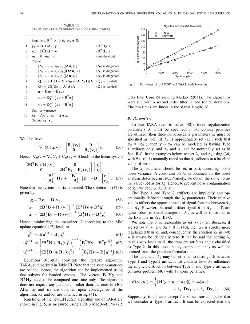
Run times of the new LPF/CSD algorithm and of TARA areshown in Fig. 5, as measured using a 2013 MacBook Pro (2.5
0 1000 2000 3000 4000 50000
50
100
150
200
250
300
350
Signal length
Run tim
e (
mill
iseconds)
Algorithm run time (50 iterations)
TARA
LPF/CSD
Fig. 5. Run times of LPF/CSD and TARA with linear fits.
GHz Intel Core i5) running Matlab R2011a. The algorithmswere run with a second order filter H and for 50 iterations.The run times are linear in the signal length, N .
B. Parameters
To use TARA (i.e., to solve (40)), three regularizationparameters λi must be specified; if non-convex penaltiesare utilized, then three non-convexity parameters ai must bespecified as well. If λ2 is appropriately set (i.e., such thatx2 ≈ x2 ), then y − x2 can be modeled as having Type1 artifacts only, and λ0 and λ1 can be nominally set as inSec. II-C. In the examples below, we set λ0 and λ1 using (36)with θ ∈ (0, 1) manually tuned so that x0 adheres to a baselinevalue of zero.
The λ2 parameter should be set, in part, according to thenoise variance. A constraint on λ2 is obtained via the noiseanalysis described in II-C. Namely, we obtain the same nomi-nal value (35) as for λ∗1. Hence, to prevent noise contaminationof x2, we require λ2 > λ∗1.
The Type 1 and Type 2 artifacts are implicitly and op-erationally defined through the λi parameters. Their relativevalues affects the apportionment of signal features between x1
and x2. However, the total artifact signal x1 + x2, and f , arequite robust to small changes in λi, as will be illustrated inthe Example in Sec. III-C.
We note that it is reasonable to set λ2 > λ1. Because, ifwe set λ2 6 λ1 and λ0 > 0 in (40), then x1 is strictly moreregularized than x2 and, consequently, the solution x1 in (40)will always be identically zero. It can be said that setting λiin this way leads to all the transient artifacts being classifiedas Type 2. In this case, the x1 component may as well beomitted from the problem formulation.
The parameter λ2 may be set so as to distinguish betweenType 1 and Type 2 artifacts. To consider how λ2 influencesthe implicit distinction between Type 1 and Type 2 artifacts,consider problem (40) with `1 norm penalties,
F (x1,x2) =1
2‖H(y − x1 − x2)‖22 + λ0‖x1‖1
+ λ1‖Dx1‖1 + λ2‖Dx2‖1. (64)
Suppose y is all zero except for some transient pulse thatwe consider a Type 1 artifact. It can be expected that the
11
minimizer of F is likewise some transient pulse, which wedenote by p; i.e., x1 + x2 = p. If p is considered a Type 1artifact, then λi should be set so that x1 = p and x2 = 0. Tofind a rule for setting the parameter values, we evaluate theobjective function F for two candidate solutions:
S1 = {x1 = p, x2 = 0}, S2 = {x1 = 0, x2 = p}. (65)
If S1 minimizes F , then TARA correctly classifies p as a Type1 artifact; while if S2 minimizes F , then TARA incorrectlyclassifies p as a Type 2 artifact. Solution S1 can be the optimalsolution only if F (S1) < F (S2). Because (x1 + x2) is thesame for solutions S1 and S2, the data fidelity term of F isequal for S1 and S2. Hence, the relative cost depends only onthe penalty terms. Therefore, we have
λ0‖p‖1 + λ1‖Dp‖1S1
≶S2
λ2‖Dp‖1 (66)
orλ0‖p‖1‖Dp‖1
+ λ1S1
≶S2
λ2. (67)
The notation ≶ means S1 is the optimal solution if the left-hand side is the smaller value, while S2 is optimal if theright-hand side is smaller. Hence, for p to be classified asa Type 1 artifact by TARA, λ2 must be at least as great asthe quantity on the left-hand side of (67). Note that condition(67) is invariant to amplitude scaling of p; i.e., only the shapeof p matters.
As an example, suppose that p is taken to be a rectangularpulse of length M samples and amplitude A. Then ‖p‖1 =MA and ‖Dp‖1 = 2A, so condition (67) can be written as
0.5Mλ0 + λ1S1
≶S2
λ2. (68)
Hence, for the M -point pulse to be exhibited in x1, theparameter λ2 must exceed λ1 by 0.5Mλ0. When (λ0, λ1) =(θλ∗0, (1 − θ)λ∗1), as suggested in (36), then (68) gives acondition in terms of θ,
θ(0.5Mλ∗0 − λ∗1) + λ∗1S1
≶S2
λ2. (69)
We noted above that λ2 should satisfy λ2 > λ∗1. Hence, λ2should be set according to
λ2 > max{λ∗1, λ∗1 + θ(0.5Mλ∗0 − λ∗1)}. (70)
It experiments, we have found that 0.5Mλ∗0 − λ∗1 is usuallypositive, so the second term in (70) dominates. Moreover, θ isoften relatively small in practice (sufficient so that x1 adheresto a baseline of zero). Hence, it will often be sufficient thatλ2 be only slightly larger than λ∗1. The use of condition (68)to control the behavior of TARA is illustrated in Sec. III-C.
Based on the forgoing considerations, we suggest writingλ2 = βλ∗1 and taking β as a tuning parameter with a nominalrange of β ∈ [1, 2]. In conjunction with the discussion inSec. II-D, we obtain a parameterization of the TARA problem(40) in terms of (σ, θ, β) instead of (λ0, λ1, λ2). We findthis parameterization more useful in practice because theinfluence of each parameter can be more readily understood.
0 50 100 150 200
−3−2−1
0123
−2−1
01
0
−1012
−3−2−1
0123
y
x1
x2
f
Total
Time (n)
(a)
0 50 100 150 200
−3−2−1
0123
−1012
−2−1
012
012
−3−2−1
0123
y
x1
x2
f
Total
Time (n)
(b)
Fig. 6. Signal decomposition and filtering with TARA. (a) Pulses 4 samplesand shorter appear in x1. (b) Pulses 4 samples and longer appear in x2.
In particular, we consider (θ, β) to be shape parameters; theyinfluence the shape of the estimated transients.
When non-convex penalties are utilized, a0 and a1 canbe set as in (37). Following the same considerations as inSec. II-E, we set a2 = 0.5 ‖h1‖22/λ2 like for a1.
C. TARA Example 1
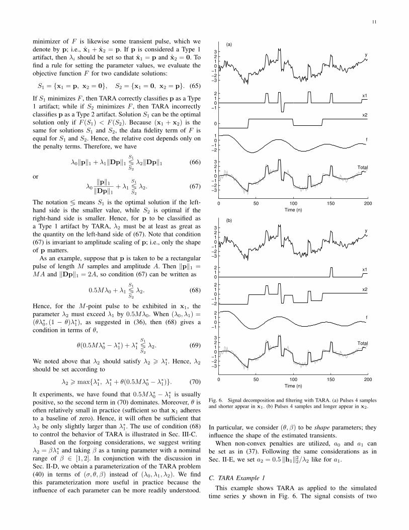
This example shows TARA as applied to the simulatedtime series y shown in Fig. 6. The signal consists of two
12 IEEE TRANSACTIONS ON SIGNAL PROCESSING. VOL. 62, NO. 24, PP. 6596–6611, DEC.15, 2014 (PREPRINT)
low-frequency sinusoids, several additive rectangular pulsesof short duration, several additive step discontinuities, and ad-ditive white Gaussian noise (σ = 0.3). Each of the rectangularpulses has a length of four samples, except for the last pulse(at n = 150) which has a length of three samples.
In this example, we use a fourth-order zero-phase Butter-worth filter with fc = 0.03 cycles/sample. We also use thenon-convex atan penalty, set λ∗0 and λ∗1 according to (31) and(35) in Sec. II-C, and set θ = 0.3 by manual tuning as inSec. II-F.
To demonstrate the influence of λ2 as discussed inSec. III-B, we consider the question of how to set λ2 to ensurethat the brief rectangular pulses appear in x1 rather than inx2 (i.e., to ensure TARA classifies these pulses as Type 1artifacts). Since all the brief pulses are of length 4 or less, weset M = 4 in (68) to find that 2λ0 + λ1 is the critical valuefor λ2. Hence, we must set λ2 > 2λ0 + λ1 to ensure that thepulses appear in x1. Therefore, we set λ2 = 1.1× (2λ0+λ1);i.e., β = 1.1. The output of TARA for this λ2 is shown inFig. 6(a). In conformity with our expectation, all the briefpulses are exhibited in x1, i.e., they are classified by TARAas Type 1 artifacts. The signal x2 is piecewise constant andcontains no brief pulses. (The small step at the end of x1 isa boundary artifact due to applying the recursive filter H to afinite-length signal.)
To further illustrate the role of λ2, we set λ2 = 0.9 ×(2λ0+λ1). This value is less than the critical value needed toclassify a length-4 pulse as a Type 1 artifact. Accordingly, it isexpected that TARA will classify pulses of length 4 and longeras Type 2 artifacts and that they will be exhibited in x2. Theoutput of TARA for this value of λ2 is shown in Fig. 6(b). Aspredicted, the length-4 pulses are exhibited in x2. The onlypulse exhibited in x1 is the final one (at n = 150), whichis of length 3. This example validates the use of λ2 for thedisambiguation of pulses based on their duration.
This example uses rectangular pulses because of the avail-ability of the simple formula (68). TARA does not explicitlymodel a signal in terms of rectangular pulses, and its effective-ness is not limited to rectangular artifacts. For real data withtransient artifacts of complex shape, it is not expected that asimple formula for a critical value will be available; however,the general influence of λ2 on the relative properties of x1 andx2 holds. Namely, decreasing λ2 results in more waveformsbeing classified as Type 2 artifacts.
Note that the low-pass signal, f , is essentially the same inFigs. 6(a) and 6(b). Likewise, the total signal, x = x1+x2+ f ,is approximately the same in both figures. The small changein λ2 produced only a small change in the total signal, eventhough it produced a large change in xi. Hence, for the purposeof denoising, the total signal is not overly sensitive to the exactvalue of λ2. Note that TARA provides a reasonable denoisingresult: the total signal is relatively noise-free, preserves thediscontinuities in the data, and does not exhibit ringing aroundthe discontinuities.
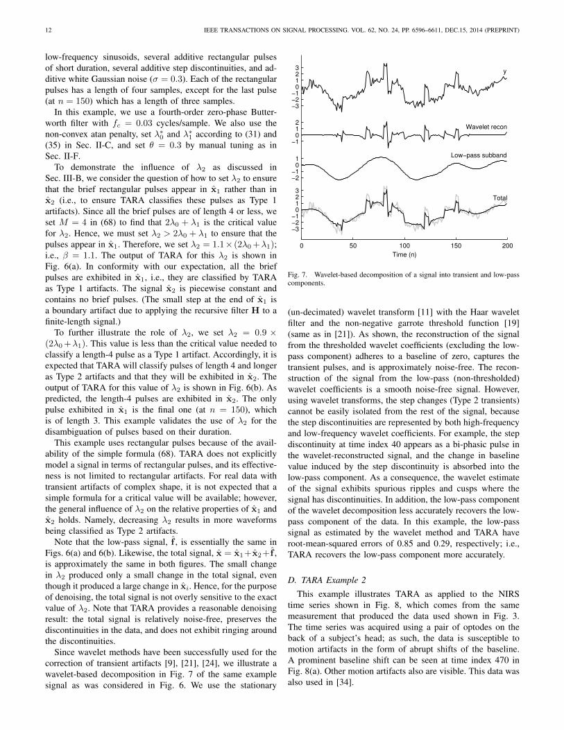
Since wavelet methods have been successfully used for thecorrection of transient artifacts [9], [21], [24], we illustrate awavelet-based decomposition in Fig. 7 of the same examplesignal as was considered in Fig. 6. We use the stationary
0 50 100 150 200
−3−2−1
0123
−2−1
01
−1012
−3−2−1
0123
y
Wavelet recon
Low−pass subband
Total
Time (n)
Fig. 7. Wavelet-based decomposition of a signal into transient and low-passcomponents.
(un-decimated) wavelet transform [11] with the Haar waveletfilter and the non-negative garrote threshold function [19](same as in [21]). As shown, the reconstruction of the signalfrom the thresholded wavelet coefficients (excluding the low-pass component) adheres to a baseline of zero, captures thetransient pulses, and is approximately noise-free. The recon-struction of the signal from the low-pass (non-thresholded)wavelet coefficients is a smooth noise-free signal. However,using wavelet transforms, the step changes (Type 2 transients)cannot be easily isolated from the rest of the signal, becausethe step discontinuities are represented by both high-frequencyand low-frequency wavelet coefficients. For example, the stepdiscontinuity at time index 40 appears as a bi-phasic pulse inthe wavelet-reconstructed signal, and the change in baselinevalue induced by the step discontinuity is absorbed into thelow-pass component. As a consequence, the wavelet estimateof the signal exhibits spurious ripples and cusps where thesignal has discontinuities. In addition, the low-pass componentof the wavelet decomposition less accurately recovers the low-pass component of the data. In this example, the low-passsignal as estimated by the wavelet method and TARA haveroot-mean-squared errors of 0.85 and 0.29, respectively; i.e.,TARA recovers the low-pass component more accurately.
D. TARA Example 2
This example illustrates TARA as applied to the NIRStime series shown in Fig. 8, which comes from the samemeasurement that produced the data used shown in Fig. 3.The time series was acquired using a pair of optodes on theback of a subject’s head; as such, the data is susceptible tomotion artifacts in the form of abrupt shifts of the baseline.A prominent baseline shift can be seen at time index 470 inFig. 8(a). Other motion artifacts also are visible. This data wasalso used in [34].
13
0 200 400 600 800 1000 1200 1400 1600 1800
−20
−10
0
0
10
20
0
10
0
10
20
0
10
20
Raw data
Type 1 artifact
Type 2 artifact
Total artifact
Corrected data
Time (n)
Fig. 8. Artifact reduction with TARA using the atan penalty, as applied toa NIRS time series.
To apply TARA for artifact suppression, we must specify thefilter H, the three regularization parameters, and the penaltyfunctions. We used a second-order zero-phase Butterworthfilter with fc = 0.06 cycles/sample. The tuning proceduredescribed in Sec. II-D was used to set λ∗0 and λ∗1 with a pseudo-noise standard deviation of σ = 0.25. We manually tuned theshape parameters to θ = 0.05 and β = 1.4. The atan penaltywas used, with non-convexity parameters set according to (37).We ran TARA for 100 iterations with a run time of about 0.28seconds.
The Type 1 and Type 2 artifact signals estimated by TARA,x1 and x2, shown in Fig. 8, are sparse and approximatelypiecewise constant, as intended. The estimated total artifactsignal, x1 + x2, which comprises additive step discontinuitiesand transient spikes, appears to accurately model the artifactspresent in the data. Note that the corrected time series,obtained by subtracting the total estimated artifact signal fromthe original time series, has both low-frequency and high-frequency spectral content. Compared with [34], in whichLPF/TVD processing is applied to the same data, the artifactsappear to be more accurately estimated here.
E. Wavelet-based artifact reduction
It has been found that wavelet methods compare favorably toother methods for the correction of motion artifacts in single-channel NIRS time series [9], [21], [24]. Figure 9 compareswavelet transient artifact reduction (WATAR) and TARA asapplied to the NIRS data from Fig. 8. As in [21], we usethe stationary (un-decimated) wavelet transform [11] with theHaar wavelet filter and the non-negative garrote threshold
1200 1300 1400 1500 1600 1700
Time (n)
Raw data
Artifact (wavelet)
Artifact (TARA)
Corrected (wavelet)
Corrected (TARA)
Fig. 9. Artifact estimation and correction using wavelets and TARA.
function [19]. We apply thresholding to all subbands exceptthe low-pass one. The wavelet-corrected time series does nothave the long-term drift that the TARA-corrected time serieshas; however, that is easily removed by LTI filtering andits removal is not an objective of TARA. Moreover, somebiological information may be present at low frequencies (seeSec. III-G).
It can be seen that both methods otherwise give generallysimilar results, but the TARA-estimated artifact signal capturesabrupt changes in the data, unlike the wavelet-estimated arti-fact signal. The artifact in the interval 1370-1420 is estimatedby TARA with distinct pre- and post-artifact baseline values,while the wavelet-estimated artifact signal exhibits a smallchange due to the slowly-varying low-pass component (comingfrom the low-pass subband of the wavelet transform). Inaddition, TARA finds an abrupt change at time index 1530,while the wavelet method exhibits only a small bi-phasic (zero-mean) pulse at that instant. TARA is better able to estimateabrupt step changes than the wavelet method because it isexplicitly based on a two-component model. In NIRS timeseries analysis, motion artifacts often cause step changes, andthis motivates the accurate estimation thereof.
That TARA and wavelet methods give similar results can beexplained by their being based on similar underlying models.The wavelet method implicitly models transient artifacts aspiecewise smooth. TARA is based on a similar model, butuses an optimization approach instead of a fixed transform.
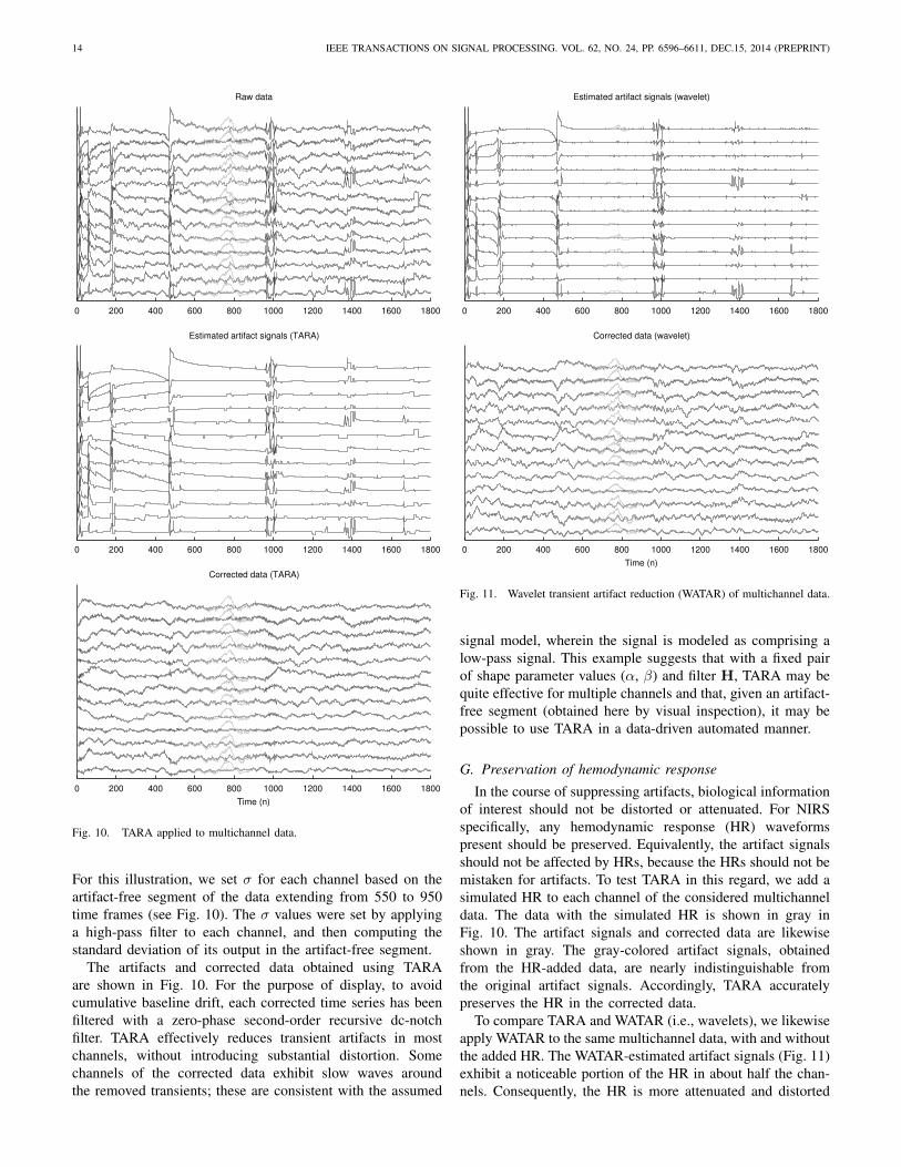
F. Multichannel data
Physiological time-series data (e.g., NIRS, EEG) are oftenacquired in multichannel form. If different regularization pa-rameters are to be required for each channel, then setting theparameters will be a problematic issue. In this example, weapply TARA to multichannel data (Fig. 10, black) and use thesame shape parameters (α, β) and filter H for all channels. Thepsuedo-noise parameter σ should, however, be set channel-by-channel, because the channels are not equally normalized.
14 IEEE TRANSACTIONS ON SIGNAL PROCESSING. VOL. 62, NO. 24, PP. 6596–6611, DEC.15, 2014 (PREPRINT)
0 200 400 600 800 1000 1200 1400 1600 1800
Raw data
0 200 400 600 800 1000 1200 1400 1600 1800
Estimated artifact signals (TARA)
0 200 400 600 800 1000 1200 1400 1600 1800
Corrected data (TARA)
Time (n)
Fig. 10. TARA applied to multichannel data.
For this illustration, we set σ for each channel based on theartifact-free segment of the data extending from 550 to 950time frames (see Fig. 10). The σ values were set by applyinga high-pass filter to each channel, and then computing thestandard deviation of its output in the artifact-free segment.
The artifacts and corrected data obtained using TARAare shown in Fig. 10. For the purpose of display, to avoidcumulative baseline drift, each corrected time series has beenfiltered with a zero-phase second-order recursive dc-notchfilter. TARA effectively reduces transient artifacts in mostchannels, without introducing substantial distortion. Somechannels of the corrected data exhibit slow waves aroundthe removed transients; these are consistent with the assumed
0 200 400 600 800 1000 1200 1400 1600 1800
Estimated artifact signals (wavelet)
0 200 400 600 800 1000 1200 1400 1600 1800
Corrected data (wavelet)
Time (n)
Fig. 11. Wavelet transient artifact reduction (WATAR) of multichannel data.
signal model, wherein the signal is modeled as comprising alow-pass signal. This example suggests that with a fixed pairof shape parameter values (α, β) and filter H, TARA may bequite effective for multiple channels and that, given an artifact-free segment (obtained here by visual inspection), it may bepossible to use TARA in a data-driven automated manner.
G. Preservation of hemodynamic response
In the course of suppressing artifacts, biological informationof interest should not be distorted or attenuated. For NIRSspecifically, any hemodynamic response (HR) waveformspresent should be preserved. Equivalently, the artifact signalsshould not be affected by HRs, because the HRs should not bemistaken for artifacts. To test TARA in this regard, we add asimulated HR to each channel of the considered multichanneldata. The data with the simulated HR is shown in gray inFig. 10. The artifact signals and corrected data are likewiseshown in gray. The gray-colored artifact signals, obtainedfrom the HR-added data, are nearly indistinguishable fromthe original artifact signals. Accordingly, TARA accuratelypreserves the HR in the corrected data.
To compare TARA and WATAR (i.e., wavelets), we likewiseapply WATAR to the same multichannel data, with and withoutthe added HR. The WATAR-estimated artifact signals (Fig. 11)exhibit a noticeable portion of the HR in about half the chan-nels. Consequently, the HR is more attenuated and distorted
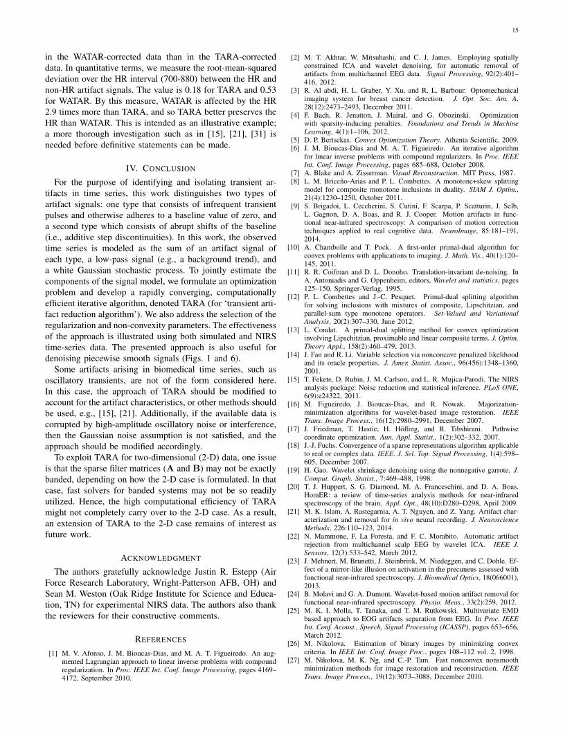
15
in the WATAR-corrected data than in the TARA-correcteddata. In quantitative terms, we measure the root-mean-squareddeviation over the HR interval (700-880) between the HR andnon-HR artifact signals. The value is 0.18 for TARA and 0.53for WATAR. By this measure, WATAR is affected by the HR2.9 times more than TARA, and so TARA better preserves theHR than WATAR. This is intended as an illustrative example;a more thorough investigation such as in [15], [21], [31] isneeded before definitive statements can be made.
IV. CONCLUSION
For the purpose of identifying and isolating transient ar-tifacts in time series, this work distinguishes two types ofartifact signals: one type that consists of infrequent transientpulses and otherwise adheres to a baseline value of zero, anda second type which consists of abrupt shifts of the baseline(i.e., additive step discontinuities). In this work, the observedtime series is modeled as the sum of an artifact signal ofeach type, a low-pass signal (e.g., a background trend), anda white Gaussian stochastic process. To jointly estimate thecomponents of the signal model, we formulate an optimizationproblem and develop a rapidly converging, computationallyefficient iterative algorithm, denoted TARA (for ‘transient arti-fact reduction algorithm’). We also address the selection of theregularization and non-convexity parameters. The effectivenessof the approach is illustrated using both simulated and NIRStime-series data. The presented approach is also useful fordenoising piecewise smooth signals (Figs. 1 and 6).
Some artifacts arising in biomedical time series, such asoscillatory transients, are not of the form considered here.In this case, the approach of TARA should be modified toaccount for the artifact characteristics, or other methods shouldbe used, e.g., [15], [21]. Additionally, if the available data iscorrupted by high-amplitude oscillatory noise or interference,then the Gaussian noise assumption is not satisfied, and theapproach should be modified accordingly.
To exploit TARA for two-dimensional (2-D) data, one issueis that the sparse filter matrices (A and B) may not be exactlybanded, depending on how the 2-D case is formulated. In thatcase, fast solvers for banded systems may not be so readilyutilized. Hence, the high computational efficiency of TARAmight not completely carry over to the 2-D case. As a result,an extension of TARA to the 2-D case remains of interest asfuture work.
ACKNOWLEDGMENT
The authors gratefully acknowledge Justin R. Estepp (AirForce Research Laboratory, Wright-Patterson AFB, OH) andSean M. Weston (Oak Ridge Institute for Science and Educa-tion, TN) for experimental NIRS data. The authors also thankthe reviewers for their constructive comments.
REFERENCES
[1] M. V. Afonso, J. M. Bioucas-Dias, and M. A. T. Figueiredo. An aug-mented Lagrangian approach to linear inverse problems with compoundregularization. In Proc. IEEE Int. Conf. Image Processing, pages 4169–4172, September 2010.
[2] M. T. Akhtar, W. Mitsuhashi, and C. J. James. Employing spatiallyconstrained ICA and wavelet denoising, for automatic removal ofartifacts from multichannel EEG data. Signal Processing, 92(2):401–416, 2012.
[3] R. Al abdi, H. L. Graber, Y. Xu, and R. L. Barbour. Optomechanicalimaging system for breast cancer detection. J. Opt. Soc. Am. A,28(12):2473–2493, December 2011.
[4] F. Bach, R. Jenatton, J. Mairal, and G. Obozinski. Optimizationwith sparsity-inducing penalties. Foundations and Trends in MachineLearning, 4(1):1–106, 2012.
[5] D. P. Bertsekas. Convex Optimization Theory. Athenta Scientific, 2009.[6] J. M. Bioucas-Dias and M. A. T. Figueiredo. An iterative algorithm
for linear inverse problems with compound regularizers. In Proc. IEEEInt. Conf. Image Processing, pages 685–688, October 2008.
[7] A. Blake and A. Zisserman. Visual Reconstruction. MIT Press, 1987.[8] L. M. Briceno-Arias and P. L. Combettes. A monotone+skew splitting
model for composite monotone inclusions in duality. SIAM J. Optim.,21(4):1230–1250, October 2011.
[9] S. Brigadoi, L. Ceccherini, S. Cutini, F. Scarpa, P. Scatturin, J. Selb,L. Gagnon, D. A. Boas, and R. J. Cooper. Motion artifacts in func-tional near-infrared spectroscopy: A comparison of motion correctiontechniques applied to real cognitive data. NeuroImage, 85:181–191,2014.
[10] A. Chambolle and T. Pock. A first-order primal-dual algorithm forconvex problems with applications to imaging. J. Math. Vis., 40(1):120–145, 2011.
[11] R. R. Coifman and D. L. Donoho. Translation-invariant de-noising. InA. Antoniadis and G. Oppenheim, editors, Wavelet and statistics, pages125–150. Springer-Verlag, 1995.
[12] P. L. Combettes and J.-C. Pesquet. Primal-dual splitting algorithmfor solving inclusions with mixtures of composite, Lipschitzian, andparallel-sum type monotone operators. Set-Valued and VariationalAnalysis, 20(2):307–330, June 2012.
[13] L. Condat. A primal-dual splitting method for convex optimizationinvolving Lipschitzian, proximable and linear composite terms. J. Optim.Theory Appl., 158(2):460–479, 2013.
[14] J. Fan and R. Li. Variable selection via nonconcave penalized likelihoodand its oracle properties. J. Amer. Statist. Assoc., 96(456):1348–1360,2001.
[15] T. Fekete, D. Rubin, J. M. Carlson, and L. R. Mujica-Parodi. The NIRSanalysis package: Noise reduction and statistical inference. PLoS ONE,6(9):e24322, 2011.
[16] M. Figueiredo, J. Bioucas-Dias, and R. Nowak. Majorization-minimization algorithms for wavelet-based image restoration. IEEETrans. Image Process., 16(12):2980–2991, December 2007.
[17] J. Friedman, T. Hastie, H. Hofling, and R. Tibshirani. Pathwisecoordinate optimization. Ann. Appl. Statist., 1(2):302–332, 2007.
[18] J.-J. Fuchs. Convergence of a sparse representations algorithm applicableto real or complex data. IEEE. J. Sel. Top. Signal Processing, 1(4):598–605, December 2007.
[19] H. Gao. Wavelet shrinkage denoising using the nonnegative garrote. J.Comput. Graph. Statist., 7:469–488, 1998.
[20] T. J. Huppert, S. G. Diamond, M. A. Franceschini, and D. A. Boas.HomER: a review of time-series analysis methods for near-infraredspectroscopy of the brain. Appl. Opt., 48(10):D280–D298, April 2009.
[21] M. K. Islam, A. Rastegarnia, A. T. Nguyen, and Z. Yang. Artifact char-acterization and removal for in vivo neural recording. J. NeuroscienceMethods, 226:110–123, 2014.
[22] N. Mammone, F. La Foresta, and F. C. Morabito. Automatic artifactrejection from multichannel scalp EEG by wavelet ICA. IEEE J.Sensors, 12(3):533–542, March 2012.
[23] J. Mehnert, M. Brunetti, J. Steinbrink, M. Niedeggen, and C. Dohle. Ef-fect of a mirror-like illusion on activation in the precuneus assessed withfunctional near-infrared spectroscopy. J. Biomedical Optics, 18(066001),2013.
[24] B. Molavi and G. A. Dumont. Wavelet-based motion artifact removal forfunctional near-infrared spectroscopy. Physio. Meas., 33(2):259, 2012.
[25] M. K. I. Molla, T. Tanaka, and T. M. Rutkowski. Multivariate EMDbased approach to EOG artifacts separation from EEG. In Proc. IEEEInt. Conf. Acoust., Speech, Signal Processing (ICASSP), pages 653–656,March 2012.
[26] M. Nikolova. Estimation of binary images by minimizing convexcriteria. In IEEE Int. Conf. Image Proc., pages 108–112 vol. 2, 1998.
[27] M. Nikolova, M. K. Ng, and C.-P. Tam. Fast nonconvex nonsmoothminimization methods for image restoration and reconstruction. IEEETrans. Image Process., 19(12):3073–3088, December 2010.
16 IEEE TRANSACTIONS ON SIGNAL PROCESSING. VOL. 62, NO. 24, PP. 6596–6611, DEC.15, 2014 (PREPRINT)
[28] J.-C. Pesquet and N. Pustelnik. A parallel inertial proximal optimizationmethod. Pacific J. Optimization, 8(2):273–305, April 2012.
[29] W. H. Press, S. A. Teukolsky, W. T. Vetterling, and B. P. Flannery.Numerical recipes in C: the art of scientific computing (2nd ed.).Cambridge University Press, 1992.
[30] H. Raguet, J. Fadili, and G. Peyre. A generalized forward-backwardsplitting. SIAM J. Imag. Sci., 6(3):1199–1226, 2013.
[31] F. C. Robertson, T. S. Douglas, and E. M. Meintjes. Motion artifactremoval for functional near infrared spectroscopy: A comparison ofmethods. IEEE Trans. Biomed. Eng., 57(6):1377–1387, June 2010.
[32] H. Sato, N. Tanaka, M. Uchida, Y. Hirabayashi, M. Kanai, T. Ashida,I. Konishi, and A. Maki. Wavelet analysis for detecting body-movementartifacts in optical topography signals. NeuroImage, 33(2):580–587,2006.
[33] I. W. Selesnick and I. Bayram. Sparse signal estimation by maximallysparse convex optimization. IEEE Trans. Signal Process., 62(5):1078–1092, March 2014.
[34] I. W. Selesnick, H. L. Graber, D. S. Pfeil, and R. L. Barbour. Simultane-ous low-pass filtering and total variation denoising. IEEE Trans. SignalProcess., 62(5):1109–1124, March 2014.
[35] J.-L. Starck, M. Elad, and D. Donoho. Redundant multiscale transformsand their application for morphological component analysis. Advancesin Imaging and Electron Physics, 132:287–348, 2004.
[36] J.-L. Starck, F. Murtagh, and J. M. Fadili. Sparse image and signalprocessing: wavelets, curvelets, morphological diversity. CambridgeUniversity Press, 2010.
[37] K. T. Sweeney, S. F. McLoone, and T. E. Ward. The use of ensembleempirical mode decomposition with canonical correlation analysis as anovel artifact removal technique. IEEE Trans. Biomed. Eng., 60(1):97–105, January 2013.
[38] H. Zeng, A. Song, R. Yan, and H. Qin. EOG artifact correction fromEEG recording using stationary subspace analysis and empirical modedecomposition. Sensors, 13(11):14839–14859, 2013.
1
SUPPLEMENTAL MATERIAL
MATLAB PROGRAMS
function [x, f, cost] = lpfcsd(y, d, fc, lam0, lam1, pen, a0, a1, Nit, x_init)% [x, f, cost] = lpfcsd(y, d, fc, lam0, lam1, pen, a0, a1, Nit)% Simultaneous low-pass filtering and compound sparsity denoising.%% INPUT% y - ras data% d - degree of filter is 2d (d = 1, 2, 3)% fc - cut-off frequency (normalized frequency, 0 < fc < 0.5)% lam0, lam1 - regularization parameters for x and diff(x)% pen - penalty function (’L1’, ’log’, or ’atan’)% a0, a1 - non-convexity parameters (ignored for ’L1’ penalty)% Nit - number of iterations%% OUTPUT% x - CSD component% f - LPF component% cost - cost function history%% Use lpfcsd(..., x_init) to specify initial x
% Objective function usess smoothed penalty. Algorithm is MM.
% Ivan Selesnick% NYU Polytechnic School of Engineering, New York, USA% September 2013% revised February 2014
% Use smoothed penalty functionsEPS = 1E-8;switch pen
case ’L1’phi = @(x, a) sqrt(x.ˆ2 + EPS);psi = @(x, a) sqrt(x.ˆ2 + EPS);a0 = 0;a1 = 0;
case ’log’phi = @(x, a) (1/a) * log(1 + a*sqrt(x.ˆ2 + EPS));psi = @(x, a) sqrt(x.ˆ2 + EPS) .* (1 + a*sqrt(x.ˆ2 + EPS));
case ’atan’phi = @(x, a) 2./(a*sqrt(3)) .* (atan((2*a.*sqrt(x.ˆ2 + EPS)+1)/sqrt(3)) - pi/6);psi = @(x, a) sqrt(x.ˆ2 + EPS) .* (1 + a.*sqrt(x.ˆ2 + EPS) + a.ˆ2.*(x.ˆ2 + EPS));
otherwisedisp(’Error: penalty must be L1, log, or atan’)x = []; f = []; cost = [];return
end
cost = zeros(1, Nit); % cost function historyy = y(:); % convert to column vectorN = length(y);[A, B] = BAfilt(d, fc, N);Hy = B*(A\y);BTB = B’*B;b = BTB*(A\y);e = ones(N, 1);D = spdiags([-e, e], [0 1], N-1, N);
if exist(’x_init’, ’var’) % initializationx = x_init;
elsex = y;
end
for k = 1:NitLam0 = spdiags( lam0./psi(x, a0), 0, N, N);
2 IEEE TRANSACTIONS ON SIGNAL PROCESSING. VOL. 62, NO. 24, PP. 6596–6611, DEC.15, 2014 (PREPRINT)
Lam1 = spdiags( lam1./psi(D*x, a1), 0, N-1, N-1);Q = BTB + A’ * (Lam0 + D’*Lam1*D) * A;u = Q \ b;x = A * u; % Note: H * x = B * (A\x) = B * ucost(k) = lam0 * sum(phi(x, a0)) + lam1 * sum(phi(D*x, a1)) + 0.5 * sum(abs(B*u-Hy).ˆ2);
end
bn = nan(d, 1); % bn : nan’s to extend f to length Nf = y - x - [bn; Hy - B*u; bn]; % f : low-pass component
function [x1, x2, f, cost] = tara_L1(y, d, fc, lam0, lam1, lam2, Nit)% [x1, x2, f, cost] = tara_L1(y, d, fc, lam0, lam1,lam2, Nit)% Transient Artifact Reduction Algorithm (TARA)% with L1 norm penalty%% INPUT% y - raw data% d - degree of filter is 2d (d = 1, 2, 3)% fc - cut-off frequency (normalized frequency, 0 < fc < 0.5)% lam0, lam1 - regularization parameter for x1 and diff(x1)% lam2 - regularization parameter for diff(x2)% Nit - number of iterations%% OUTPUT% x1 - sparse signal with sparse derivative% x2 - signal with sparse derivative% cost - cost function history
y = y(:);N = length(y);cost = zeros(1, Nit);EPS = 1E-10;% EPS = 1E-8;phi = @(x) sqrt(x.ˆ2 + EPS);
[A, B, B1] = BAfilt(d, fc, N);A1 = A(1:N-1, 1:N-1);e = ones(N, 1);D = spdiags([-e, e], 0:1, N-1, N);BTB = B’*B;B1TB1 = B1’*B1;
Hy = B * ( A \ y );y1 = B’ * Hy;y2 = B1’ * Hy;
u1 = zeros(N, 1);u2 = zeros(N-1, 1);x1 = zeros(N, 1);Dx2 = zeros(N-1, 1);
for i = 1:NitLam0 = spdiags( lam0./phi(x1), 0, N, N);Lam1 = spdiags( lam1./phi(D*x1), 0, N-1, N-1);Lam2 = spdiags( lam2./phi(Dx2), 0, N-1, N-1);
Q1 = 2*BTB + A’ * ( Lam0 + D’ * Lam1 * D ) * A;Q2 = 2*B1TB1 + A1’ * Lam2 * A1;
g = B * u1 - B1 * u2;u1 = Q1 \ (y1 + B’ * g);u2 = Q2 \ (y2 - B1’ * g);
x1 = A * u1;Dx2 = A1 * u2;cost(i) = 0.5 * sum((Hy - B*u1 - B1*u2).ˆ2) + ...
3
lam0 * sum(phi(x1)) + lam1 * sum(phi(D*x1)) + lam2 * sum(phi(Dx2));end
x2 = [0; cumsum(Dx2)];bn = nan(d, 1);f = y - x1 - x2 - [bn; Hy - B*u1 - B1*u2; bn]; % f : low-pass component
function [x1, x2, f, cost, u1, u2] = tara(y, d, fc, lam0, lam1, lam2, pen, a0, a1, a2, Nit, u1_init, u2_init)% [x1, x2, f, cost] = tara(y, d, fc, lam0, lam1, lam2, pen, a0, a1, a2, Nit)% Transient Artifact Reduction Algorithm (TARA)%% INPUT% y - raw data% d - degree of filter is 2d (d = 1, 2, 3)% fc - cut-off frequency (normalized frequency, 0 < fc < 0.5)% lam0, lam1 - regularization parameter for x1 and diff(x1)% lam2 - regularization parameter for diff(x2)% pen - penalty function (’L1’, ’log’, or ’atan’)% a0, a1, a2 - non-convexity parameters (ignored for ’L1’ penalty)% Nit - number of iterations%% OUTPUT% x1 - sparse signal with sparse derivative% x2 - signal with sparse derivative% cost - cost function history%% Use tara(..., u1_init, u2_init) to specify initial vectors
y = y(:);N = length(y);cost = zeros(1, Nit);
% Use smoothed penalty functionsEPS = 1E-10;% EPS = 1E-8;switch pen
case ’L1’phi = @(x, a) sqrt(x.ˆ2 + EPS);psi = @(x, a) sqrt(x.ˆ2 + EPS);a0 = 0; a1 = 0; a2 = 0;
case ’log’phi = @(x, a) (1/a) * log(1 + a*sqrt(x.ˆ2 + EPS));psi = @(x, a) sqrt(x.ˆ2 + EPS) .* (1 + a*sqrt(x.ˆ2 + EPS));
case ’atan’phi = @(x, a) 2./(a*sqrt(3)) .* (atan((2*a.*sqrt(x.ˆ2 + EPS)+1)/sqrt(3)) - pi/6);psi = @(x, a) sqrt(x.ˆ2 + EPS) .* (1 + a.*sqrt(x.ˆ2 + EPS) + a.ˆ2.*(x.ˆ2 + EPS));
otherwisedisp(’Error: penalty must be L1, log, or atan’)x1 = []; x2 = []; f = []; cost = [];return
end
[A, B, B1] = BAfilt(d, fc, N);A1 = A(1:N-1, 1:N-1);e = ones(N, 1);D = spdiags([-e, e], 0:1, N-1, N);BTB = B’*B;B1TB1 = B1’*B1;
Hy = B * ( A \ y );y1 = B’ * Hy;y2 = B1’ * Hy;
% initializationif exist(’u1_init’, ’var’)
u1 = u1_init;else
4 IEEE TRANSACTIONS ON SIGNAL PROCESSING. VOL. 62, NO. 24, PP. 6596–6611, DEC.15, 2014 (PREPRINT)
u1 = zeros(N, 1);endif exist(’u2_init’, ’var’)
u2 = u2_init;else
u2 = zeros(N-1, 1);endx1 = A * u1;Dx2 = A1 * u2;
for i = 1:NitLam0 = spdiags( lam0./psi(x1, a0), 0, N, N);Lam1 = spdiags( lam1./psi(D*x1, a1), 0, N-1, N-1);Lam2 = spdiags( lam2./psi(Dx2, a2), 0, N-1, N-1);
Q1 = 2*BTB + A’ * ( Lam0 + D’ * Lam1 * D ) * A;Q2 = 2*B1TB1 + A1’ * Lam2 * A1;
g = B * u1 - B1 * u2;u1 = Q1 \ (y1 + B’ * g);u2 = Q2 \ (y2 - B1’ * g);
x1 = A * u1;Dx2 = A1 * u2;cost(i) = 0.5 * sum((Hy - B*u1 - B1*u2).ˆ2) + ...
lam0 * sum(phi(x1, a0)) + lam1 * sum(phi(D*x1, a1)) + lam2 * sum(phi(Dx2, a2));end
x2 = [0; cumsum(Dx2)];bn = nan(d, 1);f = y - x1 - x2 - [bn; Hy - B*u1 - B1*u2; bn]; % f : low-pass component