IEEE TRANSACTIONS ON VISUALIZATION AND COMPUTER GRAPHICS 1 Energy

IEEE TRANSACTIONS ON VISUALIZATION AND COMPUTER GRAPHICS 1

Energy Conservation for the Simulation ofDeformable Bodies

Jonathan Su, Rahul Sheth, and Ronald Fedkiw

Abstract—We propose a novel technique that allows one to conserve energy using the time integration scheme of one’s choice.Traditionally, the time integration methods that deal with energy conservation, such as symplectic, geometric, and variational integrators,have aimed to include damping in a manner independent of the size of the time step, stating that this gives more control over the lookand feel of the simulation. Generally speaking, damping adds to the overall aesthetics and appeal of a numerical simulation, especiallysince it damps out the high frequency oscillations that occur on the level of the discretization mesh. We propose an alternative techniquethat allows one to use damping as a material parameter to obtain the desired look and feel of a numerical simulation, while still exactlyconserving the total energy - in stark contrast to previous methods in which adding damping effects necessarily removes energy fromthe mesh. This allows, for example, a deformable bouncing ball with aesthetically pleasing damping (and even undergoing collision)to collide with the ground and return to its original height exactly conserving energy, as shown in Figure 2. Furthermore, since ourmethod works with any time integration scheme, the user can choose their favorite time integration method with regards to aestheticsand simply apply our method as a post-process to conserve all or as much of the energy as desired.

Index Terms—Computer Graphics, Physically-based Modeling

F

1 INTRODUCTION

D EFORMABLE models have been used in computergraphics for over twenty years, dating back to the

early work of [1]–[3]. While our work will focus on mass-spring models, the main ideas should be extendable tofinite element methods (such as those in [4] and [5]),though we do not evaluate FEMs within the scope of thispaper. Many authors have explored various time integra-tion schemes, such as fully implicit methods (e.g. [2], [6]),semi-implicit schemes (e.g. [7], [8]), and explicit schemes(e.g. [9]).

Damping plays a much larger role in a numericalsimulation than one might otherwise first expect. Im-plicit time integration schemes possess inherent damp-ing, which can lead to undesirable artifacts as discussedby [10]. Other authors, such as [11], stressed the desir-ability of schemes that add a known quantitative amountof damping independent of the time step, as opposedto an unknown quantity of scheme-inherent dampingpresent in many implicit schemes. It is important to notethat while some schemes require damping in order toachieve stability, even those that do not require it forstability use damping to achieve aesthetically pleasing

• J. Su is with the Computer Science Department, Stanford University,Stanford, CA, 94305 and Intel Labs, Intel Corporation, Santa Clara, CA95054.E-mail: [email protected].

• R. Sheth is with the Computer Science Department, Stanford University,Stanford, CA 94305.Email: [email protected].

• R. Fedkiw is with the Computer Science Department, Stanford University,Stanford, CA 94305 and Industrial Light + Magic, San Francisco, CA,94129.E-mail: [email protected].

Fig. 1. Our global energy correction allows one to usedamping to improve the aesthetics of a simulation whilemaintaining energy conservation, enabling a stretchedcube to oscillate uniformly in and out while exactly con-serving energy. In contrast, the variational integrator seenin [14] exhibits either high speed oscillations when exactlyconserving energy or loss of energy when damping isadded to make the simulation more visually appealing.

results. For example, [12] states “in application practice,one generally wishes to have damping” but stresses theimportance of damping independent of the time stepin contrast to numerical damping, similar in vein toarguments in [10]. Similarly in the case of fluids, [13]states “completely inviscid [undamped] flows may lookunnatural” and “fluid animation in computer graphicsrequires a small amount of viscosity to render the motionmore realistic.” We take this one step further. The afore-mentioned papers first achieve energy conservation andthen add an explicitly controlled amount of time step-independent damping to achieve realistic results, butthat damping leads to a loss of energy conservation. Infact, the authors of [12] show exactly this phenomena intheir paper talk [14], where the energy conserving vari-ational integrator produces high-frequency vibrations inan oscillating cube, and damping is used to achievea more visually appealing simulation at the cost ofenergy conservation. Instead, our scheme allows for any


Fig. 2. Our global energy correction technique is used to restore all energy lost during evolution and collisions,allowing the sphere to bounce to its original height. It also restores energy lost from damping, as this simulation usesthe semi-implicit Newmark scheme from [8].

amount of explicit or implicit damping in one’s timeintegration scheme of choice and subsequently applies acorrection that yields exact energy conservation as well- something not present in any contemporary methodsin computer graphics or computational mechanics. Thisallows damping to be used as a material property tocontrol the visual attractiveness of the simulation whilemaintaining energy conservation. Using our scheme,the cube from [14] can oscillate uniformly with theaddition of damping while still conserving energy inFigure 1. Furthermore, the simulation shown in Figure 2with an aesthetically pleasing time-integration schemeincluding damping (and collisions) allows for the sphereto bounce back to its original height with an effectiveelastic restitution coefficient of 1. Any other method thatallows for any amount of implicit or explicit damping,independent of the time step or not, would dissipateenergy, modeling a coefficient of restitution strictly lessthan 1. Any method that ignores damping (assuming itcan correctly handle the collisions) in order to achieveexact energy conservation to allow the ball to return tothe same height would then lose the ability to achievethe aesthetically pleasing results that damping allows.

We stress that both damping and energy conserva-tion are important aspects of our approach. Whereasdamping allows for aesthetically pleasing results, with-out energy conservation, the ball cannot return to itsoriginal height. Energy conservation also guarantees thatsimulations do not become unstable, which is especiallyimportant if one considers large time steps and real-timeapplications. Also pertinent to large time steps in real-time simulations as well as long-time simulations is thenotion of cumulative damping. Whether the damping isintrinsically inherent in an implicit method or explicitlyadded independent of the time step in a method thatotherwise conserves energy, repeated damping time stepafter time step will eventually lead to large amountsof energy being lost from the system. This situation iseven worse for implicit damping where larger time stepsmean faster energy loss in shorter periods of time. So inspite of methods that add explicit damping independentof the time step fairing better than other methods, overa long enough period of time the damping added toincrease the visual fidelity of the system at each timestep eventually removes significantly large amounts ofenergy from the system, cumulatively damping it out.

A large advantage of our technique is that one canobtain the same visual fidelity with the same amountof damping yet never lose any energy from the system.Instead of removing high frequency energy via damping,we essentially move high frequency energy into lowerfrequencies, giving both visual fidelity and exact energyconservation.

Given the importance of energy conservation, webegin our exposition in Section 2 with a bottom-upapproach to energy conservation for non-linear elasticsystems similar to some of the earliest papers on thetopic, such as [15] which considered the motion of asingle particle and the subsequent paper [16] that consid-ered systems of particles. This leads us one step at a timetowards a conclusion similar to theirs, that an iterativeapproach is required (one of their methods requiresiteration and the other requires dual iteration). However,our bottom-up approach looks at the problem a bitdifferently in that we consider it from the standpointof forces. Our resulting scheme is really no different inspirit from any number of contemporary energy con-servative time integration schemes in addition to thosealready mentioned above. We refer the interested readerto a selection of papers on the topic (e.g. [17]–[21]) aswell as the book [22]. We note that the energy conservingtime integration scheme that we propose in Section 2 isnot intended to directly compete against the plethora ofmethods in the literature, but rather is used to illustratea slightly different approach to driving a scheme of thistype and as such lends itself to what we refer to as anenergy budgeting process.

This energy budgeting process is a key ingredient inour novel technique which allows one to exactly con-serve energy for any time integration method, explicit orimplicit, with inherent or explicit damping for aestheticsas well as collisions, self-collisions, etc. For this reason,we continue the development of this scheme from thesingle spring force in Section 2.1, to multiple springs inSection 2.2, gravity in Section 2.3, multiple dimensionsin Section 2.4, and more complex meshes in Section 3,before stating the main result of this paper in Sections 4and 5. Notably, the method proposed in Section 4 doesnot require iteration, but instead achieves exact energyconservation through solving a single quadratic formula.This is in the spirit of the projection-type method in [23],but since our approach is different our method lends


itself to the simulation of more complex phenomena suchas damping, collisions, and self-collisions (see Sections 4and 5).

2 SPRING FORCES

2.1 Simple SpringWe begin by considering the evolution of a single springin one spatial dimension. For the sake of illustration,we have chosen to use a Newmark time integrationscheme similar to [8], but a similar approach for energyconservation could be taken with other time integrationschemes. Recall that in the context of a Newmark timeintegration scheme, the evolution of a single particle isdefined as follows:

I. vn+1/2 = vn + ∆t2mF

II. xn+1 = xn + ∆tvn+1/2

III. vn+1 = vn + ∆tm F

where F is the net force on the particle. In the contextof a single spring, this will result in changes in kineticand potential energy which look like

∆KE =1

2m1

h(vn+1

1 )2 − (vn1 )2

i+

1

2m2

h(vn+1

2 )2 − (vn2 )2

i(1)

∆PE =1

2

k

`0

“|xn+1

2 − xn+11 | − `0

”2−

1

2

k

`0(|xn

2 − xn1 | − `0)2 (2)

where k is the Young’s modulus and l0 is the restlengthof the spring. Substituting the updates for position andvelocity from steps I, II, and III in for xn+1 and vn+1

leads to

∆KE =1

2

∆t2

mF 2 + ∆t(vn

1 − vn2 )F (3)

∆PE =1

2

k

`0(2ba + b2 + 2acF + 2bcF + c2F 2

− 2`0|a + b + cF | + 2`0|a|) (4)

where

a = xn2 − xn

1 (5)b = (vn

2 − vn1 )∆t (6)

c = −1

2

∆t2

m(7)

1

m=

1

m1+

1

m2. (8)

In order for energy to be conserved, ∆KE = −∆PEmust be true. We note that using the typical elastic springforce F = k

l0(l−l0), where l is the spring’s current length,

does not in general satisfy this equation and therefore isnot guaranteed to conserve energy.

To find an energy conserving spring force, we plugequations 3 and 4 into ∆KE = −∆PE and solve for F ,making the assumption that the spring does not changedirections (which removes the absolute values). Thisproduces the quadratic equation

AF 2 + BF + C = 0 (9)

where

A =1

2

∆t2

m+

1

2

k

`0c2 (10)

B = ∆t (vn1 − vn

2 ) +k

`0(ac + bc − `0c) (11)

C =k

`0

„ab +

1

2b2 − `0b

«. (12)

Fig. 3. (Left) A single unconstrained spring released froma stretched state and evolved using our new spring force,allowing it to continue to oscillate about the restlength.(Right) A single spring constrained at the left endpoint,released from a stretched state and evolved using ournew spring force, allowing it to continue to oscillate aboutthe restlength. Note that we chose a time step equal tothe size of the framerate for both simulations.

Solving equation 9 produces two possible spring forcesthat exactly conserve energy given the current springstate and time step size. One root corresponds to aspring force which would result in a compressed energy-conserving final state for the spring, whereas the otherroot would result in an expanding final configurationfor the spring. In order to choose the correct one, wecompare the resulting velocity to the analytic velocityfor the spring. Recall that the analytic solution for thevelocity of the endpoints of a spring are

vn+11 = vn

cm −m2

m1 + m2[−ωα sin ω∆t + ωβ cos ω∆t] (13)

vn+12 = vn

cm +m1

m1 + m2[−ωα sin ω∆t + ωβ cos ω∆t] (14)

where vcm is the velocity of the center of mass of thespring, and

ω =

sk

l0m(15)

α = (xn2 − xn

1 ) − l0 (16)

β =1

w(vn

2 − vn1 ) . (17)

We choose the solution that produces velocities vn+11 and

vn+12 closest to the analytic velocities.

Figure 3 (left) shows how using this new spring forceallows a spring to exactly conserve its energy, oscillatingback and forth about its restlength. Moreover this worksfor large time steps, and Figure 3 was computed usinga time step equal to the framerate.

To handle constrained nodes, one should note thatconstrained nodes have infinite mass and a prespeci-fied velocity. Given this, it is straightforward to handleconstraints. In equation 9, any inverse mass terms cor-responding to constrained nodes will become zero, andany velocity terms corresponding to constrained nodeswill just be constants determined by the constrainedvelocity of those nodes. Figure 3 (right) shows how ournew spring force correctly conserves energy even whenone node of the spring is constrained.

2.2 Multiple SpringsWhen multiple springs are connected together, the equa-tions from Section 2.1 are no longer correct, as the ∆KE


Fig. 4. (Left) Two unconstrained springs released from a stretched state and evolved using our new spring force,allowing them to continue to oscillate about their restlengths. (Right) Two identical springs are constrained on theirnon-shared endpoints, while the shared node is offset from the center. The shared node is then released and thesprings are evolved using our new spring force, allowing the shared node to continue to oscillate back and forth. Notethat we chose a time step equal to the size of the framerate for both simulations.

of a node with multiple incident springs cannot simplybe attributed to the ∆PE of any single one of theincident springs, but must instead be shared among the∆PEs of all the incident springs. If F is the spring forceunder consideration, and

∑Fi is the sum of all other

forces incident on node i, then ∆KE becomes

∆KE =1

2m1

"„vn1 +

∆t

m1F

«2

− (vn1 )2

#+

1

2m2

"„vn2 −

∆t

m2F

«2

− (vn2 )2

#. (18)

where

vn1 = vn

1 +∆t

m1

XF1 (19)

vn2 = vn

2 −∆t

m2

XF2 (20)

In a sense, we are just replacing vni by vn

i . This simplifiesto

∆KE =∆t2

2mF 2+ ∆t(vn

1 − vn2 )F +∆t2

„ PF1

m1−

PF2

m2

«F. (21)

However, this is still not completely correct, since ifone tries to sum all the ∆KE terms from all the equa-tions together, one would notice that the cross terms∆t2

(PF1

m1−

PF2

m2

)F are double counted. As each cross

term involves two forces, we simply split the cross termevenly between the two equations, to give the final ∆KE

∆KE =∆t2

2mF 2+ ∆t(vn

1 − vn2 )F +

∆t2

2

„ PF1

m1−

PF2

m2

«F. (22)

The equation for ∆PE follows a similar logic when mul-tiple springs are present, simply replacing occurrences ofvn

i in equation 4 with vni .

Now that we have adapted ∆KE = −∆PE to themultiple spring case, we would like to solve for theactual spring forces. However, each ∆KE = −∆PEequation contains multiple spring forces in it. Our ap-proach to this problem is to simply iterate over all thesprings in a Gauss-Jacobi fashion. Since each equationis associated with a particular spring, we just set all theother spring forces in that equation to whatever estimatefor their value was obtained in the last iteration. Thisleaves a set of quadratic equations with only one variablespring force in each, which we can solve the same waywe did for the single spring case.

It is possible that this iterative technique takes manyiterations to converge, particularly for large systems ofsprings. This is where the second half of the New-mark integration scheme, the velocity update, comes inhandy. In the velocity update, the same ∆KE = −∆PEequations are set up for each spring, but as the newpositions are already known, ∆PE can be computed andplugged into each equation as a constant. This allowsone to handle a position update that produces erroneouspositions, whether that stems from non-convergence inthe method we described above, or simply from usingother less accurate methods for the position update. Inparticular, this means that even if the position update iserroneous, one can fix the velocity to still conserve total energy.

As the velocity update for multiple springs is solvedwith the same iterative approach as the position update,it is also possible that it may not converge. If so, thismeans that at the end of the time step energy is notexactly conserved, with too much or too little energyexisting in the system. However, we can compute exactlywhat this residual energy error, which we will call PEres,is for each spring as PEres = ∆KE+∆PE, where ∆KEand ∆PE are computed using the spring force from thelast iteration of the solve.

PEres can then be used in the next time step by addingit to the ∆PE term of the ∆KE = −∆PE equation forthe spring it corresponds to. This can be thought of asslightly compressing or expanding the spring in the nexttime step to account for any energy error (hence whywe call it potential energy residual). Keeping track ofthe energy error in this fashion allows one to fix theenergy error in the system over time, so that the energyerror does not accumulate. This process of computingand using PEres is what we refer to as energy budgeting.Figure 4 shows how our new spring force works toconserve energy exactly for multiple springs, even withlarge time steps.

2.3 Gravity

The same ideas described above for energy conservingspring forces can be extended to other forces as well, in-cluding gravity. Consider a single particle in one spatialdimension which corresponds to the gravity direction


Fig. 6. A single spring rotating about its center of mass while conserving energy. The time step size is set to theframerate.

Fig. 7. Three springs constrained at their non-shared endpoints, where the shared node is given an initial velocity tothe upper right. The shared node is then released and the springs are evolved using our new spring force, allowing theshared node to continue to oscillate back and forth. The time step size is set equal to the framerate of the simulation.

and where the only force on that particle is gravity. ∆KEcan be written down as

∆KE =1

2m

"„vn +

∆t

mF

«2

− (vn)2#

(23)

Recalling that the PE of a particle due to gravity is−mgh, where g is the (downward) gravity force and his the height of the particle, ∆PE can be written downas

∆PE = −mgxn+1 + mgxn (24)

= −mg(xn + vn+1/2∆t− xn) (25)

= −mg

„vn +

∆t

2mF

«∆t (26)

Then we simply solve ∆KE = −∆PE in the samemanner we do for springs to get the gravity force.Gravity can be combined with springs using the samestrategy for handling multiple spring forces as describedin Section 2.2, replacing vn everywhere with vn. Figure 5shows a spring interacting with gravity while fully con-serving energy.

Fig. 5. A single spring under gravity which is constrainedat the top endpoint, released from a stretched state andevolved using our new spring force, allowing it to continueto oscillate about the restlength. The time step size of thissimulation was set to the framerate.

2.4 Multiple DimensionsUntil this point, we have only dealt with forces in onespatial dimension. In particular, we have assumed thatthe spring force direction stays constant throughout thetime step. Now we consider how the equations change inmultiple spatial dimensions. We approximate the springdirection over the entire time step by the spring directionat the beginning of the time step. This means, that at theend of the update, when all forces are applied and newpositions and velocities are computed, energy will notbe exactly conserved. We can again utilize our energybudgeting framework, computing PEres to keep trackof this error to be fixed in subsequent time steps. Thisis highly desirable from the standpoint of efficiency ascompared to a requirement of exact energy conservationevery time step.

First, consider a single spring in isolation. ∆KE be-comes

∆KE =1

2m1

"„vn1 +

∆t

m1Fu

«T„vn1 +

∆t

m1Fu

«− (vn

1 )Tvn1

#+

1

2m2

"„vn2 −

∆t

m2Fu

«T„vn2 −

∆t

m2Fu

«− (vn

2 )Tvn2

#(27)

=1

2

∆t2

mF 2 + ∆t(uTvn

1 − uTvn2 )F (28)

where F is the magnitude of the spring force and uis the spring direction. Notice that equation 28 and theequivalent equation 3 for a single spring in one spatialdimension differ only in that all velocities are projectedinto the spring direction u.

Now, consider what happens to ∆PE.

∆PE =1

2

k

`0

»“||xn+1

2 − xn+11 || − `0

”2− (||xn

2 − xn1 || − `0)2

–(29)

=1

2

k

`0(2bTa + bTb + 2cFaTu + 2cFbTu + c2F 2−

2`0||a + b + cFu|| + 2`0||a||) (30)

wherea = xn

2 − xn1 (31)

b = (vn2 − vn

1 )∆t (32)

c = −1

2

∆t2

m(33)


The presence of the magnitudes makes it difficult torewrite ∆PE as a quadratic in terms of the spring forceF . However, if we recall that equation 28 and equation 3differed only in that all velocities and positions were pro-jected into the spring direction, projecting the problemback into one spatial dimension, we will do the samefor ∆PE. Therefore, we can simply use equation 4 for∆PE, where c represents the same value, and a and bchange to

a = (xn2)Tu− (xn

1)Tu (34)

b =h(vn

2 )Tu− (vn1 )Tu

i∆t (35)

Though this is again an approximation of ∆PE, theenergy error that occurs can be put into PEres to be fixedin subsequent time steps. Figures 6 and 7 show howour approach conserves energy for springs in multipledimensions.

3 MORE COMPLEX ENERGY BUDGETING

The method proposed in Section 2 focuses on energyconservation from a force based perspective in thatone aims to solve for the force that gives exact energyconservation. While this force is simple to determine fora simple spring in Section 2.1, iteration was required formultiple springs in Section 2.2. Thus we introduce theconcept of energy budgeting, where computing PEres =∆KE+∆PE accounts for errors in energy conservation.This is useful if one does not desire to perform Gauss-Jacobi iterations to convergence. Although this leads tonon-conservation of energy in a single time step, thoseerrors are accounted for and accumulated so that theycan be accounted for in future time steps, producing ascheme that is energy conserving in the long run. Wetake advantage of this in Section 2.4 in order to approx-imate the direction of rotating springs as constant overa time step. In this section, we consider more complexmeshes constructed from basic elements such as trianglesand tetrahedra and explain the energy budgeting processfor more complex altitude and bending springs. Theintent is to give the reader a broader view of energybudgeting so that they may use it to account for theirown favorite elements.

3.1 Altitude SpringsFollowing the work of [24] and [25], we use altitudesprings when simulating triangles and tetrahedra forvolume preservation. For simplicity, we will consider

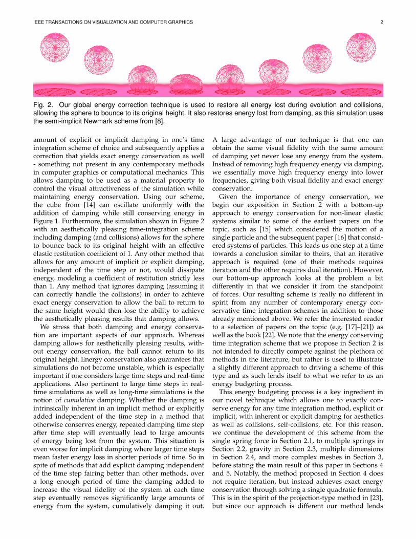
Fig. 8. A single tetrahedron with edge and altitude springsis stretched and then released. It is evolved using our newspring force, which allows it to oscillate back and forthcontinuously about its rest state. The time step size ofthis simulation is set equal to the framerate.

just triangle altitude springs, as the extension to tetra-hedra is straightforward. An altitude spring is placedbetween each particle of the triangle, and a virtual nodeprojected onto the plane of the opposite edge. An equaland opposite spring force is applied to the particle andthe virtual node, and the virtual node distributes itsforces barycentrically to the particles of the edge. Asdiscussed in [26], the inverse mass and velocity of thisvirtual node are defined as

1

mv=

„w2

1

m1+

w22

m2

«(36)

vv = w1v1 + w2v2 (37)

where nodes 1 and 2 form the edge along which thevirtual node lies, and w1 and w2 are the barycentricweights of those two nodes. If one considers a singlealtitude spring in isolation where the altitude goes fromnode 3 to the edge formed by nodes 1 and 2, then theequation for ∆KE becomes

∆KE =1

2mv

h(vn+1

v )T(vn+1v ) − (vn

v)T(vnv)

i+

1

2m2

h(vn+1

3 )T(vn+13 ) − (vn

3 )T(vn3 )

i(38)

=1

2∆t2

„1

mv+

1

m3

«F 2 + ∆t((vn

v)Tu− (vn3 )Tu)F (39)

which we note is exactly what one gets with a normalspring, except that one of the endpoints is replacedby the weighted sum of two nodes. The equation for∆PE is easily modified in a similar fashion. However,as noted in [27], if all three altitude springs in a tri-angle are used at once, one might encounter negativebarycentric weights. To prevent these degenerate cases,we only ever use the shortest altitude spring, which alsomeans we only need to keep track of one PEres pertriangle/tetrahedron. However, as the shortest altitudespring will switch throughout the course of a simulation,and because the restlength and Young’s modulus maybe different for each altitude, simply switching springswhile using the same PEres is not sufficient. To handle

Fig. 9. A graph showing the total energy at the endof each frame in the simulation of a single tetrahedronwith altitude springs shown in Figure 8. The green lineshows the energy using our new energy conservingspring forces, and the red line shows the total energy ifnormal spring forces were used for that frame.


Fig. 10. Two connected triangles with edge, altitude,and bending springs are constrained at their non-sharednodes. The shared nodes are given an initial velocity,and the triangles are evolved using our new spring force,allowing the triangles to oscillate back and forth abouttheir rest state. The time step size of this simulation isset equal to the framerate.

this, whenever we switch altitude springs in a triangleor tetrahedra, we update the PEres associated with thatelement as follows

I. PEtotal = PEold altitude − PEres

II. PEres = PEnew altitude − PEtotal

This ensures that energy is conserved when altitudesprings are added and removed from the simulation. Asfuture work, it would be interesting to try to adapt thisscheme to a method that handles remeshing, such as [28].Figure 10 shows a simulation with energy conservingtriangle altitude springs, and Figure 8 shows the exten-sion of this method to energy conserving tetrahedronaltitude springs. Figure 9 shows the total energy at theend of each frame in the simulation, where the greenline shows the energy using our new energy conservingspring forces, and the red line shows the total energy ifnormal spring forces were used for that frame.

3.2 Bending Springs

To simulate thin deformable materials such as cloth, weadd a simple bending model composed of two springsto resist bending motion. One of these springs connectsopposite vertices across an edge shared by two trianglesand can be made energy conserving by simply consid-ering what is done for normal edge springs, as it justconnects two nodes in the mesh. However, if the twotriangles become coplanar, this spring cannot recover therest curvature as it lies in-plane with the triangles. Asecond axial bending spring is added to alleviate thisproblem by connecting a virtual node on the shared edgeto a virtual node on the first bending spring.

To make the axial bending spring energy conserv-ing, we apply a similar approach to handling altitudesprings, except that instead of only one endpoint beinga virtual node, both endpoints are now virtual nodes.However, one will notice that this axial bending springis actually a zero-length spring. To handle this in ourenergy conserving framework, we first recall that thepotential energy of a zero-length spring is

PEzero−length =1

2

k

l0(l − l0)2 (40)

where the only difference with a normal spring is theuse of the visual restlength l0 in addition to the normalrestlength l0, which prevents division by zero. Replacing

l0 by l0 in equation 4 allows us to handle zero-lengthsprings in an energy conserving way. Figure 10 showsa simple example of these energy conserving bendingsprings. It is feasible that these ideas could be extendedto other bending models, such as [8], [29], [30]. Moreover,we imagine one could extend these energy conservationtechniques to other models based on mass-spring sys-tems, such as the hard and soft constraints in [26] (seealso [31]).

4 OUR NEW SCHEME

In Section 2 we outlined a force based iterative approachto conserving energy in a mass-spring system whichrelied on an energy budgeting process where exactchanges in kinetic and potential energy were computedand the net change in energy was denoted PEres =∆KE+∆PE. Using an iterative approach one can drivePEres to zero, which is the typical goal of contemporaryenergy conserving time integration schemes. However,we instead exploited the ability to carry non-zero val-ues of PEres forward in order to simplify the iterativeschemes in multiple dimensions in Section 2.4 and inorder to cut down on the number of iterations required.In this section we propose our novel approach to energyconservation which allows one to set PEres to zeroexactly conserving energy by solving a simple quadraticequation requiring no iteration. In fact one could usetheir favorite time integration scheme with their favoriteforces, including elasticity and damping(!), and simplyinsert their value of F into the formulas for ∆KE and∆PE in order to compute PEres for their scheme. Thenour new global correction method (explained below)would allow them to exactly conserve the energy in postprocess for that scheme. Because one only needs to knowPEres for their favorite scheme, we dedicated Section 3to a few more complex elements such as altitude andbending springs to give the reader some insight into howthey might compute PEres for various elements.

4.1 MotivationFirst, for the sake of motivation, let us consider etherdrag, which usually takes the velocity and scales it backbased on some ether drag coefficient. Now, imagine if amesh had too much energy as indicated by PEres. Onecould simply add some ether drag to every node to sloweverything down, such that the overall change in kineticenergy due to ether drag accounts for the total PEresstill present in the mesh. We write this down as

KEafter − KEbefore = −X

PEres (41)X 1

2m

h(vn+1)Tvn+1 − (vn)Tvn

i= −

XPEres (42)

where

vn+1 = vn −∆t

mεvn (43)

This simplifies toX∆t

»−ε +

1

2

∆t

mε2

–(vn)Tvn = −

XPEres (44)


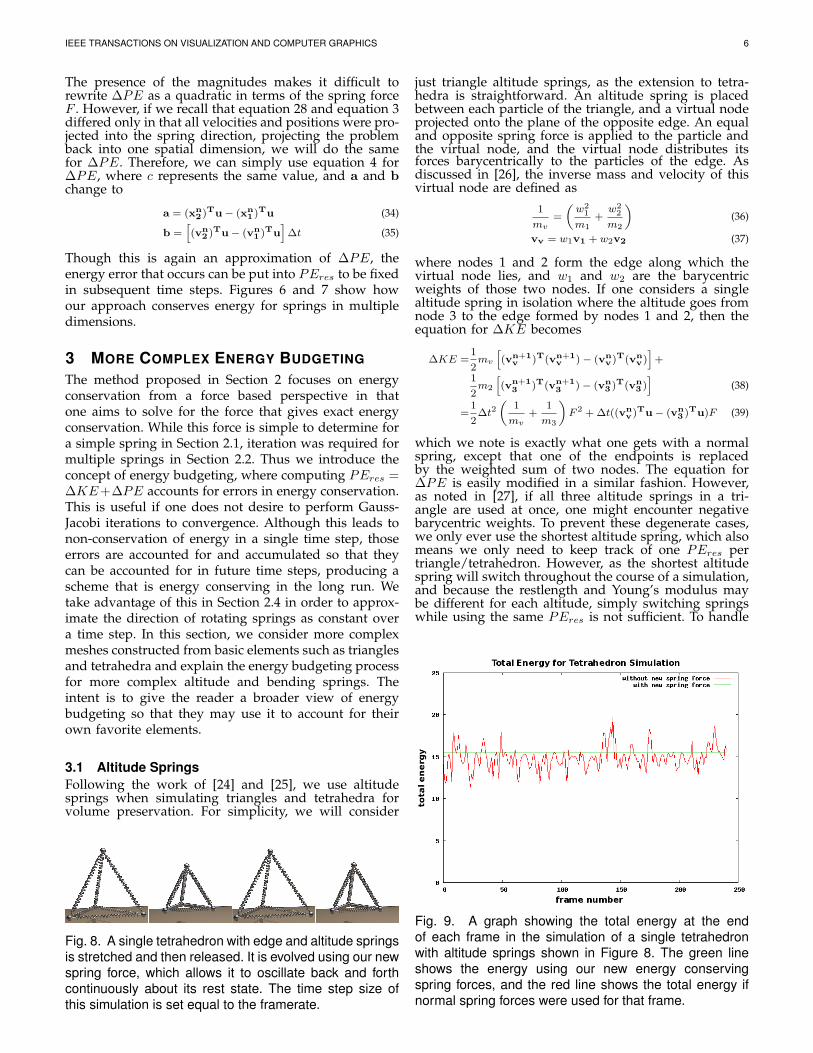
Fig. 11. A piece of cloth is constrained by two pointsand let go from its horizontal initial state. Our energyconservation framework enables it to continue swingingback and forth and achieve its initial height.

where ε is the global ether drag coefficient. Thisquadratic equation can be solved for ε, which producesan ether drag force on each node that will decrease theglobal energy to be closer to the correct amount. Ofcourse one can only decrease the KE to zero, so therecould still be PEres left over to be fixed in the nexttime step, but applying this global correction will bringthe total energy closer to the correct amount. If insteadthe mesh did not have enough energy, one could dothe opposite of ether drag and increase all the velocitiesslightly to get the correct total energy.

Since ether drag does not conserve momentum we donot propose using it as a method to fix the global energy,but it is useful in conceptualizing the main idea. We willnow introduce two momentum preserving forces thatcan be used in a similar way to correct the total energywhile also conserving momentum.

4.2 Momentum Conserving Correction ForcesThe motivational exposition in Section 4.1 for etherdrag actually extends in a straightforward way to otherforces that conserve momentum. The first force we willconsider is the elastic spring force used in the standardvelocity update. Replacing the elastic force for the etherdrag force in equation 42 givesX 1

2m

h(vn+1)Tvn+1 − (vn)Tvn

i= −

XPEres (45)

where

vn+1 = vn −∆t

mε

XFe (46)

This simplifies toX∆t

»−ε(vn)T

XFe +

∆t

2mε2

XFT

e

XFe

–= −

XPEres

(47)

where∑

Fe is the sum of all elastic forces felt on aspecific node. Again, we have a quadratic in ε, which wecan solve in the same manner as when using ether drag.Using the elastic force instead of an ether drag forceallows the global energy correction to be momentumconserving.

Instead of using the elastic force for the global cor-rection, one could also use the damping force from the

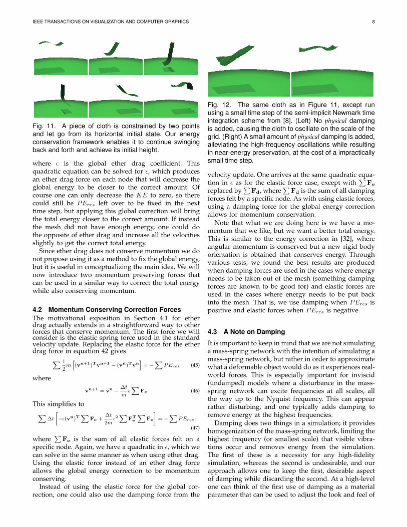
Fig. 12. The same cloth as in Figure 11, except runusing a small time step of the semi-implicit Newmark timeintegration scheme from [8]. (Left) No physical dampingis added, causing the cloth to oscillate on the scale of thegrid. (Right) A small amount of physical damping is added,alleviating the high-frequency oscillations while resultingin near-energy preservation, at the cost of a impracticallysmall time step.

velocity update. One arrives at the same quadratic equa-tion in ε as for the elastic force case, except with

∑Fe

replaced by∑

Fd, where∑

Fd is the sum of all dampingforces felt by a specific node. As with using elastic forces,using a damping force for the global energy correctionallows for momentum conservation.

Note that what we are doing here is we have a mo-mentum that we like, but we want a better total energy.This is similar to the energy correction in [32], whereangular momentum is conserved but a new rigid bodyorientation is obtained that conserves energy. Throughvarious tests, we found the best results are producedwhen damping forces are used in the cases where energyneeds to be taken out of the mesh (something dampingforces are known to be good for) and elastic forces areused in the cases where energy needs to be put backinto the mesh. That is, we use damping when PEres ispositive and elastic forces when PEres is negative.

4.3 A Note on Damping

It is important to keep in mind that we are not simulatinga mass-spring network with the intention of simulating amass-spring network, but rather in order to approximatewhat a deformable object would do as it experiences real-world forces. This is especially important for inviscid(undamped) models where a disturbance in the mass-spring network can excite frequencies at all scales, allthe way up to the Nyquist frequency. This can appearrather disturbing, and one typically adds damping toremove energy at the highest frequencies.

Damping does two things in a simulation; it provideshomogenization of the mass-spring network, limiting thehighest frequency (or smallest scale) that visible vibra-tions occur and removes energy from the simulation.The first of these is a necessity for any high-fidelitysimulation, whereas the second is undesirable, and ourapproach allows one to keep the first, desirable aspectof damping while discarding the second. At a high-levelone can think of the first use of damping as a materialparameter that can be used to adjust the look and feel of


a simulation, whereas the second use is strictly to removeenergy.

Furthermore it is important to note that for a givensimulation on a given mesh, damping can be minimizedbut not removed entirely. Take Figure 11, where we showthat a highly deformable piece of cloth is able to recoverits initial height when using our energy conservationframework. We reran it using a very small time stepof the semi-implicit Newmark integration scheme of [8],which made the simulation take quite a long time to run.A time step this small could never be used in practicebut we did it to minimize numerical dissipation as muchas possible. Then to minimize physical dissipation we setthe damping to zero; Figure 12 (Left) shows the result.The cloth mesh starts to oscillate on the scale of the grid- as we pointed out earlier in Section 1, this is similarto what is achieved by a variational method withoutdamping. Energy is preserved but the simulation doesnot mimic an expected material behavior but rathershows frequencies particular to the scale of the mesh.If we add just a very small amount of physical damping,increasing it to .0001, we get the result in Figure 12(Right), with rather nice energy preserving behavior.This is about the best we can do preserving energy inthis example, using an impractically small time step anda hand-tuned, very small amount of damping. Now fora different mesh, simulation example, time integrationscheme, and mass-spring model one might do better,but the issues are symptomatic. Numerical damping canbe driven very low with impractically small time steps,and physical damping can be set very low but stillneeds to be big enough to “hide” the mesh discretization.This is the same conclusion that those doing variationalmethods come to without having stated it. One can thinkof our method in some ways as a better constitutivemodel for the mesh - one that does a better job modelinga real material without discretization artifacts while notrequiring the removal of energy from the system (eitherwith numerical or with physical damping).

4.4 Correcting Arbitrary Time IntegratorsIn summary, the key idea of our method is to compute aPEres and then apply the correction forces in Section 4.2to obtain energy conservation. Those correction forces

Fig. 13. A complex deformable armadillo is stretched andreleased with its feet constrained. Our energy conserva-tion framework allows the armadillo to maintain its energyand continue bouncing over time.

can be used on any mesh, whether it be discretized withmasses and springs or even finite elements. Whereasthe correction forces are proposed in a mass-springformulation, the original forces used in the simulationcould come from a finite element model as long asPEres is properly computed. In fact one could use a timeintegration scheme of their choice, whether it be implicit,semi-implicit, explicit, variational, symplectic, geometric,etc., and as long as PEres can be computed via anenergy budgeting process, one can use the correctionforces in Section 4.2 to achieve energy conservation.Moreover, the original time integration method can in-clude both elastic and damping forces, with dampingbeing especially important because it gives aestheticappeal to a simulation. In fact we chose the methodfrom [8] with visually appealing damping parametersfor Figures 2, 11, 13, 15, and 16. In each simulation,we simply computed PEres in each time step using themethods outlined in Sections 2 and 3 and subsequentlycalculated correction forces along the lines of Section 4.2.

In Figure 14, the red line shows the results usingthe standard scheme from [8] to simulate the bouncingsphere shown in Figure 2. However, using our energybudgeting process to compute PEres and then apply ourcorrection forces leads to the green graph, where energyis obviously much better conserved. Note that while thefact that one can only decrease the KE to zero indicatesthat one cannot always exactly zero out PEres every timestep with the correction forces, any left over PEres ineach time step accumulates and is fixed in future timesteps. As can be seen by comparing the green and redlines on the graph, the correction makes an enormous

Fig. 14. A graph showing the total energy over time in thesimulation of the coarse tetrahedralized sphere shown inFigure 2. The red line is the total energy when our energyconservation scheme is not used, whereas the green lineis the total energy when utilizing our new scheme. Thesudden declines in the red line correspond to collisionsbetween the sphere and the ground.


Fig. 15. A deformable wheel is dropped from a height and collides with the ground and itself, producing bothrigid/deformable and self-collisions. Our global energy correction technique is used to restore all energy lost duringevolution and collisions, allowing the wheel to bounce to its original height.

difference in the simulation and produces a line thatappears constant to the naked eye.

5 COLLISIONSAn obvious benefit of our energy budgeting process isthat we can readily incorporate both collisions and self-collisions. Collisions are handled using the integrationscheme

I. vn+1/2 = vn + ∆t2m

F

II. xn+1 = xn + ∆tvn+1/2

III. Collisions: Modify vn and xn+1

IV. Self-Collisions: Modify vn and xn+1

V. vn+1 = vn + ∆tm

F (collision constraints in CG solve)

First, let us consider what happens during collisionswith rigid bodies. In step III above, when a particlecollides with a rigid body, its velocity is set to thevelocity of the body, resulting in a change in kineticenergy. Moreover, the particle is moved to the surfaceof the body, resulting in a change in potential energyfor all springs attached to that particle. If energy is to beconserved, the ∆KE due to collisions must equal −∆PEdue to collisions. Typically, energy is not conserved dur-ing collisions and often increases. We stress that stifferobjects and larger time steps result in a more drastic∆PE due to collisions. As a result, large energy errorswill be made, which could potentially result in unstablesimulations. To ensure energy is conserved throughoutthe simulation, we compute the energy error ∆KE +∆PE due to collisions, and use our global correctionfrom Section 4 to correct it. Even if one does not intendto use our algorithm for energy conservation at all,monitoring the energy difference during collisions andidentifying any time steps where the energy increaseswould be important.

As in [6], [26], [33], we use collisions as constraints onvn+1 in the conjugate gradients solve during the velocityupdate in step V above. In this case, we would againlike to determine the ∆KE due to using these collisionconstraints, as this will allow us to determine the energygained or lost due to this part of collisions. However,as these constraints are enforced as projections in thesolve, which includes elastic and damping forces as well,one cannot simply measure the kinetic energy beforeand after the solve. In order to determine the ∆KEdue to just the collision constraints, we take the ∆KEcomputed after the CG solve, and subtract off the ∆KEthat would have resulted by applying just the elasticand the damping forces. Once this is determined, any

energy gained or lost can be corrected using the globalcorrection from Section 4.

Figure 2 shows an example of an energy conservingsimulation including collisions. We note our methodmakes it possible to restore only part of the energy lostto collisions, allowing an animator to explicitly controlhow much energy collisions remove from the simulation.It is important to note that similar energy conservationapproaches can be applied to other collision handlingschemes. For more on collision handling techniques, werefer the interested reader to the recent paper of [34].

5.1 Self-Collisions

As the amount of deformation in a mesh becomesmore significant, it becomes important to handle self-collisions, which we handle using the method of [7].We first note that self-collisions change both positionsand velocities, resulting in changes to both PE and KE.Moreover, no energy should be lost to self-collisions, asall forces are exchanged between elements of the mesh.Therefore, to conserve energy, we simply measure boththe kinetic and potential energy before and after self-collisions are applied and fix any error ∆KE + ∆PEwith the global correction described in Section 4. InFigure 15, we show an energy conserving simulationwith self collisions.

We note that there are many other techniques forhandling self-collisions, referring the interested readerto [35], and stress that similar energy conservation tech-niques could be applied to these other methods. Inparticular, [36] showed that under various situations,such as when cloth is pinched in the armpit of a character(between two bodies), it is sometimes desirable to allowinterpenetration of cloth, which can be untangled after-wards. Note that this untangling requires changing ofboth positions and velocities of the cloth mesh, leading tochanges in potential and kinetic energy. If these changesare undesired, they can be accounted for and correctedwith our global correction method.

6 EXAMPLES

In Figure 2, we show a deformable sphere bouncing onthe ground, and by using our global energy correctionframework, it is able to recover its initial height whilemaintaining interesting oscillations due to the collision


Fig. 16. A complex deformable armadillo model is dropped down a flight of stairs, exhibiting both rigid/deformable andself-collisions.

with the ground. We show that the same global en-ergy correction can be applied to simulations with self-collisions in Figure 15, where we drop a deformablewheel on the ground. Even with both rigid/deformableand self-collisions, the wheel is able to regain its ini-tial height. In Figure 11, we show that a highly de-formable piece of cloth also is able to recover its initialheight when using our energy conservation framework.It would be interesting to see if we could extend ourmethods, especially the energy conserving global fix inSection 4, to consider other models for cloth, such as theyarn based model seen in [37]. In the attached videos, aslight artifact is apparent in the bouncing sphere videoswhen the stiffness is high, causing the sphere to bounceoff-center. We hypothesize that this is due to the dis-cretization of the sphere, as it is noticeably worse whena coarse discretization is used, and when the sphere isnot allowed to deform significantly, allowing the initialpoint of impact to play a significant role in determiningthe direction of the sphere’s bounce. A similar artifact isseen in the video of the hanging cloth, where the swingof the cloth changes towards the end of the video. Weagain believe this bias is due to the coarseness of the dis-cretization, with the cloth containing roughly only 5500triangles. It would be interesting to see if increasing theresolution of the meshes and improving the symmetryof the discretization removes these simulation artifacts.

Finally, we show that our energy conservation frame-work works on complex meshes as well. In Figure 13, westretch a complex armadillo mesh out and, while con-straining its feet, we release it and let it bounce around.Using a typical deformable mesh solver, one would seethis motion damp out over time; using our frameworkthe armadillo continues to move around while conserv-ing energy. In Figure 16, we drop the armadillo downa flight of stairs, showing that rigid/deformable colli-sions and self-collisions continue to work with complexmeshes.

Energy budgeting, i.e. calculating PEres, is rather

straightforward and adds very little overhead to the costof the simulation. Similarly, the calculation of the cor-rection forces is also straightforward and approximatelyequivalent to one explicit time step. Overall in oursimulations, the simulation time was dominated by theconjugate gradient solve to implicitly handle viscosityand our energy budgeting correction forces were similarin cost to the explicit part of the time step.

7 CONCLUSION

We introduced a novel technique for energy conserv-ing simulation of deformable bodies regardless of theunderlying time integration scheme. Our scheme allowsthe incorporation of collisions, self-collisions, and mostimportantly damping, which, as authors of other energyconserving integration schemes have pointed out, iscrucial to the aesthetics of a simulation. However, unlikeother energy conserving schemes where the additionof visually appealing damping necessarily removes theenergy conservation property, our approach allows oneto maintain energy conservation while using dampingas a material parameter to improve the aesthetics of thesimulation. Finally, the energy budgeting approach thatour method takes allows it to be applied as a lightweightpost-process energy fix to the time integration methodof one’s choice, allowing one to conserve as much or aslittle energy as is visually desirable.

One of the main limitations with the global correctionscheme we proposed is that it does not provide controlover where in the mesh the energy error is distributed. Infuture work, we would like to explore different momen-tum conserving correction forces similar to those pre-sented in Section 4.2, but which allow the energy error tobe distributed less uniformly or targeted to specific partsof the mesh. Furthermore, we are interested in exploringwhether other less simplistic forces could be used withour global correction, and whether these forces producemore visually appealing results as compared to simplyscaling the damping or elastic forces.


In Figures 2, 15, and 16, we show how our globalenergy correction works in the presence of collisionswith kinematic objects. In future work, we would liketo explore how our global energy correction extends tothe interaction of multiple dynamic objects. Namely, onecould keep track of the energy error due only to thecollision of two bodies, and distribute that error back tothe two bodies by applying an epsilon-scaled version ofthe original collision forces, much like the other globalcorrection schemes we introduced in Sections 4 and 5.This will ensure that energy is conserved during multi-ple object interaction, while maintaining conservation ofmomentum.

Finally, we have only experimentally tested our globalcorrection for a mass-spring based system using a semi-implicit Newmark integration scheme. Nothing in ourglobal correction scheme is specific to mass-spring sys-tems or semi-implicit Newmark integration, and in fu-ture work we would like to explore the generality of ourcorrection scheme in the context of other solvers.

ACKNOWLEDGEMENTS

The authors would like to acknowledge Craig Schroederfor his help with rendering. Research supported in partby NSF IIS-1048573, ONR N00014-09-1-0101, ARL AH-PCRC W911NF-07-0027 and the Intel Science and Tech-nology Center for Visual Computing. J.S. was supportedin part by an NSF Graduate Research Fellowship.

REFERENCES

[1] D. Terzopoulos, J. Platt, A. Barr, and K. Fleischer, “Elastically de-formable models,” Comput. Graph. (Proc. SIGGRAPH 87), vol. 21,no. 4, pp. 205–214, 1987.

[2] D. Terzopoulos and K. Fleischer, “Deformable models,” The Vis.Comput., vol. 4, no. 6, pp. 306–331, 1988.

[3] ——, “Modeling inelastic deformation: viscoelasticity, plasticity,fracture,” Comput. Graph. (SIGGRAPH Proc.), pp. 269–278, 1988.

[4] J. O’Brien and J. Hodgins, “Graphical modeling and animation ofbrittle fracture,” in Proc. of SIGGRAPH 1999, 1999, pp. 137–146.

[5] G. Irving, J. Teran, and R. Fedkiw, “Invertible finite elementsfor robust simulation of large deformation,” in Proc. of the ACMSIGGRAPH/Eurographics Symp. on Comput. Anim., 2004, pp. 131–140.

[6] D. Baraff and A. Witkin, “Large steps in cloth simulation,” inACM SIGGRAPH 98. ACM Press/ACM SIGGRAPH, 1998, pp.43–54.

[7] R. Bridson, R. Fedkiw, and J. Anderson, “Robust treatment ofcollisions, contact and friction for cloth animation,” ACM Trans.Graph., vol. 21, no. 3, pp. 594–603, 2002.

[8] R. Bridson, S. Marino, and R. Fedkiw, “Simulation of cloth-ing with folds and wrinkles,” in Proc. of the 2003 ACM SIG-GRAPH/Eurographics Symp. on Comput. Anim., 2003, pp. 28–36.

[9] M. Hauth and O. Etzmuss, “A high performance solver forthe animation of deformable objects using advanced numericalmethods,” in Computer Graphics Forum, vol. 20, 2001, pp. 319–328.

[10] K.-J. Choi and H.-S. Ko, “Stable but responsive cloth,” ACM Trans.Graph. (SIGGRAPH Proc.), vol. 21, pp. 604–611, 2002.

[11] L. Kharevych, W. Yang, Y. Tong, E. Kanso, J. Marsden, P. Schroder,and M. Desbrun, “Geometric variational integrators for com-puter animation,” ACM SIGGRAPH/Eurographics Symp. on Com-put. Anim., pp. 43–51, 2006.

[12] I. Chao, U. Pinkall, P. Sanan, and P. Schroder, “A simple geometricmodel for elastic deformations,” in Proc. of ACM SIGGRAPH 2010,2010, pp. 38:1–38:6.

[13] P. Mullen, K. Crane, D. Pavlov, Y. Tong, and M. Desbrun, “Energy-preserving integrators for fluid animation,” in SIGGRAPH ’09:ACM SIGGRAPH 2009 papers, 2009, pp. 1–8.

[14] I. Chao, U. Pinkall, P. Sanan, and P. Schroder, “A simplegeometric model for elastic deformations,” SupplementalMaterials Video, Proc. of ACM SIGGRAPH 2010. [Online].Available: http://dl.acm.org/citation.cfm?id=1778775

[15] R. A. LaBudde and D. Greenspan, “Energy and momentum con-serving methods of arbitrary order for the numerical integrationof equations of motion i. motion of a single particle,” Numer.Math., vol. 25, pp. 323–346, 1976.

[16] ——, “Energy and momentum conserving methods of arbitraryorder for the numerical integration of equations of motion i.motion of a system of particles,” Numer. Math., vol. 26, pp. 1–16, 1976.

[17] C. Kane, J. E. Marsden, M. Ortiz, and M. West, “Variationalintegrators and the newmark algorithm for conservative anddissipative mechanical systems,” International Journal for NumericalMethods in Engineering, vol. 49, pp. 1295–1325, 2000.

[18] A. Lew, J. E. Marsden, M. Ortiz, and M. West, “Variationaltime integrators,” International Journal for Numerical Methods inEngineering, vol. 60, pp. 152–212, 2004.

[19] W. Fong, E. Darve, and A. Lew, “Stability of asynchronousvariational integrators,” J. Comput. Phys., vol. 227, pp. 8367–94,2008.

[20] D. Harmon, E. Vouga, B. Smith, R. Tamstorf, and E. Grinspun,“Asynchronous contact mechanics,” in ACM SIGGRAPH 2009.ACM Press/ACM SIGGRAPH, 2009, pp. 1–12.

[21] M. Gonzalez, B. Schmidt, and M. Ortiz, “Force-stepping integra-tors in lagrangian mechanics,” International Journal for NumericalMethods in Engineering, vol. 84, pp. 1407–1450, 2010.

[22] E. Hairer, G. Wanner, and C. Lubich, Geometric Numerical In-tegration: Structure-Preserving Algorithms for Ordinary DifferentialEquations. Springer Series in Computational Mathematics, 2006,vol. 31.

[23] J. C. Simo, N. Tarnow, and K. K. Wong, “Exact energy-momentumconserving algorithms and symplectic schemes for nonlinear dy-namics,” Comput. Methods Appl. Mech. Eng., vol. 100, pp. 63–116,October 1992.

[24] N. Molino, R. Bridson, J. Teran, and R. Fedkiw, “A crystalline,red green strategy for meshing highly deformable objects withtetrahedra,” in 12th Int. Meshing Roundtable, 2003, pp. 103–114.

[25] R. Bridson, J. Teran, N. Molino, and R. Fedkiw, “Adaptive physicsbased tetrahedral mesh generation using level sets,” Eng. w.Comp., 2005.

[26] E. Sifakis, T. Shinar, G. Irving, and R. Fedkiw, “Hybrid simulationof deformable solids,” in Proc. of ACM SIGGRAPH/EurographicsSymp. on Comput. Anim., 2007, pp. 81–90.

[27] A. Selle, M. Lentine, and R. Fedkiw, “A mass spring model forhair simulation,” ACM Transactions on Graphics, vol. 27, no. 3, pp.64.1–64.11, Aug. 2008.

[28] M. Wicke, D. Ritchie, B. Klingner, S. Burke, J. Shewchuk, andO’Brien, “Dynamic local remeshing for elastoplastic simulation,”in Proc. of ACM SIGGRAPH 2010, 2010, pp. 49:1–49:11.

[29] E. Grinspun, A. Hirani, M. Desbrun, and P. Schroder, “Discreteshells,” in Proc. of the 2003 ACM SIGGRAPH/Eurographics Symp.on Comput. Anim., 2003, pp. 62–67.

[30] P. Volino and N. Magnenat-Thalmann, “Simple linear bend-ing stiffness in particle systems,” in Proc. of the ACM SIG-GRAPH/Eurographics Symp. on Comput. Anim., 2006, pp. 101–105.

[31] C. Twigg and Z. Kacic-Alesic, “Point cloud glue: Constrainingsimulations using the procrustes transform,” in Proc. of the 2010ACM SIGGRAPH/Eurographics Symp. on Comput. Anim., 2010, pp.45–54.

[32] J. Su, C. Schroeder, and R. Fedkiw, “Energy stability and fracturefor frame rate rigid body simulations,” in Proceedings of the 2009ACM SIGGRAPH/Eurographics Symp. on Comput. Anim., 2009, pp.155–164.

[33] T. Shinar, C. Schroeder, and R. Fedkiw, “Two-way coupling ofrigid and deformable bodies,” in SCA ’08: Proceedings of the 2008ACM SIGGRAPH/Eurographics symposium on Computer animation,2008, pp. 95–103.

[34] J. Allard, F. Faure, H. Courtecuisse, F. Falipou, C. Duriez, andP. Kry, “Volume contact constraints at arbitrary resolution,” inProc. of ACM SIGGRAPH 2010, 2010, pp. 82:1–82:10.

[35] J. Barbic and D. James, “Subspace self-collision culling,” in Proc.of ACM SIGGRAPH 2010, 2010, pp. 81:1–81:9.


[36] D. Baraff, A. Witkin, and M. Kass, “Untangling cloth,” ACM Trans.Graph. (SIGGRAPH Proc.), vol. 22, pp. 862–870, 2003.

[37] J. Kaldor, D. James, and S. Marschner, “Efficient yarn-based clothwith adaptive contact linearization,” in Proc. of ACM SIGGRAPH2010, 2010, pp. 105:1–105:10.

Jonathan Su received his Ph.D. in ComputerScience from Stanford University in 2011, duringwhich he was awarded the National ScienceFoundation Graduate Research Fellowship. Heis currently a Research Scientist in the ParallelComputing Lab at Intel Corporation where hehas been studying the scalability of physical sim-ulation algorithms on current and future multi-core/many-core architectures.

Rahul Sheth received his B.S.E. in Electricaland Computer Engineering from Rutgers Univer-sity in 2010. While there, he worked on variousresearch projects in visualization and computervision. He is currently pursuing a Ph.D. in Com-puter Science at Stanford University and is in-terested in developing algorithms for real-timephysical simulation.

Ron Fedkiw received his Ph.D. in Mathemat-ics from UCLA in 1996 and did postdoctoralstudies both at UCLA in Mathematics and atCaltech in Aeronautics before joining the Stan-ford Computer Science Department. He wasawarded an Academy Award from The Academyof Motion Picture Arts and Sciences, the Na-tional Academy of Science Award for Initiativesin Research, a Packard Foundation Fellowship,a Presidential Early Career Award for Scientistsand Engineers (PECASE), a Sloan Research

Fellowship, the ACM Siggraph Significant New Researcher Award, anOffice of Naval Research Young Investigator Program Award (ONRYIP), the Okawa Foundation Research Grant, the Robert Bosch FacultyScholarship, the Robert N. Noyce Family Faculty Scholarship, two dis-tinguished teaching awards, etc. Currently he is on the editorial board ofthe Journal of Computational Physics, Journal of Scientific Computing,and he participates in the reviewing process of a number of journalsand funding agencies. He has published over 80 research papers incomputational physics, computer graphics and vision, as well as a bookon level set methods. For the past ten years, he has been a consultantwith Industrial Light + Magic. He received screen credits for his work on“Terminator 3: Rise of the Machines”, “Star Wars: Episode III - Revengeof the Sith”, “Poseidon” and “Evan Almighty”.

Documents

IEEE TRANSACTIONS ON VISUALIZATION AND COMPUTER GRAPHICS 1 Energy