Embed Size (px)
Citation preview

IEEE TRANSACTIONS ON VISUALIZATION AND COMPUTER GRAPHICS, MANUSCRIPT ID 1
Scalable Analysis of Movement Data for Extracting and Exploring Significant Places
Gennady Andrienko, Natalia Andrienko, Christophe Hurter, Salvatore Rinzivillo, Stefan Wrobel
Abstract— Place-oriented analysis of movement data, i.e., recorded tracks of moving objects, includes finding places of interest in which certain types of movement events occur repeatedly and investigating the temporal distribution of event occurrences in these places and, possibly, other characteristics of the places and links between them. For this class of problems, we propose a visual analytics procedure consisting of four major steps: (1) event extraction from trajectories; (2) extraction of relevant places based on event clustering; (3) spatio-temporal aggregation of events or trajectories; (4) analysis of the aggregated data. All steps can be fulfilled in a scalable way with respect to the amount of the data under analysis; therefore, the procedure is not limited by the size of the computer’s RAM and can be applied to very large datasets. We demonstrate the use of the procedure by example of two real-world problems requiring analysis at different spatial scales.
Keywords — movement, trajectories, spatio-temporal data, spatial events, spatial clustering, spatio-temporal clustering
—————————— ——————————
1 INTRODUCTIONovement data describing changes of spatial positions of discrete mobile objects are nowadays collected in huge amounts by means of current tracking technologies, such as
GPS, RFID, radars, and others. Automatically collected movement data are semantically poor as they basically consist of object identi-fiers, coordinates in space, and time stamps. Despite that, valuable information about the objects and their movement behavior as well as about the space and time in which they move can be gained from movement data by means of analysis [2].
Movement can be viewed as consisting of continuous paths in space and time [23], also called trajectories, or as a composition of various spatial events [4]. As noted in [10] and [37], there are many definitions of the term event. We adhere to Kim’s definition of events as exemplifications of properties or relationships at some times [28]. Spatial events are events localized in space [10].
The event-based view of movement is particularly suitable for applications and tasks where analysts are interested in occurrences of certain movement characteristics such as very high or very low speeds, high acceleration, sharp turn, etc., or certain kinds of rela-tionships between the moving objects and other objects around them, such as encountering or moving close to each other. An occurrence of the movement characteristic or relationship of inter-est is a spatial event. Such events will be further called movement events, or m-events.
There is a class of problems where analysts need to find places in which m-events of a certain type occur repeatedly and then do further analysis related to these places. For example, having tracks of multiple cars in a city, a traffic analyst may first need to find places where traffic jams occur and then investigate in which times of the day they happen and how long they last. From trails of mi-gratory birds, an ornithologist may wish to extract places where the birds stop for resting and feeding and then analyze the temporal patterns of visiting these places and travelling between the places. We point out that relevant places can only be delineated by pro-
cessing movement data, that is, there is no predefined set of places (e.g., compartments of a territory division) from which the analyst can select places of interest. The relevant places may have arbitrary shapes and sizes and irregular spatial distribution. They may even overlap in space; hence, approaches based on dividing the territory into non-overlapping areas (as in [5]) are not appropriate.
We propose a visual analytics procedure for place-oriented anal-ysis of movement data that includes (1) visually-supported extrac-tion of relevant m-events, (2) finding and delineating significant places on the basis of clustering of the m-events according to dif-ferent attributes, (3) spatio-temporal aggregation of the m-events and movement data by the defined places or pairs of places and time intervals; (4) analysis of the aggregated data for studying the spatio-temporal patterns of event occurrences and/or connections between the places. In comparison to the previous work [3], we have developed a scalable version of the procedure. It can be ap-plied to large datasets that cannot be fully loaded in RAM for processing and analysis. We would like to stress the generic char-acter of the procedure. It is not oriented to any particular applica-tion domain, but it addresses a class of problems that may arise in various domains. We also stress that the paper is not meant to describe any particular software implementation of the procedure. It only shows some possibilities, mainly for illustrative purposes.
In the following, we first introduce the concepts needed for talk-ing about movement data (section 2) and give an overview of related research (section 3). To make the suggested procedure easier to understand, we first introduce it by an example (section 4) and then present in a more general way (section 5). In section 6, we describe how the procedure is applied to very large data not fitting in RAM. Before concluding the paper, we give one more example where the procedure is applied to a different kind of movement and on a different spatial scale.
2 MOVEMENT DATA AND POSSIBLE DERIVATIVES Movement data consist of position records <object identifier, time, spatial coordinates>. Temporally ordered position records of one object represent the trajectory of this object. The real trajectory is continuous (i.e., the object has some position at any time moment) while the data representing it are discrete (i.e., positions are speci-fied for a sample of time moments). When the time intervals be-tween the known positions are sufficiently short, the intermediate positions can be estimated by means of linear or non-linear interpo-
xxxx-xxxx/0x/$xx.00 © 200x IEEE
———————————————— Gennady Andrienko, Natalia Andrienko and Stefan Wrobel are with
Fraunhofer IAIS (Intelligent Analysis and Information Systems), Sankt Augustin, and University of Bonn, Germany. E-mail: [email protected].
Christophe Hurter is with DGAC/DTI R&D, ENAC and the University of Toulouse, France
Salvatore Rinzivillo is with KDDLab, ISTI – CNR, Pisa, Italy
Manuscript received 15 February 2012
M
Digital Object Indentifier 10.1109/TVCG.2012.311 1077-2626/12/$26.00 © 2012 IEEE
This article has been accepted for publication in a future issue of this journal, but has not been fully edited. Content may change prior to final publication.

2 IEEE TRANSACTIONS ON VISUALIZATION AND COMPUTER GRAPHICS, MANUSCRIPT ID
lation [32][2]. From reconstructed trajectories, one can compute a number of
instant, interval, and cumulative characteristics of the movement. Instant movement characteristics include instant speed, direction, acceleration (change of speed), and turn (change of direction) [21]. Interval characteristics are computed for time intervals of a chosen constant length before, after, or around a given time moment. They include traveled distance, displacement, average speed, sinuosity, tortuousity, as well as statistics of the instant characteristics. Cumu-lative characteristics are computed for the interval from the start of the trajectory to a given time moment or for the remaining interval to the end of the trajectory. Cumulative measures include all inter-val measures and the temporal distances to the starts and ends of the trajectories.
Movement takes place in spatio-temporal context [4], which in-cludes spatial locations and time units with their specific proper-ties, as well as various spatial, temporal, and spatio-temporal enti-ties existing in the space and/or time. For each point or segment of a moving object’s trajectory, all previous and following movements of this object also belong to the spatio-temporal context.
As an object moves, various spatial, temporal, and spatio-temporal relations occur between this object and elements of the context. Some types of relations, such as topological relations ‘in’, ‘cross’, ‘touch’, are called qualitative [17] and are represented by predicates. Other types of relations, such as spatial and temporal distance and spatial direction, are called metric [31] and are repre-sented by numeric-valued functions. For a selected element or set of elements of the context and a selected relation type, it is possible to compute the value of the respective predicate or function in each time moment of a moving object’s trajectory. This requires availa-bility of data about the spatial and temporal positions of the select-ed context elements. For some context elements, such as other moving objects or previous movements of an object, the positions can be extracted from the set of trajectories. For other context elements, additional data (called context data) need to be provided, for example, coordinates of places of interest or times and locations of events of interest.
Movement characteristics and relations to the context can be rep-resented by dynamic (i.e., time-varying) attributes. Besides the attributes that can be computed from reconstructed trajectories and context data, some dynamic attributes may be originally available in the movement data. By means of queries, one can find points and segments of trajectories having particular values of one or more dynamic attributes. According to the event-based view [4], these are movement events (m-events), which can be extracted from the trajectories into a new dataset and analyzed independently or together with the trajectories.
3 RELATED WORK There is abundant literature concerning analysis of movement, which is currently a hot research topic. Paper [2] gives a summary of major approaches and classes of techniques. Here we consider only the works strongly related to the steps of our procedure. The works are grouped according to these steps.
Extraction of events from movement data. The possibility of extracting spatial events from different types of spatio-temporal data is discussed in [10] but concrete methods are not presented. Moving object databases [21] compute various dynamic attributes (numeric functions and predicates) and provide a powerful query language for extracting parts of trajectories based on these attrib-utes. However, there is no convenient user interface for query specification and for viewing the results. Paper [4] describes a visual query tool that computes and visualizes some of the move-ment characteristics and distances to selected context elements and filters trajectory segments based on values of one or more dynamic attributes. In [15], a graphical user interface is used for specifying queries in terms of instant and interval characteristics, particularly, those that express the geometrical complexity of trajectory seg-
ments (e.g., tortuousity). The tool provides an immediate visual feedback on a map display. In [20], multiple coordinated views and interactive visual queries are used for detecting microscopic traffic patterns and abnormal behaviors on a road crossing; however, filtering is applied to whole trajectories rather than segments.
In [12], relations to the spatio-temporal context are used for computational extraction of m-events from trajectories of mobile phone users. The authors extract sufficiently long stops occurring in spatial and temporal proximity to known public events. They also extract stop events occurring in the night hours in order to determine the home locations of the people. In [38], stop events are extracted from car trajectories based on the speed values; then, additional context information (e.g., points of interest) is used to separate meaningful stops from non-meaningful.
In [30] and [14], instant and interval movement characteristics are used to decompose trajectories into episodes of homogeneous movement, which are then used for detecting particular movement patterns [30] or classification of movement modes [14].
Spatial clustering of events and definition of relevant places. Paper [19] applies density-based spatial clustering to points of multiple trajectories to delineate areas of intense traffic. Then frequent sequences of visited areas with typical transition times (T-patterns) are extracted by means of data mining methods. In [35], a specific kernel density estimation method is applied to trajectories. It allows detecting particular places, e.g., anchoring areas of ships. In [8], a special algorithm for spatially constrained clustering is applied to points extracted from trajectories. It makes clusters of desired spatial extents, which are then used for territory tessella-tion. Density-based clustering of trajectory points over successive time slices is used in [27] for finding moving clusters of objects rather than places of interest.
Aggregation of event and movement data. In [18], spatial, temporal, and categorical (attribute-based) aggregation of traffic events is done using predefined areas of interest. Paper [1] surveys the existing approaches to aggregation of movement data and visual exploration of the aggregates. The data are typically aggre-gated by predefined areas. In [8], a territory is first divided into compartments based on the spatial distribution of characteristic points extracted from trajectories and then the compartments are used for spatio-temporal aggregation of the data. The most usual types of aggregated movement data are time series associated with places or with flows between places. T-patterns extracted in [19] can be viewed as a particular kind of aggregates: the motion dy-namics between places are represented as typical transition times.
Analysis of aggregated movement data. There are many visual and computational methods that can be applied to aggregated movement data. Paper [2] includes a taxonomy of possible ap-proaches, considered on a high abstraction level. Paper [1] surveys specific methods and demonstrates the use of various visualization and interaction techniques. In [36], two-level spatial treemaps are used to study flows among locations. Since aggregated movement data have the form of spatially referenced time series, it is possible to use interactive visualizations [11] and computational methods from statistics [24] and data mining [34] devised for time series.
4 AN EXAMPLE OF PLACE-ORIENTED ANALYSIS In this section, we introduce the suggested visual analytics proce-dure by an illustrated example. Here we only describe what is done. The following sections 5 and 6 will describe in detail how it is done.
The example dataset consists of about 176,000 trajectories (more than 2 million positions in total) of 17,241 cars recorded during one week in April, 2007 on the territory of Milan (Italy) by GPS sen-sors installed in the cars. A sample of the trajectories is shown on a map in fig.1 left.
The analysis problem is to determine the places where traffic congestions occurred and investigate how the traffic situations in these places evolved over the week.
This article has been accepted for publication in a future issue of this journal, but has not been fully edited. Content may change prior to final publication.

ANDRIENKO ET AL.: SCALABLE ANALYSIS OF MOVEMENT DATA FOR EXTRACTING AND EXPLORING SIGNIFICANT PLACES 3
4.1 Extraction of m-events from trajectories An indication of possible traffic congestion in some place is when cars in this place move with low speed. Hence, for detecting con-gestions, we need to extract low speed m-events from the car tra-jectories. Such m-events may be defined as the points of the trajec-tories in which the speed is below a certain threshold.
Choosing suitable thresholds for selecting relevant parts of data is a very frequent task in data analysis. Analysts usually do this based on their domain knowledge and previous experiences or on domain-specific conventions. In one the following sections, we shall introduce some interactive visual aids to choosing thresholds for defining relevant m-events. In this example, we use the thresh-old of 10 km/h based on our background knowledge that speeds below 10 km/h are very low for cars and that much higher speeds are typically allowed even on small streets in a city. With this threshold, we extract 251,588 m-events. A subset of the events is represented by red circles on the map in fig. 1 right. It is important to note that the extracted m-events inherit all attributes of the tra-jectory points from which they have been generated, particularly, the direction of the movement (measured in degrees from 0 to 360), which will be used in our further analysis.
4.2 Clustering of m-events and delineation of places of interest Not all m-events that we have extracted may correspond to traffic jams. Low speed values may also have other reasons such as wait-ing for a green traffic light or parking. Therefore, we are interested only in the cases when multiple low speed events with similar movement directions co-occur in space and time. The coherence between the directions is important for two reasons: first, for dis-tinguishing between traffic jams occurring on opposite lanes of the same street or on different crossing streets; second, for disregarding "false movements", when a car is standing in the same place but its GPS sensor records a slightly different position in each time step due to measurement errors. In such a case, the movement directions within a sequence of trajectory points greatly vary.
Co-occurrences of multiple similar events in space and time can be discovered by means of density-based clustering. In general terms, density-based clustering finds dense concentrations of points representing some objects in the space of their attributes and sepa-rates these concentrations from the remaining points, which are treated as noise. Hence, this is a suitable tool for finding spatio-temporal co-occurrences of multiple m-events with similar charac-teristics (such as movement direction) and separating them from occasional m-events.
Density-based clustering uses the notion of neighborhood of a point, which is defined in an application-specific way. In our ex-ample, we consider two events as "neighbors" in terms of their spatio-temporal positions and movement directions when the dis-tance in space between them is up to 100 m, the distance in time is
up to 10 minutes, and the difference in the directions is up to 20 degrees. The clustering method also requires specifying the mini-mum number of neighbors a point must have for being treated as a core point of a cluster. We set this parameter to 5 neighbors.
The clustering by the spatio-temporal positions and directions produces 1,908 clusters containing 34,361 m-events (13.7%); the remaining events are treated as noise. The clusters represent proba-ble traffic jams, when multiple cars move with low speeds, and the noise includes occasional low speed events, which are not relevant for us. We exclude the noise from the further consideration. The space-time cube (STC) in fig. 2 shows the clusters represented by spatio-temporal envelopes enclosing the cluster members. Geomet-rically, an envelope is a prism with two parallel faces positioned in the time dimension according to the beginning and end times of one cluster and having the shape of a polygonal convex hull built around the spatial positions of the cluster members. The side faces are rectangles connecting corresponding edges of the parallel faces. For the illustration purposes, the envelopes are colored according to the median movement directions transformed to nominal (textu-al) values corresponding to eight compass directions. This facili-tates visual separation of clusters differing in the movement direc-tion. Distinct colors are assigned to the compass directions using an ad-hoc color scale, as the cartographic literature does not provide suitable guidelines. The STC shows that clusters (i.e., traffic con-gestions) often occur repeatedly in the same places. These clusters appear one above another in the cube.
Our next task is to delineate the places in the city where the traf-fic jams occurred. For this purpose, we need first to unite the clus-ters that are disjoint in time but co-located in space. This can be done using the same density-based clustering method, but at this stage the events are clustered according to their spatial positions and movement directions irrespective of the temporal positions. We use the same parameter settings as before, but omit the threshold for the temporal distance. Note that the second clustering is applied only to the subset of events remaining after excluding the noise.
The second clustering produces 269 clusters. We generate spatial buffers around the clusters and thereby delineate the places of traffic congestions. The places located in the northern part of Milan are shown in the map fragment in fig. 3A. The interiors are colored according to the median movement directions transformed to texts, as in fig. 2. The figure shows that places extracted from movement data may overlap in space. Particularly, this happens when move-ment directions are taken into account in the place extraction while movements in different directions occur closely in space.
Fig. 1. A sample of car trajectories (left) and a sample of extractedlow speed events (right) are drawn with 5% opacity.
Fig. 2. Spatio-temporal envelopes enclosing 1,908 spatio-temporal clusters of low speed m-events with similar directions are colored according to the mean direction of the movement.
This article has been accepted for publication in a future issue of this journal, but has not been fully edited. Content may change prior to final publication.

4 IEEE TRANSACTIONS ON VISUALIZATION AND COMPUTER GRAPHICS, MANUSCRIPT ID
4.3 Characterization of the places of interest The next task is to characterize each place in terms of the temporal distribution of the m-events related to the traffic jams. For this purpose, we aggregate the events belonging to the clusters by 1-hour time intervals and thereby obtain 269 time series of event counts, one time series per place. The time range is from the inter-val 08-09 o’clock on Sunday, the 1st of April till the interval 21-22 o’clock on Saturday, the 7th of April (there were no traffic jams before and after this period); the length is 158 time steps.
The time series are explored using various visual and interactive techniques. Fig. 3B presents a time graph where the horizontal dimension represents the time range (the black vertical lines mark the midnights) and the vertical dimension corresponds to the hourly event counts. The time series are represented by polygonal lines colored according to the movement directions in the places. We see that the counts of low speed events increase in many places in the mornings and evenings of the working days but on Friday (day 6) traffic jams were mostly in the morning. Several peaks occurred in late evening hours on Tuesday; in all cases the movement direction was to the east. Using the link to the map, we find out that the respective places are located on the northeast and on the south of the city: when lines are selected in the time graph by mouse-pointing, the corresponding areas are highlighted in the map. The link also works in the opposite direction: pointing on a place on the map highlights the corresponding line in the time graph.
To see the temporal profiles of the traffic jam occurrences in the spatial context, we visualize them on the map display by temporal diagrams, for example, mosaic diagrams (fig. 3C). The mosaic diagrams consist of pixels (small squares) arranged in 7 rows, corresponding to the days of the week, and 24 columns, corre-sponding to the hours of the day. The pixels are colored according to the respective hourly counts of the low speed events using one of the Color Brewer’s color schemes [25]. The green color means the absence of such events and the shades from yellow to dark red encode increasing event counts. Hence, the bright spots on the green background indicate traffic jams. We can see that in some places traffic jams occurred quite occasionally and did not last long. Such places would not be of much concern for a city traffic manager. However, there are places where traffic jams occur fre-quently and last for several or even many hours. These places require special attention and need to be separated from the others.
The map display with diagrams is not highly suitable for this task due to overlapping of the diagrams, especially when the map is zoomed out. We shall try to identify the problematic places using statistics. First, we compute for each place the 97-percentile of the hourly event counts. A positive value means that traffic jams oc-curred in at least 3% of the 158 time steps, i.e., at least in 5 hourly intervals during the week. To see the statistical distribution of the computed numbers, we create a cumulative curve display [6] (fig. 4 left). A cumulative frequency curve for a numeric attribute is built as follows. The horizontal axis represents the value range of the attribute (in our case 97-percentile of the event count). Hence, each horizontal position represents a certain value X of the attribute. The corresponding vertical position is proportional to the number of objects with the attribute values not exceeding X. The black curve in fig. 4 left is built in this way. Its shape shows us that there are many places with very small values of the 97-percentile of the event count. For getting more precise information, the value range of the attribute can be interactively divided into intervals. Then the percentages of the objects having the attribute values within these intervals are shown below the graph (black text). Thus, we have set interval breaks 20 and 50 and learned that the 97-percentiles of the event counts do not exceed 20 in 90.7% of all places and exceed 50 in 4.1% places. These proportions are also represented visually by a vertical segmented bar on the left of the graph (the second one from left).
As a generalization of the basic idea, cumulative curves can rep-resent not only object numbers but also various quantities associat-ed with the objects [6], such as the total counts of low speed events
in the places. For each X-position, the quantities associated with the respective objects (i.e., having the values of the base attribute less than or equal to X) are summed and represented by the vertical position. The violet curve in fig. 4 left is built in this way. It repre-sents the cumulative numbers of low speed events in the places. We also see the statistics of the event numbers for the specified intervals: the 90.7% places where the 97-percentiles are not more than 20 contain only 27.8% of the whole number of low speed events and the 4.1% places where the 97-percentiles are above 50 contain 55.7% of the events. These proportions are also represented visually by the vertical segmented bar on the left of the graph.
Based on this analysis, a traffic manager might conclude the 90.7% places where the 97-percentiles are below 20 do not pose serious problems but the remaining places (fig. 4 right) do. By looking at the spatial positions of the places and the temporal dis-tributions of the traffic jams, the manager may find some ways for
Fig. 3. A: The places of traffic jams have been defined as spatial buffers around spatio-directional clusters of low speed events. B: A time graph shows the temporal variation of the hourly counts of the low speed events in the places over the week. C: mosaic diagrams represent the hourly counts of the low speed events in the places.
Fig. 4. Left: A cumulative curve display shows the statistical distribu-tion of the 97-percentiles of the hourly event counts in the places (black curve) and the corresponding cumulative counts of low speed events (violet curve). Right: The places where the 97-percentiles of the hourly event counts exceed 20 are colored in the map according to the median movement direction.
This article has been accepted for publication in a future issue of this journal, but has not been fully edited. Content may change prior to final publication.

ANDRIENKO ET AL.: SCALABLE ANALYSIS OF MOVEMENT DATA FOR EXTRACTING AND EXPLORING SIGNIFICANT PLACES 5
alleviating the problems, e.g., change the traffic scheme, introduce pay-per-drive fees for the critical areas and time periods, or provide public transportation options for commuters.
Validation of the findings. As we have no contacts with Milan city traffic experts, who could assess the validity of our findings, we checked by ourselves whether the extracted places and the temporal patterns of the traffic jam occurrences are plausible. First, we compared the outlines of the places with the road configura-tions, which are visible in the background map, and found the correspondence to be very good. Furthermore, the positions of the places are mostly where traffic jams can be expected, i.e., on en-trances to or exits from the city and at road crossings. The respec-tive temporal profiles correspond to the commonsense expectations when the traffic jams usually occur. Our findings are also con-sistent with the traffic visualization in Google Maps, where typical speeds by road segments and times of the day are shown by colors.
5 VISUAL ANALYTICS PROCEDURE Now we present the suggested visual analytics procedure in a general way. We address the class of movement analysis problems that require determining places of interest based on dynamic attrib-utes of movement, i.e., characteristics of the movement itself and/or its relations to the spatio-temporal context. The spatial boundaries of the places need to be explicitly defined and used in the further analysis. It is essential that the relevant places are not selected from a predefined set of candidate places but need to be delineated by analyzing movement data. The places may have arbitrary shapes and sizes and may overlap in space.
The procedure consists of the following steps: (1) extraction of relevant m-events from trajectories; (2) delineation of relevant places using density-based clustering of the events by their posi-tions in space and time and additional attributes; (3) spatio-temporal aggregation of events and movement data by the places and selected time intervals; (4) analysis of the aggregated data. These involve multiple transformations of data types. The first step is applied to trajectories and produces spatial events. The second step is applied to spatial events and produces places defined as areas in space. The third step is applied to places and events or trajectories and produces time series of attribute values and, possi-bly, vectors representing aggregate moves between the places. Hence, the procedure needs to be supported by a combination of tools capable to visualize and process these diverse data types.
5.1 Step 1 - Extracting Events from Trajectories As noted in section 2, relevant m-events can be specified in terms of values of dynamic attributes, which represent characteristics of the movements and relations between the moving objects and selected elements of the spatio-temporal context. The analyst needs a tool for computing suitable dynamic attributes and a query tool for finding and extracting trajectory points and segments with particular values of these attributes. Thus, for determining the places of traffic jams, the analyst needs to extract points and seg-ments with low values of the speed. Landings of aircraft can be identified from low altitudes and negative accelerations.
Software supporting the procedure should be able to compute various instant, interval, and cumulative characteristics of the movement and attributes expressing relations to the spatio-temporal context. To use the latter group of attributes, the user selects one or more elements of the context from the following categories: spatial context elements (SCE): static spatial objects; arbitrarily
chosen locations; specific locations in a trajectory such as the start position, end position, middle, and medoid (the closest posi-tion to all other positions);
temporal context elements (TCE): events; arbitrarily chosen time moments; specific time moments in a trajectory such as start time, end time, half-way time, etc.;
spatio-temporal context elements (STCE): moving objects; spatial events; positions <time, location> of a trajectory.
Depending on the category of the selected elements, the user may choose one of the following context-oriented dynamic attributes: spatial distance o to the nearest or the n-th nearest SCE; o to the nearest or to the n-th nearest STCE within a given tem-
poral window; temporal distance o to the nearest or to the n-th nearest TCE; o to the nearest or to the n-th nearest STCE within a given spa-
tial window; neighborhood: o count of SCE within a given spatial window; o count of TCE within a given temporal window; o count of STCE within given spatial and temporal windows.
A temporal window is specified relatively to the time moment t for which the attribute value is computed, e.g., last 10 minutes (i.e., from t-10 minutes to t), from t-5 to t+5 minutes, from tstart (the start time of the trajectory) to t-5 minutes, etc. A spatial window is specified relatively to the spatial position attained at the moment t, for example, within 500 meters distance, more than 500 meters distance, within 500 meters to the north, etc.
M-events are defined by constraining values of selected attrib-ute(s) and extracting the trajectory segments where the values satisfy the constraints. For informed extraction of m-events, appro-priate thresholds for the attribute values need to be selected taking into account the statistical, spatial, and temporal distribution of the values. This can be supported by interactive visualizations. If the size of the dataset does not allow this (i.e., the data do not fit in the RAM or the work of the visual and interactive tools becomes too slow), the analyst can use a sample or subset of the data. For exam-ple, for understanding the distribution of the speed values in the Milan car trajectories, we can look at data from one working day.
Dynamic attributes relevant to event definition are visualized on temporal displays, specifically, time graph [13][4] and temporal bar chart (fig.5), in which trajectories are represented by segmented bars positioned in the horizontal dimension according to the time spans of the trajectories and stacked in the vertical dimension. The bar segments are colored according to the attribute values [30][4] based on user-defined classification, or binning. The user interac-tively divides the value range of the attribute into intervals (fig. 6), which are assigned different colors using one of the Color Brewer’s schemes [25]; in our example, we use shades of red for low speeds and shades of green for high speeds. Following the best practices in cartography and geovisualization [7], interactive division is com-plemented with automatic procedures (division into equal intervals, equal size classes, nested means, and statistically optimal classifi-cation) and assessment of the statistical quality of the classification.
The spatial distribution of the attribute values is analyzed using map displays. In fig. 7, the segments of the Milan car trajectories are colored according to the speeds using the same color scheme as in figs. 5 and 6. The trajectories are drawn with 10% opacity. We see that the speeds in the city center are low to medium and the speeds on the belt motorways and some of the radial roads are high. The analyst can separately explore the spatial distribution of the values from any interval by applying interactive segment filter. Thus, the map in fig. 7 right shows only the segments with the values from the first interval, i.e., less than 0.1 km/h.
The statistical distribution can be examined using cumulative curve displays introduced in section 3. The display in fig. 6 is built for the base attribute ‘speed’. The black curve represents the cumu-lative counts of trajectory segments for different speed values. The red and violet curves represent the cumulative durations and cumu-lative lengths of the segments, respectively. The horizontal bar below the graph is divided into colored segments according to the current division of the speed value range into intervals. The three vertical bars on the left are divided into segments proportionally to the cumulative lengths, durations, and frequencies (from left to right) corresponding to the value intervals.
This article has been accepted for publication in a future issue of this journal, but has not been fully edited. Content may change prior to final publication.

6 IEEE TRANSACTIONS ON VISUALIZATION AND COMPUTER GRAPHICS, MANUSCRIPT ID
We are especially interested in low speed values. We see that there are quite many trajectory segments with speed values up to 10 km/h (15.1+6.6=21.7%) and their joint duration is 37.7% (33.3+4.4) of the total duration of all trips. It is unlikely that all or a large part of these values are caused by traffic jams. Judging from the map in fig. 7 left, these values may mostly occur in the city center and residential areas with low speed limits. To see whether such values also occur on major roads where high speeds are al-lowed, we select a subset of trajectories going along one of the belt motorways and look at it in an STC (fig.8). We see that speeds 10 km/h or less do occur on the motorway. The most probable expla-nation for this is traffic jams; hence, the threshold 10 km/h for extracting events is suitable for finding traffic jams on roads where higher speeds are allowed.
Our next question is whether we should exclude the segments with the speed values close to zero (not more than 0.1 km/h). Such values may mean that the cars did not move. However, the cumula-tive curve and statistics for the segment lengths (fig. 6) show us
that the joint length of these segments is quite far from zero: it is 11.3% of the joint length of all trajectories. Hence, these segments should not be ignored. This conclusion is also supported by the STC in fig. 8 and the map in fig. 7 right. They tell us that speed values close to zero may occur, in particular, on motorways, where cars are not allowed to stop. Hence, we define low speed events as trajectory points where the speed belongs to the interval [0, 10].
After exploring the distribution of the attribute values and as-sessing the potential impact of changing the threshold, the user sets a query in terms of relevant value intervals of one or more dynamic attributes. The query can first be tested on a data sample using interactive filtering and visual displays. All displays immediately react to changes of the filter, which allows the user to probe the sensitivity of the query results to the choice of the limits and to refine the query. After that, the user commits event extraction. From all trajectory points satisfying the query, spatial events are generated. When two or more consecutive points of a trajectory satisfy the constraints, several strategies are possible: 1) treat all points as independent events; 2) select a representative point from the sequence: the first, the
last, the middle point, or the medoid; 3) construct an average point from the sequence; 4) create a single multi-point event, which is prolonged in time.
The user selects the strategy according to the semantics of the m-events. For example, for aircraft takeoff and landing events, it is reasonable to take the first and the last point of a sequence, respec-tively. For traffic jams, multi-point events are suitable. Strategy 1 may be invalid if the trajectories have irregular time intervals be-tween the positions: where the intervals are shorter, there may be more consecutive points satisfying the constraints and, hence, more m-events will be generated. Then, a high number of m-events in a
Fig. 5. Colored segments of bars representing trajectories show thevariation of the speed over time. The controls at the bottom enabletemporal zooming; the blue rectangle shows the position and size ofthe currently visible time interval within the time span of the data.
Fig. 6. The value range of the speed is divided into intervals using the multi-slider bar and the text field on the top. The cumulativecurves represent the counts of the trajectory segments and theircumulated durations and lengths for different speed values. The respective proportions for the defined speed intervals are shown byvertical segmented bars on the left and texts at the bottom.
Fig. 7. Left: The spatial distribution of the classes of speed values is shown on a map. Right: As a result of interactive filtering, the map shows only the trajectory segments with the speeds close to zero.
Fig. 8. Space-time cube shows the distribution of speed values in space and time for a subset of trajectories.
This article has been accepted for publication in a future issue of this journal, but has not been fully edited. Content may change prior to final publication.
ANDRIENKO ET AL.: SCALABLE ANALYSIS OF MOVEMENT DATA FOR EXTRACTING AND EXPLORING SIGNIFICANT PLACES 7
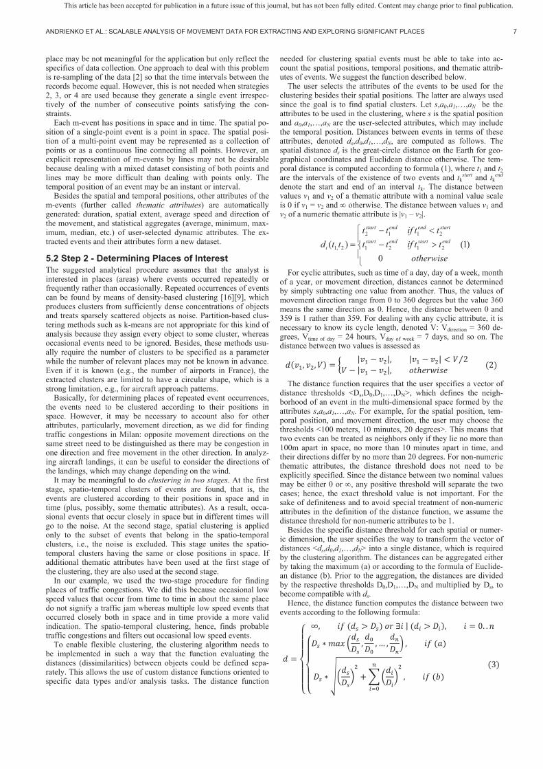
place may be not meaningful for the application but only reflect the specifics of data collection. One approach to deal with this problem is re-sampling of the data [2] so that the time intervals between the records become equal. However, this is not needed when strategies 2, 3, or 4 are used because they generate a single event irrespec-tively of the number of consecutive points satisfying the con-straints.
Each m-event has positions in space and in time. The spatial po-sition of a single-point event is a point in space. The spatial posi-tion of a multi-point event may be represented as a collection of points or as a continuous line connecting all points. However, an explicit representation of m-events by lines may not be desirable because dealing with a mixed dataset consisting of both points and lines may be more difficult than dealing with points only. The temporal position of an event may be an instant or interval.
Besides the spatial and temporal positions, other attributes of the m-events (further called thematic attributes) are automatically generated: duration, spatial extent, average speed and direction of the movement, and statistical aggregates (average, minimum, max-imum, median, etc.) of user-selected dynamic attributes. The ex-tracted events and their attributes form a new dataset.
5.2 Step 2 - Determining Places of Interest The suggested analytical procedure assumes that the analyst is interested in places (areas) where events occurred repeatedly or frequently rather than occasionally. Repeated occurrences of events can be found by means of density-based clustering [16][9], which produces clusters from sufficiently dense concentrations of objects and treats sparsely scattered objects as noise. Partition-based clus-tering methods such as k-means are not appropriate for this kind of analysis because they assign every object to some cluster, whereas occasional events need to be ignored. Besides, these methods usu-ally require the number of clusters to be specified as a parameter while the number of relevant places may not be known in advance. Even if it is known (e.g., the number of airports in France), the extracted clusters are limited to have a circular shape, which is a strong limitation, e.g., for aircraft approach patterns.
Basically, for determining places of repeated event occurrences, the events need to be clustered according to their positions in space. However, it may be necessary to account also for other attributes, particularly, movement direction, as we did for finding traffic congestions in Milan: opposite movement directions on the same street need to be distinguished as there may be congestion in one direction and free movement in the other direction. In analyz-ing aircraft landings, it can be useful to consider the directions of the landings, which may change depending on the wind.
It may be meaningful to do clustering in two stages. At the first stage, spatio-temporal clusters of events are found, that is, the events are clustered according to their positions in space and in time (plus, possibly, some thematic attributes). As a result, occa-sional events that occur closely in space but in different times will go to the noise. At the second stage, spatial clustering is applied only to the subset of events that belong in the spatio-temporal clusters, i.e., the noise is excluded. This stage unites the spatio-temporal clusters having the same or close positions in space. If additional thematic attributes have been used at the first stage of the clustering, they are also used at the second stage.
In our example, we used the two-stage procedure for finding places of traffic congestions. We did this because occasional low speed values that occur from time to time in about the same place do not signify a traffic jam whereas multiple low speed events that occurred closely both in space and in time provide a more valid indication. The spatio-temporal clustering, hence, finds probable traffic congestions and filters out occasional low speed events.
To enable flexible clustering, the clustering algorithm needs to be implemented in such a way that the function evaluating the distances (dissimilarities) between objects could be defined sepa-rately. This allows the use of custom distance functions oriented to specific data types and/or analysis tasks. The distance function
needed for clustering spatial events must be able to take into ac-count the spatial positions, temporal positions, and thematic attrib-utes of events. We suggest the function described below.
The user selects the attributes of the events to be used for the clustering besides their spatial positions. The latter are always used since the goal is to find spatial clusters. Let s,a0,a1,…,aN be the attributes to be used in the clustering, where s is the spatial position and a0,a1,…,aN are the user-selected attributes, which may include the temporal position. Distances between events in terms of these attributes, denoted ds,d0,d1,…,dN, are computed as follows. The spatial distance ds is the great-circle distance on the Earth for geo-graphical coordinates and Euclidean distance otherwise. The tem-poral distance is computed according to formula (1), where t1 and t2 are the intervals of the existence of two events and tk
start and tkend
denote the start and end of an interval tk. The distance between values v1 and v2 of a thematic attribute with a nominal value scale is 0 if v1 = v2 and otherwise. The distance between values v1 and v2 of a numeric thematic attribute is |v1 – v2|.
otherwisettifttttiftt
ttd endstartendstart
startendendstart
t
0)1()( 2121
2112
2,1
For cyclic attributes, such as time of a day, day of a week, month of a year, or movement direction, distances cannot be determined by simply subtracting one value from another. Thus, the values of movement direction range from 0 to 360 degrees but the value 360 means the same direction as 0. Hence, the distance between 0 and 359 is 1 rather than 359. For dealing with any cyclic attribute, it is necessary to know its cycle length, denoted V: Vdirection = 360 de-grees, Vtime of day = 24 hours, Vday of week = 7 days, and so on. The distance between two values is assessed as
The distance function requires that the user specifies a vector of distance thresholds <Ds,D0,D1,…,DN>, which defines the neigh-borhood of an event in the multi-dimensional space formed by the attributes s,a0,a1,…,aN. For example, for the spatial position, tem-poral position, and movement direction, the user may choose the thresholds <100 meters, 10 minutes, 20 degrees>. This means that two events can be treated as neighbors only if they lie no more than 100m apart in space, no more than 10 minutes apart in time, and their directions differ by no more than 20 degrees. For non-numeric thematic attributes, the distance threshold does not need to be explicitly specified. Since the distance between two nominal values may be either 0 or , any positive threshold will separate the two cases; hence, the exact threshold value is not important. For the sake of definiteness and to avoid special treatment of non-numeric attributes in the definition of the distance function, we assume the distance threshold for non-numeric attributes to be 1.
Besides the specific distance threshold for each spatial or numer-ic dimension, the user specifies the way to transform the vector of distances <ds,d0,d1,…,dN> into a single distance, which is required by the clustering algorithm. The distances can be aggregated either by taking the maximum (a) or according to the formula of Euclide-an distance (b). Prior to the aggregation, the distances are divided by the respective thresholds D0,D1,…,DN and multiplied by Ds, to become compatible with ds.
Hence, the distance function computes the distance between two events according to the following formula:
This article has been accepted for publication in a future issue of this journal, but has not been fully edited. Content may change prior to final publication.

8 IEEE TRANSACTIONS ON VISUALIZATION AND COMPUTER GRAPHICS, MANUSCRIPT ID
Option (a) defines the neighborhood of an event as a cube in the multi-dimensional space s,a0,a1,…,aN and option (b) as a sphere. In the latter case, two events will not be treated as neighbors when the distances d0,d1,…,dN do not reach the respective thresholds but are very close to them. This may be counter-intuitive; therefore, option (a) is preferable.
Distance function (3) is used for clustering by means of a densi-ty-based algorithm such as DBScan [16] or OPTICS [9].
Selection of thresholds is done based on analyst’s background knowledge of the physics of the movement, properties of the space where it takes place, characteristics of the data, and the goals of the analysis. Thus, the spatial and temporal distance thresholds should be much lower for cars slowly moving in a traffic jam than for landing aircraft. Suitable threshold values can be estimated using interactive visualizations of the extracted events. If the whole set of events does not fit in the RAM or cannot be efficiently handled by the visual and interactive tools, a sample or subset of the events is used. Note that spatial concentrations of events can be detected visually on a map where symbols representing events are drawn in a semi-transparent mode (figs. 1 and 11, right). The user can inter-actively vary the degree of transparency (e.g. by moving a slider) until the concentrations become well visible. Then the user can zoom in to several selected concentrations and measure the spatial distances from a few selected events to their third or fourth nearest neighbors. The maximum of these distances will give a suitable approximate value for the spatial distance threshold. In a similar way, the user can select the temporal threshold using a display of the events where one dimension represents time, e.g., dot plot, scatter plot, or STC [29]. To focus on events within spatial concen-trations, the user applies spatial filtering, e.g., by drawing a rectan-gle or another shape on a map around a group of symbols repre-senting the events. The filtering hides the events that are not in the enclosed area from all displays, which simplifies measuring the temporal distances between the events within the area. The same approach can also be used to select thresholds for other attributes; however, the semantics of the attributes often suggests suitable values. For instance, when cars move closely to each other on the same side of a city street, the directions can hardly differ by more than 20 degrees since sharp curves are not usual for city streets.
Still, the initial selection of the thresholds may be not good enough. When the thresholds are too high, the resulting clusters may be very large in space and/or time, e.g., a cluster of low speed events of cars may stretch over several streets and/or many hours. When the values are too low, the algorithm will find very few small clusters. Therefore, it is recommended to run clustering several times. Depending on the previous results, one of the thresholds is increased (if the clusters are small) or decreased (if the clusters are large) by a small amount, such as 10 to 25% of the previous value. To enable user’s evaluation of the clusters, they are visualized on a map and in an STC. The user checks if the cluster shapes and ex-tents in space and time are consistent with task-specific expecta-tions, e.g., elongated narrow clusters with the duration from 20 minutes to several hours in searching for traffic jams.
After the user is satisfied with the clustering results, spatial buff-ers or convex hulls are constructed around the clusters. These areas represent the places of interest that have been sought for.
In the examples presented in sections 4 and 7, we selected the thresholds for the clustering in the way described above. For the brevity sake, we do not describe all trials of the clustering but report only the finally chosen threshold values.
5.3 Step 3 - Aggregating Events and Trajectories Spatio-temporal aggregation of events is used for studying the temporal patterns of event occurrences in different places [18]. For the aggregation, the user divides the time span of the data into suitable intervals based on the linear or cyclic time model. In the latter case, the user selects one of the temporal cycles: daily, week-ly, or yearly. The cycle is divided into intervals. Events whose times fit in the same interval of the cycle are grouped together
irrespectively of their absolute temporal positions, which may be one or more cycles apart.
The aggregation groups together events with the spatial positions being in the same place and temporal positions in the same interval. For each group of events (i.e., for each combination of place and interval), the count of the events is computed as well as the count of different moving objects and statistics of the event attributes such as duration, movement speed, direction, etc. These values are attached to the places as dynamic (time-dependent) attributes. Hence, each place is characterized by a time series of values of each count and aggregate attribute.
Spatio-temporal aggregation can also be applied to trajectories [1]. Two kinds of aggregates can be obtained: aggregates characterizing each place: number of visits of the
place, number of different visitors, statistics of the durations of staying within the place, movement speeds, directions, etc.;
aggregates characterizing links between the places: number of moves from place A to place B, number of different objects that moved from A to B, statistics of the path lengths, durations, speeds, etc.
Aggregates of the first kind are computed for every place by user-defined time intervals. As a result, the place is characterized by a time series of values of each attribute. Aggregates of the second kind are computed for every pair of places. For a pair of places A and B, trajectories that visit B immediately after A (i.e., no other relevant place is visited in between) are selected. The time interval between the last position in A and the first position in B is matched to the user-specified time intervals. If the interval of the move from A to B lies fully within some of the predefined intervals, the move is added to the statistics for this interval. In other cases, the interval that contains the largest part of the time of the move is chosen. Pairs of places for which there are no connecting moves are dis-carded. The result is a set of aggregate moves, or flows [4][36]. Geometrically, a flow is a vector connecting place A to place B. It is associated with a time series of values of each computed aggre-gate attribute. For each place, the incoming and outgoing flows characterize this place in terms of its links to other places.
Besides the time series, places and flows may be characterized by static attributes representing the total numbers of events, visits, visitors, and other statistics for the whole time span of the data.
5.4 Step 4 - Analysis of Aggregated Data The main result of the aggregation step is time series of attribute values associated with the relevant places or flows between the places. There are many methods that can be used for analyzing spatially referenced time series, including spatial and non-spatial interactive visualizations [1][11] and computational methods from statistics [24] and data mining [34]. We have demonstrated some possibilities in section 4; some other methods will be applied in the example in section 7.
6 SCALABILITY OF THE PROCEDURE Here we describe how the suggested procedure can be scaled to very large datasets which, possibly, do not fully fit in the RAM. We used a recently developed scalable implementation of the procedure to analyze the Milan traffic data in section 4. Without it, it was only possible to analyze a subset of the data from one day, as in [3], but not the whole dataset spanning over a week.
6.1 Scalable Event Extraction Relational databases do not provide the necessary data types and functions for dealing with mobility data. Database researchers are now developing specialized moving object databases (MOD), which can compute various dynamic attributes of trajectories and fulfill sophisticated queries for event extraction [21]. A possible scenario for integrating interactive visual query tools with the power of MOD may be as follows.
This article has been accepted for publication in a future issue of this journal, but has not been fully edited. Content may change prior to final publication.

ANDRIENKO ET AL.: SCALABLE ANALYSIS OF MOVEMENT DATA FOR EXTRACTING AND EXPLORING SIGNIFICANT PLACES 9
Cumulative curves can be built without loading the original data in the RAM since the necessary aggregation can be done within the database. Frequencies and cumulated values of selected quantita-tive attributes are calculated for small value intervals of the base attribute (e.g. one thousandth of the whole value range). The results are loaded in the RAM and used for building the curves, which are used to select several candidate threshold values. The spatial and temporal distributions of the potential m-events for these values can be assessed with the help of spatio-temporal aggregation. For small territory compartments and short time intervals, the frequen-cies of values from the defined intervals are counted in the data-base, loaded in the RAM and visualized on a map and in a space-time cube. Observing the spatio-temporal distribution of the fre-quencies allows the analyst to make the final choice of the suitable threshold values and build a query, which is then fulfilled in the MOD. The query creates a set of event objects with attributes. If the set is too large for processing within the RAM, the event clus-tering is done as described below.
6.2 Scalable Event Clustering We suggest an approach to applying a density-based clustering algorithm such as DBSCAN or OPTICS to a set of events not fitting in RAM. Density-based clustering is built upon the opera-tion of finding the neighbors of a given object, i.e., such objects whose distances to the given object are within the distance thresh-old. Our approach involves a pre-clustering scan of the set of events in which lists of the neighbors of all events are created and stored in the database, to be later retrieved on demand in the course of the clustering. During the pre-clustering, only a small subset of events needs to be present in RAM at each moment. The approach exploits the capabilities of the database management system and the properties of the distance function.
According to formula (3), the distance between two events is in-finite if at least one of the distances ds, d0, d1, …, dN exceeds the respective threshold from the multi-dimensional threshold vector <Ds,D0,D1,…,DN>. We decompose the spatial dimension into two dimensions x and y or three dimensions x, y, and z in case of three-dimensional space. The distance ds can be within the threshold Ds only if each of the distances dx, dy and dz does not exceed Ds. An event e can be represented by a tuple <c1
e,c2e,…,cM
e> where each component ci {x,y,z,a0,a1,…,aN} is scalar. Let <D1,D2,…,DM> be the vector of distance thresholds for the dimensions c1,c2,…,cM, respectively. We define the relevant zone (RZ) of event e in dimen-sion ci as the interval [ci
e-Di,cie+Di], where ci
e is the value of di-mension ci for the event e. Let us consider the projection of all events onto the dimension ci. By definition of the distance function (3), two events cannot be neighbors if one of them is not contained within the RZ of the other. This holds for any dimension c1,c2,…,cM. Hence, any event has a set of relevant zones, one in each dimension, and each RZ contains all neighbors of the event. Consequently, in order to find the neighbors of an event, it is suffi-cient to search in one of its relevant zones. It is advantageous to use the RZ containing the least number of events.
Our approach exploits the relevant zones of the events for ex-tracting their neighbors in a scalable while efficient way. The key idea is that for a given event only the events from one of its RZ need to be present in the RAM; moreover, as will be shown later, one half of the RZ is sufficient. We shall use the terms lower rele-vant zone (LRZ) and upper relevant zone (URZ) to refer, respec-tively, to the lower and upper halves of the interval [ci
e-Di,cie+Di]:
LRZ [cie-Di, ci
e] and URZ [cie ci
e+Di]. Note that if event ej belongs to the LRZ of event ek then necessarily ek belongs to the URZ of ei, and vice versa.
For the pre-clustering, one of the dimensions c1,c2,…,cM is cho-sen for defining relevant zones. The choice of the most suitable dimension will be discussed later on. The events are sorted in the database in the ascending order of the values of the chosen dimen-sion cj and then processed in this order. The following operations are iteratively performed (Algorithm 1):
1. The next event ek is loaded in the RAM and associated with an empty list of neighbors.
2. Each event ei present in the RAM is checked against ek: 2.1. If ei LRZ(ek) then ei with its list of neighbors is unloaded
from the RAM to the database. 2.2. Otherwise, the distance d between ei and ek is computed ac-
cording to formula (3). If d<Ds, i.e., ei and ek are neighbors, then the pair (ek,d) is inserted in the list of neighbors of ei and the pair (ei,d) is inserted in the list of neighbors of ek.
At the end, all events that still remain in the RAM are unloaded with their lists of neighbors to the database. The lists of neighbors can be ordered by the distances. The output of the algorithm is a database table containing for each event its list of neighbors, possi-bly, empty. In the following clustering, the events having no neigh-bors are ignored, which increases the efficiency of the clustering.
At each iteration step of Algorithm 1, the RAM contains events only from the LRZ of the currently processed event ek but not from its URZ. However, the events from the URZ will be loaded later and the list of neighbors of ek will be updated when necessary while ek is still in the RAM. Unloading of ek from the RAM means that it is outside of the LRZ of the next event. Due to the ordering, none of the following events can be a neighbor of ek.
The work of Algorithm1 is illustrated in fig. 9. Events are repre-sented by points in two dimensions. The neighborhood areas of the events are represented by circles around the points. The horizontal dimension (x) is used for ordering and defining the relevant zones. The LRZ of the currently processed event is marked in each step by a gray-shaded rectangle. For events 1 and 2, the LRZs contain no other events. For event 3, the LRZ contain event 2; however, the distance between 2 and 3 exceeds the threshold, i.e., these events are not neighbors. Event 4 has events 2 and 3 in its LRZ and its distances to these events are below the threshold. Hence, the lists of neighbors of all three events 2, 3, and 4 are updated. The lists of events 2 and 3 include 4 and the list of event 4 includes 2 and 3.
There is a special case when a cyclic attribute, such as direction, is chosen for defining relevant zones of events. When events are ordered based on the values of a cyclic attribute, the LRZs of the first events in the sequence may contain events that are positioned at the end of the list. When the last events are processed, the first events are no more in the RAM. Hence, the first events cannot be attached to the neighbor list of the last events and their own neigh-bor lists cannot be updated. To deal with this problem, Algorithm 1 is modified as follows.
Let Acyc be the cyclic attribute used for event ordering, V its cy-cle length, D the distance threshold, and v0 the value of Acyc for the first event in the list e0. Before starting Algorithm 1, all events from the end of the list that belong to the LRZ of e0, i.e., {ek | vk v0 + V – D}, are pre-loaded to the RAM and marked as “transient”. The special mark distinguishes them from the other events that will
Fig. 9. Illustration of event pre-clustering. The events, represented as two-dimensional points, are ordered according to the x dimension. The neighborhood areas are represented by circles. The lower rele-vant zone in each step is marked with a gray rectangle.
This article has been accepted for publication in a future issue of this journal, but has not been fully edited. Content may change prior to final publication.

10 IEEE TRANSACTIONS ON VISUALIZATION AND COMPUTER GRAPHICS, MANUSCRIPT ID
be loaded during step 1 of Algorithm 1. Let e1t denote the first
transient event from all transient events ordered according to Acyc. Before unloading an event ei at step 2.1, it is checked if ei is
marked as “transient”. If so, it is unloaded with its neighbor list to a special buffer B, otherwise to the database, as usual.
When at step 1 the event e1t and its successive events, i.e. the last
events from the list, are loaded in the RAM, their neighbor lists are initialized with the lists stored in the buffer B. Since B has the same order of the incoming events, the retrieval of the lists is per-formed in constant time.
Let be the number of events in the input dataset and the maximum number of events in the LRZ of one event. The com-plexity of Algorithm 1 is O(n log n + n N), where n log n time is used for the ordering and n N for checking all events against the events from their lower relevant zones. The complexity may be quadratic in the worst case when N=O(n), i.e., one event contains almost all other events in its LRZ. This means that the distance threshold for the chosen ordering dimension is close to the whole range of this dimension. In most cases, however, the ordering dimension can be chosen so that N<<n, which reduces the com-plexity to (n log n). Using the capabilities of DBMS, it is possible to retrieve the sequence of events already sorted according to the chosen dimension. In this case, the sorting cost is externalized to the database and the resulting complexity is reduced to (n).
The choice of the most suitable ordering dimension is based on two criteria. First, the average number of events in a LRZ of one event should be as small as possible. Second, the maximal number of events in a LRZ should not exceed the RAM capacity. In order to estimate the average and maximal number of events in a LRZ in each dimension, a frequency histogram for each dimension is built using the database facilities. The appropriate width of the histo-gram bin is one half of the distance threshold for this dimension.
Still, even an optimal choice of the ordering dimension cannot guarantee that the events that need to be processed at each step of Algorithm 1 will always fit in the RAM. If at some step the events from the LRZ of the currently processed event do not fit in the RAM, they are offloaded to an external buffer and the process continues using this buffer instead on the RAM. The overhead of accessing the data on the disk will decrease the performance, but the buffer removes the constraint on the memory size. As soon as the size of the buffer content becomes suitable for the RAM, it is moved to the main memory for more efficient access.
After the pre-clustering phase is concluded, clusters of events are determined by means of the clustering algorithm. The algorithm requires the extraction of the neighbors of each event, which has already been done. Hence, the list of neighbors just needs to be loaded from the database. The memory complexity of the cluster-ing is bounded by the maximum number of neighbors of one event.
Using the set of the 251,588 low speed events extracted from the Milan car trajectories (see section 4), we have performed four computational experiments using longitude, latitude, time and direction as the ordering dimensions. The results are summarized in Table 1, where ‘RZ size’ means the number of events in the RZ. The completion time includes also the time of clustering.
Table 1. RAM requirements and computation times depending on the choice of the ordering dimension.
Dimension Average RZ size
Minimal RZ size
Maximal RZ size
Completion time (sec)
Longitude 1137 0 2517 150 Latitude 1254 0 7541 167 Time 1626 0 3554 196 Direction 15539 7943 32579 2346
The experiments have been conducted on a PC with 24GB of RAM, which also allowed loading and clustering of all low speed events in the RAM. A sole application of the OPTICS algorithm to the events loaded in the RAM takes 5 hours 38 minutes and 18 seconds. With the use of a spatial index of the events (R-tree [22]), the clustering is done in 55 seconds, but the RAM capacity is fully
consumed and clustering of 300,000 or more events would be impossible. The use of Algorithm 1 radically decreases the RAM demand while the computation time does not increase too much.
Table 1 shows that the computation time and RAM demand greatly depend on the choice of the ordering dimension. For the Milan example, the best choice is longitude. The choice of direc-tion increases the computation time by the factor of 20. As the ratio between the directional distance threshold (20) and the attribute value range (360) is quite large, the LRZ of each event contains too many events that need to be checked in step 2 of Algorithm 1. The variation of the RZ sizes in the course of performing Algorithm 1 using different event orderings is presented graphically in fig.10.
Earlier [3] we have suggested a method for scalable clustering of spatial events based on temporal ordering of the events and using a sliding time window for loading event subsets in the RAM; more details are given in [33]. The method presented here generalizes the idea of time window and allows replacing time by other attributes, which can improve the performance, as in the case of Milan data.
6.3 Further Processing and Analysis Spatial buffers or convex hulls around spatial clusters of events can be built in a spatial database, e.g., Oracle Spatial. The spatio-temporal aggregation can also be done in the database, and only the resulting aggregates loaded in the RAM for visualization and ex-ploration.
Hence, all steps of the suggested procedure can be done without loading all data simultaneously in the RAM. We have used this opportunity in the example presented in section 4. The following section describes another example of using the procedure. Alt-hough in this case the data allow processing in the RAM, we use the example to demonstrate analysis on a different spatial scale and characterizing extracted places in terms of links between them.
7 ANALYZING FLIGHTS DYNAMICS IN FRANCE Analysis of air traffic is essential for improving the aviation safety and optimizing the use of airports and flight routes. Air traffic control (ATC) data, which contain trajectories of aircraft, are col-lected by radars. These datasets contain lots of tangled trails that are difficult to explore. Previous work [26] managed to manually extract certain kinds of information with the direct manipulation paradigm. In this case study, we shall apply our visual analytics procedure to ATC data with the following goals: 1. Identify the airports in use. 2. Investigate the temporal dynamics of the flights to and from the
airports (i.e., landings and takeoffs). 3. Investigate the connections among the airports, the intensity of
the flights between them, and their distribution over a day. We use a dataset with 17,851 flight trajectories over France dur-
ing one day (Friday, the 22nd of February, 2008) consisting of
Fig. 10. The graphs depict the variation of the RZ sizes in the course of scanning of the list of low speed events in Milan ordered accord-ing to longitude (red), latitude (blue), time (green), and direction (brown). Top: the Y-axis is linear. Bottom: the Y-axis is logarithmic.
This article has been accepted for publication in a future issue of this journal, but has not been fully edited. Content may change prior to final publication.

ANDRIENKO ET AL.: SCALABLE ANALYSIS OF MOVEMENT DATA FOR EXTRACTING AND EXPLORING SIGNIFICANT PLACES 11
427,651 records. The trajectories, shown in fig. 11 left, include flights of passenger, cargo, and private airplanes and helicopters. The temporal resolution of the data mostly varies from 1 to 3 minutes, although larger time gaps (up to 5 minutes) also occur.
It may not be obvious to the reader why the airport areas need to be determined from the data instead of using the official airport boundaries, which should be known. The problem is the low tem-poral resolution of the data. For many flights, the first recorded positions lie outside the boundaries of the origin airports and/or the last recorded positions are not within the boundaries of the destina-tion airports. Therefore, to refer the flights to their origin and desti-nation airports, it is necessary to build sufficiently large areas around the airports that would include the available first and last points. It is not known in advance how large the areas need to be and what geometrical shapes are appropriate.
Our approach to defining the areas is based on the background knowledge that airplanes typically land and take off in similar directions, which are determined by the orientation of the airport runways. We extract the available last positions of the aircraft that landed and first positions of those that took off and cluster them by spatial positions and movement directions. As a result, points lying outside or even quite far from the airports are grouped together with the points lying within the airport boundaries if they corre-spond to landings or takeoffs with similar directions. The airport “catchment” areas are built as buffers around these clusters. The
areas can be verified using the known positions of the airports: they must be within the areas.
Not always starts and ends of trajectories correspond to takeoffs and landings. The radar observation data also contain parts of transit trajectories that just pass over France as well as flights going outside France and those coming to France from abroad. Real takeoffs and landings must be distilled from the available starts and ends of the recorded tracks. To extract the landings, we use the following query condition: the altitude is less than 1 km in the last 5 minutes of the trajectory. From each trajectory that has such points, we extract the last point as the m-event representing the landing (fig. 11 right). Then we cluster the landing events by the spatial positions and directions using the thresholds of 1km and 30 degrees, respectively. The resulting SD-clusters are presented in the STC in fig. 12; the noise is excluded. The colors represent different clusters. The vertical alignments of points correspond to the airports where multiple landings took place during the day.
An interesting pattern can be observed in the area of Nice on the southeast of France. There are two SD-clusters of landings, yellow and green; their points make a column on the right in the cube. The green cluster appears as an intrusion inside the yellow one. This means that the landing direction changed in this area twice during the day, perhaps, due to a change of the wind (airplanes take off and land facing the wind). The map fragment in fig. 13 shows that the yellow cluster contains landings from the southwest and the green cluster landings from the northeast. The blue lines show the
Fig. 11. The trajectories are drawn with 1% opacity (left). The posi-tions of the landing events extracted from the flight data are drawnwith 50% opacity (right).
Fig. 12. The space-time cube shows the landing events clustered byspatial positions and directions.
Fig. 13. The yellow and green dots represent two SD-clusters of landings in the airport of Nice. The time diagrams show the dynam-ics of the landings from two directions.
Fig. 14. The time diagrams show the dynamics of landings in the airports of Paris.
This article has been accepted for publication in a future issue of this journal, but has not been fully edited. Content may change prior to final publication.

12 IEEE TRANSACTIONS ON VISUALIZATION AND COMPUTER GRAPHICS, MANUSCRIPT ID
last ten minutes fragments of the respective trajectories and reflect the mandatory landing directions.
The observation of the direction changes gives us an idea that the temporal patterns of landings should be investigated not by airports only but by airports and landing directions. Therefore, we build 500-meter spatial buffers around the SD-clusters, as shown in fig. 13. For an analysis by airports, irrespective of the directions, we would do a second stage of clustering (after excluding the noise) by only the spatial positions of the events and then build buffers around the resulting S-clusters.
In the third step, we aggregate the landing events in space by the buffers and in time by one-hour intervals. In the fourth step, we visualize the resulting time series by temporal diagrams drawn on the map display; two of them can be seen in fig. 13. They show that the aircraft landed in the airport of Nice from the southwest almost all time except for an interval in the middle of the day, when the landing direction changed to the opposite. The exact times and values are displayed when the mouse cursor points on an area.
Figure 14 presents a map fragment with the temporal diagrams for the Paris region. We can see that the Orly airport and the north-ern runway of the Charles de Gaulle (CDG) airport have peaks in the morning and in the evening. It is a typical pattern for airline hubs: short period of time, during which many fights arrive and take off, maximize the number of possible connections. The south-ern runway of the CDG airport is used with almost constant intensi-ty during the day. The remaining airports are used much less inten-sively and mostly in the afternoon.
This pattern can be explained as follows. The CDG airport has two pairs of runways: 2 north and 2 south runways, and two main terminals, south and north. For ground traffic optimization purpos-es, airplanes which need to park at the south terminal prefer to land on the south runway. The same applies to the north terminal and north runway. The north terminal and runways are used by foreign companies. It is very busy in the morning when transatlantic flights arrive; then the traffic decreases. The south terminal and runways are mainly used by French companies and the south terminal is three times bigger than the north one. Therefore the traffic is more intensive along the day.
So far we have considered only the landings. To investigate the takeoffs, we repeat the procedure. To extract the takeoff events in the first step, we use the query condition that the altitude must be less than 1 km at the beginning of the trajectory. The remainder of the procedure is similar to that for the landings.
To investigate the links between the airports, we need to define the airport areas so that they include both the takeoff and the land-ing events. We join the sets of the takeoff and landing events, which have been previously filtered by removing the noise after the SD-clustering. Then we apply clustering by spatial positions, to unite the clusters of takeoffs and landings in different directions occurring at the same airports. We build spatial buffers around the S-clusters to obtain the airport areas. In the third step, we aggregate the trajectories by pairs of places (airport areas) and time intervals (1 hour length), as described in section 5.3. We use only the trajec-tories having both takeoff and landing events. As a result, we ob-tain aggregate flows (vectors) with respective hourly time series and totals of flight counts.
To investigate the aggregates, we visualize the total counts on a flow map. The flows are shown by directed arrows with the widths proportional to the flight counts. By interactive filtering, we hide minor flows (less than 5 flights) and focus on the short-distance flows (below 100 km distance). In the upper part of fig. 15, short-distance flows are shown for the region of Paris and its suburbs. We see that there are quite many flights connecting close airports, particularly, in Paris. As explained by a domain expert, a part of them are flights without passengers used for relocating aircraft between big airports, such as CDG and Orly. Short-distance flows between small airports correspond to training and leisure flights of private pilots.
To investigate movements between the cities of France, we in-teractively edit the S-clusters of takeoffs and landings; namely, we unite the clusters located within Paris into a single cluster. We again build spatial buffers around the clusters and aggregate the trajectories as before. The resulting flows are shown in the flow
Fig. 15. Connections between airports in Paris (top) and betweencities (bottom) are shown by directed arrows with the widths propor-tional to the total flight counts.
Fig. 16. The distribution of the flights between the cities by hourly intervals is represented in a table lens display. Highlighted are rows for the connections Toulouse-Paris (blue) and Paris-Toulouse (or-ange). At the bottom, the two highlighted rows are shown in detail.
This article has been accepted for publication in a future issue of this journal, but has not been fully edited. Content may change prior to final publication.
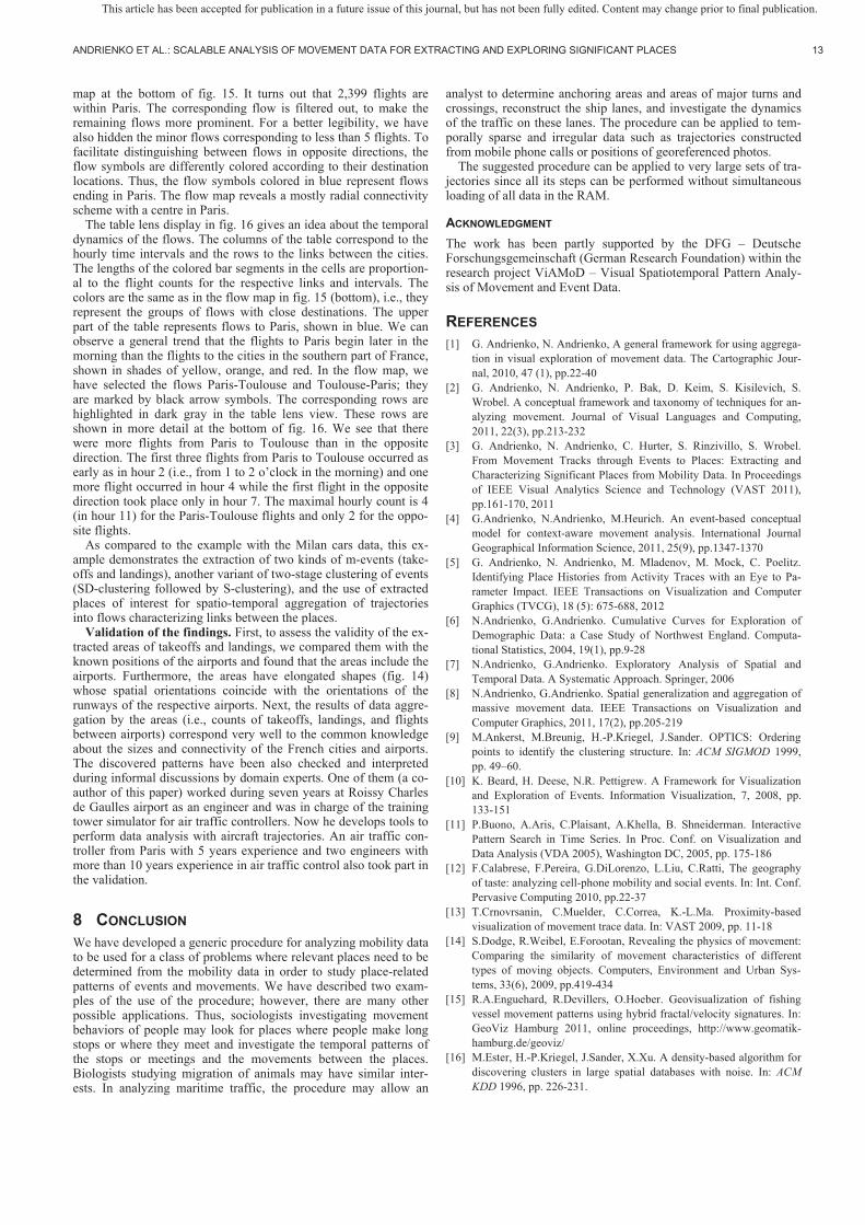
ANDRIENKO ET AL.: SCALABLE ANALYSIS OF MOVEMENT DATA FOR EXTRACTING AND EXPLORING SIGNIFICANT PLACES 13
map at the bottom of fig. 15. It turns out that 2,399 flights are within Paris. The corresponding flow is filtered out, to make the remaining flows more prominent. For a better legibility, we have also hidden the minor flows corresponding to less than 5 flights. To facilitate distinguishing between flows in opposite directions, the flow symbols are differently colored according to their destination locations. Thus, the flow symbols colored in blue represent flows ending in Paris. The flow map reveals a mostly radial connectivity scheme with a centre in Paris.
The table lens display in fig. 16 gives an idea about the temporal dynamics of the flows. The columns of the table correspond to the hourly time intervals and the rows to the links between the cities. The lengths of the colored bar segments in the cells are proportion-al to the flight counts for the respective links and intervals. The colors are the same as in the flow map in fig. 15 (bottom), i.e., they represent the groups of flows with close destinations. The upper part of the table represents flows to Paris, shown in blue. We can observe a general trend that the flights to Paris begin later in the morning than the flights to the cities in the southern part of France, shown in shades of yellow, orange, and red. In the flow map, we have selected the flows Paris-Toulouse and Toulouse-Paris; they are marked by black arrow symbols. The corresponding rows are highlighted in dark gray in the table lens view. These rows are shown in more detail at the bottom of fig. 16. We see that there were more flights from Paris to Toulouse than in the opposite direction. The first three flights from Paris to Toulouse occurred as early as in hour 2 (i.e., from 1 to 2 o’clock in the morning) and one more flight occurred in hour 4 while the first flight in the opposite direction took place only in hour 7. The maximal hourly count is 4 (in hour 11) for the Paris-Toulouse flights and only 2 for the oppo-site flights.
As compared to the example with the Milan cars data, this ex-ample demonstrates the extraction of two kinds of m-events (take-offs and landings), another variant of two-stage clustering of events (SD-clustering followed by S-clustering), and the use of extracted places of interest for spatio-temporal aggregation of trajectories into flows characterizing links between the places.
Validation of the findings. First, to assess the validity of the ex-tracted areas of takeoffs and landings, we compared them with the known positions of the airports and found that the areas include the airports. Furthermore, the areas have elongated shapes (fig. 14) whose spatial orientations coincide with the orientations of the runways of the respective airports. Next, the results of data aggre-gation by the areas (i.e., counts of takeoffs, landings, and flights between airports) correspond very well to the common knowledge about the sizes and connectivity of the French cities and airports. The discovered patterns have been also checked and interpreted during informal discussions by domain experts. One of them (a co-author of this paper) worked during seven years at Roissy Charles de Gaulles airport as an engineer and was in charge of the training tower simulator for air traffic controllers. Now he develops tools to perform data analysis with aircraft trajectories. An air traffic con-troller from Paris with 5 years experience and two engineers with more than 10 years experience in air traffic control also took part in the validation.
8 CONCLUSION We have developed a generic procedure for analyzing mobility data to be used for a class of problems where relevant places need to be determined from the mobility data in order to study place-related patterns of events and movements. We have described two exam-ples of the use of the procedure; however, there are many other possible applications. Thus, sociologists investigating movement behaviors of people may look for places where people make long stops or where they meet and investigate the temporal patterns of the stops or meetings and the movements between the places. Biologists studying migration of animals may have similar inter-ests. In analyzing maritime traffic, the procedure may allow an
analyst to determine anchoring areas and areas of major turns and crossings, reconstruct the ship lanes, and investigate the dynamics of the traffic on these lanes. The procedure can be applied to tem-porally sparse and irregular data such as trajectories constructed from mobile phone calls or positions of georeferenced photos.
The suggested procedure can be applied to very large sets of tra-jectories since all its steps can be performed without simultaneous loading of all data in the RAM.
ACKNOWLEDGMENT The work has been partly supported by the DFG – Deutsche Forschungsgemeinschaft (German Research Foundation) within the research project ViAMoD – Visual Spatiotemporal Pattern Analy-sis of Movement and Event Data.
REFERENCES [1] G. Andrienko, N. Andrienko, A general framework for using aggrega-
tion in visual exploration of movement data. The Cartographic Jour-nal, 2010, 47 (1), pp.22-40
[2] G. Andrienko, N. Andrienko, P. Bak, D. Keim, S. Kisilevich, S. Wrobel. A conceptual framework and taxonomy of techniques for an-alyzing movement. Journal of Visual Languages and Computing, 2011, 22(3), pp.213-232
[3] G. Andrienko, N. Andrienko, C. Hurter, S. Rinzivillo, S. Wrobel. From Movement Tracks through Events to Places: Extracting and Characterizing Significant Places from Mobility Data. In Proceedings of IEEE Visual Analytics Science and Technology (VAST 2011), pp.161-170, 2011
[4] G.Andrienko, N.Andrienko, M.Heurich. An event-based conceptual model for context-aware movement analysis. International Journal Geographical Information Science, 2011, 25(9), pp.1347-1370
[5] G. Andrienko, N. Andrienko, M. Mladenov, M. Mock, C. Poelitz. Identifying Place Histories from Activity Traces with an Eye to Pa-rameter Impact. IEEE Transactions on Visualization and Computer Graphics (TVCG), 18 (5): 675-688, 2012
[6] N.Andrienko, G.Andrienko. Cumulative Curves for Exploration of Demographic Data: a Case Study of Northwest England. Computa-tional Statistics, 2004, 19(1), pp.9-28
[7] N.Andrienko, G.Andrienko. Exploratory Analysis of Spatial and Temporal Data. A Systematic Approach. Springer, 2006
[8] N.Andrienko, G.Andrienko. Spatial generalization and aggregation of massive movement data. IEEE Transactions on Visualization and Computer Graphics, 2011, 17(2), pp.205-219
[9] M.Ankerst, M.Breunig, H.-P.Kriegel, J.Sander. OPTICS: Ordering points to identify the clustering structure. In: ACM SIGMOD 1999, pp. 49–60.
[10] K. Beard, H. Deese, N.R. Pettigrew. A Framework for Visualization and Exploration of Events. Information Visualization, 7, 2008, pp. 133-151
[11] P.Buono, A.Aris, C.Plaisant, A.Khella, B. Shneiderman. Interactive Pattern Search in Time Series. In Proc. Conf. on Visualization and Data Analysis (VDA 2005), Washington DC, 2005, pp. 175-186
[12] F.Calabrese, F.Pereira, G.DiLorenzo, L.Liu, C.Ratti, The geography of taste: analyzing cell-phone mobility and social events. In: Int. Conf. Pervasive Computing 2010, pp.22-37
[13] T.Crnovrsanin, C.Muelder, C.Correa, K.-L.Ma. Proximity-based visualization of movement trace data. In: VAST 2009, pp. 11-18
[14] S.Dodge, R.Weibel, E.Forootan, Revealing the physics of movement: Comparing the similarity of movement characteristics of different types of moving objects. Computers, Environment and Urban Sys-tems, 33(6), 2009, pp.419-434
[15] R.A.Enguehard, R.Devillers, O.Hoeber. Geovisualization of fishing vessel movement patterns using hybrid fractal/velocity signatures. In: GeoViz Hamburg 2011, online proceedings, http://www.geomatik-hamburg.de/geoviz/
[16] M.Ester, H.-P.Kriegel, J.Sander, X.Xu. A density-based algorithm for discovering clusters in large spatial databases with noise. In: ACM KDD 1996, pp. 226-231.
This article has been accepted for publication in a future issue of this journal, but has not been fully edited. Content may change prior to final publication.

14 IEEE TRANSACTIONS ON VISUALIZATION AND COMPUTER GRAPHICS, MANUSCRIPT ID
[17] A.Frank. Qualitative spatial reasoning about distances and directions in geographical space. Journal of Visual Languages and Computing, 1992, 3, pp. 343-371
[18] A.Fredrikson, C.North, C.Plaisant, B.Shneiderman. Temporal, geo-graphical and categorical aggregations viewed through coordinated displays: a case study with highway incident data. In Proc. Workshop on New Paradigms in information Visualization and Manipulation. ACM, 1999, 26-34.
[19] F.Giannotti, M.Nanni, F.Pinelli, D.Pedreschi. Trajectory pattern mining. In: KDD 2007, pp. 330–339
[20] H.Guo, Z.Wang, B.Yu, H.Zhao, X.Yuan. TripVista: Triple perspec-tive visual trajectory analytics and its application on microscopic traf-fic data at a road intersection. In: PacificVis 2011, pp. 163-170
[21] R.H.Güting, M.Schneider. Moving Objects Databases. Morgan Kauf-mann, 2005.
[22] A. Guttman, R-Trees: A Dynamic Index Structure for Spatial Search-ing. In Proceedings of the 1984 ACM SIGMOD international confer-ence on Management of data (SIGMOD '84), pp. 47-57, 1984
[23] T.Hägerstrand. What about people in regional science? Papers, Re-gional Science Association, 24, 1970, pp. 7-21.
[24] J.D.Hamilton. Time series analysis. Princeton University Press, 1994 [25] M.Harrower, C.A.Brewer: Colorbrewer.org: An online tool for
selecting color schemes for maps. The Cartographic Journal 40(1): 27–37, 2003.
[26] C.Hurter, B.Tissoires, S.Conversy. FromDaDy: Spreading aircraft trajectories across views to support iterative queries. IEEE Transac-tions on Visualization and Computer Graphics, 15(6), 2009, pp. 1017-1024
[27] P.Kalnis, N.Mamoulis, S.Bakiras. On discovering moving clusters in spatio-temporal data. In: Advances in spatial and temporal databases 2005. LNCS 3633, 364-381
[28] J. Kim. Events as property exemplifications. In: M.Brand, D.Walton (eds.). Action Theory, Reidel, Dordrecht, 1976, pp. 159–177
[29] M.-J.Kraak, The space-time cube revisited from a geovisualization perspective. In: Proc. 21st Int. Cartographic Conference, Durban, 2003, pp.1988-1995
[30] P.Laube, S.Imfeld, R.Weibel. Discovering relative motion patterns in groups of moving point objects. International Journal Geographic In-formation Science, 19(6), 2005, pp. 639–668
[31] P.A.Longley, M.F.Goodchild, D.J.Maguire, D.W.Rhind. Geographical Information Systems. Vol. 1: Principles and Technical Issues, Second Edition, John Wiley & Sons, New York, USA, 1999
[32] J.Macedo, C.Vangenot, W.Othman, N.Pelekis, E.Frentzos, B.Kuijpers, I.Ntoutsi, S.Spaccapietra, Y.Theodoridis. Trajectory data models. In F.Giannotti & D.Pedreschi (eds.). Mobility, Data Mining and Privacy - Geographic Knowledge Discovery, Springer, Berlin, 2008, pp. 123-150
[33] I. Peca, G. Fuchs, K. Vrotsou, N. Andrienko, G. Andrienko. Scalable Cluster Analysis of Spatial Events. In: Proceedings of International Workshop on Visual Analytics (EuroVA 2012), pp.19-23
[34] J.F.Roddick, M.Spiliopoulou. A survey of temporal knowledge dis-covery paradigms and methods. IEEE Transactions on Knowledge and Data Engineering, 14(4), 2002, pp. 750-767
[35] R.Scheepens, N.Willems, H. van de Wetering, J.J. van Wijk. Interac-tive visualization of multivariate trajectory data with density maps. In: PacificVis 2011, pp. 147-154
[36] J.Wood, J.Dykes, A.Slingsby, Visualization of origins, destinations and flows with OD maps. The Cartographic Journal, 2010, 47(2), pp.117-129
[37] M.F.Worboys. Event-oriented approaches to geographic phenomena. International Journal of Geographic Information Science, 19(1), 2005, pp. 1-28
[38] Z.Yan, J.Macedo, C.Parent, S.Spaccapietra. Trajectory Ontologies and Queries. Transactions in GIS, 12(1), 2008, pp. 75 – 91
Gennady Andrienko is a lead scientist respon-sible for the visual analytics research at the Fraunhofer Institute for Intelligent Analysis and Information Systems (IAIS). He co-authored the monograph ‘Exploratory Analysis of Spatial and Temporal Data’ (Springer, 2006), 50+ peer-reviewed journal papers, 20+ book chapters and more than 100 conference papers. Since 2007, Gennady Andrienko is chairing the ICA Commis-
sion on GeoVisualization. He co-organized scientific events on visual analytics, geovisualization and visual data mining, and co-edited 10 special issues of journals.
Natalia Andrienko has been working at GMD, now Fraunhofer IAIS, since 1997. Since 2007, she is a lead scientist responsible for the visual analytics research. She co-authored the mono-graph ‘Exploratory Analysis of Spatial and Tem-poral Data’, over 50 peer-reviewed journal pa-pers, over 20 book chapters and more than 100 conference papers. She received best paper awards at the AGILE 2006 and IEEE VAST 2011
and 2012 conferences, best poster awards at AGILE 2007 and ACM GIS 2011, and VAST challenge award 2008.
Christophe Hurter is a researcher at ENAC (Ecole Nationale de l’Aviation Civile), in Toulouse France. He teaches and conducts research into Human-Computer Interaction, and more specifically Information Visualization (InfoVis). He holds a PhD in Computer Science from the University of Toulouse, and he received an Aerospace Valley PhD award in 2011. His work is currently focused on new visual designs and
interaction paradigms in order to improve data exploration. He has published several papers in journals and at international peer-reviewed conferences (InfoVis, TVCG, CHI, AVI, IVS).
Salvatore Rinzivillo is a researcher at the Knowledge Discovery and Data Mining Lab (KDDLab) at the Information Science and Tech-nology Institute (ISTI) of the National Research Council (CNR) at Pisa, Italy. He received his Master Degree in Computer Science from Uni-versity of Catania. He holds a PhD in Computer Science from University of Pisa. His main re-search interests are focused on Data Mining and Machine Learning in particular for spatial, spatio-
temporal and mobility data. He has published several papers in international peer-reviewed conferences and journals (IVS, ACM GIS, JIIS).
Stefan Wrobel is director of the Fraunhofer Institute for Intelligent Analysis and Information Systems (IAIS) and Professor of Computer Science at University of Bonn. He studied Computer Science in Bonn and Atlanta, GA, USA (M.S. degree, Georgia Institute of Technology), receiving his doctorate from University of Dortmund. After positions in Berlin and Sankt Augustin, he became Professor of Computer Science at University of Magdeburg, then moving
to his current position into 2002. Professor Wrobel has published extensively on subjects in the area of Data Mining and Machine Learning and is on the Editorial Board of several journals in the field. Prof. Wrobel is a founding member of the International Machine Learning Society and an elected member of its board. He is speaker of the German Computer Society’s special interest group on Knowledge Discovery and Machine Learning.
This article has been accepted for publication in a future issue of this journal, but has not been fully edited. Content may change prior to final publication.