IEEE TRANSACTIONS ON VISUALIZATION AND …lacepadilla.com/Downloads/publications/Liuetal_2017.pdfIn this paper we explore approaches for making effective ensemble dis-plays that avoid

Uncertainty Visualization by RepresentativeSampling from Prediction Ensembles

Le Liu, Student Member, IEEE, Alexander P. Boone, Ian T. Ruginski, Lace Padilla, Mary Hegarty,

Sarah H. Creem-Regehr, William B. Thompson, Cem Yuksel, and Donald H. House,Member, IEEE

Abstract—Data ensembles are often used to infer statistics to be used for a summary display of an uncertain prediction. In a spatial

context, these summary displays have the drawback that when uncertainty is encoded via a spatial spread, display glyph area increases in

sizewith prediction uncertainty. This increase can be easily confounded with an increase in the size, strength or other attribute of the

phenomenon being presented.We argue that by directly displaying a carefully chosen subset of a prediction ensemble, so that uncertainty

is conveyed implicitly, suchmisinterpretations can be avoided. Since such a display does not require uncertainty annotation, an information

channel remains available for encoding additional information about the prediction.We demonstrate these points in the context of

hurricane prediction visualizations, showing howwe avoid occlusion of selected ensemble elements while preserving the spatial statistics

of the original ensemble, and how an explicit encoding of uncertainty can also be constructed from such a selection.We conclude with the

results of a cognitive experiment demonstrating that the approach can be used to construct storm prediction displays that significantly

reduce the confounding of uncertainty with storm size, and thus improve viewers’ ability to estimate potential for storm damage.

Index Terms—Implicit uncertainty presentation, ensembles, ensemble visualization, sampling, uncertainty, hurricane prediction

Ç

1 INTRODUCTION

SIMULATION models have become a primary tool in thegeneration of predictions, but projections from these

models often contain a high degree of uncertainty. Thisuncertainty can have many sources. The unavoidable oneoccurs when the system being modeled is governed by non-linear dynamics that are sensitively dependent on initialand boundary conditions. Other sources of uncertaintyinclude assumptions and approximations made in model-ing the real system, parameter estimation, and the accumu-lation of numerical errors [1].

Ensembles are one of the key tools for sampling thespace of projections that may be produced by a model con-taining uncertainty. The use of models in weather predic-tion is a good example. Typically, one or more weathermodels are run multiple times, slightly varying initial con-ditions or parameters for each run [2]. This results in anensemble of individual model-based projections, from

which meteorologists must determine an aggregate predic-tion to be presented to the general public. Normally, thiswill include both the predicted weather outcome, and ameasure of the certainty or confidence in the prediction.

Although ensembles are an essential tool for making pre-dictions, they are difficult to use to create effective visualiza-tions. Therefore, summary displays, attempting to conveythe ensemble’s statistics, are typically preferred, especiallywhen presenting the data to the general public [3]. On theother hand, recent studies show that summary displays,portraying the prediction along with its uncertainty, canlead to inaccurate perception of the underlying data [4]. Inaddition, any summary display requires an explanation andlegend, placing cognitive load on the viewer. In this paperwe explore approaches for making effective ensemble dis-plays that avoid the limitations of both summary displaysand direct visualizations of the original data.

1.1 Summary Displays

Summary visualizations attempt to show at least the mean ormedian of the ensemble, as well as some indication of thespread of the data. For example Stephenson and Doblas-Reyes used contour lines, over maps of the earth’s surface, toshow the location and spread of atmospheric pressure predic-tions [2]. Whitaker et al. [5] developed the idea of contourboxplots to show the median, spread, and outliers in ensem-bles of spatial contours. Mirzargar et al. [6] extended the con-tour boxplot idea to handle more general spatial curves. Mostrecently, Liu et al. [7] demonstrated an approach to viewinghurricane predictions that summarizes an ensemble of stormspatial positions via a set of concentric confidence intervals.

When spatial spread is used as an indicator of uncertainty,it can lead the viewer to incorrect conclusions. A case in point

� L. Liu and D.H. House are with Clemson University, 100 McAdams Hall,Clemson, SC 29672. E-mail: [email protected], [email protected].

� A. P. Boone and M. Hegarty are with the Department of Psychological &Brain Sciences, University of California, Santa Barbara, CA 93106.E-mail: {alexander.boone, mary.hegarty}@psych.ucsb.edu.

� I.T. Ruginski, L. Padilla, and S.H. Creem-Regehr are with the Depart-ment of Psychology, University of Utah380 S 1530 E Beh S 502, Salt LakeCity, UT 84112. E-mail: {ian.ruginski, sarah.creem}@psych.utah.edu,[email protected].

� W.B. Thompson and C. Yuksel are with the School of Computing, Uni-versity of Utah50 S. Central Campus Dr, 3190, Salt Lake City, UT84112. E-mail: [email protected], [email protected].

Manuscript received 7 June 2016; revised 2 Sept. 2016; accepted 5 Sept. 2016.Date of publication 8 Sept. 2016; date of current version 2 Aug. 2017.Recommended for acceptance by N. Elmqvist.For information on obtaining reprints of this article, please send e-mail to:[email protected], and reference the Digital Object Identifier below.Digital Object Identifier no. 10.1109/TVCG.2016.2607204

IEEE TRANSACTIONS ON VISUALIZATION AND COMPUTER GRAPHICS, VOL. 23, NO. 9, SEPTEMBER 2017 2165

1077-2626� 2016 IEEE. Personal use is permitted, but republication/redistribution requires IEEE permission.See http://www.ieee.org/publications_standards/publications/rights/index.html for more information.

is the cone used by the USNational Hurricane Center (NHC)to display the predicted path of a hurricane and its uncer-tainty, as seen in Fig. 1a. TheNHCwebsite [8] states:

The cone represents the probable track of the center of atropical cyclone, and is formed by enclosing the areaswept out by a set of circles (not shown) along the forecasttrack (at 12, 24, 36 hours, etc). The size of each circle isset so that two-thirds of historical official forecast errorsover a 5-year sample fall within the circle.

Therefore, the width of the cone represents the 66 percentconfidence region. There is strong experiential evidence thatthis well-known display leads to misperceptions about thesize of a storm-viewers tend to understand that the storm isincreasing in size with time. Further, viewers’ perceptionsmay be biased by the presence of the centerline, and the dis-play’s binary inside-outside view of uncertainty can lead tooverestimation of likelihood within the cone, and underesti-mation outside [9]. These are not problems that can be fixedby using methods like varying color and opacity to revealuncertainty. A study, using eye tracking and psychophysio-logical measures, showed that using such methods to refinethe presentation of the uncertainty cone did not result inany significant differences in viewer response [10]-appar-ently the problems are inherent in the nature of this sum-mary display.

1.2 Direct Ensemble Displays

While directly displaying the ensemble used to make a pre-diction has the advantage of making all of the data visuallyavailable, including its spatial distribution, it is fraught withvisualization problems. The most vexing of these is thepotential for the display to become a confused jumble, oftenreferred to as “spaghetti plots”. In working with pointensembles, if individual points are too close together, dis-play glyphs will overlap, making them difficult to interpret.

The work, presented here, builds on a mounting body ofevidence that a well constructed direct display of a predic-tion ensemble can be superior to a summary display in bothconveying the spatial distribution associated with predic-tion uncertainty, and in minimizing the confounding of spa-tial attributes of a prediction with its uncertainty. A furtherpotential advantage of direct ensemble displays is that theyreduce the dimensionality of the display elements. Insteadof an ensemble of points being displayed using a summaryarea or volumetric display, the points remain points in 2Dor 3D. Likewise, paths remain line segments. This has theadvantage, for point displays, that a glyph can be displayed

at each point, and used to convey additional informationabout the ensemble member. For example, in a hurricaneposition display, each ensemble member could be repre-sented by a glyph encoding hurricane category (i.e., maxi-mum windspeed).

If an ensemble of predictions is sampled in time, itbecomes a set of points. Directly displaying these points asglyphs will typically create a layout problem, due to visualclutter and overdraw. One sampling approach to avoid theseproblems is through blue noise sampling, which gener-ates a set of samples that are randomly located butremain spatially well separated. For instance, Wei [12]developed a multi-class blue noise sampling technique,and more recently, Chen et al. [13] utilized this techniqueto develop a visualization framework for multi-class scat-ter-plot data. This sampling approach detects collisions ofpoints using a matrix encoding of the inter-class and theintra-class minimum distances in such a way that boththe mixed samples and the samples of individual classesare uniformly distributed. The approach is extendable tosupport adaptive sampling by designing spatially-varyingfunctions, and constructing a distance matrix at each sam-ple using these functions.

Even though using this approach can successfullymitigatethe visual clutter, there is no guarantee that the sampled dis-tribution is nearly identical to the original distribution. Forour work, control of the distributions is essential, as our goalis to use them to communicate the uncertainty in the predic-tion implicitly. Our review of the sampling literature revealedno existing technique that can generate a subset of points thatboth accurately preserves the spatial distribution of the fullset, and effectively addresses the overdrawproblem.

1.3 Evaluation of Ensemble versus Cone Displays

The earliest attempt at using geospatially displayed pathensembles to represent uncertainty in National HurricaneCenter predictions was by Cox et al. [11]. An example oftheir visualization is shown in Fig. 1b. They conducted auser study that showed that these visualizations leadviewers to make estimates of the spatial spread of uncer-tainty that are either indistinguishable from estimatesmade from the cone display, or in some cases show atendency to improve users’ understanding of the spreadof likelihood outside of the cone boundaries. This wasachieved without the need for either explanation or ref-erence to legends.

Recently, a between-subjects study by Ruginski et al. [4]was conducted, requiring respondents to estimate potentialdamage to an oil platform, when presented with one of fivehurricane prediction visualization styles: NHC cone withcenterline, centerline only, cone without centerline, conewith opacity gradient, and path ensemble. Each respondentwas presented with one of these styles, seeing presentationswith various combinations of platform position and stormpath, and asked to make damage estimates at either 24 or 48hours into the prediction.

Using the NHC cone with centerline as the base case,the hypothesis was that there would be an effect of visuali-zation type on how damage judgment relates to distancefrom the prediction centerline. No effect was attributableto the cone or fuzzy cone, but at the 48 hour time point the

Fig. 1. The National Hurricane Center’s uncertainty cone versus a directensemble display.

2166 IEEE TRANSACTIONS ON VISUALIZATION AND COMPUTER GRAPHICS, VOL. 23, NO. 9, SEPTEMBER 2017

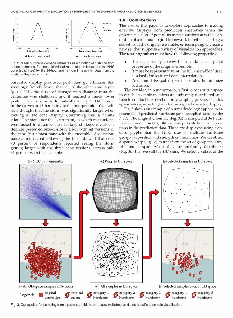
ensemble display produced peak damage estimates thatwere significantly lower than all of the other cone styles(p < 0:001), the curve of damage with distance from thecenterline was shallower, and it reached a much lowerpeak. This can be seen dramatically in Fig. 2. Differencesin the curves at 48 hours invite the interpretation that sub-jects thought that the storm was significantly larger whenlooking at the cone display. Confirming this, a “ThinkAloud” session after the experiment, in which respondentswere asked to describe their ranking strategy, revealed adefinite perceived size-of-storm effect with all versions ofthe cone, but almost none with the ensemble. A question-naire administered following the trials showed that circa70 percent of respondents reported seeing the stormgetting larger with the three cone versions, versus only31 percent with the ensemble.

1.4 Contributions

The goal of this paper is to explore approaches to makingeffective displays from prediction ensembles when theensemble is a set of points. Its main contribution is the elab-oration of a methodological framework for either selecting asubset from the original ensemble, or resampling to create anew set that supports a variety of visualization approaches.The resulting subset must have the following properties:

� It must correctly convey the key statistical spatialproperties of the original ensemble.

� It must be representative of the full ensemble if usedas a basis for scattered data interpolation.

� Points must be spatially well separated to minimizeocclusion.

The key idea, in our approach, is first to construct a spacein which ensemble members are uniformly distributed, andthen to conduct the selection or resampling processes in thisspace before projecting back to the original space for display.

Fig. 3 shows an example of our methodology applied to anensemble of predicted hurricane paths supplied to us by theNHC. The original ensemble (Fig. 3a) is sampled at 36 hoursinto the prediction (Fig. 3b) to show possible hurricane posi-tions in the prediction data. These are displayed using stan-dard glyphs that the NHC uses to indicate hurricanegeospatial position and strength on their maps. We constructa spatial warp (Fig. 3c) to transform the set of geospatial sam-ples into a space where they are uniformly distributed(Fig. 3d) that we call the UD space. We select a subset of the

Fig. 2. Mean hurricane damage estimates as a function of distance fromcenter centerline, for ensemble visualization (dotted lines), and the NHCcone (solid lines) for the 24-hour and 48-hour time points. Data from thestudy by Ruginski et al. [4].

Fig. 3. Our pipeline for sampling from a path ensemble to produce a well structured time-specific ensemble visualization.

LIU ET AL.: UNCERTAINTY VISUALIZATION BY REPRESENTATIVE SAMPLING FROM PREDICTION ENSEMBLES 2167

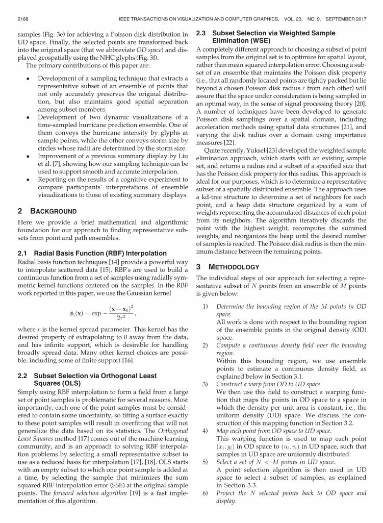
samples (Fig. 3e) for achieving a Poisson disk distribution inUD space. Finally, the selected points are transformed backinto the original space (that we abbreviate OD space) and dis-played geospatially using theNHCglyphs (Fig. 3f).

The primary contributions of this paper are:

� Development of a sampling technique that extracts arepresentative subset of an ensemble of points thatnot only accurately preserves the original distribu-tion, but also maintains good spatial separationamong subset members.

� Development of two dynamic visualizations of atime-sampled hurricane prediction ensemble. One ofthem conveys the hurricane intensity by glyphs atsample points, while the other conveys storm size bycircles whose radii are determined by the storm size.

� Improvement of a previous summary display by Liuet al. [7], showing how our sampling technique can beused to support smooth and accurate interpolation.

� Reporting on the results of a cognitive experiment tocompare participants’ interpretations of ensemblevisualizations to those of existing summary displays.

2 BACKGROUND

Here we provide a brief mathematical and algorithmicfoundation for our approach to finding representative sub-sets from point and path ensembles.

2.1 Radial Basis Function (RBF) Interpolation

Radial basis function techniques [14] provide a powerful wayto interpolate scattered data [15]. RBF’s are used to build acontinuous function from a set of samples using radially sym-metric kernel functions centered on the samples. In the RBFwork reported in this paper, we use the Gaussian kernel

fiðxÞ ¼ exp� ðx� x0Þ22r2

;

where r is the kernel spread parameter. This kernel has thedesired property of extrapolating to 0 away from the data,and has infinite support, which is desirable for handlingbroadly spread data. Many other kernel choices are possi-ble, including some of finite support [16].

2.2 Subset Selection via Orthogonal LeastSquares (OLS)

Simply using RBF interpolation to form a field from a largeset of point samples is problematic for several reasons. Mostimportantly, each one of the point samples must be consid-ered to contain some uncertainty, so fitting a surface exactlyto these point samples will result in overfitting that will notgeneralize the data based on its statistics. The OrthogonalLeast Squaresmethod [17] comes out of the machine learningcommunity, and is an approach to solving RBF interpola-tion problems by selecting a small representative subset touse as a reduced basis for interpolation [17], [18]. OLS startswith an empty subset to which one point sample is added ata time, by selecting the sample that minimizes the sumsquared RBF interpolation error (SSE) at the original samplepoints. The forward selection algorithm [19] is a fast imple-mentation of this algorithm.

2.3 Subset Selection via Weighted SampleElimination (WSE)

A completely different approach to choosing a subset of pointsamples from the original set is to optimize for spatial layout,rather thanmean squared interpolation error. Choosing a sub-set of an ensemble that maintains the Poisson disk property(i.e., that all randomly located points are tightly packed but liebeyond a chosen Poisson disk radius r from each other) willassure that the space under consideration is being sampled inan optimal way, in the sense of signal processing theory [20].A number of techniques have been developed to generatePoisson disk samplings over a spatial domain, includingacceleration methods using spatial data structures [21], andvarying the disk radius over a domain using importancemeasures [22].

Quite recently, Yuksel [23] developed theweighted sampleelimination approach, which starts with an existing sampleset, and returns a radius and a subset of a specified size thathas the Poisson disk property for this radius. This approach isideal for our purposes, which is to determine a representativesubset of a spatially distributed ensemble. The approach usesa kd-tree structure to determine a set of neighbors for eachpoint, and a heap data structure organized by a sum ofweights representing the accumulated distances of each pointfrom its neighbors. The algorithm iteratively discards thepoint with the highest weight, recomputes the summedweights, and reorganizes the heap until the desired numberof samples is reached. The Poisson disk radius is then themin-imumdistance between the remaining points.

3 METHODOLOGY

The individual steps of our approach for selecting a repre-sentative subset of N points from an ensemble of M pointsis given below:

1) Determine the bounding region of the M points in ODspace.All work is done with respect to the bounding regionof the ensemble points in the original density (OD)space.

2) Compute a continuous density field over the boundingregion.Within this bounding region, we use ensemblepoints to estimate a continuous density field, asexplained below in Section 3.1.

3) Construct a warp from OD to UD space.We then use this field to construct a warping func-tion that maps the points in OD space to a space inwhich the density per unit area is constant, i.e., theuniform density (UD) space. We discuss the con-struction of this mapping function in Section 3.2.

4) Map each point from OD space to UD space.This warping function is used to map each pointðxi; yiÞ in OD space to ðui; viÞ in UD space, such thatsamples in UD space are uniformly distributed.

5) Select a set of N < M points in UD space.A point selection algorithm is then used in UDspace to select a subset of samples, as explainedin Section 3.3.

6) Project the N selected points back to OD space anddisplay.


Finally, the selected points in UD space are mappedback to OD space for display, as discussed in Section3.4.

As long as the selected subset is uniformly distributed inUD space, we have a guarantee that the corresponding sam-ple set in OD space is representative of the statistical prop-erties of the original ensemble. Note, that this approach isinsensitive to whether or not the original distribution isunimodal or multimodal. In either case, the distribution weend up with in UD space is uniform, while the inverse mapback to OD space restores the original modality.

3.1 Computing the Continuous Density Field

We compute the density field over the sample space usingradial basis function interpolation, after assigning a localdata density value to each sample point. We avoid using agrid-based discretization for the density estimation, becausethe input data from the original ensemble may be distrib-uted in a highly non-uniform way, which can lead to sam-pling issues. Instead, we directly use the samples of theoriginal ensemble utilizing a k nearest neighbors (kNN)approach [24].

Given a sample point i with position xi ¼ ðxi; yiÞ, from adata set of sizeM, the kNNdensity si at this point is defined as

si ¼ k

Mpri2;

where ri is the radius of the circle with center at xi that min-imally encloses the k nearest neighbors of the point i. A kd-tree can be used for rapid determination of the k nearestneighbors of each sample point.

However, interpolating the density field from all of thepoints in the ensemble would result in overfitting. There-fore, we use the forward selection implementation of theOLS algorithm [19] to select a subset that minimizes meansquared interpolation error. For each sample point i wecompute an RBF spread parameter

ri ¼ bwffiffiffiffiffisi

p ; (1)

that adapts to the local density measure. Here,w is the largestdimension of the bounding region in OD space, and b is auser settable constant. In this way, the RBF interpolation algo-rithm can handle scattered datawithwidely varying density.

It is possible to use the subset of the original pointsobtained with this procedure as the subset for displayingthe ensemble as well. However, by design, this subset ismore uniformly distributed than the original data set.Therefore, it does not provide a good representation of thestatistical properties of the original ensemble. Furthermore,this subset can also contain points that are too closetogether, resulting in glyph occlusion. These two problemscan be clearly seen in Fig. 4. Comparing the original ensem-ble of time-specific hurricane position predictions (Fig. 4a)to the subset of 100 sample points chosen by the OLS algo-rithm (Fig. 4b), it is apparent that the resulting subset is toouniform and some points are too close together. These arelimitations of not only the OLS approach, but any samplingalgorithm selecting a subset of points in the space they areoriginally living in. To address these limitations, we per-form our sample selection in UD space.

3.2 Mapping from OD to UD Space

There are a number of ways to construct a mapping

OD;UD � R2; f : UD ! OD; ðx; yÞ7!ðu; vÞ;

but not all of these result in a warp suited to our purposes.Our warp function shouldminimize both shear and non-uni-form scaling, since the selection process in UD space will bebased on euclidean distances between the points. Locally, themapping should be as close as possible to uniform scaling.

It is possible to define a mapping from a non-uniformdistribution to a uniform distribution using a cumulativedensity function. In R2, the probability density p at positionðx; yÞ can be written as

pðx; yÞ ¼ pxðxÞpyðyjxÞ;where

pxðxÞ ¼Z y

�1pðx; yÞdy and pyðyjxÞ ¼ pðx; yÞ=pxðxÞ;

yielding

uðx; yÞ ¼Z x

�1pxðxÞdx; and vðx; yÞ ¼

Z y

�1pyðyjxÞdy:

Although this mapping results in a uniform distribution, itintroduces a great deal of shear along the v axis, such thatpoints that are distant from each other in OD space can bemoved near to each other in UD space, and vice versa.Therefore, the Euclidian distances between points in UDspace will not be a good metric for selecting a subset.

The approach that we have found to be most useful is aGauss-Seidel style relaxation process. We begin with splittingthe OD space into a number of grid cells with uniform sizes.In UD space, this grid should be deformed, such that the areaof each grid cell should roughly correspond to the densitywithin the grid cell in OD space. The deformation of this gridrepresents our warping function. A point ðxi; yiÞ in a grid cellin OD space is mapped to ðui; viÞ in the corresponding cell inUD space, usingmatching barycentric coordinates.

3.2.1 Relaxation for Grid-Based Warping Function

Without loss of generality, let us assume that the initial gridis a square with dimensions S � S. Since UD space has uni-form density, each deformed grid cell in UD space shouldhave the same average density

Fig. 4. An optimal subset chosen using OLS in the original space, is toouniformly distributed.


da ¼PS2

j¼1 dj

S2A;

where dj is the initial density of the cell j and A is the initialarea of a grid cell. In practice, we estimate the initial densitydj of a grid cell by sampling at the center of the cell, usingthe kNN density field described in Section 3.1. The targetarea of a cell Aj can be written as

Aj ¼ Adjda

:

For computing the deformed grid, we assign a target lengthto each edge of the grid using the Aj values of the neighbor-ing cells. The target length of an edge k on the perimeter ofthe grid that has a single cell neighbor j is

Lk ¼ L

ffiffiffiffiffiffiAj

A

r;

where L is the initial length of a grid edge. For other edgesthat are shared between two cells, we use the average of thetwo target length values computed for each face. We alsoconstruct two diagonal edges for each cell to minimize shearduring the relaxation. The target lengths of the diagonaledges are computed similarly, using the target areas of theircells. The structure of a single cell is shown in Fig. 5a.

Our relaxation process changes the length of each edge ktowards the target length Lk, at each step t, by moving itsvertices along the edge direction. Let pt

i and ptiþ1 be the posi-

tions of the two vertices of an edge k at relaxation step t, as

shown in Fig. 5b. The updated position of the vertex ptþ1i

due to the update operation for edge k can be written as

ptþ1i ¼ pt

i þ aLtk � Lk

2

� �ptiþ1 � pt

i

Ltk

� �; (2)

where Ltk ¼ pt

iþ1 � pti

�� is the length of the edge at relaxationstep t and 0 < a � 1 is a user adjustable acceleration factor,

such that if a ¼ 1, Ltþ1k ¼ Lk at the end of the update for

edge k.

3.2.2 Hierarchical Relaxation

For achieving a high quality warping function, we need tohave a high-resolution grid. But, when the displacement ofthe grid vertices due to the deformation of the grid is muchlarger than the length of a grid edge, the relaxation processcan result in crossed edges, inverting cells and thus chang-ing the grid’s topology, leading to instability. To avoid this,we use a hierarchical progressive-refinement approach, asillustrated in Fig. 6. We first use relaxation to compute alow-resolution deformed grid. Then, we subdivide the cellsand continue the relaxation process for the subdivided grid

with higher resolution. This way, large deformations of thegrid are handled using lower resolution grids and finedetails of the deformation are introduced using relaxationof higher resolution grids.

The relaxation process that we use to obtain a solution ata level in the hierarchy has two stopping conditions. First,we monitor the sum of squared errors (SSE), defined as thesum of squared differences between desired areas and cur-rent areas of all grid cells

SSE ¼XS2kp¼1

ðADp �ApÞ2;

where Sk denotes the grid dimension at the kth level in thehierarchy. We terminate the relaxation if the SSE is less thana small threshold. The second stopping condition is thedetection of an inverted cell. When a target cell area is verysmall, the relaxation process can still produce inversion. If aninverted cell is detected, we restore the system to its previousstate and terminate the relaxation for that level of the hierar-chy and continue the relaxation at the next lower level.

At each stage of the refinement process, we try to adjustthe area of each grid cell so that its density equals the aver-age density of the OD domain. In our implementation, weset the grid dimensions as powers of two, so we associatethe finest grid dimensions S � S withM samples using

S ¼ blog2 gMc; (3)

where g is a user adjustable fraction between 0 and 1. If S0 isthe dimension of the grid at the coarsest level, our methodrequires

T ¼ 1þ log2 S � log2 S0 (4)

hierarchical levels to compute the highest resolutiondeformed grid.

3.3 Selecting a Representative Subset

In order to select a representative subset, we first transform allsamples in OD space to UD space. Subsequently, we choose arepresentative subset of the samples in UD space using eitherthe Orthogonal Least Squares algorithm explained in Section2.2 or the Weighted Sample Elimination method presented inSection 2.3. These two methods select subsets with differentfeatures.

The OLS method is a selection approach based on a con-struction of an RBF system. To avoid the high computa-tional cost of the naive OLS algorithm, we utilize Orr’sforward selection algorithm [19], which monitors the reduc-tion in SSE of the RBF system, aimed at selecting the mini-mal subset satisfying a specific error criterion. Whilebuilding the RBF, the righthand side of the linear system isassigned by computing simplicial depth values [25] of the

Fig. 5. Model used for a grid cell and its edges.

Fig. 6. Initial, and three levels of hierarchical refinement for computingthe warping function.


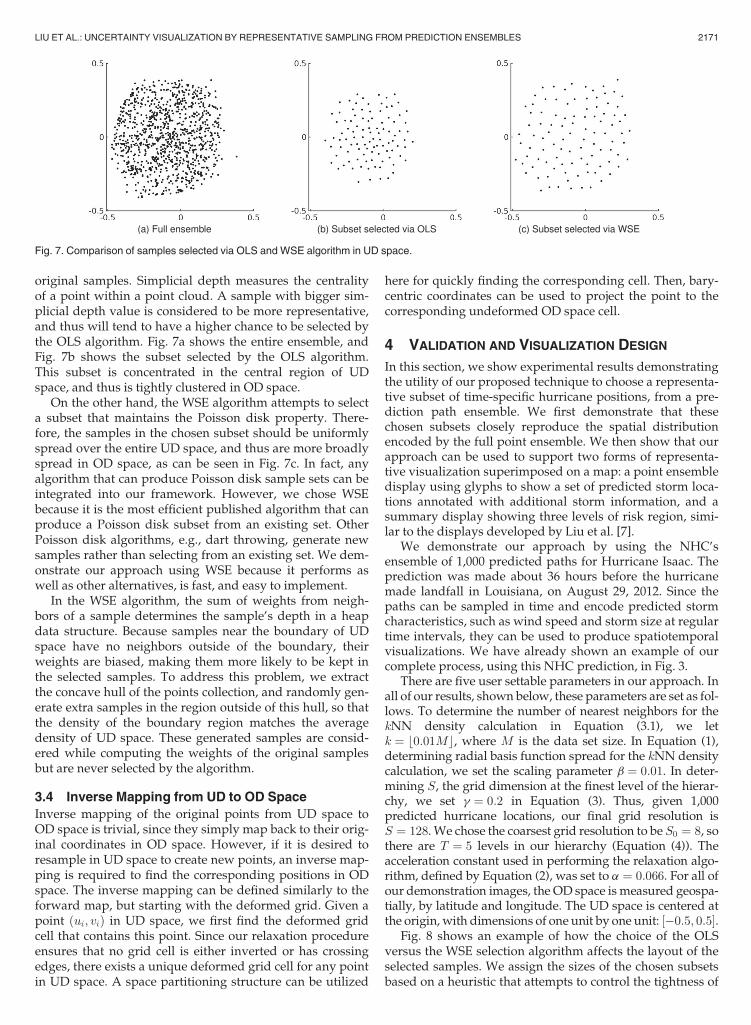
original samples. Simplicial depth measures the centralityof a point within a point cloud. A sample with bigger sim-plicial depth value is considered to be more representative,and thus will tend to have a higher chance to be selected bythe OLS algorithm. Fig. 7a shows the entire ensemble, andFig. 7b shows the subset selected by the OLS algorithm.This subset is concentrated in the central region of UDspace, and thus is tightly clustered in OD space.

On the other hand, the WSE algorithm attempts to selecta subset that maintains the Poisson disk property. There-fore, the samples in the chosen subset should be uniformlyspread over the entire UD space, and thus are more broadlyspread in OD space, as can be seen in Fig. 7c. In fact, anyalgorithm that can produce Poisson disk sample sets can beintegrated into our framework. However, we chose WSEbecause it is the most efficient published algorithm that canproduce a Poisson disk subset from an existing set. OtherPoisson disk algorithms, e.g., dart throwing, generate newsamples rather than selecting from an existing set. We dem-onstrate our approach using WSE because it performs aswell as other alternatives, is fast, and easy to implement.

In the WSE algorithm, the sum of weights from neigh-bors of a sample determines the sample’s depth in a heapdata structure. Because samples near the boundary of UDspace have no neighbors outside of the boundary, theirweights are biased, making them more likely to be kept inthe selected samples. To address this problem, we extractthe concave hull of the points collection, and randomly gen-erate extra samples in the region outside of this hull, so thatthe density of the boundary region matches the averagedensity of UD space. These generated samples are consid-ered while computing the weights of the original samplesbut are never selected by the algorithm.

3.4 Inverse Mapping from UD to OD Space

Inverse mapping of the original points from UD space toOD space is trivial, since they simply map back to their orig-inal coordinates in OD space. However, if it is desired toresample in UD space to create new points, an inverse map-ping is required to find the corresponding positions in ODspace. The inverse mapping can be defined similarly to theforward map, but starting with the deformed grid. Given apoint ðui; viÞ in UD space, we first find the deformed gridcell that contains this point. Since our relaxation procedureensures that no grid cell is either inverted or has crossingedges, there exists a unique deformed grid cell for any pointin UD space. A space partitioning structure can be utilized

here for quickly finding the corresponding cell. Then, bary-centric coordinates can be used to project the point to thecorresponding undeformed OD space cell.

4 VALIDATION AND VISUALIZATION DESIGN

In this section, we show experimental results demonstratingthe utility of our proposed technique to choose a representa-tive subset of time-specific hurricane positions, from a pre-diction path ensemble. We first demonstrate that thesechosen subsets closely reproduce the spatial distributionencoded by the full point ensemble. We then show that ourapproach can be used to support two forms of representa-tive visualization superimposed on a map: a point ensembledisplay using glyphs to show a set of predicted storm loca-tions annotated with additional storm information, and asummary display showing three levels of risk region, simi-lar to the displays developed by Liu et al. [7].

We demonstrate our approach by using the NHC’sensemble of 1,000 predicted paths for Hurricane Isaac. Theprediction was made about 36 hours before the hurricanemade landfall in Louisiana, on August 29, 2012. Since thepaths can be sampled in time and encode predicted stormcharacteristics, such as wind speed and storm size at regulartime intervals, they can be used to produce spatiotemporalvisualizations. We have already shown an example of ourcomplete process, using this NHC prediction, in Fig. 3.

There are five user settable parameters in our approach. Inall of our results, shown below, these parameters are set as fol-lows. To determine the number of nearest neighbors for thekNN density calculation in Equation (3.1), we letk ¼ b0:01Mc, where M is the data set size. In Equation (1),determining radial basis function spread for the kNN densitycalculation, we set the scaling parameter b ¼ 0:01. In deter-mining S, the grid dimension at the finest level of the hierar-chy, we set g ¼ 0:2 in Equation (3). Thus, given 1,000predicted hurricane locations, our final grid resolution isS ¼ 128. We chose the coarsest grid resolution to be S0 ¼ 8, sothere are T ¼ 5 levels in our hierarchy (Equation (4)). Theacceleration constant used in performing the relaxation algo-rithm, defined by Equation (2), was set to a ¼ 0:066. For all ofour demonstration images, the OD space ismeasured geospa-tially, by latitude and longitude. The UD space is centered atthe origin, with dimensions of one unit by one unit: ½�0:5; 0:5�.

Fig. 8 shows an example of how the choice of the OLSversus the WSE selection algorithm affects the layout of theselected samples. We assign the sizes of the chosen subsetsbased on a heuristic that attempts to control the tightness of

Fig. 7. Comparison of samples selected via OLS and WSE algorithm in UD space.


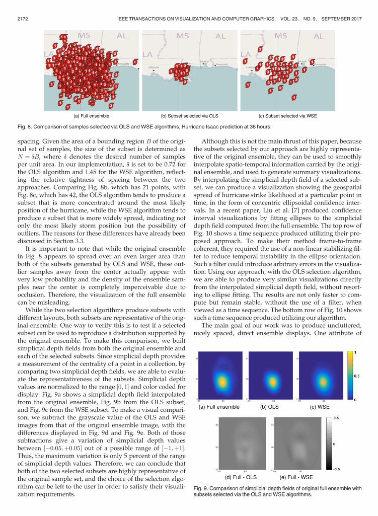
spacing. Given the area of a bounding region B of the origi-nal set of samples, the size of the subset is determined asN ¼ dB, where d denotes the desired number of samplesper unit area. In our implementation, d is set to be 0.72 forthe OLS algorithm and 1.45 for the WSE algorithm, reflect-ing the relative tightness of spacing between the twoapproaches. Comparing Fig. 8b, which has 21 points, withFig. 8c, which has 42, the OLS algorithm tends to produce asubset that is more concentrated around the most likelyposition of the hurricane, while the WSE algorithm tends toproduce a subset that is more widely spread, indicating notonly the most likely storm position but the possibility ofoutliers. The reasons for these differences have already beendiscussed in Section 3.3.

It is important to note that while the original ensemblein Fig. 8 appears to spread over an even larger area thanboth of the subsets generated by OLS and WSE, these out-lier samples away from the center actually appear withvery low probability and the density of the ensemble sam-ples near the center is completely imperceivable due toocclusion. Therefore, the visualization of the full ensemblecan be misleading.

While the two selection algorithms produce subsets withdifferent layouts, both subsets are representative of the orig-inal ensemble. One way to verify this is to test if a selectedsubset can be used to reproduce a distribution supported bythe original ensemble. To make this comparison, we builtsimplicial depth fields from both the original ensemble andeach of the selected subsets. Since simplicial depth providesa measurement of the centrality of a point in a collection, bycomparing two simplicial depth fields, we are able to evalu-ate the representativeness of the subsets. Simplicial depthvalues are normalized to the range ½0; 1� and color coded fordisplay. Fig. 9a shows a simplicial depth field interpolatedfrom the original ensemble, Fig. 9b from the OLS subset,and Fig. 9c from the WSE subset. To make a visual compari-son, we subtract the grayscale value of the OLS and WSEimages from that of the original ensemble image, with thedifferences displayed in Fig. 9d and Fig. 9e. Both of thosesubtractions give a variation of simplicial depth valuesbetween ½�0:05;þ0:05� out of a possible range of ½�1;þ1�.Thus, the maximum variation is only 5 percent of the rangeof simplicial depth values. Therefore, we can conclude thatboth of the two selected subsets are highly representative ofthe original sample set, and the choice of the selection algo-rithm can be left to the user in order to satisfy their visuali-zation requirements.

Although this is not the main thrust of this paper, becausethe subsets selected by our approach are highly representa-tive of the original ensemble, they can be used to smoothlyinterpolate spatio-temporal information carried by the origi-nal ensemble, and used to generate summary visualizations.By interpolating the simplicial depth field of a selected sub-set, we can produce a visualization showing the geospatialspread of hurricane strike likelihood at a particular point intime, in the form of concentric ellipsoidal confidence inter-vals. In a recent paper, Liu et al. [7] produced confidenceinterval visualizations by fitting ellipses to the simplicialdepth field computed from the full ensemble. The top row ofFig. 10 shows a time sequence produced utilizing their pro-posed approach. To make their method frame-to-framecoherent, they required the use of a non-linear stabilizing fil-ter to reduce temporal instability in the ellipse orientation.Such a filter could introduce arbitrary errors in the visualiza-tion. Using our approach, with the OLS selection algorithm,we are able to produce very similar visualizations directlyfrom the interpolated simplicial depth field, without resort-ing to ellipse fitting. The results are not only faster to com-pute but remain stable, without the use of a filter, whenviewed as a time sequence. The bottom row of Fig. 10 showssuch a time sequence produced utilizing our algorithm.

The main goal of our work was to produce uncluttered,nicely spaced, direct ensemble displays. One attribute of

Fig. 8. Comparison of samples selected via OLS and WSE algorithms, Hurricane Isaac prediction at 36 hours.

Fig. 9. Comparison of simplicial depth fields of original full ensemble withsubsets selected via the OLS and WSE algorithms.


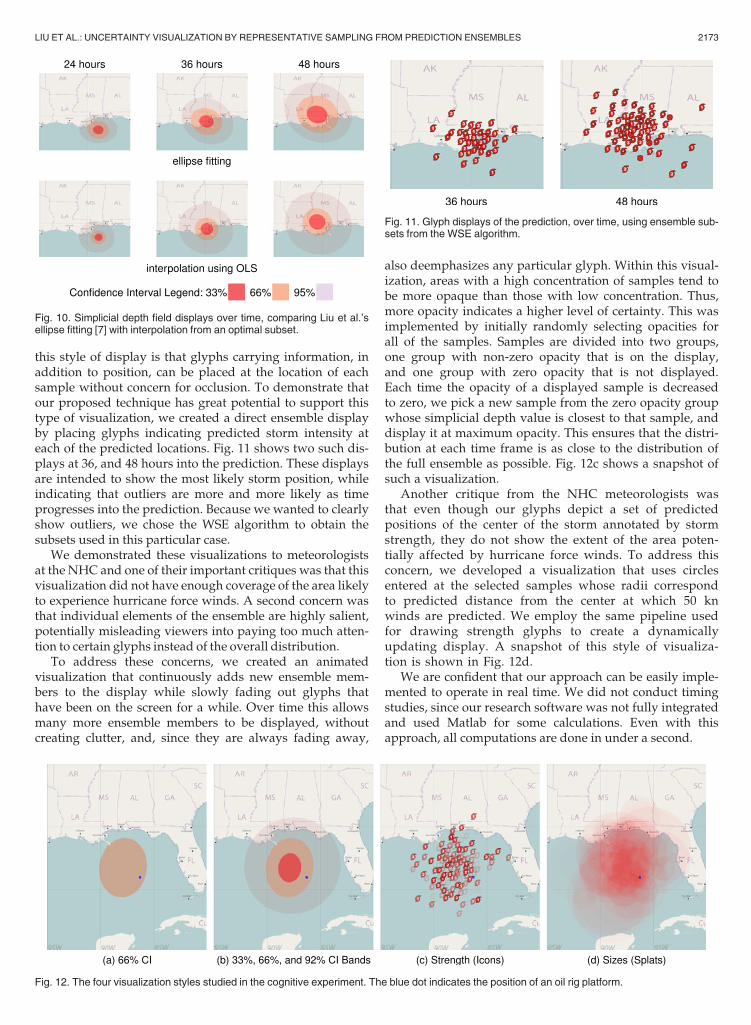
this style of display is that glyphs carrying information, inaddition to position, can be placed at the location of eachsample without concern for occlusion. To demonstrate thatour proposed technique has great potential to support thistype of visualization, we created a direct ensemble displayby placing glyphs indicating predicted storm intensity ateach of the predicted locations. Fig. 11 shows two such dis-plays at 36, and 48 hours into the prediction. These displaysare intended to show the most likely storm position, whileindicating that outliers are more and more likely as timeprogresses into the prediction. Because we wanted to clearlyshow outliers, we chose the WSE algorithm to obtain thesubsets used in this particular case.

We demonstrated these visualizations to meteorologistsat the NHC and one of their important critiques was that thisvisualization did not have enough coverage of the area likelyto experience hurricane force winds. A second concern wasthat individual elements of the ensemble are highly salient,potentially misleading viewers into paying too much atten-tion to certain glyphs instead of the overall distribution.

To address these concerns, we created an animatedvisualization that continuously adds new ensemble mem-bers to the display while slowly fading out glyphs thathave been on the screen for a while. Over time this allowsmany more ensemble members to be displayed, withoutcreating clutter, and, since they are always fading away,

also deemphasizes any particular glyph. Within this visual-ization, areas with a high concentration of samples tend tobe more opaque than those with low concentration. Thus,more opacity indicates a higher level of certainty. This wasimplemented by initially randomly selecting opacities forall of the samples. Samples are divided into two groups,one group with non-zero opacity that is on the display,and one group with zero opacity that is not displayed.Each time the opacity of a displayed sample is decreasedto zero, we pick a new sample from the zero opacity groupwhose simplicial depth value is closest to that sample, anddisplay it at maximum opacity. This ensures that the distri-bution at each time frame is as close to the distribution ofthe full ensemble as possible. Fig. 12c shows a snapshot ofsuch a visualization.

Another critique from the NHC meteorologists wasthat even though our glyphs depict a set of predictedpositions of the center of the storm annotated by stormstrength, they do not show the extent of the area poten-tially affected by hurricane force winds. To address thisconcern, we developed a visualization that uses circlesentered at the selected samples whose radii correspondto predicted distance from the center at which 50 knwinds are predicted. We employ the same pipeline usedfor drawing strength glyphs to create a dynamicallyupdating display. A snapshot of this style of visualiza-tion is shown in Fig. 12d.

We are confident that our approach can be easily imple-mented to operate in real time. We did not conduct timingstudies, since our research software was not fully integratedand used Matlab for some calculations. Even with thisapproach, all computations are done in under a second.

Fig. 10. Simplicial depth field displays over time, comparing Liu et al.’sellipse fitting [7] with interpolation from an optimal subset.

Fig. 11. Glyph displays of the prediction, over time, using ensemble sub-sets from the WSE algorithm.

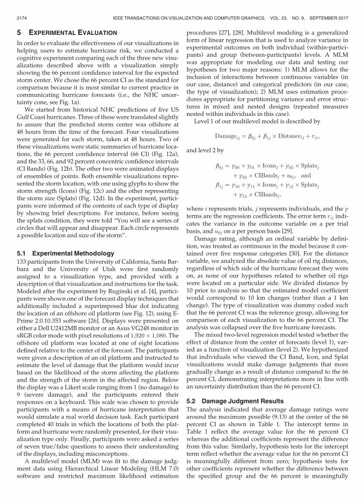
Fig. 12. The four visualization styles studied in the cognitive experiment. The blue dot indicates the position of an oil rig platform.


5 EXPERIMENTAL EVALUATION

In order to evaluate the effectiveness of our visualizations inhelping users to estimate hurricane risk, we conducted acognitive experiment comparing each of the three new visu-alizations described above with a visualization simplyshowing the 66 percent confidence interval for the expectedstorm center. We chose the 66 percent CI as the standard forcomparison because it is most similar to current practice incommunicating hurricane forecasts (i.e., the NHC uncer-tainty cone, see Fig. 1a).

We started from historical NHC predictions of five USGulf Coast hurricanes. Three of thesewere translated slightlyto assure that the predicted storm center was offshore at48 hours from the time of the forecast. Four visualizationswere generated for each storm, taken at 48 hours. Two ofthese visualizations were static summaries of hurricane loca-tions, the 66 percent confidence interval (66 CI) (Fig. 12a),and the 33, 66, and 92 percent concentric confidence intervals(CI Bands) (Fig. 12b). The other two were animated displaysof ensembles of points. Both ensemble visualizations repre-sented the storm location, with one using glyphs to show thestorm strength (Icons) (Fig. 12c) and the other representingthe storm size (Splats) (Fig. 12d). In the experiment, partici-pants were informed of the contents of each type of displayby showing brief descriptions. For instance, before seeingthe splats condition, they were told “You will see a series ofcircles that will appear and disappear. Each circle representsa possible location and size of the storm”.

5.1 Experimental Methodology

133 participants from the University of California, Santa Bar-bara and the University of Utah were first randomlyassigned to a visualization type, and provided with adescription of that visualization and instructions for the task.Modeled after the experiment by Ruginski et al. [4], partici-pants were shown one of the forecast display techniques thatadditionally included a superimposed blue dot indicatingthe location of an offshore oil platform (see Fig. 12), using E-Prime 2.0.10.353 software [26]. Displays were presented oneither a Dell U2412MBmonitor or an Asus VG248monitor insRGB color mode with pixel resolutions of 1;920� 1;080. Theoffshore oil platform was located at one of eight locationsdefined relative to the center of the forecast. The participantswere given a description of an oil platform and instructed toestimate the level of damage that the platform would incurbased on the likelihood of the storm affecting the platformand the strength of the storm in the affected region. Belowthe display was a Likert scale ranging from 1 (no damage) to9 (severe damage), and the participants entered theirresponses on a keyboard. This scale was chosen to provideparticipants with a means of hurricane interpretation thatwould simulate a real world decision task. Each participantcompleted 40 trials in which the locations of both the plat-form and hurricane were randomly presented, for their visu-alization type only. Finally, participants were asked a seriesof seven true/false questions to assess their understandingof the displays, includingmisconceptions.

A multilevel model (MLM) was fit to the damage judg-ment data using Hierarchical Linear Modeling (HLM 7.0)software and restricted maximum likelihood estimation

procedures [27], [28]. Multilevel modeling is a generalizedform of linear regression that is used to analyze variance inexperimental outcomes on both individual (within-partici-pants) and group (between-participants) levels. A MLMwas appropriate for modeling our data and testing ourhypotheses for two major reasons: 1) MLM allows for theinclusion of interactions between continuous variables (inour case, distance) and categorical predictors (in our case,the type of visualization); 2) MLM uses estimation proce-dures appropriate for partitioning variance and error struc-tures in mixed and nested designs (repeated measuresnested within individuals in this case).

Level 1 of our multilevel model is described by

Damageij ¼ b0j þ b1j �Distanceij þ rij;

and level 2 by

b0j ¼ g00 þ g01 � Iconsj þ g02 � Splatsj

þ g03 � CIBandsj þ u0j; and

b1j ¼ g10 þ g11 � Iconsj þ g12 � Splatsj

þ g13 � CIBandsj;

where i represents trials, j represents individuals, and the gterms are the regression coefficients. The error term rij indi-cates the variance in the outcome variable on a per trialbasis, and u0j on a per person basis [29].

Damage rating, although an ordinal variable by defini-tion, was treated as continuous in the model because it con-tained over five response categories [30]. For the distancevariable, we analyzed the absolute value of oil rig distances,regardless of which side of the hurricane forecast they wereon, as none of our hypotheses related to whether oil rigswere located on a particular side. We divided distance by10 prior to analysis so that the estimated model coefficientwould correspond to 10 km changes (rather than a 1 kmchange). The type of visualization was dummy coded suchthat the 66 percent CI was the reference group, allowing forcomparison of each visualization to the 66 percent CI. Theanalysis was collapsed over the five hurricane forecasts.

The mixed two-level regression model tested whether theeffect of distance from the center of forecasts (level 1), var-ied as a function of visualization (level 2). We hypothesizedthat individuals who viewed the CI Band, Icon, and Splatvisualizations would make damage judgments that moregradually change as a result of distance compared to the 66percent CI, demonstrating interpretations more in line withan uncertainty distribution than the 66 percent CI.

5.2 Damage Judgment Results

The analysis indicated that average damage ratings werearound the maximum possible (9.13) at the center of the 66percent CI as shown in Table 1. The intercept terms inTable 1 reflect the average value for the 66 percent CIwhereas the additional coefficients represent the differencefrom this value. Similarly, hypothesis tests for the interceptterm reflect whether the average value for the 66 percent CIis meaningfully different from zero; hypothesis tests forother coefficients represent whether the difference betweenthe specified group and the 66 percent is meaningfully


different from zero. The average damage rating value is esti-mated above the top of the scale since individuals nevermade a damage judgment exactly at the center of the hurri-cane. Compared to the 66 percent CI, damage judgmentsmade using the CI Bands at the center of the hurricane fore-cast were 1.43 lower on average, and judgments made usingthe Icon were 2.53 lower on average. Interestingly, averagedamage ratings made at the center of the forecast using theSplat visualization were not meaningfully different fromthose made using the 66 percent CI.

Second, our analysis revealed a significant associationbetween distance and damage rating for the 66 percent CIvisualization. There was a 0.21 decrease in damage judg-ment per 10 km on average as shown in Table 2. This wasexpected, given that individuals had little information asidefrom distance when making damage judgments using thisvisualization. More importantly, both the CI Bands visuali-zation (0.157 decrease per 10 km, see Fig. 13a) and the Iconvisualization (0.116 decrease per 10 km, see Fig. 13b) dem-onstrated a significantly less strong association between dis-tance and damage rating than the 66 percent CI. Lastly, therelationship between distance-from-center and damage rat-ing for the Splats visualization did not differ significantlyfrom the 66 percent CI visualization (see Fig. 13c).

5.3 Post-task Questionnaire Results

In a post-task survey, participants were asked a series ofseven true/false questions (given in Table 3). We com-pared each of the other visualization conditions to the 66percent CI condition using chi-squared tests ofindependence.

Responses to Questions 2, 3, and 4 did not differ signifi-cantly, indicating that across all conditions, most partici-pants understood that the displays indicate 1) that the areabeing shown has a chance of being damaged, 2) where thecenter of the storm is likely to be, and 3) that the forecastersare uncertain of the storm’s location.

Responses to Question 1 indicated that participants in theCI Bands group, x2ð1; N ¼ 65Þ ¼ 4:99; p ¼ 0:03, and partici-

pants in the Splats condition, x2ð1; N ¼ 62Þ ¼ 10:09; p ¼0:001, were more likely to endorse the statement that theforecast shows a distribution of possible locations.

Importantly, although only the Splats condition showedthe size of the hurricane, there was no significant differencebetween conditions in endorsement of Statement 5 that theforecast visualization indicates the size of the hurricane.Participants in the 66 percent CI condition in particular, hadvery similar endorsement rates of this statement to partici-pants in the Splats condition, indicating a strong misconcep-tion that size of glyph indicates size of hurricane.

There does not seem to be strong misconception that thesize of the glyph in the 66 percent CI condition indicates inten-sity (see responses to Statement 6). Optimistically, most par-ticipants in the Icon display condition correctly indicated thatthis display showed intensity and were significantly differentfrom the 66 percent CI condition, x2ð1; N ¼ 62Þ ¼ 47:23;

p < 0:001. However the CI Bands condition, x2ð1;N ¼ 65Þ ¼10:11; p ¼ 0:001, and the Splats condition, x2ð1;N ¼ 62Þ ¼25:06; p < 0:001, were also more likely (than the 66 percentconfidence interval group) to endorse the statement that thedisplays showed intensity of the hurricane, although neitherof these displays actually shows intensity.

Finally, although none of these displays shows the passageof time, participants in the two animation conditions (Splats,

x2ð1;N ¼ 62Þ ¼ 16:93; p < :001; Icon, x2ð1; N ¼ 62Þ ¼ 16:93;p < 0:001) weremore likely to endorse Statement 7 comparedto the 66 percent CI condition. This result suggests a possiblemisconception that change of time in a display indicateschange over time in the forecast.

5.4 Experiment Summary

Overall, our analysis revealed that the CI Bands and Icon visu-alizations were interpreted as changing more gradually as a

TABLE 1Intercept Level 1, b0

Fixed Effect Coeff. Std Err t-ratio DOF p-value 95% CI

Intercept 2, g00 9.129 0.177 51.68 119 < 0.001 (8.78,9.48)Icons, g01 �2.525 0.371 �6.79 119 < 0.001 (�3.26, �1.79)Splats, g02 0.159 0.221 0.72 119 0.473 (�0.27, 0.59)CI Bands, g03 �1.433 0.353 �4.06 119 < 0.001 (�2.12, �0.74)

Average damage judgments made at the center of the forecasts. Main effect(intercept) references 66 percent CI visualization. The Table summarizes thecomparison of each visualization to the 66 percent CI.

TABLE 2Slope Level 1, b1

Fixed Effect Coeff Std Err t-ratio DOF p-value 95% CI

Intercept 2, g10 �0.210 0.006 �32.36 4793 < 0.001 (�0.22,-0.19)

Icons, g11 0.094 0.015 6.31 4793 < 0.001 (0.06, 0.12)

Splats, g12 �0.003 0.009 �0.36 4793 0.720 (�0.02, 0.01)

CI Bands, g13 0.053 0.018 2.94 4793 0.003 (0.02, 0.09)

Effect of a 10 km change in distance on damage ratings. Main effect (intercept)references 66 percent CI visualization. The table summarizes the comparisonof each visualization to the 66 percent CI.

Fig. 13. Mean damage ratings as a function of distance from the center of the storm. Each visualization is compared to the 66 percent CI.


function of distance than the 66 percent CI visualization. Thissuggests that the former two were interpreted more like anuncertainty distribution than the 66 percent CI, and is similarto the effect seen with the path ensemble displays used in theearlier experiment by Ruginksi et al. [4]. However, the Splatsvisualization was interpreted similarly to the 66 percent CI,both in terms of average overall damage rating providedacross all trials and the change in damage ratings thatoccurred as a function of distance-from-center. Although theCI bands and Icon visualizations were interpreted as morelike an uncertainty visualization, and alleviated somemiscon-ceptions, answers to the questionnaire showed that othermis-conceptions about these displays remained. For example,many viewers saw the animated displays as indicating thepassage of time. An interesting and unexpected result wasthat, even though they were not visually similar, the 92 per-cent CI and Icon displays elicited remarkably similar judg-ments. This indicates that decisions are likely driven by thespatial properties, not just the ensemble or summary nature ofthe display, and suggests a direction for future study.

6 CONCLUSION

We first made the case that the direct display of an ensembleof predictions can be superior to a statistical summary dis-play for conveying the uncertainty in a prediction. Theproblem is that such displays can be cluttered and difficultto interpret if the original ensemble is too large. We thenpresented a sampling approach that extracts a representa-tive subset of an ensemble of points while maintaining thestatistical spatial distribution of the full ensemble, andshowed how such a subset can be used to construct anensemble-based visualization, supporting the superimposi-tion of additional information on each sample via glyphs.As a byproduct, we also showed how the subset can beused as a basis for interpolation to create nicely-structuredsummary displays.

We have demonstrated our approach using hurricanepredictions as an example, showing how our ensembleapproach can be used to make time-specific visualizationsof hurricane position, strength, and size. None of the cur-rently produced visualizations from the National HurricaneCenter are either time-specific, or able to simultaneouslyshow the distribution of multiple storm attributes.

Additionally, we conducted a cognitive experiment tocompare our ensemble visualizations to summary displaysby examining participants’ estimations of potential stormdamage. The results indicate that an ensemble display usingicons showing storm intensity, based on a representative

subset of samples, can be effective in helping users to morecorrectly estimate the risk-which inherently includes esti-mating both the likelihood of a storm hitting and the inten-sity of the storm. This result is consistent with earlierexperiments showing that ensemble displays are effectivein reducing confusion between uncertainty and storm size.

In choosing subsets of an ensemble to support our visual-izations, we explored both the OLS and WSE selection algo-rithms. These produce subsets with different spatialcharacteristics. OLS subsets are tightly distributed, with fewoutliers. WSE subsets, on the other hand, are less tightly dis-tributed and include some outliers. For the hurricane predic-tion visualization problem, the tight distribution of OLS isgood at showing the most likely location of the storm, and isuseful for supporting interpolation-based summary displays.The broader distribution ofWSE has the advantage ofmakingthe viewer aware of the high uncertainty in the prediction,and is most useful for supporting ensemble-based displays.For future work, we would like to explore a hybrid of the twoalgorithms, choosing a subset that emphasizes layout central-ity, while preserving heightened awareness of outliers.

While our subset selection method preserves spatial distri-bution, there is no guarantee that it preserves the distributionof ancillary information, such as storm strength and size. Weare examining approaches to preserving the distributions ofall information, while still supporting good spatial layout.

ACKNOWLEDGMENTS

The authors would like to thank Ricardo Gutierrez-Osuna ofTexas A&MUniversity, Edward Rappaport andMark DeMa-ria of the National Hurricane Center, and Matthew Green ofFEMA for key discussions and advice. The work reported inthis paper was supported in part by the US National ScienceFoundation under Grant Nos. IIS-1212501, IIS-1212577, andIIS-1212806.

REFERENCES

[1] K. Potter, P. Rosen, and C. R. Johnson, “From quantification tovisualization: A taxonomy of uncertainty visualization approach-es,” IFIP Adv. Inf. Commun. Technol. Series, 2012, pp. 226–249.

[2] D. Stephenson and F. Doblas-Reyes, “Statistical methods for inter-preting Monte Carlo ensemble forecasts,” Tellus, vol. 52A,pp. 300–322, 2000.

[3] A. Pang, “Visualizing uncertainty in natural hazards,” in RiskAssessment, Modeling and Decision Support, vol. 14. Berlin,Germany: Springer, 2008, pp. 261–294. [Online]. Available:http://dx.doi.org/10.1007/978–3-540-71158-2_12

[4] I. T. Ruginski, et al., “Non-expert interpretations of hurricane fore-cast uncertainty visualizations,” Spatial Cognition Comput., vol. 16,no. 2, pp. 154–172, 2016.

TABLE 3Percentage of Participants in Agreement (Out of Total Answering)

Statement 66% CI CI Bands Splats Icons

1) The forecast shows a distribution of possible hurricane locations 63.6% 87.5% 96.6% 82.8%2) The forecast shows the area that has a chance of being damaged 78.8% 87.5% 93.1% 92.9%3) The forecast shows where the center of the hurricane has a chance of being 87.9% 87.5% 93.1% 92.9%4) The forecast visualization indicates that the forecasters are not certain about the location 66.7% 68.8% 62.1% 44.8%5) The forecast visualization indicates the size of the hurricane 57.6% 40.6% 58.6% 37.9%6) The forecast visualization indicates the intensity of the hurricane 9.1 % 43.8% 71.4% 96.6%7) The forecast visualization indicates the passing of time 0.0 % 6.3 % 41.4% 41.4%

Roughly 1/3 of the respondents were in each visualization category.


[5] R. Whitaker, M. Mirzargar, and R. Kirby, “Contour boxplots: Amethod for characterizing uncertainty in feature sets from simula-tion ensembles,” IEEE Trans. Vis. Comput. Graph., vol. 19, no. 12,pp. 2713–2722, Dec. 2013.

[6] M. Mirzargar, R. Whitaker, and R. Kirby, “Curve boxplot: Gener-alization of boxplot for ensembles of curves,” IEEE Trans. Vis.Comput. Graph., vol. 20, no. 12, pp. 2654–2663, Dec. 2014.

[7] L. Liu, M. Mirzargar, R. Kirby, R. Whitaker, and D. House,“Visualizing time-specific hurricane predictions, with uncertainty,from storm path ensembles,” Comput. Graph. Forum, vol. 34, no. 3,pp. 371–380, 2015.

[8] N. H. C. NOAA, “Definition of the NHC track forecast cone,”Dec. 2014. [Online]. Available: http://www.nhc.noaa.gov/aboutcone.shtml

[9] K. Broad, A. Leiserowitz, J. Weinkle, and M. Steketee,“Misinterpretations of the “cone of uncertainty” in Florida duringthe 2004 hurricane season,” Bulletin Amer. Meteorological Soc.,vol. 88, no. 5, pp. 651–667, 2007.

[10] L. Gedminas, “Evaluating hurricane advisories using eye-trackingand biometric data,” Master’s thesis, Faculty Dept. Geography,East Carolina Univ., Greenville, NC, Jun. 2011.

[11] J. Cox, D. House, and M. Lindell, “Visualizing uncertainty in pre-dicted hurricane tracks,” Int. J. Uncertainty Quantification, vol. 3,no. 2, pp. 143–156, 2013.

[12] L.-Y. Wei, “Multi-class blue noise sampling,” in Proc. ACM SIG-GRAPH, 2010, pp. 79:1–79:8. [Online]. Available: http://doi.acm.org/10.1145/1833349.1778816

[13] H. Chen, et al., “Visual abstraction and exploration of multi-classscatterplots,” IEEE Trans. Vis. Comput. Graph., vol. 20, no. 12,pp. 1683–1692, Dec. 2014.

[14] D. S. Broomhead and D. Lowe, “Multivariable functional interpo-lation and adaptive networks,” Complex Syst., vol. 2, pp. 321–355,1988.

[15] J. C. Carr, et al., “Reconstruction and representation of 3d objectswith radial basis functions,” in Proc. 28th Annu. Conf. Comput.Graph. Interactive Techn., 2001, pp. 67–76.

[16] M. D. Buhman, Radial Basis Functions: Theory and Implementations.Cambridge, U.K.: Cambridge Univ. Press, 2004.

[17] S. Chen, C. Cowan, and P. Grant, “Orthogonal least squares learn-ing algorithm for radial basis function networks,” IEEE Trans.Neural Netw., vol. 2, no. 2, pp. 302–309, Mar. 1991.

[18] S. Chen, E. Chng, and K. Alkadhimi, “Regularized orthogonalleast squares algorithm for constructing radial basis functionnetworks,” Int. J. Control, vol. 64, no. 5, pp. 829–837, 1996.

[19] M. J. L. Orr, Introduction to Radial Basis Function Networks, 1996.[Online]. Available: http://www.anc.ed.ac.uk/rbf/papers/intro.ps, Accessed on: Feb. 2015.

[20] R. L. Cook, “Stochastic sampling in computer graphics,” ACMTrans. Graph., vol. 5, no. 1, pp. 51–72, Jan. 1986. [Online]. Avail-able: http://doi.acm.org/10.1145/7529.8927

[21] D. Dunbar and G. Humphreys, “A spatial data structure for fastPoisson-disk sample generation,” ACM Trans. Graph., vol. 25,no. 3, pp. 503–508, 2006.

[22] M. McCool and E. Fiume, “Hierarchical Poisson Disk samplingdistributions,” in Proc. Graph. Interface, 1992, pp. 94–105.

[23] C. Yuksel, “Sample elimination for generating Poisson disk sam-ple sets,” Comput. Graph. Forum, vol. 34, no. 2, pp. 25–32, 2015.

[24] E. Fix and J. Hodges, Discriminatory analysis, nonparametricdiscrimination: Consistency properties, U.S. Air Force SchoolAviation Medicine, Randolph Field, TX, USA, Project 21-49-004,Rep. 4, Feb. 1951.

[25] R. Y. Liu, “On a notion of data depth based on random simplices,”Ann. Statist., vol. 18, no. 1, pp. 405–414, 1990.

[26] W. Schneider, A. Eschman, and A. Zuccolotto, E-Prime user’s guide.Pittsburgh, Pa, USA: Psychology Softw. Tools, 2012.

[27] S. Raudenbush, Y. C. A.S. Bryk, R. Congdon, and M. du Toit, Hier-archical Linear Modeling 7. Lincolnwood, IL, USA: Scientific Softw.Int. Inc., 2011.

[28] S. Raudenbush and A. Bryk, Hierarchical Linear Models: Applica-tions and Data Analysis Methods, vol. 1. Newbury Park, CA, USA:Sage, 2002.

[29] J. Cohen, P. Cohen, S. G. West, and L. S. Aiken, Applied MultipleRegression/Correlation Analysis for the Behavioral Sciences. Evanston,IL, USA: Routledge, 2013.

[30] D. Bauer and S. Sterba, “Fitting multilevel models with ordinaloutcomes: Performance of alternative specifications and methodsof estimation,” Psychol Methods, vol. 16, pp. 373–90, 2011.

Le Liu received the BS degree in computer sci-ence from Chongqing University, and the MSdegree in computer science fromClemsonUniver-sity. He is working toward the PhD degree in theSchool of Computing, Clemson University. Hisresearch interests include visualization and com-puter graphics. He is currently working on devel-oping novel techniques for visualizing hurricaneforecasts from path prediction ensembles. He is astudent member of the IEEEComputer Society.

Alexander P. Boone received the BA degrees inpsychology and history from the University ofMissouri, in 2010. He is now working toward thePhD degree in the Department of Psychologicaland Brain Sciences, University of California,Santa Barbara. He is widely interested in individ-ual differences in spatial cognition of small andlarge scale phenomena, particularly where it con-cerns issues of human navigation.

Ian T. Ruginski received the BA degree in cogni-tive science and religious studies from VassarCollege and the MS degree in psychology fromthe University of Utah. He is currently workingtoward the PhD degree in the Department of Psy-chology, University of Utah, specializing in visualperception and spatial cognition. His researchinterests include applying cognitive theory touncertainty visualization design and evaluation,as well as the influence of emotional and socialfactors on perception and performance.

Lace Padilla is working toward the PhD degree inthe Cognitive Neural Science Department, Univer-sity of Utah. She is a member of the Visual Percep-tion Spatial Cognition Research Group directed bySarah Creem-Regehr, PhD, Jeanine Stefanucci,PhD, and William Thompson, PhD. Her workfocuses on graphical cognition, decision-makingwith visualizations, and visual perception. Sheworks on large interdisciplinary projects with visual-ization scientists and anthropologists.

Mary Hegarty received the BA and MA degreesfrom University College Dublin, Ireland. Shereceived the PhD degree in psychology, in 1988.She worked as a research assistant for threeyears with the Irish National EducationalResearch Centre before attending CarnegieMellon. She is a professor in the Department ofPsychological and Brain Sciences, University ofCalifornia, Santa Barbara. She has been on thefaculty with University of California, Santa Bar-bara, since then. The author of more than 100

articles and chapters on spatial cognition, diagrammatic reasoning, andindividual differences. She is an associate editor of the Journal of Experi-mental Psychology: Applied and TopiCS in Cognitive Science and is onthe editorial board of the Learning and Individual Differences and SpatialCognition and Computation. She is a fellow of the American Psychologi-cal Society, a former Spencer postdoctoral fellow, and the former chairof the governing board of the Cognitive Science Society.


Sarah H. Creem-Regehr received the MA andPhD degrees in psychology from the University ofVirginia. She is a professor in the PsychologyDepartment, University of Utah. Her researchserves joint goals of developing theories of per-ception-action processing mechanisms andapplying these theories to relevant real-worldproblems in order to facilitate observers’ under-standing of their spatial environments. In particu-lar, her interests include space perception,spatial cognition, spatial transformations, embod-

ied cognition, and virtual environments. She co-authored the book VisualPerception from a Computer Graphics Perspective, previously was anassociate editor of the journal Psychonomic Bulletin & Review, and cur-rently serves as an associate editor of the Journal of Experimental Psy-chology: Human Perception and Performance.

William B. Thompson received the ScB degreein physics from Brown University and the PhDdegree in computer science from the Universityof Southern California. He is a professor in theSchool of Computing, University of Utah. Prior tomoving to Utah, he was on the faculty of the Com-puter Science Department, University of Minne-sota. His current research lies at the intersectionof computer graphics and visual perception, withthe dual aims of making computer graphics moreeffective at conveying information and using com-

puter graphics as an aid in investigating human perception. This is anintrinsically multi-disciplinary effort involving aspects of computer sci-ence, perceptual psychology, and computational vision. He has alsomade significant contributions in the areas of visual motion perceptionand in the integration of vision and maps for navigation. He has been anassociate editor of the ACM Transactions on Applied Perception sincethe founding of that journal. He is the lead author of the Visual Percep-tion from a Computer Graphics Perspective.

CemYuksel received the PhD degree in computerscience from Texas A&M University, advised byJohn Keyser and Donald House. He is an assistantprofessor in the School of Computing, University ofUtah, and the founder of Cyber Radiance LLC, acomputer graphics software company. Previously,he was a postdoctoral fellow with Cornell Univer-sity, under the guidance of Doug James. Hisresearch interests include computer graphics,including physically-based simulations for both off-line and real-time applications, rendering techni-

ques, global illumination, sampling, GPU algorithms, modeling complexstructures, and hair modeling, animation, and rendering.

Donald H. House received the BS degree inmathematics from Union College, the MS degreein electrical engineering from Rensselaer, andthe PhD degree in computer science from theUniversity of Massachusetts, Amherst. He is aprofessor and chair of visual computing in theSchool of Computing, Clemson University. Previ-ously he was a founding member in the Depart-ment of Computer Science, Williams College,and the Department of Visualization, Texas A&MUniversity. His research spans computer

graphics and visualization, with special interests in physically based ani-mation, and perceptual and cognitive issues in visualization. He is coedi-tor of the seminal book on cloth simulation, Cloth and Clothing inComputer Graphics, and coauthor of Foundations of Physically BasedModeling and Animation, which is currently in press. He is a studentmember of the IEEE Computer Society.

" For more information on this or any other computing topic,please visit our Digital Library at www.computer.org/publications/dlib.


Documents

IEEE TRANSACTIONS ON VISUALIZATION AND …lacepadilla.com/Downloads/publications/Liuetal_2017.pdfIn this paper we explore approaches for making effective ensemble dis-plays that avoid