Efficient responses to targeted cash transfers

IFS Working Paper W13/28 Orazio Attanasio Valérie Lechene

Efficient responses to targeted cash transfers

Orazio P. Attanasio Valerie Lechene

October 23, 2013

Abstract

In this paper, we estimate a collective model of household consump-tion and test the restrictions of collective rationality using z-conditionaldemands in the context of a large Conditional Cash Transfer programmein rural Mexico. We show that the model is able to explain the impactsthe programme has on the structure of food consumption. We use twoplausible and novel distribution factors, that is variables that describethe mechanism by which decisions are reached within the household: therandom allocation of a cash transfer to women, and the relative size andwealth of the husband and wife’s family networks. We find that the struc-ture we propose does better at predicting the effect of exogenous increasesin household income than an alternative, unitary, structure. We cannotreject efficiency of household decisions.

Keywords: Intrahousehold allocation, collective rationality, social ex-periment, conditional cash transfers, QUAIDS, food, z-conditional de-mand.

Acknowledgement 1 We thank Hunt Alcott, Martin Browning, ChrisCarroll, Pierre-Andre Chiappori, Tom Crossley, Esther Duflo, Jim Heck-man, Murat Iyigun, Joan Llull, Robert Moffitt, Ian Preston, Konrad Smolin-ski, Richard Spady, Rob Townsend, Rodrigo Verdu, Ken Wolpin and anony-mous referees for their comments and suggestions. We also thank partic-ipants to the 2009 IFS Workshop on Household behaviour, to the WorldBank Workshop on Gender in LAC, to the Cergy Pontoise Workshop onEconomics of couples, to the Barcelona Conference on Economics of theFamily and seminar participants at Cambridge University, Penn, JohnsHopkins, and MIT. The authors acknowledge funding from the WorldBank Gender in LAC study. Part of this research was funded by Lech-ene’s ESRC Research Fellowship RES-063-27-0002, Orazio Attanasio’sEuropean Research Council Advanced Grants 249612, ESRC/DfID grantRES-167-25-0124 , as well as ESRC Professorial Fellowship RES-051-27-0135 .

1

1 Introduction

There is a growing consensus that households decisions are not accurately repre-

sented by the unitary model, which assumes that the household acts as a single

decision unit maximizing a common utility function. Many implications of the

unitary model have been soundly rejected in empirical applications. These re-

jections are often obtained using variables that are assumed not to affect prefer-

ences or resources and, therefore, under the unitary model, should not determine

the allocation of resources. The empirical evidence that they do is therefore in-

terpreted as a rejection of the unitary model. In the literature, these variables

are referred to as ‘distribution factors’ . 1 The presumption is that they affect

allocations only through the role they play in the intrahousehold allocation of

resources. The main issue that arises in this literature is that, for many distribu-

tion factors, it is possible to think of reasons why they could affect preferences

(or resources) and therefore salvage the unitary model. The main empirical

challenge for the literature that departs from the unitary model, therefore, is

the identification of plausible distribution factors: variables whose variation is

arguably not related to preferences and resources and clearly exogenous.

If intrahousehold allocations are determined by the interaction of different

agents with different objectives, the issue is to characterize these allocations

when one knows little of the bargaining processes that go on inside the house-

hold. An attractive approach is the collective model proposed by Chiappori

(1988), which does not take a stand on the specifics of intrahousehold deci-

sions but only assumes that allocations are efficient. Among others, Browning

and Chiappori (1998) and more recently Bourguignon, Browning and Chiappori

(2009) have shown that this model does, in principle, impose strong restrictions

on the data. Many of these restrictions, however, require the identification of

multiple distribution factors, which can be difficult to observe in practice. In

particular, it is difficult to find data containing information on variables that can

be plausibly interpreted as distribution factors and whose variation is exogenous

with respect to individual tastes.

1There is a bit of a semantic issue here. In some papers, distribution factors are understoodto be any factor that affects the intrahousehold allocation of resources. Here and throughoutthis paper, we mean by a ‘distribution factor’ a variable that affects the intrahousehold allo-cation of resources and does not affect either the budget constraint nor preferences. Under aunitary model, therefore, a distribution factor should not enter demand equations.

1

The main contribution of this paper is to provide a test of the collective model

in a context where we can identify two plausible distribution factors. Moreover,

the variation of at least one of the factors we consider is, by construction, ex-

ogenous, as it is driven by the randomization implemented to evaluate a welfare

programme. This context, therefore, constitutes a unique and novel opportunity

to provide a strong test of the collective model.

The welfare programme we consider is PROGRESA, in which, as in most

of the CCT programmes that have been implemented in many countries, the

transfers are targeted explicitly to women, with the explicit objective to change

the condition of women within the household. The mother of the children

associated with the programme receives the cash transfers (and participates to

the program’s activities). The programme, therefore, explicitly and deliberately

changes the control of resources within the households, increasing the share of

total income controlled by women. Furthermore, because of the programme,

women are involved in new activities that imply that they go out more and

have more frequent connections with other women in the locality. This structure

makes it possible that the programme changes the balance of power within the

household and, as a consequence, the allocation of resources. Implicit in this

argument is, of course, that the allocation of resources within the households is a

function of who controls them, a clear violation of the unitary model. As, within

the evaluation sample, the programme was randomly allocated to a number of

communities, we have exogenous variation in a plausible distribution factor that

we can use to test our models.

The evaluation of many CCT programmes has brought to light a remarkable

fact: following the injection of cash in the budget of poor households induced

by CCTs (in Mexico, about 20% of household income), as total expenditure and

consumption increase as expected, the consumption of food increases, propor-

tionally, at least as much, so that the share of food among beneficiaries either

increases or stays constant. This contradicts the standard view that, as a neces-

sity, food has an income elasticity less than unity so that when total consumption

increases, the share of food should decrease. This fact has been documented in

the context of the urban version of the Mexican programme by Angelucci and

Attanasio (2009, 2012), in rural Mexico by Attanasio and Lechene (2010), in the

context of a similar programme in Colombia by Attanasio, Battistin and Mes-

2

nard (2012), in the case of a cash transfer programme in Ecuador by Schady

and Rosero (2008). A recent World Bank Policy Research Report (see Fiszbein

and Schady, 2009) documents the same phenomenon in other countries.

In Attanasio and Lechene (2010), we document the fact that the food budget

share does not decrease in rural Mexico whilst total consumption increases as

a consequence of the programme. We rule out a number of reasons why this

could be, such as price increases, changes in the quality of food consumed and

homotheticity of preferences as explanations for this puzzle. By estimating a

carefully specified Engel curve, we show that food is indeed a necessity, with

a strong negative effect of income on the food budget share. In other words,

higher levels of income or total expenditure are associated (in a cross section of

observations not yet affected by a CCT) with lower levels of the food share.

In the case of PROGRESA/Oportunidades, therefore, as income and total

consumption are increased substantially by the programme, the tendency of the

food budget share to go down is counterbalanced by some other effect of the

programme so that the net effect is nil. Whilst PROGRESA/Oportunidades is

a complex intervention with many components, we argue that the programme

has not changed preferences and that there is no labelling of money. We propose

that the key to the puzzle resides in the fact that the transfer is put in the hands

of women and that the change in control over household resources is what leads

to the observed changes in behaviour. In this sense, the evidence points to a

substantial and strong rejection of the unitary model, as we have argued in

Attanasio and Lechene (2002).

In this paper, we take the rejection of the unitary model as given and use

the same data to test the collective model. The rejection we consider is particu-

larly salient because the variation in the control of resources is by construction

exogenous. In particular, we ask if the effect that PROGRESA/Oportunidades

and other distribution factors have on the demand of different commodities is

consistent with the restrictions imposed by the collective model. The shift in

the Engel curves induced by the programme is strong and well documented both

in our case and in that of other CCTs. One way to see our exercise is to ask

whether the collective model can explain these shifts in the Engel curves. In

this sense, our evidence constitutes a very strong test, both because some of the

variation we use is truly random and because we burden the collective model

3

with the task of explaining a strong shift in behaviour. A first contribution of

this paper, therefore, is to use in our empirical analysis the exogenous variation

generated by the random assignment of a welfare programme as a distribution

factor. We also provide a formal test of the collective model, which requires

two distribution factors, using as a second distribution factor a variable that

measures the relative bargaining strength of the husband and wife within the

household by using data on the network of relatives present in the village and

their wealth.

Our main findings can be summarized as follows. Being in a village (ran-

domly) targeted by PROGRESA turns out to have an important effect on the

expenditure shares we model, over and above the effect of total consumption

(which is also affected by the programme). Moreover, we find that our addi-

tional distribution factor (the relative size of husband and wife’s networks) also

enters significantly the demand system. These results can be interpreted as yet

another rejection of the unitary model. However, we find that these two distribu-

tion factors enter in the five equation demand system in a proportional fashion,

consistently with the predictions of the collective model. In particular, when

we test the restriction that the PROGRESA program is not significant in what

Bourguignon, Browning and Chiappori (2009) have defined as z-conditional de-

mand, we cannot reject the null that the living in a PROGRESA village does

not affect z-conditional demands. This is equivalent to testing a set of pro-

portionality restrictions which are the necessary and sufficient conditions of the

collective model.

This finding is also confirmed by the fact that observed changes in consump-

tion shares are not statistically different from the predictions using the program

impacts on total consumption and the estimates of a demand system which al-

low the distribution factors to affect its intercepts. We therefore conclude that

the collective model can explain a clean, specific and strong deviation from the

unitary model.

To our knowledge, our paper is the first to test the collective model using

exogenous variation in one incontrovertible distribution factor and variation in

a second, plausible, distribution factor. Like us, Bobonis (2009) implements the

test developed by Bourguignon, Browning and Chiappori (2009), using the same

data we use, the evaluation data set for the PROGRESA program. However,

4

Bobonis’s implementation of the test is problematic, which makes his results dif-

ficult to interpret. Firstly, Bobonis uses rainfall as a distribution factor without

justifying how rainfall could affect the intra-household allocation of resources

in the Mexican context. In fact, he even presents evidence to the contrary.

Secondly, the version of the collective test he implements requires to perform

a functional inversion, and the distribution factor he uses for this is an indica-

tor variable for the assignment to Progresa. A functional inversion requires a

continuous distribution factor. Thirdly, there are technical problems with the

demand system estimation in Bobonis’s paper, for instance the fact that the

proportion of zero expenditures is high for the goods considered and the zeros

are replaced with arbitrary numbers. We detail our criticism in a Web appendix.

The rest of our paper is organized as follows. In section 2, we present the

framework and the theoretical results on which the empirical analysis is based.

We show the form taken by the demand functions in the case of two distinct

hypothesis on the intra-household negociation process: unitary rationality and

collective rationality. We also present the tests of collective rationality based on

z-conditional demands. In section 3, we present the economic context and the

data, a sample of poor households from the Mexican population randomly drawn

to receive or not to receive large cash transfers. We then document the fact

that motivates the analysis: the absence of effect of large cash transfers on the

structure of the budget, in section 3.5. In section 4, we discuss our distribution

factors. In section 5, we discuss the methodological issues pertinent to the

estimation of a demand system in the context of a CCT programme. In section

6, we present the empirical results: we estimate a demand system to evaluate the

impact of Oportunidades on food consumption, and we present tests of efficiency

of decisions, using the conditional approach derived in Browning, Bourguignon

and Chiappori (2009) within a modified Quaids. Section 7 concludes.

5

2 Theoretical framework

We consider households with 2 adult decision makers2 A and B. There are n

private consumption goods on which the household can spend, qAi and qBi , where

qji denotes the private consumption of good i by agent j and i = 1, ..., n, and

Q denotes the m vector of household consumption of public goods. Household

consumption of good i is qi = qAi + qBi . Vector qA is the vector of private good

consumption of individual A and similarly for B. Household private consump-

tion is q = qA + qB . Individual preferences are defined on the consumption of

private goods and public goods, and they also depend on a set of demographic

taste shifter d, called preference factors vA(qA, qB , Q; d) and vB(qA, qB , Q; d).

Denoting exogenous total expenditure by x, the budget constraint is

p′(qA + qB) + P ′Q = p′q + P ′Q = x (1)

where p and P are the price vectors of private and public goods respectively.

Individual preferences are in general not identical so that there must exist

some mechanism by which households reach decisions. We consider two such

mechanisms. One leads to a standard unitary model and the other to a general

collective model. We show how the demand functions differ in these two cases.

In what follows, we will denote ζi the demand function for good i, irrespective

of whether it is a private or public good when we discuss properties which are

shared by public and private goods. Browning, Chiappori, Lechene (2006) give

a detailed discussion of the distinction between unitary and collective models

when there are price variations.

2.1 Demand functions in the unitary model

One way to rationalise a unitary model based on individual preferences is to as-

sume that households maximise a weighted sum of individual preferences where

the weights are fixed.

MaxqA,qB ,QµvA(qA, qB , Q; d) + (1− µ)vB(qA, qB , Q; d) (2)

2This assumption is not as restrictive as it may appear. First, a major part of the sample ofpoor households we consider are composed of a couple with any number of dependent relatives(children and others). Second, a number of the tests we describe can be extended to the caseof households with any number of decision makers. For ease of exposition, we here limit thediscussion to the case of nuclear households.

6

subject to the budget constraint (1). With fixed weights µ, this is equivalent to

assuming the existence of a utility function U(qA, qB , Q; d) which, maximised,

gives rise to demand functions ζi(x, p, P, d) for i = 1, ..., n. 3The quantity de-

manded for any good i depends on total expenditure x, prices p and P and

taste shifters d. For well behaved individual utility functions, the demand func-

tions must satisfy adding up, homogeneity, symmetry and the Slustky matrix

of compensated price responses must be negative semi definite.

2.2 Demand functions in the collective model

In the collective model (Chiappori 1988, 1992), individuals are characterised

by their own preferences and the household’s decisions are efficient. Efficiency

of decisions means that, in the collective model, unlike in the unitary model,

the weights µ in equation (2) given to the utility of each individual in the

household are not fixed, but they can vary with a variety of factors, including

prices and factors that affect the budget constraint. Thus, household decisions

can be represented as resulting from the maximisation of a generalised household

welfare function, subject to the household budget constraint (1):

MaxqA,qB ,Qµ(x, p, P, d, z)vA(qA, qB , Q; d) + (1−µ(x, p, P, d, z))vB(qA, qB , Q; d)

(3)

The difference between (2) and (3) is the functional dependence of µ on

(x, p, P, d, z), with x, p, P and d are as above, and z is a vector of observable

factors which play a role in the negotiation but do not affect either the budget

constraint or individual preferences. Following the literature, these are called

distribution factors. Notice that while variables that affect the weights but also

enter the budget constraint or affect preferences (such as prices or total income)

might be rationalized within the unitary model, distribution factors should not

appear in the demand functions associated with such a model. Therefore, vari-

ables that can be plausibly be defined as distribution factors, are crucial in

distinguishing between the collective and the unitary models. In the absence of

distribution factors, only functional form assumptions on preferences and the

3The representation of the unitary model in equation (2) is not the only possible and issomewhat restrictive. Most of the restrictions of the unitary model, such as income pool-ing, can be obtained from the maximization of a generic function W (vA, vB). We use thisrepresentation to relate it to our formulation of the collective model, where µ depends ondistribution factors.

7

Pareto weights yield identification.

However, if we observe more than one distribution factor, then powerful tests

of the collective model can be conducted, since Pareto efficiency implies strong

restrictions on the manner in which distribution factors z affect demand. These

restrictions follow from the fact that distribution factors, as they do not affect

preferences or budget constraints, enter only through the index that defines the

relative weights of the two adults in the Pareto problem.

For any good, private or public, the demand function for good i derived from

the the maximisation of equation (3) is ξi(x, p, P, d, z), which depends on total

expenditure x, prices, p and P, preference factors d and distribution factors z.

Demand functions in the collective model satisfy adding up and homogeneity.

They also satisfy a set of restrictions which we detail below, stemming from the

way the distribution factors enter the model. However, it is well known that

they do not satisfy symmetry, but rather that the Pseudo Slustky matrix of

compensated price responses is the sum of a symmetric matrix and a matrix of

rank 1 (Browning, Chiappori, 1998).

In the discussion of the tests of the collective model which we present in

section (2.3) below, we assume that it is possible to find a set of variables

which are incontroversially distribution factors. In the absence of a theory of

marriage and of the determination of power, whether a given characteristic is

a distribution factor z or a preference shifter d is an (untestable) identifying

assumption. The fundamental difficulty in finding incontrovertible distribution

factors that shift neither preferences nor budget constraints has been a major

hurdle for the development of the collective approach.4 In this respect, the

context of the PROGRESA programme and of its evaluation survey is unique

in that it does contain information on variables which cannot enter preferences

or the budget constraint and yet influence demand. We discuss the distribution

factors we use and the identifying assumption in our context in section (4) and

we show that the distribution factors do influence choices in section (6.2.2).

4In the absence of distribution factors, it is possible to assume a fully structural version ofa collective model, for instance Nash Bargaining. Similarly, one might chose to specify thatinteractions can be represented by a non cooperative Nash equilibrium. There is however,some arbitrariness in doing so.

8

2.3 Tests of collective rationality

Tests of collective rationality differ depending upon whether the data contains

price variation or not, and whether distribution factors are observed. We focus

here on tests that use variation in distribution factors.

Browning, Bourguignon and Chiappori (2009) show that testing for collective

rationality is equivalent to testing any of the following three conditions:

ξi(x, p, P, d, z) = Ξi(x, p, P, d, µ(x, p, P, d, z)) ∀i = 1, ..., n (4)

∂ξi/∂zk∂ξi/∂zl

=∂ξj/∂zk∂ξj/∂zl

∀i, j, k, l (5)

∂θji (x, p, P, d, z−1, Cj)

∂zk= 0 ∀i 6= j, and k = 2, ...,K (6)

The first condition states that the functional form of the demand function is

restricted so that the distribution factors only affect demands through an index.

The second condition is a proportionality restriction which states that the ratio

of partial derivatives of the quantities demanded with respect to the distribution

factors have to be equal across goods. This restriction follows easily from the

first and has been tested for instance in Bourguignon et al. (1993).

To derive the final condition, let us assume that there exists at least one good

j and one observable distribution factor z1 such that ξj(x, p, P, d, z) is strictly

monotonic in z1. Then invert demand for j so that z1 = ζ(x, p, P, d, z−1, Cj).

Replacing z1 by this expression in the demand for any other good i, one obtains

the z − conditional demand for good i :5

Ci = ξi(x, p, P, d, z1, z−1) = θji (x, p, P, d, z−1, Cj). (7)

From this, the third condition equation (6) can be derived (cf Bourguignon

et al. 2009). Equation (6) states that, conditional on Cj , the demand for any

Ci should be independent not only of z1 (which has been substituted out) but

of all other zk’s . Note that because the unobservables of the demand for Cj

now appear in the demand for Ci, the former is endogenous in the demand for

Ci. One obvious instrument for Cj is the omitted distribution factor z1. Note

5See also Browning and Meghir (1991) for conditional demand systems.

9

also that all these tests require at least two distribution factors and at least

two demand functions. It should also be stressed that one of the distribution

factors has to be such that one can invert one of the demand functions: one

therefore needs a continuous factor and that one demand function is monotonic

with respect to that factor.

In this paper, we implement a test of collective rationality based on z −conditional demands.The main difficulty in implementing such a test is the

identification of two variables that can be plausibly labeled as distribution fac-

tors. One of the innovative features of this paper is the fact that we work with

two such variables. We discuss these in section (4).

3 PROGRESA and its evaluation surveys

The data set we use is unique for a variety of reasons. First, it is a survey

which has been collected to evaluate the impact of a welfare programme in part

motivated by the desire to change the position of women within rural families

in Mexico. Second, the evaluation design was based on a rigorous randomized

design and involved the collection of a rich and high quality survey. Third, the

nature of the data allows us to construct some credible distribution factors. In

this section, we give some background information on the programme and the

evaluation surveys and present some descriptive statistics.

3.1 PROGRESA.

After a major crisis in 1994/5, and partly in reaction to it, the Zedillo adminis-

tration started an innovative programme, PROGRESA, one of the first of a new

generation of ‘conditional cash transfers’ programmes that have since become ex-

tremely popular throughout Latin America and eslewhere. PROGRESA, which

was later expanded to urban areas and changed its name into Oportunidades,

was initially targeted to poor and marginalized rural areas and had, as its stated

objectives, to introduce incentives to the accumulation of human capital while

at the same time alleviating short run poverty by providing poor households

with cash conditional on certain investments.

Several practical aspects pertaining to the implementation of the programme

are relevant for our analysis. PROGRESA/ Oportunidades is a conditional cash

transfer programme, in the sense that receipt of the grants is conditional on the

10

fulfillment of criterions further to the fact of being identified as poor in the sense

of the program. The first set of conditions is related to health seeking behaviour.

Women have to take their young children to health centres and they have to

attend a number of courses organized by the programme. The second set of

conditions is pertinent only for the education component of the grant. Receipt

of this component is conditional on school attendance. In practice, nearly all

children go to primary school. However, as about 60% of children continue

to secondary school, for households with children who have finished primary

school, the conditions might be binding. Importantly, the grants are paid to

the women, in person, on the basis of fulfillment of the programme conditions

during the preceeding period.

PROGRESA is considered a success in many dimensions, and the gold stan-

dard of welfare programmes. Replicated in most of Central and South America,

and even in poor areas of New York city, the programme has been found to lead

to decreases in short term poverty, and to some improvements in health, educa-

tional attainment and investment in human capital.6 It also marks important

changes in the design and delivery of interventions and welfare programmes.

Price subsidies and transfers in kind are replaced by monetary transfers; eval-

uation is conducted from the beginning of the programme; possibilities of ap-

propriation of the programme money are removed by using private banks and

other institutions to deliver the cash, and finally, the transfers are put in the

hands of women. Women’s role and involvement in the programme has been

heralded as one of the keys of its success. We come back to this aspect below.

At the start in 1997, 300,000 families were PROGRESA beneficiaries. Now,

Oportunidades covers 5 million households, or 25 million individuals represent-

ing 25% of the population. Oportunidades has the largest budget of all human

development programmes in Mexico.

The aim of the programme is to increase human capital investment of the

poorest households in rural Mexico, through investment in education, health

and nutrition. The grants have three components, designed to address these

6Detailed information on PROGRESA/Oportunidades and itsevaluation can be obtained from the Oportunidades website(http://www.oportunidades.gob.mx/EVALUACION/es/docs/docs2000.php), or Skoufias(2001) or in a recent World Bank Policy Research Report, (Fiszbein and Schady, 2009) Someevidence on the New York programme, which is relatively less well known, is in Riccio et al,(2010).

11

three aims. The amount of the education grant varies with the gender and age

of the child, from 65 pesos for a boy in third grade to 240 pesos for a girl in

third grade in secondary school (Hoddinott and Skoufias, 2004). At the start of

the school year, another component of the education grant is paid to beneficiary

households, towards the cost of school supplies. The education grants, therefore,

depend on the number, gender and school level of the children, but are capped

at 490 pesos per month and per household from January to June 1998 rising

to 625 pesos from July to December 1999 (Hoddinott and Skoufias, 2004). The

grants are paid to the households every two months. For rural households,

the programme constitutes an important component of their income. For the

average beneficiary, the PROGRESA grant constituted about 20% of household

income.

3.2 The PROGRESA evaluation sample.

From its start, PROGRESA/Oportunidades was the subject of a rigorous im-

pact evaluation. The evaluation exploited the fact that the expansion of the

programme to the population targeted in the first phase would take about two

years. The first phase of the programme was targeted to villages identified as

poor, but in possession of a certain level of amenities in terms of school and

health provision. Of the 10,000 localities included in the first expansion phase,

506 localities were included in the evaluation sample and 320 of them were ran-

domly chosen to have an early start of the programme (in June 1998), while

the remaining 186 were put ‘at the end of the queue’ and were excluded from

the programme until the last months of 1999. In the 320 ‘treated’ villages, the

households that in the initial (August 1997 and March 1998) surveys qualified as

eligible, started receiving the cash transfers (subject to the appropriate condi-

tionalities) in June 1998, while in the 186 ‘control’ villages, although households

were defined as eligible or non-eligible in the same fashion as in the treatment

villages, no payment was made until November 1999.

In the evaluation sample, extensive surveys were administered roughly ev-

ery six months from August 1997 to November 2000. In each of the selected

villages, the survey is a census, which is crucial for the measurement of one of

the variables we use. We use two survey waves, October 1998 and May 1999.

In subsequent survey waves, starting from November 1999, poor households in

12

control villages start being incorported in the programme and receive part or

all of the transfer they are entitled to by the programme.

The evaluation sample contains 24077 households, of which 61.5% are couples

with any number of children and no other individual living in the household,

6.5% are female headed households, with any number of children and no other

individual living in the household, and 4% are male headed households with

any number of children and no other individual living in the household. The

remaining 28% of households are neither nuclear families nor single parent or

single individual households; they contain members of extended families or non

blood relatives.

One issue which is prevalent in some areas of Mexico but does not affect

the rural evaluation sample of Oportunidades is that of households in which the

husband works elsewhere and sends remittances. In the Oportunidades rural

evaluation sample, of the 125 674 individuals, 97% live regularly in the house

surveyed, and only 2% live regularly elsewhere, be it to study or work.

Skoufias (2001), Hoddinott and Skoufias (2004), the World Bank CCT Policy

Research Report (2009), and IFPRI reports (see IFPRI,2006) contain detailed

descriptions and analysis of the effects of PROGRESA/Oportunidades. The

programme’s website contains up to date description of the programme and of

its impacts: http://www.oportunidades.gob.mx/index.html (see also the papers

cited in footnote 1).

Our Sample. The evaluation sample, within each village, is a census that

includes both beneficiaries and non-beneficiaries. As our interest is in using

PROGRESA (since it was targeted to women) as a distribution factor, we se-

lect a sub sample of households considered as eligible for the programme in

1997, residing either in control or treatment villages.7 In order to work with a

homogenous sample in terms of number of decision makers, we also select house-

holds in which there are no more than two adults and any number of children.

7In August 1997, on average, just about half the households in the targeted localitiesturned out to be eligible for PROGRESA. It was subsequently thought that the individualtargeting had been too tight and, in March 1998, a new set of households was made eligible,so that, on average, about 78% of the households in the targeted localities turned out to beeligible. However, many of the new eligible households did not receive the transfer, for reasonsthat are not completely clear, for some time. To avoid dealing with these problems, in whatfollows we focused on the households that were originally defined as poor and that startedreceiving the program from its start. As the classification (and re-classification) was doneboth in ‘treatment’ and ‘control’ villages this does not constitute a problem.

13

The sample contains 14,464 households, of which 7,522 observed in October

1998 and 6,942 observed in May 1999. Of these, 62.08% (8,979 households) are

in treatment villages and 37.92% (5,485 households) are in control villages.

3.3 Descriptive statistics

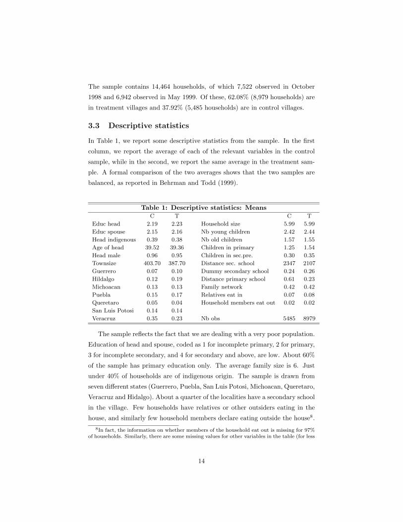
In Table 1, we report some descriptive statistics from the sample. In the first

column, we report the average of each of the relevant variables in the control

sample, while in the second, we report the same average in the treatment sam-

ple. A formal comparison of the two averages shows that the two samples are

balanced, as reported in Behrman and Todd (1999).

Table 1: Descriptive statistics: MeansC T C T

Educ head 2.19 2.23 Household size 5.99 5.99

Educ spouse 2.15 2.16 Nb young children 2.42 2.44

Head indigenous 0.39 0.38 Nb old children 1.57 1.55

Age of head 39.52 39.36 Children in primary 1.25 1.54

Head male 0.96 0.95 Children in sec.pre. 0.30 0.35

Townsize 403.70 387.70 Distance sec. school 2347 2107

Guerrero 0.07 0.10 Dummy secondary school 0.24 0.26

Hildalgo 0.12 0.19 Distance primary school 0.61 0.23

Michoacan 0.13 0.13 Family network 0.42 0.42

Puebla 0.15 0.17 Relatives eat in 0.07 0.08

Queretaro 0.05 0.04 Household members eat out 0.02 0.02

San Luis Potosi 0.14 0.14

Veracruz 0.35 0.23 Nb obs 5485 8979

The sample reflects the fact that we are dealing with a very poor population.

Education of head and spouse, coded as 1 for incomplete primary, 2 for primary,

3 for incomplete secondary, and 4 for secondary and above, are low. About 60%

of the sample has primary education only. The average family size is 6. Just

under 40% of households are of indigenous origin. The sample is drawn from

seven different states (Guerrero, Puebla, San Luis Potosi, Michoacan, Queretaro,

Veracruz and Hidalgo). About a quarter of the localities have a secondary school

in the village. Few households have relatives or other outsiders eating in the

house, and similarly few household members declare eating outside the house8.

8In fact, the information on whether members of the household eat out is missing for 97%of households. Similarly, there are some missing values for other variables in the table (for less

14

We will control for this in the empirical analysis to correct for the direct effect

on food expenditure of either. We will discuss the construction of the family

network variable below, in section 4. For now, suffices to say that there does

not appear to be a difference between the mean values of this variable in control

and treatment villlages.

3.4 Definition of Commodities and Prices

In what follows, we implement a test of collective rationality on z-conditional

demands. To do this, however, we have to consider at least two distribution

factors (which we discuss below) and two commodities. We study the demand

for the components of total food expenditure, which, in our sample, represents

about 80% of non durable expenditure on average. The PROGRESA data

contains very detailed information on food: the survey collects information on

many narrowly defined commodities and includes information both on expen-

diture and consumption. In computing the shares of the different foods, we

include a valuation of in kind consumption.

Obviously it would not be feasible to model the demand for several dozens

food items: we therefore aggregate our data to create consumption and budget

shares of 5 different commodities: (i) starches; (ii) pulses; (iii) fruit and vegeta-

bles; (iv) meat, fish and dairy; and (v) other foods. For each of the individual

commodities that make our five commodities, we compute consumption so as

to include both what has been bought and quantities obtained from own pro-

duction, payments in kind and gifts. These quantities are valued in pesos using

locality level price information derived from unit values. We take particular

care to avoid duplication induced by household production.9

Unit values are very important for our analysis and are used for two pur-

poses. First, as we mentioned above, we use them to evaluate consumption in

kind. Second, we use them to compute price indexes for each of the composite

commodities. Unit values can be computed for each household that purchases

a given commodity, dividing the value of the purchase by the quantity, as they

than 1% of the sample, information is missing for the variables recordingthe age of the headof household, the size of the town, the number of children in school, and distance to school.For family network, there are as many as 15% of missing values, as we discuss below.

9If a household has consumed some tortilla that were produced in the house, we includethe value of the tortillas (valued at average prices in the town) but do not include the valueof the flour that was purchased to make the tortillas.

15

are both reported in the survey. ‘Prices’ for individual commodities at the lo-

cality level are set at the median unit value of the households that purchased

that product in a given locality. We use medians rather than means to avoid

our estimates of prices being dominated by a few outliers in the distribution of

quantities.

Locality level prices for individual commodities are then used to compute

price indexes for each of the composite commodities, averaging individual level

prices and using as weights locality level budget shares in each of the individual

commodities. Details on the computation of the unit values and their use to

compute price indexes can be found in Attanasio et al. (2009).

Spatial and temporal differences in prices of foods mean it is important

to condition demands on prices. It is worth noting that the prices of foods

decreased considerably between October 1998 and May 1999. As mentioned

above, prices do not seem to have moved differentially between treatment and

control communities. Having said that, however, it is clear that the data present

a considerable amount of price heterogeneity across communities. To estimate

demand functions, therefore, it will be necessary to take into account price

variability even if we were considering a single cross section. The necessity to

take into account variation in prices is compounded by the fact that we use two

separate waves of the survey, October 1998 and May 1999.

3.5 Effect of the PROGRESA transfers on budget struc-ture

Given the availability of the experimental setup, we can estimate the impact of

the programme on total expenditure, on the share of food and on the share of

the five commodities in food in a very simple fashion and with a minimal set of

assumptions. The strongest of these assumptions is probably that there is no

effect (maybe through anticipation) on the control localities. 10

As the programme was randomly allocated across localities and treatment

and control samples have been proved to be well balanced in terms of baseline

characteristics, the impact of the programme on any given variable can be simply

obtained by comparing averages in treatment and control localities. In this

10Notice that this is different from the absence of spillover effects on individuals not receivingthe transfer. As the program was randomized across communities, we can allow for spillovereffects of the kind documented in these data by Angelucci and DiGiorgi (2009).

16

section, we document the effects of the programme on total consumption, the

consumption of food and the share of food. We use some of these impacts as

inputs in subsequent tests of the theoretical structure. Given a demand system

in which, say, the demand for food depends on total consumption, one could

take the impact of the programme on total consumption, feed it in an estimated

relationship and test whether the model is able to predict the change in food

consumption.

Table 2 shows averages for total non durable consumption, total food con-

sumption and the budget share of food in treatment and control villages, in Oc-

tober 1998 and in May 1999. Not surprisingly, the consumption of non durable

is considerably higher on average in treatment villages than in control villages.

In May 1999, the average difference between non durable consumption in control

and treatment villages is 16%, which, when converted in pesos, is still less than

the amount of the grant, which accounted for about 20-25% of total consump-

tion on average. This difference is estimated with considerable precision (the

standard error is 0.03) and is therefore significantly different from zero. The

increase in consumption in treatment villages in October 1998, when the pro-

gramme had only just started, is considerably smaller, but still sizeable at 8%

and statistically different from zero. Such a modest impact might be explained

by the fact that the programme was not necessarily perceived as permanent

at its inception and by administrative delays in the first few payments. The

evidence on total consumption is consistent with what has been reported in

the literature. The fact that the increase in total consumption is below the

amount of the grant has been noted and interpreted by Gertler, Martinez and

Rubio-Codina (2012), who present some interesting evidence that the part not

consumed is saved and invested in productive assets (such as small animals)

which allow a permanent increase in consumption in the long run.

The log of expenditure on food is 7% higher in treatment villages than in

control villages in 1998. The difference between treatment and control villages

increases to 16% in 1999. These average impacts of the programme, again

strongly significant, are remarkably similar to the increases in total non-durable

consumption, implying that the share of food does not change much. Indeed,

we cannot reject the hypothesis that food shares are the same in treatment and

control villages both in 1998 and 1999.

17

It is therefore the case that in Mexico, as in other countries where similar

programmes have been operating, the share of food does not decrease after

the transfer and after an increase in total consumption. This is a somewhat

surprising result: if food is a necessity, one would expect its share to decrease

with total expenditure.

Table 2: Comparison of total (log) consumption and food share

Control and treated villages in October 1998 and May 1999

October 1998 May 1999

Cont. Treat. Diff. Cont. Treat. Diff.

ln(cons. exp.) 6.71 6.80 0.08 6.69 6.85 0.16(0.47) (0.46) (0.03) (0.48) (0.49) (0.03)

ln(food exp.) 6.52 6.59 0.07 6.45 6.61 0.16(0.46) (0.46) (0.02) (0.47) (0.48) (0.02)

Share of Food 83.40 82.94 −0.45 80.04 79.48 −0.56(10.98) (11.37) (0.59) (12.19) (12.25) (0.68)

Nb of obs 2874 4798 2611 4486Budget shares are multiplied by 100; Nb in parenthesis are standard errors

for differences; standard deviations elsewhere.

Bootstrap clustered by village. 500 replications.

In Attanasio and Lechene (2010), we rule out a number of explanations

for the lack of a significant decline in the share of food as total consumption

increases, and argue that it might be explained by the fact that targeting the

cash transfer to women might have changed the balance of power within the

household. Here, we want to check whether the restrictions implied by a specific

non-unitary model of intrahousehold resource allocation, the collective model,

hold in the same data and can explain this evidence.

As discussed in Section 2, to perform this test, we need at least two dis-

tribution factors and at least two independent demand functions. The latter

and adding up of expenditure shares imply considering three commodities. One

possibility, therefore, would be to consider the demand for food and the demand

for two other commodities. However, given that food accounts for such a large

fraction of these families’ budget and the fact that the quality of the informa-

tion on non food items is not as high as that on food consumption, makes this

strategy difficult to implement in practice. Therefore, in what follows we focus

on the demand for food components. This choice is also motivated by the fact

that the information we have on unit values seems to indicate a large level of

heterogeneity in prices across villages. To test the predictions of the collective

18

model on a demand system, it will therefore be important to control for prices

and we do not have that information for non-food components of consump-

tion. Finally, as we document below, even when food consumption increases,

the programme seems to induce relatively small changes in the composition of

food consumption. It is therefore particularly interesting to check whether the

demand system we estimate is able to generate this type of patterns.

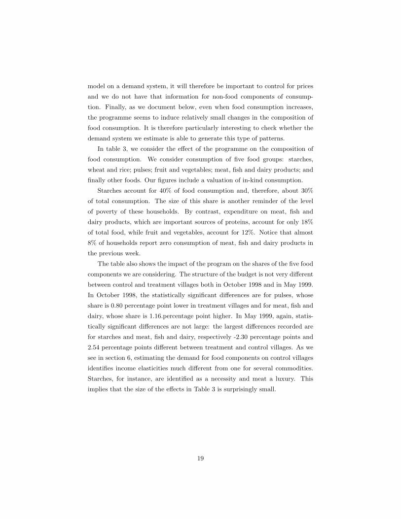
In table 3, we consider the effect of the programme on the composition of

food consumption. We consider consumption of five food groups: starches,

wheat and rice; pulses; fruit and vegetables; meat, fish and dairy products; and

finally other foods. Our figures include a valuation of in-kind consumption.

Starches account for 40% of food consumption and, therefore, about 30%

of total consumption. The size of this share is another reminder of the level

of poverty of these households. By contrast, expenditure on meat, fish and

dairy products, which are important sources of proteins, account for only 18%

of total food, while fruit and vegetables, account for 12%. Notice that almost

8% of households report zero consumption of meat, fish and dairy products in

the previous week.

The table also shows the impact of the program on the shares of the five food

components we are considering. The structure of the budget is not very different

between control and treatment villages both in October 1998 and in May 1999.

In October 1998, the statistically significant differences are for pulses, whose

share is 0.80 percentage point lower in treatment villages and for meat, fish and

dairy, whose share is 1.16.percentage point higher. In May 1999, again, statis-

tically significant differences are not large: the largest differences recorded are

for starches and meat, fish and dairy, respectively -2.30 percentage points and

2.54 percentage points different between treatment and control villages. As we

see in section 6, estimating the demand for food components on control villages

identifies income elasticities much different from one for several commodities.

Starches, for instance, are identified as a necessity and meat a luxury. This

implies that the size of the effects in Table 3 is surprisingly small.

19

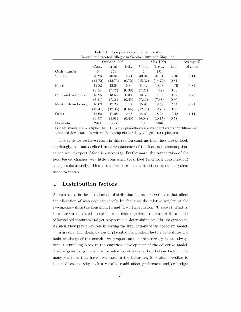
Table 3: Composition of the food basket

Control and treated villages in October 1998 and May 1999

October 1998 May 1999 Average %

Cont. Treat. Diff. Cont. Treat. Diff. of zeros

Cash transfer 0 268 0 291

Starches 40.26 40.04 -0.21 43.34 41.04 -2.30 0.14

(14.72) (13.73) (0.72) (15.37) (14.79) (0.81)

Pulses 12.82 12.03 -0.80 11.42 10.63 -0.79 3.89

(8.24) (7.72) (0.39) (7.26) (7.47) (0.35)

Fruit and vegetables 13.26 13.65 0.38 10.55 11.53 0.97 2.72

(8.61) (7.86) (0.43) (7.41) (7.38) (0.30)

Meat, fish and dairy 16.03 17.20 1.16 15.99 18.53 2.54 8.23

(12.47) (12.36) (0.64) (12.75) (12.78) (0.65)

Other 17.62 17.08 -0.53 18.69 18.27 -0.42 1.14

(9.93) (8.98) (0.49) (9.94) (10.17) (0.58)

Nb of obs 2874 4798 2611 4486

Budget shares are multiplied by 100; Nb in parenthesis are standard errors for differences;

standard deviations elsewhere. Bootstrap clustered by village. 500 replications

The evidence we have shown in this section confirms that the share of food,

suprisingly, has not declined in correspondence of the increased consumption,

as one would expect if food is a necessity. Furthermore, the composition of the

food basket changes very little even when total food (and total consumption)

change substantially. This is the evidence that a structural demand system

needs to match.

4 Distribution factors

As mentioned in the introduction, distribution factors are variables that affect

the allocation of resources exclusively by changing the relative weights of the

two agents within the household (µ and (1−µ) in equation (3) above). That is,

these are variables that do not enter individual preferences or affect the amount

of household resources and yet play a role in determining equilibrium outcomes.

As such, they play a key role in testing the implications of the collective model.

Arguably, the identification of plausible distribution factors constitutes the

main challenge of the exercise we propose and, more generally, it has always

been a stumbling block in the empirical development of the collective model.

Theory gives no guidance as to what constitutes a distribution factor. For

many variables that have been used in the literature, it is often possible to

think of reasons why such a variable could affect preferences and/or budget

20

constraints. One of the best examples, in the case of couples, is the share of

income earned by the wife. While it is plausible, and documented (Bourguignon

et al., 1993; Browning et al, 1994) that such a variable affects the distribution

of resources within the family, if preferences are non separable between female

leisure and consumption, one might find that the share of women’s income,

which is obviously related to female leisure, appears in the demand system even

if the unitary model holds.

In this section, we discuss the variables we assume to be distribution factors,

and the extent to which such an assumption is plausible. In section (6.2.2), we

document how our chosen distribution factors affect demand patterns.

The context of PROGRESA and its evaluation data set is unique in several

respects, which makes it possible to construct two convincing candidates for

distribution factors. First, women are randomly selected to participate in the

programme and to receive a cash transfer. For recipients, this leads to an

exogenous increase in the share of the household income controlled by women.

Second, the survey associated with the programme is a census of villages and

it is possible to establish family ties of individuals in the villages. We use

this information to construct a measure of family networks for both spouses,

which we argue influence individual weights in the intra-household allocation

of resources. The distribution factors we use in what follows are receipt of the

PROGRESA transfer and the relative importance of the husband and wife’s

networks of relatives, in terms of size or of financial prowess.

4.1 Receipt of PROGRESA transfer

Eligibility for PROGRESA within a village targeted by the programme was

based on a multi-dimensional assessment of household’s poverty. Women in

eligible households were entitled to receive a cash transfer. However, within

villages included in the evaluation survey, based on eligibility for the programme,

effective receipt of the cash transfer was randomised across villages.

The motivation for targeting women as recipient of a transfer based on an

assessment of the household’s poverty, was an explicit attempt, on the part of

the administration of the programme, to improve the condition of women within

the household in rural Mexico. Therefore, unless a woman was controlling 100%

of the household income independently from PROGRESA, receipt of the PRO-

21

GRESA transfer corresponds to an increase in the share of household income

she controls. Furthermore, because of the randomisation of the programme,

PROGRESA generates an exogenous increase in the share of income controlled

by the wife only for women in some of the surveyed villages.

The share of income controlled by the wife is not an argument of preferences,

and conditional on total income, it does not affect the budget constraint. Thanks

to the exogenous variation in this variable induced by the randomisation of the

programme, PROGRESA assignment constitutes an ideal distribution factor.

Of course, the PROGRESA grant affects the total amount of resources that

a household receives and, therefore, affects the budget constraint. However,

if the demand system one uses is correctly specified, controlling for total ex-

penditure should take care of this increase in resources. Conditional on total

expenditure, whether a household receives or not PROGRESA grants should

make no difference to the allocation of total expenditures among different com-

modities. In other words, if the standard model is correctly specified, one should

be able to describe how shares change upon receiving PROGRESA grants by

movements along the Engel curve and predict them conditioning on the effect

that the program has on total expenditure.

If, instead, after conditioning on total expenditure (including that induced

by the programme) in a flexible and yet theory consistent fashion, PROGRESA

has an impact on commodity shares, it has to be because it shifts the Engel

curves, possibly as a consequence of a shift of Pareto weigths within the house-

holds. Therefore, assignment to PROGRESA is a distribution factor as, within

a unitary model, it should not affect share equations once the effect on total

expenditure is taken into account.

There are two additional caveats that need to be made to this argument. As

discussed above, the PROGRESA grant is a conditional cash transfer, where

some conditions, namely the enrollment in school of the household children,

might be related to certain expenditures. However, the argument we have

sketched above holds conditional on school enrolment behaviour. For this rea-

son, in what follows, we estimate a conditional demand system where we con-

sider expenditure shares conditional on schooling behaviour. Analogously, if the

receipt of the PROGRESA transfer affected labour supply, then it would not

be a valid distribution factor. The experimental evidence on PROGRESA has

22

not shown any impacts on adult labour supply (see Skoufias, 2001 and Skoufias

and Di Maro, 2008).

4.2 Relative importance of family networks.

The second distribution factor we consider is the relative importance of hus-

band’s and wife’s networks. The main idea behind the use of the relative im-

portance of the networks is the fact that the presence of such networks may

impact, for a variety of possible reasons, on the balance of power within the

household. It is plausible to assume that the position within the household and

the relative weights of husband and wife in the allocation of resources depend,

within the context of the rural villages we are studying, on the relative strength

and influence of the two extended families in the village. A woman who can

count on a network of siblings and relatives larger, wealthier and more resource-

ful than that of her husband is likely to be in a stronger position in the allocation

of resources within the household. On the other hand, having a relatively larger

and impoverished extended family network can arguably weaken one’s position

within the household.

Before justifying fully the use of such a variable as a distribution factor, we

first describe how we construct it and present some descriptive statistics on it.

To construct the relative importance of the spouses’s networks we use an idea

developed in an innovative paper by Angelucci, De Giorgi, Rangel and Rasul

(2009) (ADRR09, from now on). ADDR09 use the fact that the PROGRESA

evaluation survey is a census within each locality and the convention of Spanish

last names to map the network of siblings and cousins within each community.

In Spanish speaking countries, individuals get two surnames. The first is the

(first) surname of their father, while the second is the (first) surname of their

mother. As in one of the waves of PROGRESA, both surnames of all individuals

are available, one can identify the family network for a large fraction of the

sample households. We construct an algorithm which is very similar to that

used by ADDR08 and construct, for each individual in the evaluation sample,

the number of siblings and cousins that are present in the same locality.

We use these data to construct our candidate distribution factor, the relative

importance of husband and wife’s networks, in two ways: the size and the wealth

of the networks. The former is the relative number of siblings residing in the

23

same village, s2/(s1 + s2), where si, i = 1, 2 is the number of siblings of the

wife and the husband respectively. We can also take into account the relative

economic resource of the siblings and not only their number. More specifically,

we construct a second index as the ratio of the (food) consumption of the wife’s

siblings over the (food) consumption of all siblings (husband and wife), where

consumption is proxying for wealth.

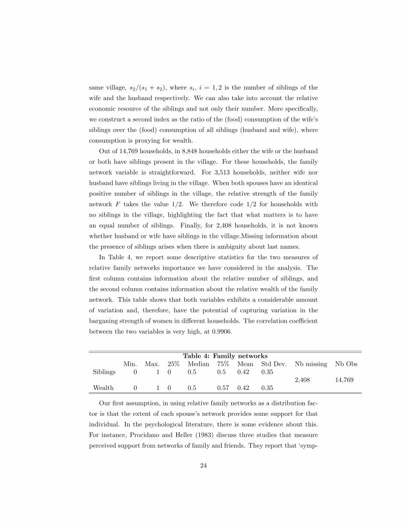
Out of 14,769 households, in 8,848 households either the wife or the husband

or both have siblings present in the village. For these households, the family

network variable is straightforward. For 3,513 households, neither wife nor

husband have siblings living in the village. When both spouses have an identical

positive number of siblings in the village, the relative strength of the family

network F takes the value 1/2. We therefore code 1/2 for households with

no siblings in the village, highlighting the fact that what matters is to have

an equal number of siblings. Finally, for 2,408 households, it is not known

whether husband or wife have siblings in the village.Missing information about

the presence of siblings arises when there is ambiguity about last names.

In Table 4, we report some descriptive statistics for the two measures of

relative family networks importance we have considered in the analysis. The

first column contains information about the relative number of siblings, and

the second column contains information about the relative wealth of the family

network. This table shows that both variables exhibits a considerable amount

of variation and, therefore, have the potential of capturing variation in the

barganing strength of women in different households. The correlation coefficient

between the two variables is very high, at 0.9906.

Table 4: Family networksMin. Max. 25% Median 75% Mean Std Dev. Nb missing Nb Obs

Siblings 0 1 0 0.5 0.5 0.42 0.352,408 14,769

Wealth 0 1 0 0.5 0.57 0.42 0.35

Our first assumption, in using relative family networks as a distribution fac-

tor is that the extent of each spouse’s network provides some support for that

individual. In the psychological literature, there is some evidence about this.

For instance, Procidano and Heller (1983) discuss three studies that measure

perceived support from networks of family and friends. They report that ‘symp-

24

toms of distress and psychopatology’ were inversely related to both measures

of network support but the relationship was particularly strong for family net-

works. We argue, therefore, that the relative size of the network will affect the

relative position of the spouses in the household.11

As an additional check on whether the relative size of the spouses network

affects the relative position of the spouses in the household, we use some infor-

mation on decision making that is elicited in the evaluation survey. In particu-

lar, there are several questions about who makes decisions about certain issues

(such as making major purchases, taking the children to the doctor, allocating

additional resources), where the possible answers are ’the wife’, the ’husband’

or both. We construct an index of the bargaining power of the woman and

regress it on the relative network size to find that the two variables seem to

be associated. Incidentally, the same index is also affected by the assignment

to PROGRESA. This evidence (available upon request) supports our choice of

distribution factors.

For the relative importance of the family network to be a valid distribution

factor, it has to be excluded from preferences and from the budget constraint,

and yet influence choices. We document in section 6.2.2 the extent to which the

relative importance of the family network influences choices. Here, we discuss

why it can be excluded from both the budget constraint and preferences.

The number of siblings (of either or both spouses) might have a direct effect

on the demand for food, if siblings share meals. Whilst this would not invalidate

the relative size of the family network as a distribution factor, not accounting

for the direct effect of the number of siblings on the demand for food might

would bias the estimates.To avoid this potential bias, we control for the number

of relatives who share meals with the household as a determinant of expenditure

shares. The survey contains explicit information on this variable.

There might furthermore be reasons for the size of the spouses networks to

affect the demand system outside of the collective framework. Three reasons

come to mind: altruism, the reciprocity of caring and risk sharing possibilities.

In the presence of altruism, one could argue that a relatively large number of

11Several papers in the literature have looked at the effects that family networks have onvarious aspects of household behaviour, such as consumption and risk sharing (Altonji etal., 1992); inter-generational transfers (Altonji et al., 1997; Behrman and Rosenzweig 2006;Cox and Jakubson, 1995; La Ferrara, 2003); children’s education choices (Loury, 2006); andnon-resident parental investments into children (Weiss and Willis, 1985).

25

relatives of, say, the wife, would give more weight to wife’s preferences even if

the right model is a unitary one. Moreover, if women care about their siblings,

presumably their siblings care for them. Then, the number of siblings might

affect preferences rather than bargaining, if women’s preferences are different

depending upon the number of siblings they have. Similarly, if there is insurance

between households, the size of family networks might be related to the necessity

of sharing risk.12

We ignore these worries for several reasons. First, these arguments refer to

the size of the network rather than to the relative size of husband’s and wife’s

networks. Second, if altruism effects are additive these considerations will not

affect the demand system. Third, and especially relevant for risk sharing, we are

considering the effect of distribution factors on expenditure shares, conditional

on the level of total expenditure. The latter is more likely to be affected by the

size of networks, maybe because of risk sharing considerations. For expendi-

ture shares, however, standard two stage budgeting considerations make it less

obvious that the relative size of networks would have a direct effect, once one

conditions on total consumption.

5 The Demand System: Methodological issues

We model the demand for the components of food consumption, ignoring non-

food consumption, partly because we do not observe the prices of non food

consumption and partly because the quality of the non-food data is not as high

as that for food items. We assume two stage budgetting and separability of food

from the rest of consumption and labour supply, so that the shares of the various

components of food consumption are functions of total food consumption, de-

mographics, relative prices and, possibly, distribution factors. Given that food

constitutes a very large fraction of total consumption for these households, this

is a meaningful exercise in this context.

The estimation of a demand system on data such as PROGRESA raises

methodological issues, most of which have been addressed in previous papers,

among which Attanasio and Lechene (2002 and 2010) and Attanasio, Di Maro,

Lechene and Phillips (2009, 2013). Specific additional issues arise in the im-

12Rosenzweig and Stark (1989) presente evidence that, in South India, women might tendto marry to far away villages by the need to insure large idiosycnratic risks.

26

plementation of a test of collective rationality. We review these methodological

issues here, starting with the functional form of the demand system, followed

by the endogeneity of total expenditure, of the conditioning good and of school-

ing. Finally, we discuss separability in the collective model, and the question of

endogeneity of prices.

5.1 Functional form of the demand system

We estimate a Quadratic Almost Ideal Demand System (QUAIDS, Banks, Blun-

dell and Lewbell (1997)) which allows for quadratic effects in total expendi-

ture. Allowing for quadratic effects is particularly important in our context

where we want to predict changes in expenditure shares related to a relatively

large change in total (food) consumption. In Attanasio, Di Maro, Lechene and

Phillips (2009), we find that it is important to allow for income responses to

vary with the level of income as permitted by a QUAIDS when estimating a

demand system on the PROGRESA data.

The QUAIDS can be derived from the maximization of a unitary utility

function, in which case, the coefficients on the vector of prices have to satisfy

a number of restrictions (so that, for instance, the resulting Slutsky matrix is

symmetric and negative definite). In the context of a collective model with

public goods within the family, the shape of the demand functions that would

arise is not obvious, even when both agents have preferences that would give

rise to a QUAIDS in the unitary case.

In our application, following Browning and Chiappori (1998) and Attanasio,

Di Maro, Lechene and Phillips (2009), we specify a QUAIDS, in which expen-

diture shares are allowed to depend on log total (food) consumption and its

square, on prices and on demographics, as they would in a standard QUAIDS.

We do not impose symmetry of the Slutsky matrix, but only homogeneity and

adding-up. 13 We also allow the effect of the two distribution factors we consider

and assume that they enter the demand system additively.

13Browning and Chiappori (1998) show that symmetry does not hold in the collective model,but that the Pseudo-Slutsky matrix of price responses is the sum of a symmetric matrix anda rank one matrix and, in their empirical application, have used the QUAIDS specification asa useful parametrization of the household demand function.Browning and Chiappori (1998)’srestrictions on the Slutsky matrix from the demand system of a collective model can also betested. We leave that exercise, however, for future work.

27

In particular, we estimate the following approximation to a QUAIDS

wi = θ′iz + φ′id+

n∑j=1

γij ln(pj) + βi ln

(x

a(p)

)+ λi

(ln

(x

a(p)

))2

+ ui (8)

where wi is the share of commodity i in total expenditure on goods, i = 1, ...n,

x is total expenditure on goods and the price index a(p) is approximated by a

Stone price index where expenditure shares are used as weights. d is a vector of

demographic variables and z a vector of distribution factors, θi and φi are vectors

of parameters. The variable ui represents unobserved taste heterogeneity.

The ’intercept’ in equation (8) is a function of the distribution factors z and

of various demographic variables that represent shocks to tastes . The latter

include the number of young children, controls for the education of the head of

household and his spouse, for the age of the head of household, for whether the

head of household is indigenous and the size of the town. We also control for

household members eating out and for relatives eating in.

What distinguishes distribution factors z from demographics d is the fact

that there are additional restrictions in the manner in which they enter into

the demand functions. These restrictions are equivalently the proportionality

restrictions or the restrictions on conditional demands, as we saw in section 2.3.

The assumption of an additive effect of distribution factors on a (QU)AIDS is

somewhat arbitrary. Nothing prevents the distribution factors to affect demands

in more complicated manners. For instance, it could be that they enter demands

multiplicatively on total expenditure. In that case the restrictions to be tested

are much more complicated. However, we did not find significant interaction

effects between distribution factors and expenditure. In other words, the distri-

bution factors affect the intercept but not the slope of the Engel curves. We did

not investigate the possibility that distribution factors affect price elasticities.

Under the unitary model, the two distribution factors we consider should not

enter the demand system, so that the evidence we present also constitutes a test

of the unitary model. The collective model imposes cross-equation restrictions

on θi that we will test in section 6.3.

5.2 Endogeneity of total expenditure

We model the five components of food as a function of total food consumption,

under the assumption of two stage budgeting. Households first decide how much

28

to allocate to food and then, conditional on total food expenditure, how much

to allocate to each food component. The residuals of our equations can be

interpreted as unobservable components of tastes that affect budget shares. If

taste shocks to the system that determines total food consumption are correlated

to the unobserved shocks to food components, then total food will be endogenous

in our system. Measurement error in total expenditure is also a likely cause of

endogeneity.

An instrument for total expenditure often used in the literature is house-

hold income, which implicitely assumes that the measurement error in total

expenditure is uncorrelated with measured income. Under the assumption that

heterogeneity in tastes is the source of endogeneity of total expenditure, income

is a valid instrument if labour supply is separable from consumption. It may be

worthwhile to make explicit and formal these arguments. Suppose the household

maximizes expected utility subject to an intertemporal budget constraint:

MaxE0

T∑t=1

β(zt, vt)U(qt, et, lt, ut,dt, zt). s.t.

ptqt = xt

xt + St = wt(T − lt) + yt + (1 + r)St−1

where U() is a household utility function which might be collective or unitary;

q and p are vectors of commodities and prices, x total expenditure, w wages, h

hours worked, y non labour income, S savings, d some demographic variables,

z distribution factors in the case of a collective model, v is an intertemporal

taste shock and e and u are taste shocks that affect the marginal utility of

commodities and labour respectively. By two-stage budgeting, one could think

that first the household members choose total expenditure and then how to

allocate it among different commodities. If the function U can be written as:

U(qt, et, ht, ut) = u(qt, et,dt, zt) + V (ht, ut,dt, zt)

one can decouple the labour supply problem from the determination of total

expenditure and the allocation of the latter across different commodities. Total

expenditure would still be endogenous if the vector of unobservable taste shocks

e is correlated in the cross section with the intertemporal taste shock v. In such

a situation, total household income wt(T− lt)+yt can be used as an instrument,

if one assumes that the taste shock ut is uncorrelated with the vector et.

29

If one thinks that such an assumption is too strong, a possible alternative is

to use the component of income that the household takes as given (the wages)

as an instrument for total expenditure. We considered the average agricultural

wage in a village as an instrument. Such a variable would be a valid instrument

(under separability) even when the three taste shocks we consider (u, e and v)

are correlated.

There is an additional reason to consider aggregate wages (rather than indi-

vidual income) as an instrument for total expenditure. Income can be a weak

instrument in a context where large transitory shocks or measurement error

may weaken the relationship between income and total expenditure. This ar-

gument is particularly relevant in the context of developing countries where,

while consumption is relatively simple to measure, income (and its many com-

ponents) might be difficult to capture. In Attanasio and Lechene (2002), we

find that individual level expenditure is better explained by average wages than

by individual income in the cross section.

Obviously, by using average wages, we loose the variability at the individual

level since, in this case, we only exploit the variation across villages. However,

given the high variance of measurement error in income, this is not necessarily a

problem. We find that once we introduce distribution factors in the model, only

results obtained with the village average agricultural wage are robust across

different dimensions.

If consumption and leisure are not separable in the utility function, income or

wages are not valid instruments for total expenditure. However, in that case, the

entire demand system is mispecified as one should allow for the effect of hours

of work on the marginal utility of consumption. Hours of work should enter in

their own right as a determinant of the demand system. In the context we are

studying we have decided to assume separability of food consumption from non

food consumption and leisure for two reasons. First, labour supply behaviour is

likely to be fairly inelastic in the present context for the poor households in our

sample. Considering it as separable from consumption, therefore, might not be

a bad approximation. Second, as we focus on the role of Oportunidades as a

distribution factor in the demand system, we can appeal to the fact (reported

in the literature, see Skoufias (2001) and Skoufias and DiMaro (2008)) that the

programme has not affected adult labour supply.

30

5.3 Endogeneity of conditioning good in z-conditional test

An additional endogeneity issue arises when we estimate the z-conditional de-

mand system in equation 7, as the conditioning good j is correlated with the

unobserved taste shock of the demand for good i. The instrument that identifies

the model is suggested directly by the theory and by the test we propose: if the

collective model is valid, the distribution factor used for inverting the demand

of the conditioning good is a valid instrument as, conditional on the demand for

commodity j in equation 7, no distribution factor affects the demand for any

commodity i 6= j. This is the sense of the test in equation 6. The distribution

factor used to invert the demand for commodity j is therefore a valid instru-

ment for Cj in equation 7. We can use the significance of the second distribution

factor (in our case the PROGRESA/Oportunidades indicator) as a test of the

validity of the model.

5.4 Schooling

Conditional cash transfer programmes impose minimum schooling requirements

for children of the recipient households to receive the largest component of the

grant. The grant amounts are devised with the aim to cover the opportunity

cost of schooling for the household, which is why they vary with the age and

gender of the child. The conditionality might affect consumption behaviour, if

sending children to school imposes related costs, such as for uniforms, shoes or

books. Conversely, children might be fed in school, which would also have an

impact on the budget share of food and its components. It is thus necessary

to control for schooling of children, over and above controlling for household

composition. However, it could be that unobserved taste for school is correlated

with unobserved taste for certain foods, so that schooling could be endogenous in

the demand system. To allow for this possibility, we instrument schooling with

an indicator for the existence of a secondary school and distance from secondary

school if it is not in the village (and zero if it is in the village). The average

distance to a secondary school is 2.2 kilometers, with a maximum distance of

14 kilometers. In only about 25% of villages is there a secondary school.

The assumption that we are making is that the distance to a secondary school

affects schooling decisions but does not affect the structure of expenditures

between foods, conditional on the size of the village and the other controls

31

in the demand system. As is always the case, it is not possible to test the

identification restriction that we are using. One possible worry, for instance,

is that the presence of a school in a nearby village proxies for other variables

(such as the presence of a market) that might affect demand. However, we feel

that conditional on village size and the other variables (including prices) we

are considering, the information on the distance to a secondary school can be

excluded from the demand system.

Primary school is not considered as endogenous in the demand system. Pri-

mary school attendance is high (over 90%) and not affected by the programme.

However, we follow previous literature on PROGRESA in that we condition on

the number of children attending primary school in the demand system, for the

reasons mentioned above.

5.5 Additional issues

There are two additional methodological issues worth mentioning briefly. The

first one has to do with separability in the collective model. When considering

the collective model, assuming that individual preferences are separable between

food and the rest is not sufficient to get a household demand system for food

components that does not depend on non-food relative prices. To obtain such a

specification, we need to make an additional assumption, namely that the shar-

ing rule or Pareto weights of the individuals in the household welfare function

do not depend on the prices of non-food items. This is true if the household

decides on the allocation of the total between food and non food, and then on

the allocation between foods. Following this argument, the Pareto weight, or

the sharing rule for this problem will depend on the prices of the foods, and the

total expenditure on the same, and the distribution factors if any.

The second methodological issue is the possible endogeneity of prices. Sup-

pose that tastes shocks are correlated within villages. In this case, it could be

that in a village where people like meat a lot, the price of meat will be high

and yet, there will be a high demand for meat. One way around this would

be to instrument prices with supply conditions (number of shops, distance from

big markets, etc...). We do not have this information, and we therefore make

the assumption that this effect is absent. We should also note that our main

interest is in the effect that the introduction of PROGRESA has on the demand

32

system and that studies that have looked at the effect of PROGRESA on prices

(such as Angelucci and DeGiorgi, 2009) have not found any effects.

6 Empirical results

We divide this section in three parts. First, we present results for the first stage

regressions we estimate to deal with the endogeneity of total food consumption

and school enrolment. We then discuss our estimates of the demand systems

and informally compare the predictions implied by the model for the impact of

the grant on consumption shares. Finally, we present the formal tests of the

restrictions of the collective model.

6.1 First stage regressions

As we discussed in the previous section, there are two potentially endogenous

variables in the demand system: total expenditure on food and number of chil-

dren in secondary and ”preparatoria” school. Table 5 shows the first stage

regressions for the log of total expenditure and the number of children in sec-

ondary school and ”preparatoria” school. These regressions include both the

instruments and the other conditioning variables that enter the second stage.

In the first two columns of the table, the instrument for total expenditure is the

village average agricultural wage, whilst in the last two columns, it is household

income. The other instruments we use (for secondary school enrolment) are an

indicator of the presence of a secondary school and the distance to the secondary

school.

The results reported in Table 5 refer to the entire sample, which includes

both treatment and control localities. Results on the control sample, for which

we report estimates of the demand system in the next section, are substantially

similar and are available upon request.

The instruments have the expected effects in the first stage regressions. In

the equation for log total expenditure, we find that both village median agri-

cultural wage and income have power in explaining total food expenditure and

that both the linear and the quadratic terms are important. As for the equa-

tion for secondary school enrolment, we find that distance to secondary school

influences the number of children attending secondary school in the expected

direction.

33

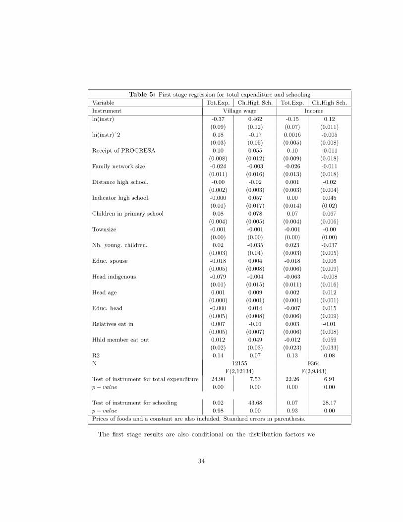
Table 5: First stage regression for total expenditure and schooling

Variable Tot.Exp. Ch.High Sch. Tot.Exp. Ch.High Sch.

Instrument Village wage Income

ln(instr) -0.37 0.462 -0.15 0.12

(0.09) (0.12) (0.07) (0.011)

ln(instr)ˆ2 0.18 -0.17 0.0016 -0.005

(0.03) (0.05) (0.005) (0.008)

Receipt of PROGRESA 0.10 0.055 0.10 -0.011

(0.008) (0.012) (0.009) (0.018)

Family network size -0.024 -0.003 -0.026 -0.011

(0.011) (0.016) (0.013) (0.018)

Distance high school. -0.00 -0.02 0.001 -0.02

(0.002) (0.003) (0.003) (0.004)

Indicator high school. -0.000 0.057 0.00 0.045

(0.01) (0.017) (0.014) (0.02)

Children in primary school 0.08 0.078 0.07 0.067

(0.004) (0.005) (0.004) (0.006)

Townsize -0.001 -0.001 -0.001 -0.00

(0.00) (0.00) (0.00) (0.00)

Nb. young. children. 0.02 -0.035 0.023 -0.037

(0.003) (0.04) (0.003) (0.005)

Educ. spouse -0.018 0.004 -0.018 0.006

(0.005) (0.008) (0.006) (0.009)

Head indigenous -0.079 -0.004 -0.063 -0.008

(0.01) (0.015) (0.011) (0.016)

Head age 0.001 0.009 0.002 0.012

(0.000) (0.001) (0.001) (0.001)

Educ. head -0.000 0.014 -0.007 0.015

(0.005) (0.008) (0.006) (0.009)

Relatives eat in 0.007 -0.01 0.003 -0.01

(0.005) (0.007) (0.006) (0.008)

Hhld member eat out 0.012 0.049 -0.012 0.059

(0.02) (0.03) (0.023) (0.033)

R2 0.14 0.07 0.13 0.08

N 12155 9364

F(2,12134) F(2,9343)

Test of instrument for total expenditure 24.90 7.53 22.26 6.91

p− value 0.00 0.00 0.00 0.00

Test of instrument for schooling 0.02 43.68 0.07 28.17

p− value 0.98 0.00 0.93 0.00

Prices of foods and a constant are also included. Standard errors in parenthesis.

The first stage results are also conditional on the distribution factors we

34

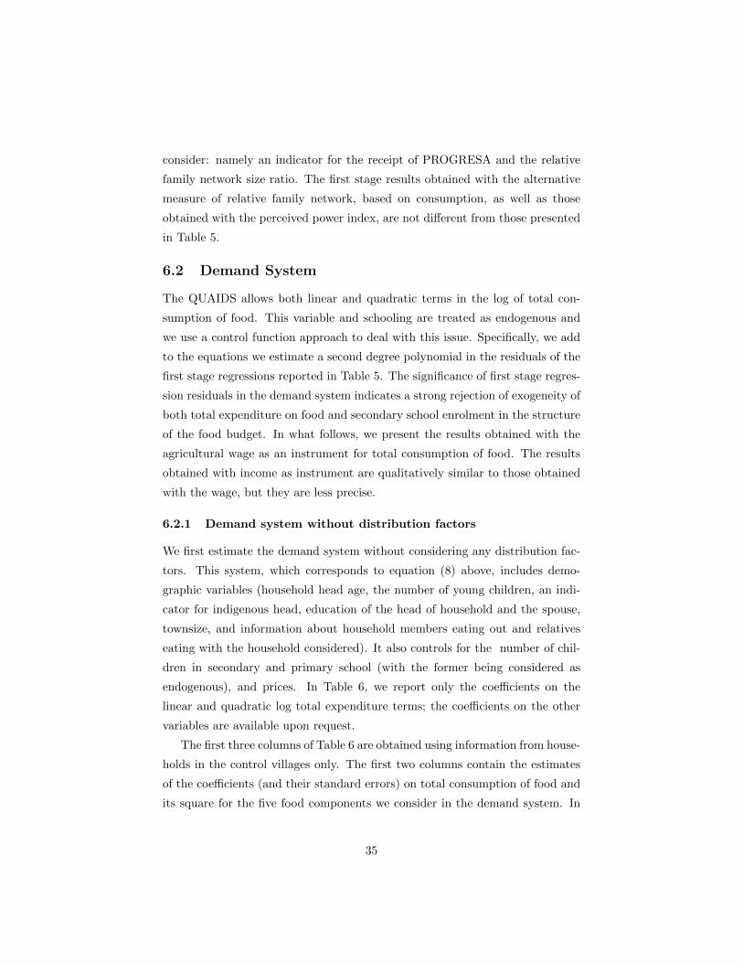
consider: namely an indicator for the receipt of PROGRESA and the relative

family network size ratio. The first stage results obtained with the alternative

measure of relative family network, based on consumption, as well as those

obtained with the perceived power index, are not different from those presented

in Table 5.

6.2 Demand System

The QUAIDS allows both linear and quadratic terms in the log of total con-

sumption of food. This variable and schooling are treated as endogenous and

we use a control function approach to deal with this issue. Specifically, we add

to the equations we estimate a second degree polynomial in the residuals of the

first stage regressions reported in Table 5. The significance of first stage regres-

sion residuals in the demand system indicates a strong rejection of exogeneity of

both total expenditure on food and secondary school enrolment in the structure

of the food budget. In what follows, we present the results obtained with the

agricultural wage as an instrument for total consumption of food. The results

obtained with income as instrument are qualitatively similar to those obtained

with the wage, but they are less precise.

6.2.1 Demand system without distribution factors

We first estimate the demand system without considering any distribution fac-

tors. This system, which corresponds to equation (8) above, includes demo-

graphic variables (household head age, the number of young children, an indi-

cator for indigenous head, education of the head of household and the spouse,

townsize, and information about household members eating out and relatives

eating with the household considered). It also controls for the number of chil-

dren in secondary and primary school (with the former being considered as

endogenous), and prices. In Table 6, we report only the coefficients on the

linear and quadratic log total expenditure terms; the coefficients on the other

variables are available upon request.

The first three columns of Table 6 are obtained using information from house-

holds in the control villages only. The first two columns contain the estimates

of the coefficients (and their standard errors) on total consumption of food and

its square for the five food components we consider in the demand system. In

35

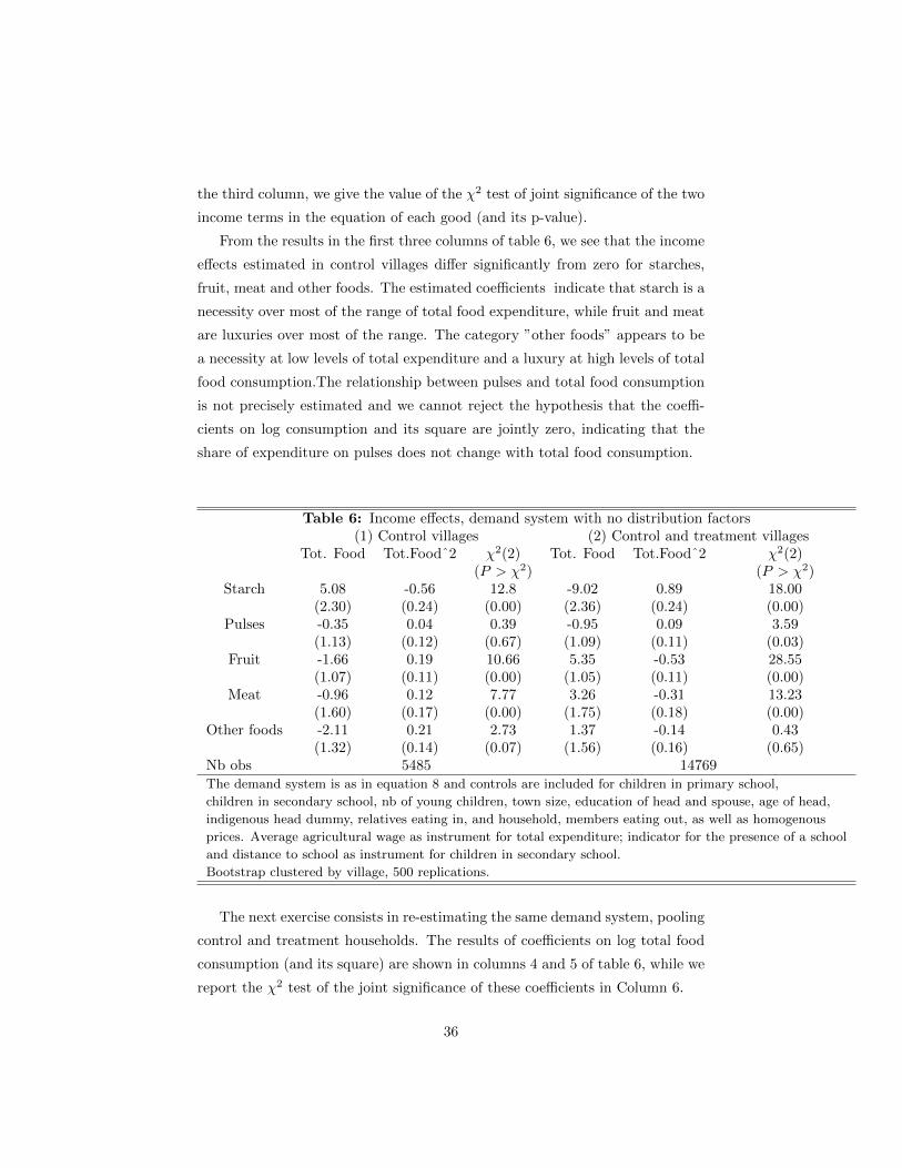
the third column, we give the value of the χ2 test of joint significance of the two

income terms in the equation of each good (and its p-value).

From the results in the first three columns of table 6, we see that the income

effects estimated in control villages differ significantly from zero for starches,

fruit, meat and other foods. The estimated coefficients indicate that starch is a

necessity over most of the range of total food expenditure, while fruit and meat

are luxuries over most of the range. The category ”other foods” appears to be

a necessity at low levels of total expenditure and a luxury at high levels of total

food consumption.The relationship between pulses and total food consumption

is not precisely estimated and we cannot reject the hypothesis that the coeffi-

cients on log consumption and its square are jointly zero, indicating that the

share of expenditure on pulses does not change with total food consumption.

Table 6: Income effects, demand system with no distribution factors(1) Control villages (2) Control and treatment villages

Tot. Food Tot.Foodˆ2 χ2(2) Tot. Food Tot.Foodˆ2 χ2(2)(P > χ2) (P > χ2)

Starch 5.08 -0.56 12.8 -9.02 0.89 18.00(2.30) (0.24) (0.00) (2.36) (0.24) (0.00)

Pulses -0.35 0.04 0.39 -0.95 0.09 3.59(1.13) (0.12) (0.67) (1.09) (0.11) (0.03)

Fruit -1.66 0.19 10.66 5.35 -0.53 28.55(1.07) (0.11) (0.00) (1.05) (0.11) (0.00)

Meat -0.96 0.12 7.77 3.26 -0.31 13.23(1.60) (0.17) (0.00) (1.75) (0.18) (0.00)

Other foods -2.11 0.21 2.73 1.37 -0.14 0.43(1.32) (0.14) (0.07) (1.56) (0.16) (0.65)

Nb obs 5485 14769The demand system is as in equation 8 and controls are included for children in primary school,

children in secondary school, nb of young children, town size, education of head and spouse, age of head,

indigenous head dummy, relatives eating in, and household, members eating out, as well as homogenous

prices. Average agricultural wage as instrument for total expenditure; indicator for the presence of a school

and distance to school as instrument for children in secondary school.

Bootstrap clustered by village, 500 replications.

The next exercise consists in re-estimating the same demand system, pooling

control and treatment households. The results of coefficients on log total food

consumption (and its square) are shown in columns 4 and 5 of table 6, while we

report the χ2 test of the joint significance of these coefficients in Column 6.

36

The treatment consists in the injection of (relatively) large amounts of cash

in the budget of treated households. As the treatment was allocated randomly,

if the structural model we estimated was well specified, including the treated

households in the estimation sample should not make much difference to the

point estimates of the income effects, but should increase their precision. What

we find, however, is different. Rather than increasing precision, increasing the

sample size by incorporating poor households from the treated villages leads

to changes in the values of the estimated coefficients. We interpret this lack

of stability as indicating that the model is not able to capture the relationship

between total expenditure and the structure of the budget following the cash

transfers.

We further substantiate our interpretation of these results, by using the

estimates from Table 6 and the estimated experimental impact on total food

consumption (and schooling) to predict the impact of the PROGRESA grant

on the shares of the five commodities that we are considering. We do this in

Tables 7 and 8, respectively for October 1998 and May 1999.

In the first column of the tables, we report the average impact of the program

as estimated comparing treatment and control communities. We will be referring

to this impact as the ‘actual’ impact, as it is based on experimental evidence. As

discussed in section (3.5), what is most notable about the actual impacts of the

cash transfers on the structure of the budget is how small they are. The budget

share of starch is 2.30 percentage point lower in treated households than it is in

control households in May 1999. This is consistent with the fact that starch has

been found to be a necessity. The share of pulse also decreases significantly at

both dates, albeit not dramatically. The shares of fruits and especially of meat

increase.

In the second column of Tables 7 and 8, we use the estimates of the demand

system estimated using only data from control villages (and reported in the first

two columns of Table 6) to predict the impacts of the program on expenditure

shares. In the third column of Tables 7 and 8, we use the estimates of the

demand system obtained from both treatment and control villages. In terms

of point estimates, the predictions are of poor quality for all the goods at both

dates. However, note that since the actual impacts are mostly zero, we are

trying to predict zero, which can arise also through lack of precision.

37

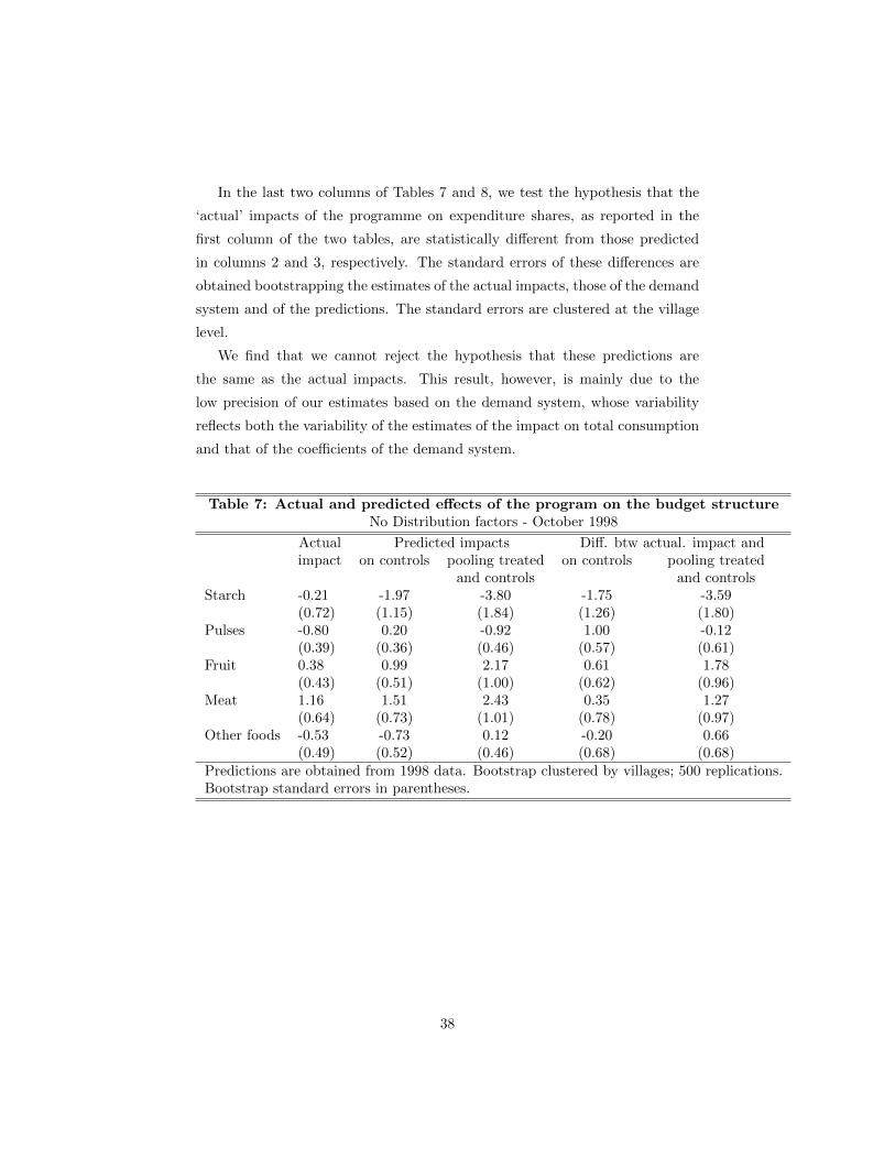
In the last two columns of Tables 7 and 8, we test the hypothesis that the

‘actual’ impacts of the programme on expenditure shares, as reported in the

first column of the two tables, are statistically different from those predicted

in columns 2 and 3, respectively. The standard errors of these differences are

obtained bootstrapping the estimates of the actual impacts, those of the demand

system and of the predictions. The standard errors are clustered at the village

level.

We find that we cannot reject the hypothesis that these predictions are

the same as the actual impacts. This result, however, is mainly due to the

low precision of our estimates based on the demand system, whose variability

reflects both the variability of the estimates of the impact on total consumption

and that of the coefficients of the demand system.

Table 7: Actual and predicted effects of the program on the budget structureNo Distribution factors - October 1998

Actual Predicted impacts Diff. btw actual. impact andimpact on controls pooling treated on controls pooling treated

and controls and controlsStarch -0.21 -1.97 -3.80 -1.75 -3.59

(0.72) (1.15) (1.84) (1.26) (1.80)Pulses -0.80 0.20 -0.92 1.00 -0.12

(0.39) (0.36) (0.46) (0.57) (0.61)Fruit 0.38 0.99 2.17 0.61 1.78

(0.43) (0.51) (1.00) (0.62) (0.96)Meat 1.16 1.51 2.43 0.35 1.27

(0.64) (0.73) (1.01) (0.78) (0.97)Other foods -0.53 -0.73 0.12 -0.20 0.66

(0.49) (0.52) (0.46) (0.68) (0.68)Predictions are obtained from 1998 data. Bootstrap clustered by villages; 500 replications.Bootstrap standard errors in parentheses.

38

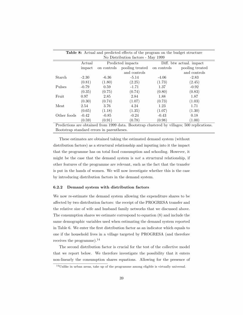
Table 8: Actual and predicted effects of the program on the budget structureNo Distribution factors - May 1999

Actual Predicted impacts Diff. btw actual. impactimpact on controls pooling treated on controls pooling treated

and controls and controlsStarch -2.30 -6.36 -5.14 -4.06 -2.83

(0.81) (1.80) (2.25) (1.73) (2.45)Pulses -0.79 0.59 -1.71 1.37 -0.92

(0.35) (0.75) (0.74) (0.80) (0.83)Fruit 0.97 2.85 2.84 1.88 1.87

(0.30) (0.74) (1.07) (0.73) (1.03)Meat 2.54 3.76 4.24 1.23 1.71

(0.65) (1.18) (1.35) (1.07) (1.30)Other foods -0.42 -0.85 -0.24 -0.43 0.18

(0.59) (0.91) (0.78) (0.98) (1.00)Predictions are obtained from 1999 data. Bootstrap clustered by villages; 500 replications.Bootstrap standard errors in parentheses.

These estimates are obtained taking the estimated demand system (without

distribution factors) as a structural relationship and inputing into it the impact

that the programme has on total food consumption and schooling. However, it

might be the case that the demand system is not a structural relationship, if

other features of the programme are relevant, such as the fact that the transfer

is put in the hands of women. We will now investigate whether this is the case

by introducing distribution factors in the demand system.

6.2.2 Demand system with distribution factors

We now re-estimate the demand system allowing the expenditure shares to be

affected by two distribution factors: the receipt of the PROGRESA transfer and

the relative size of wife and husband family networks that we discussed above.

The consumption shares we estimate correspond to equation (8) and include the

same demographic variables used when estimating the demand system reported

in Table 6. We enter the first distribution factor as an indicator which equals to

one if the household lives in a village targeted by PROGRESA (and therefore

receives the programme).14

The second distribution factor is crucial for the test of the collective model

that we report below. We therefore investigate the possibility that it enters

non-linearly the consumption shares equations. Allowing for the presence of

14Unlike in urban areas, take up of the programme among eligible is virtually universal.

39

quadratic (or higher order) terms is important for two reasons. First, the theory

is silent about the specific form in which this (or any other) distribution factors

enters the share equations. Second, the test of the collective model we propose

requires that there is at least one commodity for which one of the distribution

factors enters monotonically, so that the relationship can be inverted.

In Table 9, we report the estimates of the coefficients on the PROGRESA

indicator and on the family network size and its square that we obtain on

the whole sample, using the agricultural average wage as an instrument for

total food consumption. This set of results is representative and robust across

different specifications. The main finding is that, while the coefficient on the

PROGRESA indicator is significantly different from zero in four out of five share

equations, the coefficient on the quadratic terms of the family size network is

never significantly different from zero15. The results were virtually identical

when we used the index based on the relative wealth of husband and wife’s

networks. We also tried higher polynomial for the relative network variable

and we could not identify any significant higher order terms. We also notice

that, in the case of Meat, not only the coefficient on the quadratic term is not

significantly different from zero, but the point estimates of the two coefficients

imply an increasing relationship between the share and the relative network size

variable.

Table 9: Effect of distribution factors on the consumption sharesStarch Pulses Fruit Meat Other foods

Treatment 0.035 0.0022 -0.017 -0.019 -0.0016(0.010) (0.0062) (0.004) (0.008) (0.006)

Family network size -0.015 0.0045 0.014 0.007 -0.010(0.012) (0.0063) (0.006) (0.010) (0.008)

Family network sizeˆ2 0.00027 -0.0043 -0.004 0.003 0.006(0.012) (0.0064) (0.006) (0.01) (0.007)

Nb obs 12361Instrument for total food is village average wage. Bootstrap clustered by villages,

500 replications. Standard errors in parentheses.

Given these findings, we decided to use a specification of equation (8) that

15When we estimate the demand system on single mothers, we find that the treatmentindicator is not significant in any of the foods, thus confirming that it is a valid distributionfactor, since it plays a role when there are two decision makers, but not when there is onlyone. These results, that are available on request, confirm the finding of Shady and Rosero(2008).

40

is linear in relative network size. In Table 10, we report the estimates we ob-

tain for the coefficients on the two distribution factors and for the linear and

quadratic log total food consumption. Several comments are in order. First,

both distribution factors are strongly significant. The PROGRESA indicator is

significantly different from zero at standard levels in four of the five share equa-

tions. The relative size of family networks is also significantly different from

zero in three of the five shares equations. Notice that under the unitary model,

neither of these variables should enter the demand system. The linearity of the

relationship between shares and the relative size of the family networks implies

that we can use any of these relationships to perform the inversion described in

Section 2.3 and construct the z-conditional demands.

Table 10: Effect of distribution factors on the budget, inst:wageStarch Pulses Fruit Meat Other foods

Treatment 0.035 0.0022 -0.017 -0.019 -0.0015(0.01) (0.006) (0.004) (0.008) (0.006)

Family network size -0.015 0.00 0.01 0.009 -0.004(0.005) (0.002) (0.0025) (0.0037) (0.003)

ln Tot. Exp.Food -8.96 0.037 4.26 3.39 1.27(2.52) (1.09) (1.06) (1.89) (1.65)

ln Tot.Exp.Foodˆ2 0.88 -0.01 -0.42 -0.32 -0.14(0.26) (0.001) (0.11) (0.20) (0.17)

Nb obs 12361Estimates of some of the coefficients of Equation (8).Bootstrap clustered by village

As for the coefficients on total log food consumption, the quadratic effects

are strongly significant in three of the five foods. Starches, as before, are a

necessity over most of the range of food consumption, as are pulses and other

foods, while meat and fruit are luxuries.

In the next sub-section, we present the formal test of the restrictions im-

plied by the collective model. One more informal but informative way to check

whether our specification fits the data generated by the PROGRESA experi-

ment, which explicitly changed the control of resources within the family in a

controlled way, is to check whether the specification of the demand system in

equation (8) is able to predict the changes in consumption shares reported in

Table 4. We, therefore, re-do the exercise reported in Tables 7 and 8, but us-

ing the coefficients of the demand system that includes the distribution factors

we have considered. The results of this exercise are reported in Table 11 and

41

12. In column (1) of these tables we report again the ‘experimental’ average

impact. In column (2) the prediction of the demand system that incorporates

the distribution factors and, in column (3) the difference between the two. As

in Tables 7 and 8, the standard errors of all these estimates are computed by

bootstrapping all the relevant components, with clustering at the village level.

The results we obtain now are much different from those in Tables 7 and

8. All predicted impacts are of the same sign as the observed changes in con-

sumption shares. Most importantly, they are considerably closer to the actual

experimental impacts and the difference is never statistically different from zero.

Table 11: Actual and predicted impacts of the program onthe commodity shares with distribution factors October1998

Impacts DifferenceActual Predicted

Starch -0.21 -0.33 -0.11(0.72) (1.75) (1.59)

Pulses -0.80 -0.39 0.41(0.39) (0.47) (0.36)

Fruit 0.38 0.32 -0.06(0.43) (0.86) (0.74)

Meat 1.16 0.49 -0.67(0.64) (1.13) (0.89)

Other foods -0.53 -0.10 0.43(0.49) (0.51) (0.50)

Predicted impacts computed using the model in Table 10.

Bootstrap clustered by villages, 500 replications.

Table 12: Actual and predicted impacts of the program onthe commodity shares with distribution factors May 1999

Impact DifferenceActual Predicted

Starch -2.30 -1.88 0.42(0.81) (1.83) (1.98)

Pulses -0.79 -0.91 -0.13(0.35) (0.45) (0.38)

Fruit 0.97 1.00 0.03(0.30) (0.84) (0.80)

Meat 2.54 2.45 -0.09(0.65) (1.12) (0.88)

Other foods -0.42 -0.66 -0.24(0.59) (0.57) (0.66)

Predicted impacts computed using the model in Table 10.

Bootstrap clustered by villages, 500 replications.

42

We interpret this evidence as indicating that there is scope, in the context

of the PROGRESA programme, for investigating the role played by features of

the programme which cannot be rationalised within the standard framework of

unitary household choices, but need to be accounted for. In the next subsection,

we turn to the formal test of the collective model. We will not comment here

on other aspects of the estimation of the demand system. Interested readers

are referred to Attanasio, Di Maro, Lechene and Phillips (2009 and 2013) for

in depth analysis of income and price responses and welfare analysis in this

context.

6.3 Test of Efficiency

Testing for collective rationality requires that we observe at least two goods

and two distribution factors. One aspect which is crucial in the analysis is that

the distribution factor and the conditioning good have a statistically significant

link, otherwise the test has no power. This is not a problem here, since the

family network variable is significant in the demands for three goods out of five

(cf Table 10).16

The contioning good we use for the test of collective rationality is animal

protein, or meat, fish and dairy. Both distribution factors influence the demand

for animal protein significantly, and the relationship between demand and family

network size is monotonic.

Table 13 gives the results of test of collective rationality using z-conditional

demand with animal proteins as the conditioning good and relative family net-

work size as the distribution factor used to invert the demand for meat. To deal

with the endogeneity of the conditioning good, we use a control function ap-

proach, where the identifying instrument, consistently with the collective model,

is the distribution factor that is used to invert the demand for the conditioning

good. In the Table, we only report the coefficient on the PROGRESA indicator

and, in the case of the conditional demands, the coefficient on meat and the

coefficient on the residual for the first stage regression for meat, denoted with

umeat. For each good in the table, we also report the results for the uncondi-

tional estimation.

16Similar considerations apply to the results that we obtain with the reported power andthe alternative measure of relative networks.

43

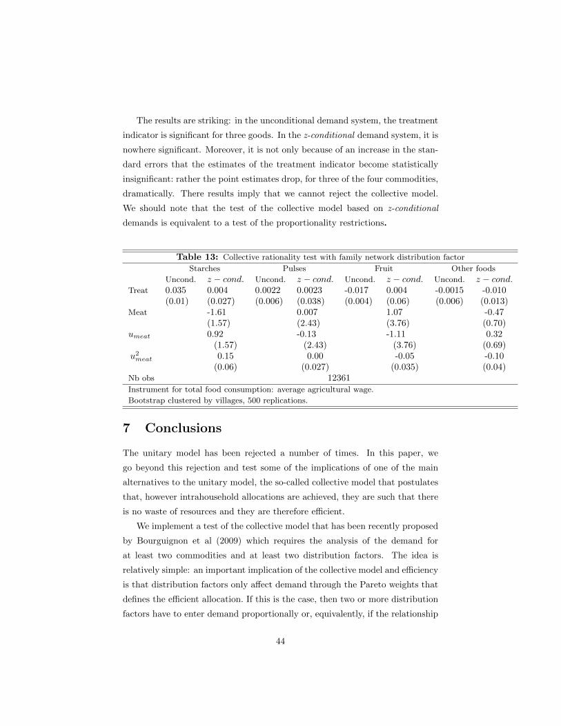
The results are striking: in the unconditional demand system, the treatment

indicator is significant for three goods. In the z-conditional demand system, it is

nowhere significant. Moreover, it is not only because of an increase in the stan-

dard errors that the estimates of the treatment indicator become statistically

insignificant: rather the point estimates drop, for three of the four commodities,

dramatically. There results imply that we cannot reject the collective model.

We should note that the test of the collective model based on z-conditional

demands is equivalent to a test of the proportionality restrictions.

Table 13: Collective rationality test with family network distribution factor

Starches Pulses Fruit Other foods

Uncond. z − cond. Uncond. z − cond. Uncond. z − cond. Uncond. z − cond.

Treat 0.035 0.004 0.0022 0.0023 -0.017 0.004 -0.0015 -0.010(0.01) (0.027) (0.006) (0.038) (0.004) (0.06) (0.006) (0.013)

Meat -1.61 0.007 1.07 -0.47(1.57) (2.43) (3.76) (0.70)

umeat 0.92 -0.13 -1.11 0.32(1.57) (2.43) (3.76) (0.69)

u2meat 0.15 0.00 -0.05 -0.10(0.06) (0.027) (0.035) (0.04)

Nb obs 12361Instrument for total food consumption: average agricultural wage.

Bootstrap clustered by villages, 500 replications.

7 Conclusions

The unitary model has been rejected a number of times. In this paper, we

go beyond this rejection and test some of the implications of one of the main

alternatives to the unitary model, the so-called collective model that postulates

that, however intrahousehold allocations are achieved, they are such that there

is no waste of resources and they are therefore efficient.

We implement a test of the collective model that has been recently proposed

by Bourguignon et al (2009) which requires the analysis of the demand for

at least two commodities and at least two distribution factors. The idea is

relatively simple: an important implication of the collective model and efficiency

is that distribution factors only affect demand through the Pareto weights that

defines the efficient allocation. If this is the case, then two or more distribution

factors have to enter demand proportionally or, equivalently, if the relationship

44

between the demand for one good and a distribution factor is monotonic, one can

condition on that commodity and ’explain away’ all other distribution factors.

We apply this test to the context of rural Mexico, on the data set collected

to evaluate the conditional cash transfer program PROGRESA. This data set is

ideal for a variety of reasons. First, the programme is targeted to women with

the explicit purpose of changing the balance of power within the households

that receive it. The programme itself, whose allocation is randomized across

localities within the evaluation sample, is an ideal distribution factor. Second,

the fact that the evaluation factor is a census within each village gives us the

opportunity to map out the family network and allows us to construct an addi-

tional distribution factor, the relative size of husband and wife family networks.

This measure is continuous and turns out to be an important determinant of

the demand for food.

We use the PROGRESA data to estimate a state of the art demand system

both with and without distribution factors. We first confirm that the demand

system we estimate without distribution factors is not stable and is unable to

predict the impact of the programme on consumption shares. The distribution

factors we consider are not only significant, but enter in a fashion which is not

inconsistent with the implications of the collective model. Moreover, we are

able, with these distribution factors, to predict the impacts of the programme

much better than the standard unitary model.

In the process of testing the collective model, our results also offer an ex-

planation for a phenomenon that has been observed in the context of a number

of conditional cash transfer programs, namely the fact that in the face of the

large change in total consumption that follows the injection of cash implied by

these programs, the structure of consumption, that is how total consumption is

allocated to different commodities, changes in ways that are hard to reconcile

with perceived wisdom or even with estimates of state of the art unitary demand

systems. We suggest that this might be due to a violation of the unitary model

and to the fact that the cash transfers delivered by these programmes are tar-

geted to women. Furthermore, we show that the deviations from the standard

model are not inconsistent with the collective model.

Our results are important because they constitute the first test of this na-

ture of the collective model in a context where the intrahousehold allocation

45

of resources is especially salient, as witnessed by the government’s attempt to

change it. Moreover, the fact that we do not reject the implications of the collec-

tive model is important because it points to a specific model of intrahousehold

resources that can be used to study household behaviour and establish the con-

sequences of different policies.

There are two parts to our approach to ‘test’ of the collective model. First,

we show how that, unlike a unitary model, the collective model, once we consider

explicitly the two distribution factors that we described (and, obviously, in

particular the first one) can predict the impact of PROGRESA upon budget

shares. Of course the impacts will be estimated with some error and one may

argue that the failure to reject the collective model is a lack of power that

comes both from the imprecision of the impact estimates and the imprecision

with which we estimate the model’s coefficients.

The second part of our approach takes a different tack and constitutes very

powerful evidence in favour of the collective model. We start from a rejection:

the fact that the coefficient on the PROGRESA indicator is strongly significant

while (within the unitary model) it should not be. This effect is strong and it

has been documented in many papers, both by us and others (see, for instance,

Schady and Rosero (2008), and Angelucci and Attanasio (2012)). Conditional

cash transfers targeted to women seem to shift Engel curves (rather than caus-

ing a movement in the demand of different commodities along an Engel curve).

We show that within the framework of the z − conditional demands that use

a distribution factor completely unrelated to PROGRESA (the relative size of

spouses networks), we can explain this shift. In other words, the test of Bour-

guignon et al. (2009) which we implement and that uses the second distribution

factor to construct the z − conditional demands is able to account for the shift

in Engel curves induced by the program. The coefficient on PROGRESA does

not just become insignificant, but it goes down in size. That is, by considering

the conditional demand system we are not just adding noise, we are actually

explaining the shift in the Engel curves.

Notice that the consideration of two distribution factors is crucial for our

analysis. If PROGRESA was the only distribution factor, we could not go

further than the rejection of the unitary model and the collective model would

saturate the data. Instead we are testing the hypothesis that under the collective

46

model all distribution factors are channelled through a unique index (the Pareto

weight or the sharing rule). This imposes a considerable amount of structure on

the data and could in principle be rejected.Traditional household surveys might

not contain information on distribution factors, so that it might not be possible,

in general, to replicate the exercise we are able to conduct here. We show that,

in our data where information on two plausible distribution factors is available

, the collective model cannot be rejected, while the unitary model is. Therefore,

the value of the exercise is to highlight the need for a representation of household

behaviour that allows for negotiation, and even possibly conflicting objectives;

as well as the need for different data, capturing exogenous variation in variables

that determine the relative power within the household. In future work, we plan

to test additional restrictions of the collective model, and in particular those on

the demand price elasticities.

References

[1] Altonji, J.G., Hayashi, F.and L.J. Kotlikoff, (1992): ”Is the extended familyaltruistically linked? Direct tests using micro data.” American EconomicReview 85, 1177–1198.

[2] Altonji, J.G., Hayashi, F.and L.J. Kotlikoff, (1997). ”Parental altruism andinter vivos transfers: theory and evidence.” Journal of Political Economy105, 1121–1166.

[3] Angelucci, M. and O. Attanasio, (2009), ”Oportunidades: programme ef-fects on consumption, low participation, and methodological issues”, Eco-nomic Development and Cultural Change, Vol. 57, pp.479-506.

[4] Angelucci, M. and O. Attanasio, (2012), ”The Demand for Food of Poor Ur-ban Mexican Households: Understanding Policy Impacts Using structuralModels”, forthcoming in American Economic Journal: Economic Policy.

[5] Angelucci, M., De Giorgi, (2009), ”Indirect Effects of an Aid Program: Howdo Cash Transfers Affect Ineligibles’Consumption”, American EconomicReview, vol99(1), page 486-508.

[6] Angelucci, M., De Giorgi, G., Rangel, M. and I.Rasul, 2009. ”VillageEconomies and the Structure of Extended Family Networks,” The B.E.Journal of Economic Analysis & Policy, De Gruyter, vol. 9(1), pages 44.

[7] Attanasio, O.P., Battistin, E. and A. Mesnard (2012): ”Food and CashTransfers: Evidence from Colombia,” Economic Journal, Royal EconomicSociety, vol. 122, pp. 92-124.

[8] Attanasio, O.P. and V. Lechene (2002), ”Tests of Income Pooling in House-hold Decisions”, Review of Economic Dynamics, Vol. 5, pp. 720-748.

[9] Attanasio, O.P. and V. Lechene (2010), “Conditional Cash Transfers,Women and the Demand for Food”, IFS Working Paper 10/17.

47

[10] Attanasio, O.P., Di Maro V., Lechene V and D. Phillips,(2009) ”The welfareconsequence of increases in food prices in rural Mexico and Colombia”, IFSWorking Paper.

[11] Attanasio, O.P., Di Maro V., Lechene V and D. Phillips, (2013) ”The effectof increases in food prices on consumption and welfare in rural Mexico”,forthcoming, Journal of Development Economics.

[12] Banks, J., Blundell, R. and A. Lewbel, (1997). ”Quadratic Engel CurvesAnd Consumer Demand,” The Review of Economics and Statistics, MITPress, vol. 79(4), pages 527-539, November.

[13] Behrman, J.R. and M. Rosenzweig, (2006): ”Parental wealth and adultchildren’s welfare in marriage.” Review of Economics and Statistics 88,496–509.

[14] Behrman, J.R., and Todd, P.,(1999): ”Randomness in the Ex-perimental Samples of PROGRESA”, IFPRI Working Paper,http://www.ifpri.org/sites/default/files/publications/behrmantodd random.pdf.

[15] Bobonis, G. (2009): ”Is the Allocation of Resources within the HouseholdEfficient? New Evidence from a Randomized Experiment”, Journal of Po-litical Economy, vol. 117, pp. 453-503.

[16] Bourguignon, F., Browning, M. and P.A. Chiappori (2009) “Efficient Intra-Household Allocations and Distribution Factors: Implication and Identifi-cation ”, Review of Economic Studies, 76, pp 503-28.

[17] Bourguignon, F., Browning, M., Chiappori P.A. and V. Lechene, (1993),“Intra-Household Allocation of Consumption: A Model and Some Evidencefrom French Data”, Annales d’Economie et de Statistiques, n29, Janvier-Mars 1993, p137-157.

[18] Browning, M., Bourguignon F., Chiappori P.A., and V.Lechene, (1994),”Incomes and Outcomes: A Structural Model of Intra-Household Allo-cation”, Journal of Political Economy, University of Chicago Press, vol.102(6), pages 1067-96, December.

[19] Browning, M., Chiappori, P-A., (1998): ”Efficient Intra-Household Alloca-tions: A General Characterization and Empirical Tests” Econometrica, 66,pp.1241-1278.

[20] Browning, M., Chiappori, P-A., Lechene, V., (2006), ”Collective and uni-tary models: a clarification”, Review of Economic of the Household.

[21] Browning, M., and C. Meghir (1991), ”The effect of Male and Female LaborSupply on Commodity Demands”, Econometrica, 59, pp.925-951.

[22] Chiappori, P.A. (1988)”Rational Household Labor Supply”, Econometrica,56, 1988, 63-89.

[23] Chiappori, P.A. (1992)”Collective labor supply and welfare”, Journal ofPolitical Economy, 100, 1992, 437-67.

[24] Cox, D. and G. Jakubson, (1995): ”The connection between public transfersand private interfamily transfers.” Journal of Public Economics 57, 129–167.

48

[25] Cox, D.and M. Fafchamps, (2008): ”Extended Family and Kinship Net-works: Economic Insights and Evolutionary Directions”. In: T.P. Schultz,J.A. Strauss (Eds.), Chapter 58 in Handbook of Development EconomicsVol. 4, Elsevier, pp. 3711–384

[26] Deaton, A., and Muellbauer, J., (1980), ”An Almost Ideal Demand Sys-tem,” American Economic Review, American Economic Association, vol.70(3), pages 312-26, June.

[27] Fiszbein A. and N. Schady (2009) Conditional Cash Transfers: Reduc-ing Present and Future Poverty World Bank Policy Research Report, TheWorld Bank, Washington.

[28] Gertler, P. Martinez, S. and M. Rubio-Codina (2012): ”Investing CashTransfers to Raise Long-Term Living Standards,” American EconomicJournal: Applied Economics, 4, 164-92.

[29] Hoddinot, J., and Skoufias, E., (2004), ”The Impact of PROGRESA onFood Consumption,” Economic Development and Cultural Change, Uni-versity of Chicago Press, vol. 53(1), pages 37-61, October.

[30] IFPRI (2006): ”PROGRESA”, http://www.ifpri.org/book-766/ourwork/program/progresa

[31] La Ferrara, E., (2003): ”Kin groups and reciprocity: a model of credittransactions in Ghana.” American Economic Review 93, 1730–1751.

[32] Loury, L.D., (2006): ”All in the extended family: effects of grandparents,aunts, and uncles on educational attainment.” American Economic ReviewPapers and Proceedings 96, 275–278.

[33] Procidano, M.E. and K. Heller (1983): ”Measures of perceived social sup-port from friends and from family: Three validation studies.” AmericanJournal of Community Psychology, 11, 1-24.

[34] Riccio, J. Dechausay, N, Greenberg, D. Miller ,C., Rucks, Z and N.Verma(2010):”Toward Reduced Poverty Across Generations. Early Find-ings from New York City’s Conditional Cash Transfer Program ”MDRCreport, http://www.mdrc.org/sites/default/files/full 588.pdf.

[35] Rosenzweig, M.R., (1988): ”Risk, implicit contracts and the family in ruralareas of low income countries.” Economic Journal 98, 1148–1170.

[36] Rosenzweig, M.R. and O. Stark (1989): ”Consumption smoothing, Migra-tion and Marriage: Evidence from Rural India. Journal of Political Econ-omy, 97, 905-926.

[37] Schady, N. and J. Rosero ( 2008): ”Are cash transfers made to womenspent like other sources of income?,” Economics Letters, 101, 246-248.

[38] Schultz, T.P., 2004. School subsidies for the poor: evaluating the Mex-ican PROGRESA Poverty Program. Journal of Development Economics74, 199–250.

[39] Skoufias, E. (2001): ”PROGRESA and its impacts on the human capitaland welfare of households in rural Mexico”, International Food Policy Re-search Institute (IFPRI), http://www.ifpri.org/publication/progresa-and-its-impacts-human-capital-and-welfare-households-rural-mexico

49

[40] Skoufias E. and V. Di Maro, (2008): ”Conditional Cash Transfers, AdultWork Incentives, and Poverty,” Journal of Development Studies, 44, 935-960.

[41] Skoufias, E., Mcclafferty, B., 2001. Is PROGRESA working? Summary ofthe results of an evaluation by IFPRI. FCND Discussion Paper No.118.

[42] Skoufias, E., Parker, S., 2001. Conditional cash transfers and their impacton child work and schooling: evidence from the PROGRESA program inMexico. Economia 2, 45–96.

[43] Weiss, Y. and R.J. Willis, R.J (1985): ”Children as collective goods anddivorce settlements.” Journal of Labor Economics 3, 268–292.

50