Last Modified 11/28/2014

III-1-1

III-1 Consequences of Flooding

Introduction

Flood water can be one of the most destructive forces on earth, especially if caused by an

event that unexpectedly overwhelms an existing flood defense 1or by catastrophic breach

of a dam or levee. Recent events, such as flooding caused by Hurricane Katrina and the

tsunami in Japan, have caused thousands of people to lose their life and unknown billions

of dollars in damages. By the same token, dozens of floods (some from similarly

unexpected events like a dam or levee breach) occur every year with no resulting loss of

life and relatively minimal property damage.

Although flooding can have many types of severe consequences, including economic,

social, cultural, and environmental, the primary objective of Reclamation’s dam safety

program and USACE’s dam and levee safety programs are to manage the risk to the

public who rely on those structures, and to keep them reasonably safe from flooding.

Thus, reducing the risk associated with loss of life is paramount. The safety programs of

both agencies treat life loss separately from economic and other considerations.

Decisions as to whether invest in dam or levee improvements are based primarily on risk

to life by applying the concept of tolerable risks. Since informed decisions based on

tolerable risk require estimates of loss of life for potential flood events, the focus of this

chapter is on estimating loss of life. Estimation of the magnitude of life loss resulting

from a flood requires consideration of the following factors:

Understanding of the population at risk in the potentially impacted area

Warning and evacuation assumptions for that population at risk

Flood characteristics including extents, depths, velocities, and arrival time (can

be heavily influence by failure mode and breach parameters)

Estimation of fatality rates

The full consideration of all these factors is a complex problem that requires detailed

modeling of the physical processes (breach characteristics and flood routing), human

responses, and the performance of technological systems (such as warning and

evacuation systems, transportation systems and buildings under flood loading). This

chapter describes a range of practical approaches to this complex problem that can

provide life-loss estimates for use in risk analysis.

Consequences Methodologies and Perspectives –

USACE and Reclamation

Both the U.S. Army Corps of Engineers (USACE) and the Bureau of Reclamation

(Reclamation) perform risk analysis for the dams or levees (USACE only) to assist with

risk informed decision making on flood defense infrastructure within each agency’s

portfolio. While the basic concept of using life loss estimates to help quantify risk is

similar between each agencies, the methodologies employed by the two agencies have

differences. This consequences estimation chapter is intended for use by both agencies,

III-1-2

and is structured in a way that presents general information on life loss estimation,

followed by agency-specific subsections.

Life loss estimation models currently in use by USACE include the LifeSim model and

HEC-FIA, which contains a simplified version of LifeSim. Importantly, since the

simplified LifeSim methodology in HEC-FIA is derived from the LifeSim approach, a

specific application of HEC-FIA can be scaled up to a full LifeSim application by

developing and gathering the necessary supplemental data.

LifeSim is an agent-based simulation model that tracks the movement of people and their

interaction with flooding through time. It includes an integrated transportation algorithm

to model the evacuation process, and evaluates loss of life based on location of people

when the water arrives and important factors related to building, vehicle, and human

stability. Fatalities are estimated by grouping people into one of three “zones”. Each zone

has a corresponding fatality rate, which were developed based on an extensive review and

analysis of historic flood events.

HEC-FIA includes a simplified version of the LifeSim methodology. Applicability of

HEC-FIA depends on the goals of the assessment as well as the characteristics of the

study area. The main differences between the simplified LifeSim methodology applied

within HEC-FIA and the ful LifeSim methodology include simplifying assumptions

related to evacuation simulation and how flood wave arrival times are determined.

Grouping of persons into zones and application of fatality rates is similar to the full

LifeSim model. More details on the difference between LifeSim and HEC-FIA life loss

methodologies are described in the USACE Loss of Life Estimation Methodology section

later in this chapter.

Prior to 2014, Reclamation used the DSO-99-06 method for the vast majority of life loss

assessments. Beginning in 2014, Reclamation Consequence Estimating Methodology

(RCEM) replaced DSO-99-06 as the standard life loss estimating methodology. Both

RCEM and DSO-99-06 are based on case history data and judgment. Fatality rates are

developed using key parameters including warning time and flood severity. RCEM is

relatively simple to apply but requires more judgment than DSO-99-06.

Reclamation has also been developing capability with the Life Safety Model. Similar to

the LifeSim model used by USACE, the Life Safety Model is a simulation model that

tracks movement of water and movement of people. Fatalities are estimated based on

various factors including building destruction, vehicle toppling and drowning. The Life

Safety Model has an integrated transportation model, but does not use empirical-based

fatality rates.

Summary of Historic Flooding Events

In order to understand the potential for loss of life from flooding and the strengths and

weaknesses of the available life loss methodologies, it is important to understand what

has lead to loss of life during flood events in the past. All flood disasters are unique in

many ways. However, there are a few commonalities that are consistent across most

flood scenarios when it comes to how many people lose their life. These common factors

include the intensity of the flooding and the time available for warning and evacuation.

This section summarizes several historic flood disasters and describes the driving factors

that influenced the loss of life for each scenario. Many of these events were used to

III-1-3

inform the fatality rates used in LifeSim, FIA, and RCEM. As part of the RCEM, the

Dam Failure and Flood Event Case History Compilation includes descriptions of about

60 historical events, with details of the population at risk, flood severity, warning and

fatalities.

Teton Dam Teton Dam, constructed, owned and operated by Reclamation, failed during first filling

on Saturday June 5, 1976. The dam was located on the Teton River, about three miles

northeast of the town of Newdale, Idaho. Teton Dam was an central-core, zoned

embankment dam with a 305 foot structural height (not including 100 feet of additional

foundation excavation), and contained 251,700 acre-feet of storage at the time of failure.

The cause of failure was internal erosion of the core of the dam, initiated within the

foundation key trench.

During the night of June 4, water evidently flowed down the right groin, and a shallow

damp channel was noticed early on the morning of June 5. Shortly after 7 a.m. on June 5,

muddy water was flowing at about 20 to 30 cubic feet per second from talus on the right

abutment. At about 10:30 a.m., a large leak of about 15 cubic feet per second appeared on

the face of the embankment, possibly associated with a “loud burst” heard at that time.

The new leak increased and appeared to emerge from a “tunnel” about 6 feet in diameter,

roughly perpendicular to the dam axis and extending at least 35 feet into the

embankment. The tunnel became an erosion gully developing headward up the

embankment and curving toward the abutment. At about 11 a.m., a vortex appeared in the

reservoir, above the upstream slope of the embankment. At 11:30 a.m., a small sinkhole

appeared temporarily, ahead of the gully developing on the downstream slope, near the

top of the dam. Shortly thereafter, at 11:57 a.m., the top of the dam collapsed and the

reservoir was breached.

Failure of the dam released 240,000 acre-feet in about six hours. Flooding reached the

town of Wilford, 8.4 miles downstream, within 30 minutes or so. Six fatalities occurred at

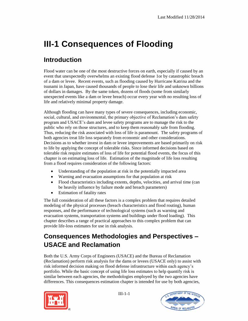
Wilford and 120 of 154 homes were swept away. Flooding 12.3 miles downstream at

Sugar City arrived at 1:30 pm and was described as a 15 foot high wall of water. At

Rexburg, 15.3 miles downstream, flooding arrived at 2:30 pm and reached a depth of 6 to

8 feet within minutes.

Eleven fatalities occurred as a result of the dam’s failure, although it is thought by some

that the consequences could have been much worse if the dam had failed at night with no

warning. Persons were present at the dam while it was failing and evacuation of

downstream population was ordered thirty minutes to an hour prior to the full

development of the breach. More than 30,000 people in total were evacuated. Some

fatalities occurred when persons who had previously evacuated went back into the flood

zone to retrieve possessions.

Out of the eleven fatalities, six died from drowning, three from heart attack, one from

accidental shooting and one from self inflicted gunshot wounds.

Maximum dam failure discharge was about 2.3 million ft3/s at Teton Canyon, 2.5 miles

downstream from the dam. At Wilford, the flood is estimated to have attenuated to

1,060,000 ft3/s.

III-1-4

Figure III-1-1. Teton Dam Failure

Figure III-1-2. Flooding and evacuation at Rexburg, Idaho

III-1-5

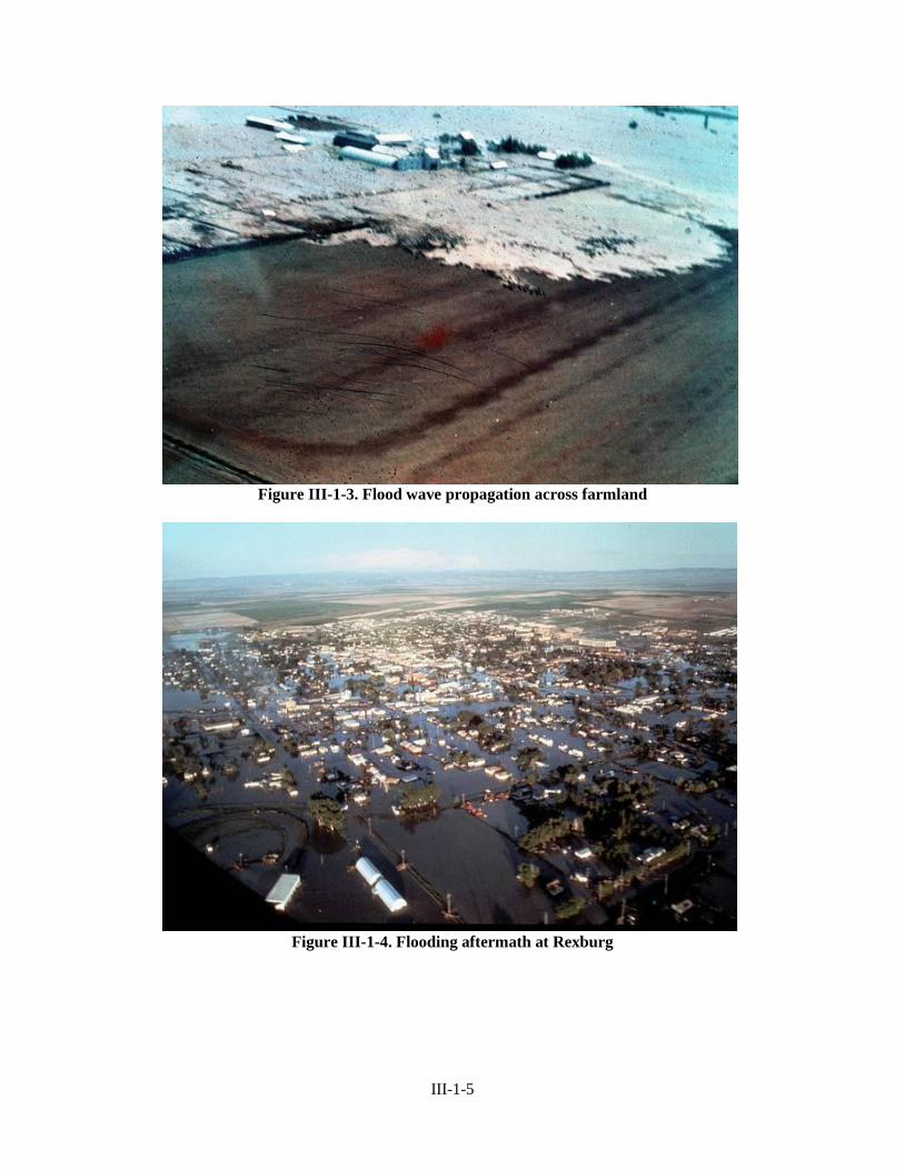
Figure III-1-3. Flood wave propagation across farmland

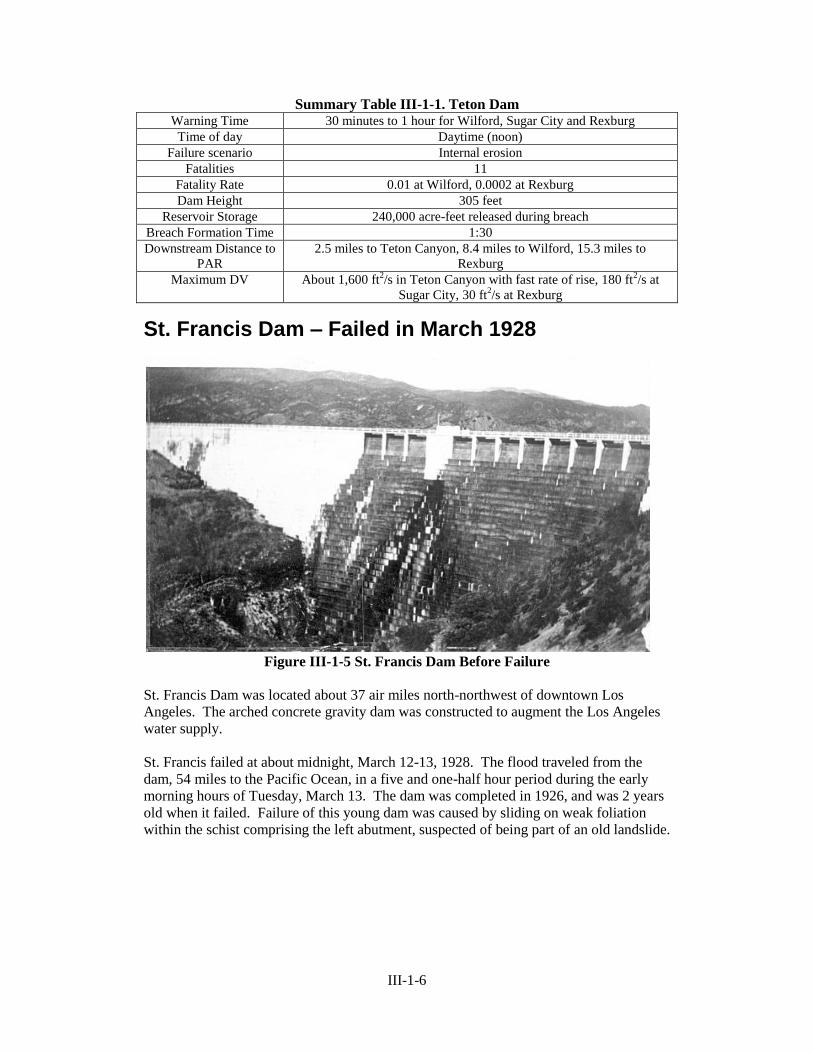
Figure III-1-4. Flooding aftermath at Rexburg

III-1-6

Summary Table III-1-1. Teton Dam Warning Time 30 minutes to 1 hour for Wilford, Sugar City and Rexburg

Time of day Daytime (noon)

Failure scenario Internal erosion

Fatalities 11

Fatality Rate 0.01 at Wilford, 0.0002 at Rexburg

Dam Height 305 feet

Reservoir Storage 240,000 acre-feet released during breach

Breach Formation Time 1:30

Downstream Distance to

PAR

2.5 miles to Teton Canyon, 8.4 miles to Wilford, 15.3 miles to

Rexburg

Maximum DV About 1,600 ft2/s in Teton Canyon with fast rate of rise, 180 ft

2/s at

Sugar City, 30 ft2/s at Rexburg

St. Francis Dam – Failed in March 1928

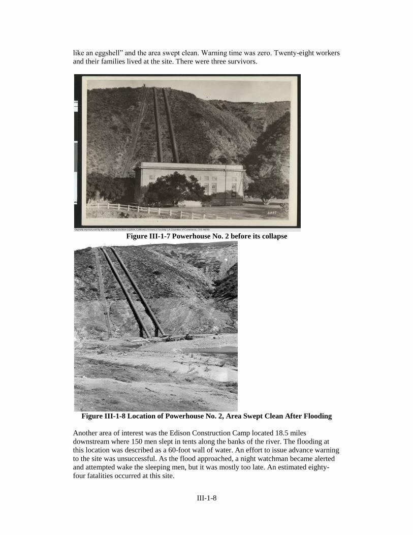
Figure III-1-5 St. Francis Dam Before Failure

St. Francis Dam was located about 37 air miles north-northwest of downtown Los

Angeles. The arched concrete gravity dam was constructed to augment the Los Angeles

water supply.

St. Francis failed at about midnight, March 12-13, 1928. The flood traveled from the

dam, 54 miles to the Pacific Ocean, in a five and one-half hour period during the early

morning hours of Tuesday, March 13. The dam was completed in 1926, and was 2 years

old when it failed. Failure of this young dam was caused by sliding on weak foliation

within the schist comprising the left abutment, suspected of being part of an old landslide.

III-1-7

Figure III-1-6 The Breached St. Francis Dam

St. Francis Dam had a height of 188 feet, and the reservoir volume at the time of failure

was about 38,000 acre-feet. The reservoir was about 3 feet below the crest of the parapet

at the initiation of dam failure.

The failure sequence for this dam can be considered a worst case scenario. Failure

occurred in the middle of the night when many people would have been asleep and

darkness prevented people from observing the events that were occurring. The dam

failed suddenly with no warning being issued before failure, and the entire contents of the

reservoir drained in less than 72 minutes. The dam tender was unable to alert anyone of

the danger. He and his family lived in the valley downstream from the dam and perished

in the flood.

The Ventura County Sheriff’s Office was informed at 1:20 a.m. Telephone operators

called local police, highway patrol and phone company customers. Warning was spread

by word of mouth, phone, siren and law enforcement in motor vehicles.

Flooding was severe through a 54-mile reach from the dam to the ocean. The leading

edge of the flooding moved at about 18 miles per hour near the dam and 6 miles per hour

closer to the ocean. There were about 3,000 people at risk and about 420 fatalities,

although the number of fatalities reported varies significantly. The fatality rate for the

entire reach was about 0.14. It was much higher than this near the dam and much lower

as the flood approached the Pacific Ocean. The dam was not rebuilt.

Two downstream areas, Powerhouse No. 2 and Edison Construction Camp, are of

particular interest when it comes to understanding how the severity of flooding resulting

from this breach lead to relatively high loss of life.

The Powerhouse No. 2 located in the San Francisquito Canyon, about 1.4 miles

downstream from the dam. The flood arrived at this location as a wall of water, about five

minutes after the dam had failed with an estimated maximum flood depth of 120 feet and

peak discharge of 1.3 million ft3/s. The 60-foot tall concrete powerhouse was “crushed

III-1-8

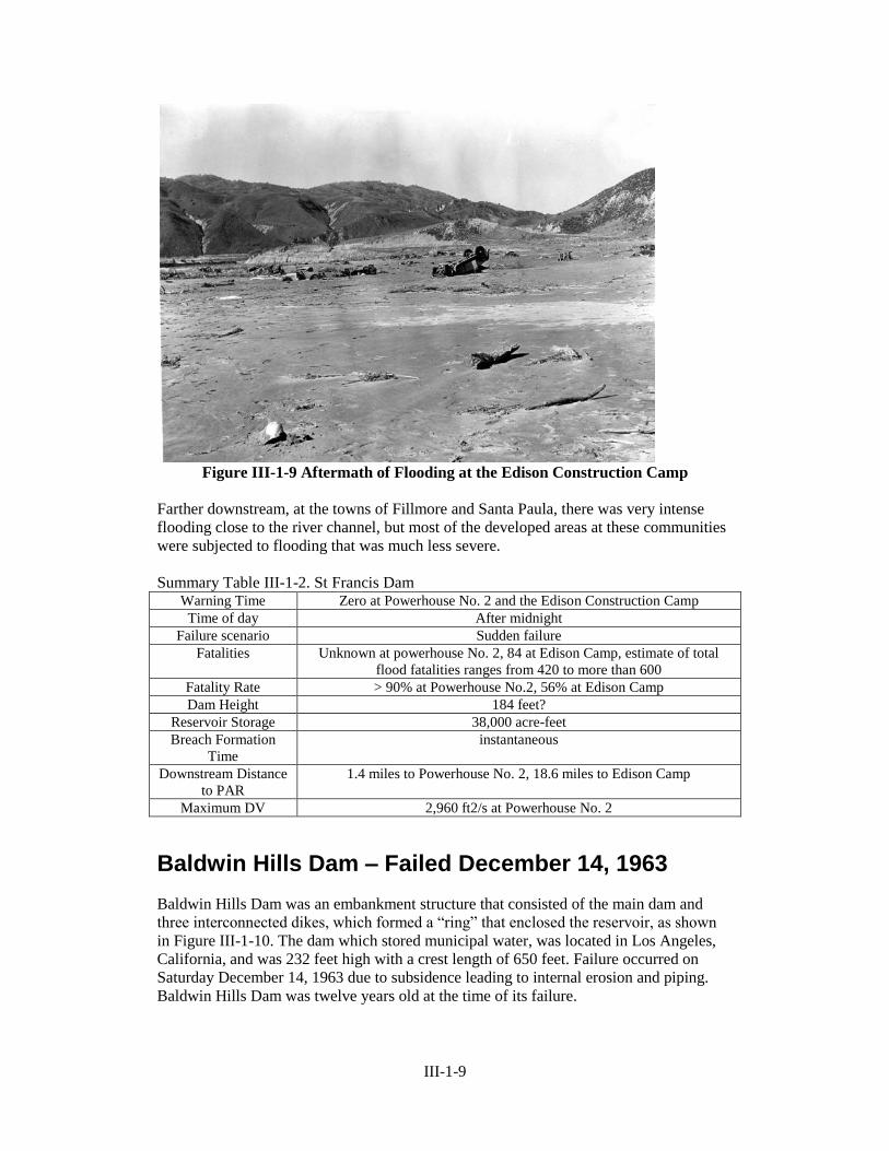
like an eggshell” and the area swept clean. Warning time was zero. Twenty-eight workers

and their families lived at the site. There were three survivors.

Figure III-1-7 Powerhouse No. 2 before its collapse

Figure III-1-8 Location of Powerhouse No. 2, Area Swept Clean After Flooding

Another area of interest was the Edison Construction Camp located 18.5 miles

downstream where 150 men slept in tents along the banks of the river. The flooding at

this location was described as a 60-foot wall of water. An effort to issue advance warning

to the site was unsuccessful. As the flood approached, a night watchman became alerted

and attempted wake the sleeping men, but it was mostly too late. An estimated eighty-

four fatalities occurred at this site.

III-1-9

Figure III-1-9 Aftermath of Flooding at the Edison Construction Camp

Farther downstream, at the towns of Fillmore and Santa Paula, there was very intense

flooding close to the river channel, but most of the developed areas at these communities

were subjected to flooding that was much less severe.

Summary Table III-1-2. St Francis Dam Warning Time Zero at Powerhouse No. 2 and the Edison Construction Camp

Time of day After midnight

Failure scenario Sudden failure

Fatalities Unknown at powerhouse No. 2, 84 at Edison Camp, estimate of total

flood fatalities ranges from 420 to more than 600

Fatality Rate > 90% at Powerhouse No.2, 56% at Edison Camp

Dam Height 184 feet?

Reservoir Storage 38,000 acre-feet

Breach Formation

Time

instantaneous

Downstream Distance

to PAR

1.4 miles to Powerhouse No. 2, 18.6 miles to Edison Camp

Maximum DV 2,960 ft2/s at Powerhouse No. 2

Baldwin Hills Dam – Failed December 14, 1963

Baldwin Hills Dam was an embankment structure that consisted of the main dam and

three interconnected dikes, which formed a “ring” that enclosed the reservoir, as shown

in Figure III-1-10. The dam which stored municipal water, was located in Los Angeles,

California, and was 232 feet high with a crest length of 650 feet. Failure occurred on

Saturday December 14, 1963 due to subsidence leading to internal erosion and piping.

Baldwin Hills Dam was twelve years old at the time of its failure.

III-1-10

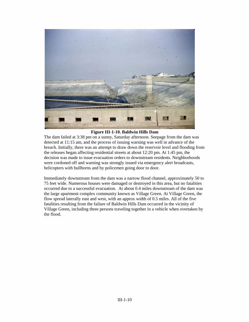
Figure III-1-10. Baldwin Hills Dam

The dam failed at 3:38 pm on a sunny, Saturday afternoon. Seepage from the dam was

detected at 11:15 am, and the process of issuing warning was well in advance of the

breach. Initially, there was an attempt to draw down the reservoir level and flooding from

the releases began affecting residential streets at about 12:20 pm. At 1:45 pm, the

decision was made to issue evacuation orders to downstream residents. Neighborhoods

were cordoned off and warning was strongly issued via emergency alert broadcasts,

helicopters with bullhorns and by policemen going door to door.

Immediately downstream from the dam was a narrow flood channel, approximately 50 to

75 feet wide. Numerous houses were damaged or destroyed in this area, but no fatalities

occurred due to a successful evacuation. At about 0.4 miles downstream of the dam was

the large apartment complex community known as Village Green. At Village Green, the

flow spread laterally east and west, with an approx width of 0.5 miles. All of the five

fatalities resulting from the failure of Baldwin Hills Dam occurred in the vicinity of

Village Green, including three persons traveling together in a vehicle when overtaken by

the flood.

III-1-11

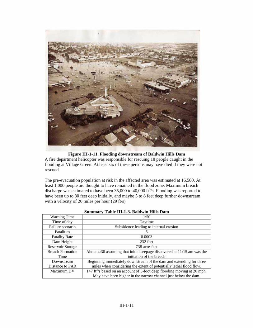
Figure III-1-11. Flooding downstream of Baldwin Hills Dam

A fire department helicopter was responsible for rescuing 18 people caught in the

flooding at Village Green. At least six of these persons may have died if they were not

rescued.

The pre-evacuation population at risk in the affected area was estimated at 16,500. At

least 1,000 people are thought to have remained in the flood zone. Maximum breach

discharge was estimated to have been 35,000 to 40,000 ft3/s. Flooding was reported to

have been up to 30 feet deep initially, and maybe 5 to 8 feet deep further downstream

with a velocity of 20 miles per hour (29 ft/s).

Summary Table III-1-3. Baldwin Hills Dam Warning Time 1:50

Time of day Daytime

Failure scenario Subsidence leading to internal erosion

Fatalities 5

Fatality Rate 0.0003

Dam Height 232 feet

Reservoir Storage 738 acre-feet

Breach Formation

Time

About 4:30 assuming that initial seepage discovered at 11:15 am was the

initiation of the breach

Downstream

Distance to PAR

Beginning immediately downstream of the dam and extending for three

miles when considering the extent of potentially lethal flood flow.

Maximum DV 147 ft2/s based on an account of 5-foot deep flooding moving at 20 mph.

May have been higher in the narrow channel just below the dam.

III-1-12

Damage in the Village Green area was extensive, but many structures remained standing

after the flood. The narrow flood channel immediately downstream of the dam

experienced high intensity flooding, although no fatalities occurred in this area.

Laurel Run Dam – July 20, 1977

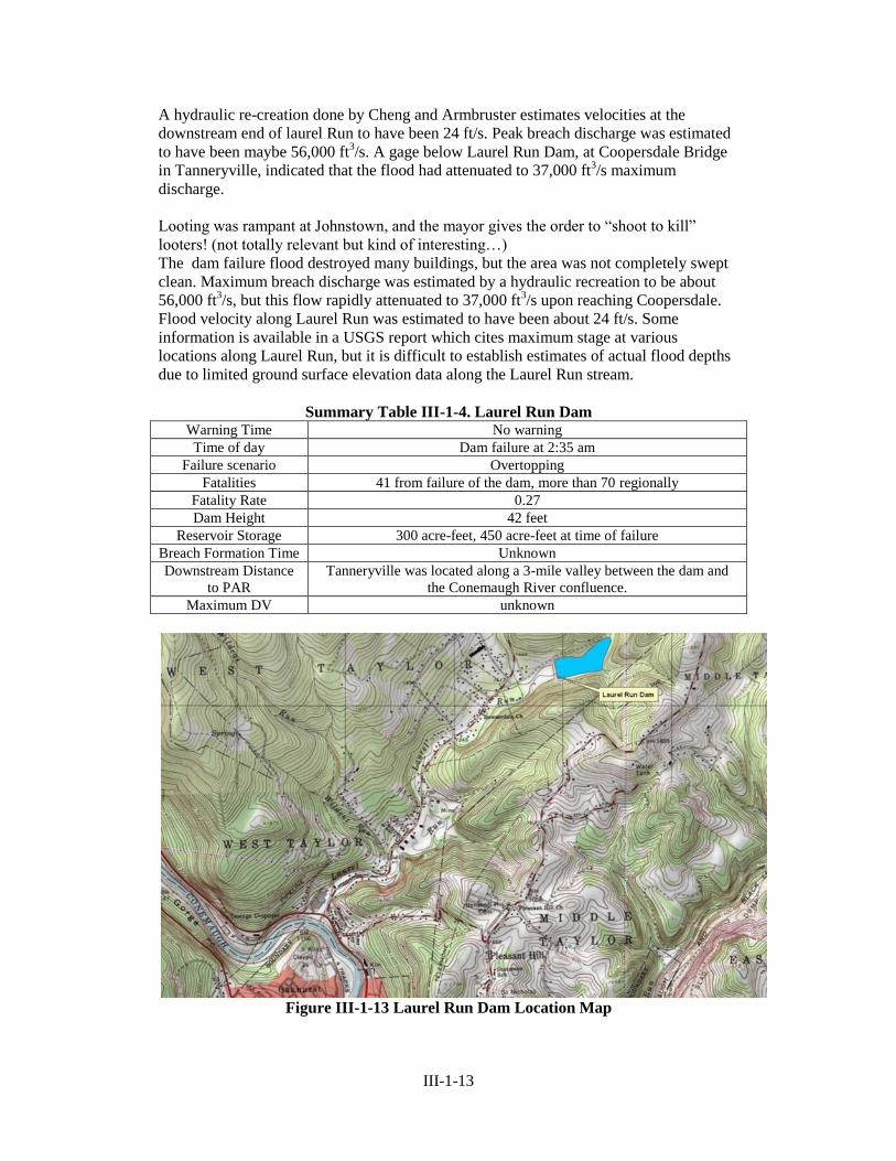
Laurel Run Dam was located on a stream known as Laurel Run located in west-central

Pennsylvania, near the town of Johnstown. The earthen dam was 42 feet high with a 623

foot crest length and the reservoir typically held about 300 acre-feet of storage. 450 acre-

feet of storage was reported to be in the reservoir at the time of its failure.

Laurel Run had the largest reservoir of seven dams to fail between July 19 and 20, 1977

and caused the most fatalities from this event. The dam is claimed to have failed at 2:35

am on morning of July 20 after a period of heavy rain. 11.82 inches of rain fell in 10

hours, and this was estimated to be between a 5,000 to 10,000 year rainfall event. The

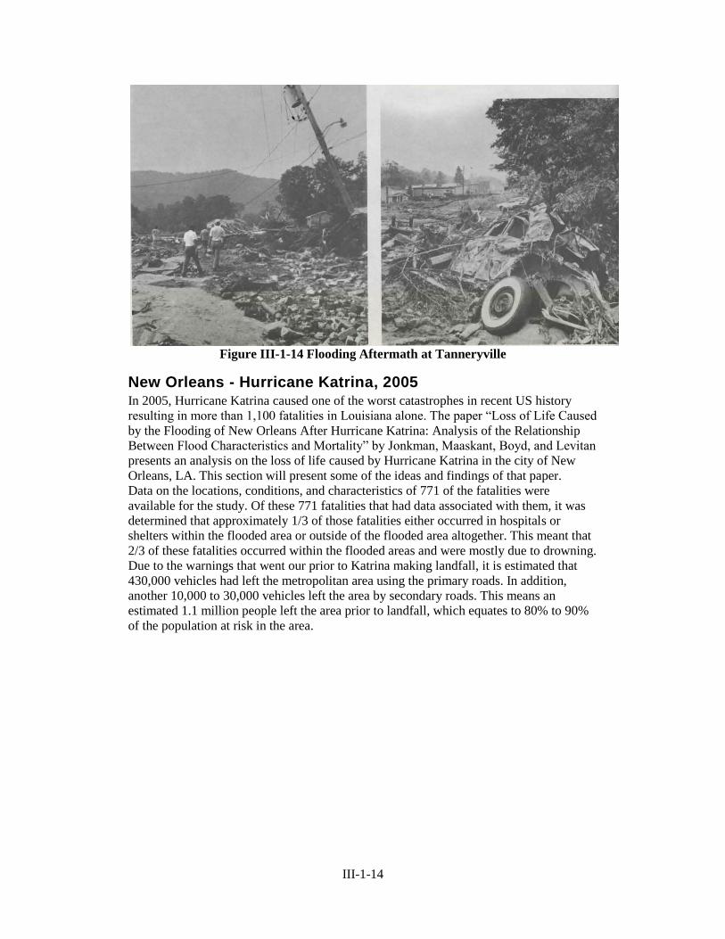
dam failed from overtopping. About 41 people were killed in the town of Tanneryville,

located in a three-mile long valley, immediately downstream of the dam. Most residents

were asleep when the dam failed and no warning was issued. In addition, the rain and

night-time conditions limited any escape. Many of the homes in Tanneryville were either

damaged or destroyed.

Figure III-1-12 Remains of Laurel Run Dam

Another dam, Sandy Run Dam, was also responsible for several deaths. Overall, there

were more than 70 deaths in the area resulting from the effects of this regional flood. The

town of Johnstown along the Conemaugh River, famous for the flooding from the 1889

failure of South Fork Dam, was heavily flooded. Damage to Johnstown was extensive,

but without fatalities. The area experienced widespread power outages the night of the

flood. Telephone service was intermittent in some communities as well. Laurel Run Dam

was not rebuilt.

III-1-13

A hydraulic re-creation done by Cheng and Armbruster estimates velocities at the

downstream end of laurel Run to have been 24 ft/s. Peak breach discharge was estimated

to have been maybe 56,000 ft3/s. A gage below Laurel Run Dam, at Coopersdale Bridge

in Tanneryville, indicated that the flood had attenuated to 37,000 ft3/s maximum

discharge.

Looting was rampant at Johnstown, and the mayor gives the order to “shoot to kill”

looters! (not totally relevant but kind of interesting…)

The dam failure flood destroyed many buildings, but the area was not completely swept

clean. Maximum breach discharge was estimated by a hydraulic recreation to be about

56,000 ft3/s, but this flow rapidly attenuated to 37,000 ft

3/s upon reaching Coopersdale.

Flood velocity along Laurel Run was estimated to have been about 24 ft/s. Some

information is available in a USGS report which cites maximum stage at various

locations along Laurel Run, but it is difficult to establish estimates of actual flood depths

due to limited ground surface elevation data along the Laurel Run stream.

Summary Table III-1-4. Laurel Run Dam Warning Time No warning

Time of day Dam failure at 2:35 am

Failure scenario Overtopping

Fatalities 41 from failure of the dam, more than 70 regionally

Fatality Rate 0.27

Dam Height 42 feet

Reservoir Storage 300 acre-feet, 450 acre-feet at time of failure

Breach Formation Time Unknown

Downstream Distance

to PAR

Tanneryville was located along a 3-mile valley between the dam and

the Conemaugh River confluence.

Maximum DV unknown

Figure III-1-13 Laurel Run Dam Location Map

III-1-14

Figure III-1-14 Flooding Aftermath at Tanneryville

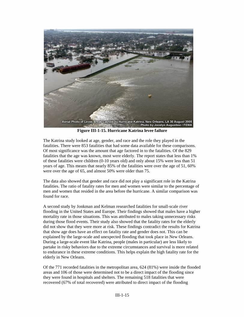
New Orleans - Hurricane Katrina, 2005 In 2005, Hurricane Katrina caused one of the worst catastrophes in recent US history

resulting in more than 1,100 fatalities in Louisiana alone. The paper “Loss of Life Caused

by the Flooding of New Orleans After Hurricane Katrina: Analysis of the Relationship

Between Flood Characteristics and Mortality” by Jonkman, Maaskant, Boyd, and Levitan

presents an analysis on the loss of life caused by Hurricane Katrina in the city of New

Orleans, LA. This section will present some of the ideas and findings of that paper.

Data on the locations, conditions, and characteristics of 771 of the fatalities were

available for the study. Of these 771 fatalities that had data associated with them, it was

determined that approximately 1/3 of those fatalities either occurred in hospitals or

shelters within the flooded area or outside of the flooded area altogether. This meant that

2/3 of these fatalities occurred within the flooded areas and were mostly due to drowning.

Due to the warnings that went our prior to Katrina making landfall, it is estimated that

430,000 vehicles had left the metropolitan area using the primary roads. In addition,

another 10,000 to 30,000 vehicles left the area by secondary roads. This means an

estimated 1.1 million people left the area prior to landfall, which equates to 80% to 90%

of the population at risk in the area.

III-1-15

Figure III-1-15. Hurricane Katrina levee failure

The Katrina study looked at age, gender, and race and the role they played in the

fatalities. There were 853 fatalities that had some data available for these comparisons.

Of most significance was the amount that age factored in to the fatalities. Of the 829

fatalities that the age was known, most were elderly. The report states that less than 1%

of these fatalities were children (0-10 years old) and only about 15% were less than 51

years of age. This means that nearly 85% of the fatalities were over the age of 51, 60%

were over the age of 65, and almost 50% were older than 75.

The data also showed that gender and race did not play a significant role in the Katrina

fatalities. The ratio of fatality rates for men and women were similar to the percentage of

men and women that resided in the area before the hurricane. A similar comparison was

found for race.

A second study by Jonkman and Kelman researched fatalities for small-scale river

flooding in the United States and Europe. Their findings showed that males have a higher

mortality rate in those situations. This was attributed to males taking unnecessary risks

during those flood events. Their study also showed that the fatality rates for the elderly

did not show that they were more at risk. These findings contradict the results for Katrina

that show age does have an effect on fatality rate and gender does not. This can be

explained by the large-scale and unexpected flooding that took place in New Orleans.

During a large-scale event like Katrina, people (males in particular) are less likely to

partake in risky behaviors due to the extreme circumstances and survival is more related

to endurance in these extreme conditions. This helps explain the high fatality rate for the

elderly in New Orleans.

Of the 771 recorded fatalities in the metropolitan area, 624 (81%) were inside the flooded

areas and 106 of those were determined not to be a direct impact of the flooding since

they were found in hospitals and shelters. The remaining 518 fatalities that were

recovered (67% of total recovered) were attributed to direct impact of the flooding

III-1-16

(drowning, physical trauma, or building collapse). Of these fatalities, it was determined

that many were near large breaches in the levees and therefore, were in areas that

experienced deeper water levels.

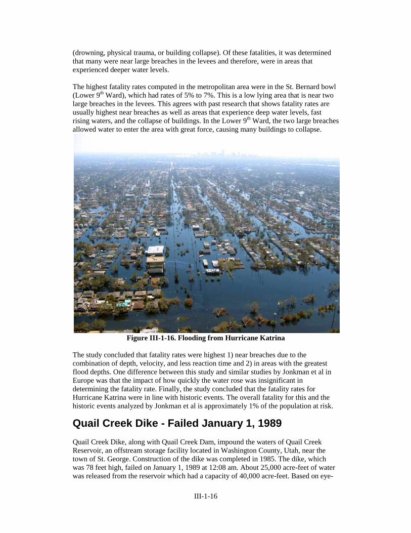
The highest fatality rates computed in the metropolitan area were in the St. Bernard bowl

(Lower 9th Ward), which had rates of 5% to 7%. This is a low lying area that is near two

large breaches in the levees. This agrees with past research that shows fatality rates are

usually highest near breaches as well as areas that experience deep water levels, fast

rising waters, and the collapse of buildings. In the Lower 9th Ward, the two large breaches

allowed water to enter the area with great force, causing many buildings to collapse.

Figure III-1-16. Flooding from Hurricane Katrina

The study concluded that fatality rates were highest 1) near breaches due to the

combination of depth, velocity, and less reaction time and 2) in areas with the greatest

flood depths. One difference between this study and similar studies by Jonkman et al in

Europe was that the impact of how quickly the water rose was insignificant in

determining the fatality rate. Finally, the study concluded that the fatality rates for

Hurricane Katrina were in line with historic events. The overall fatality for this and the

historic events analyzed by Jonkman et al is approximately 1% of the population at risk.

Quail Creek Dike - Failed January 1, 1989

Quail Creek Dike, along with Quail Creek Dam, impound the waters of Quail Creek

Reservoir, an offstream storage facility located in Washington County, Utah, near the

town of St. George. Construction of the dike was completed in 1985. The dike, which

was 78 feet high, failed on January 1, 1989 at 12:08 am. About 25,000 acre-feet of water

was released from the reservoir which had a capacity of 40,000 acre-feet. Based on eye-

III-1-17

witness accounts, the first indication of failure was observed the previous day, although

seepage related issues had been a concern for some time. (Quail Creek Failure Report).

Figure III-1-17. View of the breached Quail Creek Dike

The breach released a flood that surged down the Virgin River in waves 10 to 40 ft high,

inundating parts of St. George and several other small towns, including Bloomington.

Three small bridges were swept away, along with a 98-year-old irrigation dam. The flood

also disintegrated half a mile of Utah Route 9, where water thundered through a narrow

highway cut adjacent to a bridge about a mile downstream. The surge wiped out utility

lines at the crossing, including a newly-completed 8-in. gas line.

Prior to the breach, the Washington County Water Conservancy District, which owns the

project, worked for 12 hours to stanch a leak at the toe of the embankment. It initially

was spilling 25 gpm. Late in the afternoon of December 31, WCD officials advised the

county emergency management director to prepare for downstream evacuations based on

unprecedented observations of muddy seepage. The seepage increased to 600 gpm by

about 11:00 pm and the dike was breached shortly after midnight. No fatalities occurred.

Residents located 15 miles downstream had been warned and evacuated. Late in the

afternoon on the December 31, County emergency managers called for downstream

evacuations; 1,500 people were evacuated. There were no fatalities.

The 80-foot wide breach was reported to have formed in two hours and released a peak

discharge of 60,000 ft3/s. Flood depths close to the dam were estimated to have been 61

feet high, traveling at 18 ft/s (DV equal to 1,098 ft2/s). 20,000 acre-feet of storage were

drained in five hours. Flooding followed the course of the adjacent Virgin River. Flood

flows reached Bloomington, 16 miles downstream, in four hours with five foot flood

depths (DV equal to about 29 ft2/s).

III-1-18

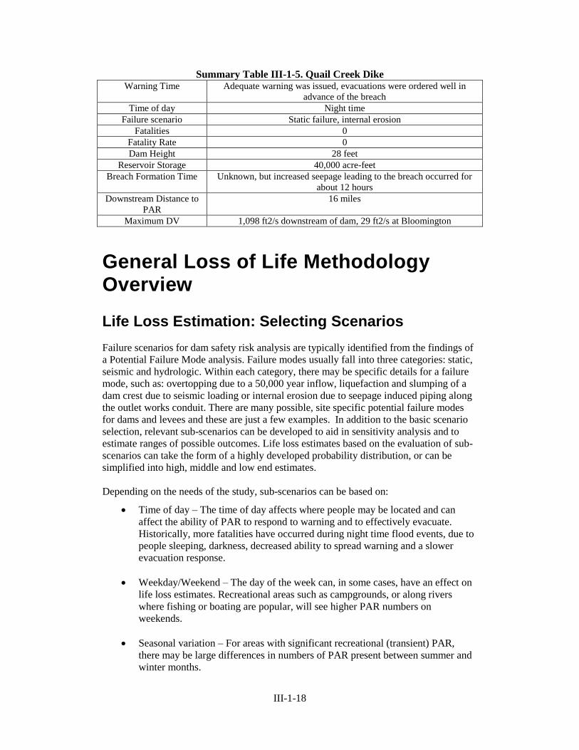
Summary Table III-1-5. Quail Creek Dike Warning Time Adequate warning was issued, evacuations were ordered well in

advance of the breach

Time of day Night time

Failure scenario Static failure, internal erosion

Fatalities 0

Fatality Rate 0

Dam Height 28 feet

Reservoir Storage 40,000 acre-feet

Breach Formation Time Unknown, but increased seepage leading to the breach occurred for

about 12 hours

Downstream Distance to

PAR

16 miles

Maximum DV 1,098 ft2/s downstream of dam, 29 ft2/s at Bloomington

General Loss of Life Methodology Overview

Life Loss Estimation: Selecting Scenarios

Failure scenarios for dam safety risk analysis are typically identified from the findings of

a Potential Failure Mode analysis. Failure modes usually fall into three categories: static,

seismic and hydrologic. Within each category, there may be specific details for a failure

mode, such as: overtopping due to a 50,000 year inflow, liquefaction and slumping of a

dam crest due to seismic loading or internal erosion due to seepage induced piping along

the outlet works conduit. There are many possible, site specific potential failure modes

for dams and levees and these are just a few examples. In addition to the basic scenario

selection, relevant sub-scenarios can be developed to aid in sensitivity analysis and to

estimate ranges of possible outcomes. Life loss estimates based on the evaluation of sub-

scenarios can take the form of a highly developed probability distribution, or can be

simplified into high, middle and low end estimates.

Depending on the needs of the study, sub-scenarios can be based on:

Time of day – The time of day affects where people may be located and can

affect the ability of PAR to respond to warning and to effectively evacuate.

Historically, more fatalities have occurred during night time flood events, due to

people sleeping, darkness, decreased ability to spread warning and a slower

evacuation response.

Weekday/Weekend – The day of the week can, in some cases, have an effect on

life loss estimates. Recreational areas such as campgrounds, or along rivers

where fishing or boating are popular, will see higher PAR numbers on

weekends.

Seasonal variation – For areas with significant recreational (transient) PAR,

there may be large differences in numbers of PAR present between summer and

winter months.

III-1-19

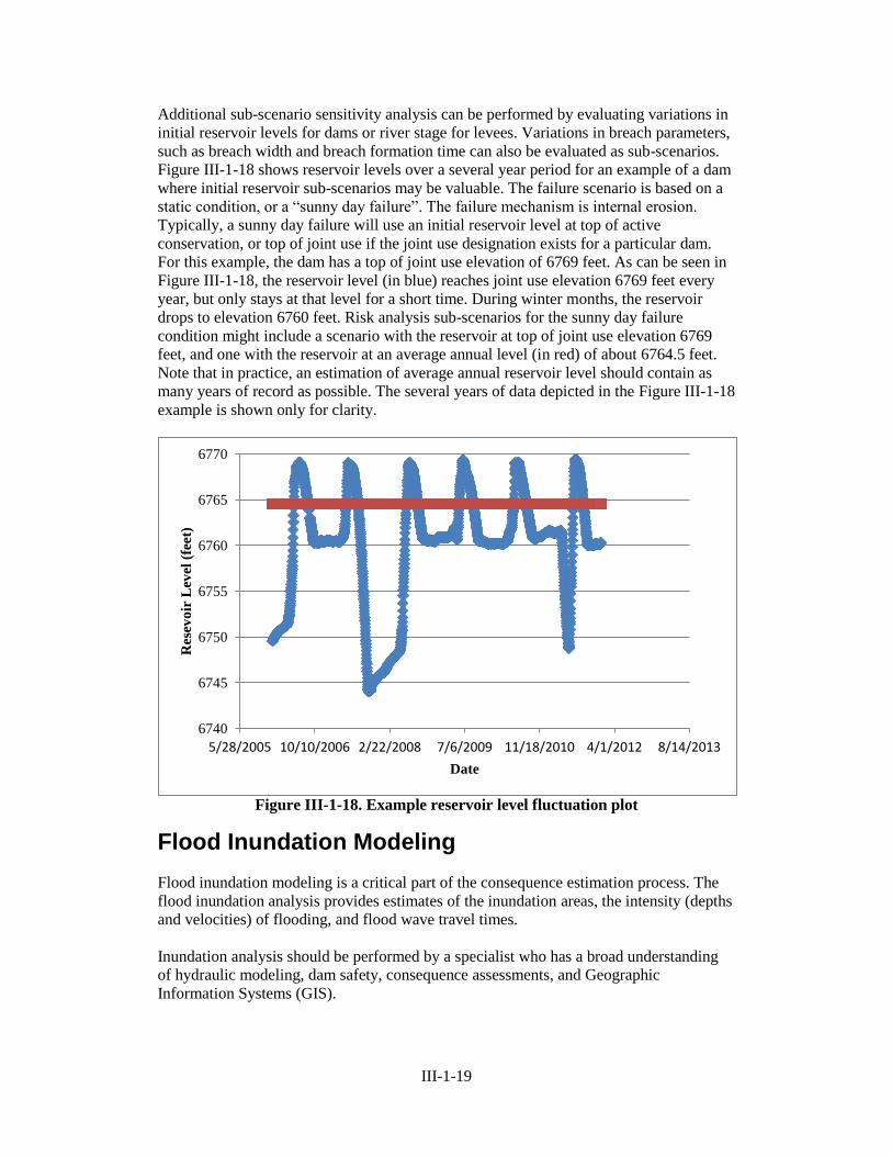
Additional sub-scenario sensitivity analysis can be performed by evaluating variations in

initial reservoir levels for dams or river stage for levees. Variations in breach parameters,

such as breach width and breach formation time can also be evaluated as sub-scenarios.

Figure III-1-18 shows reservoir levels over a several year period for an example of a dam

where initial reservoir sub-scenarios may be valuable. The failure scenario is based on a

static condition, or a “sunny day failure”. The failure mechanism is internal erosion.

Typically, a sunny day failure will use an initial reservoir level at top of active

conservation, or top of joint use if the joint use designation exists for a particular dam.

For this example, the dam has a top of joint use elevation of 6769 feet. As can be seen in

Figure III-1-18, the reservoir level (in blue) reaches joint use elevation 6769 feet every

year, but only stays at that level for a short time. During winter months, the reservoir

drops to elevation 6760 feet. Risk analysis sub-scenarios for the sunny day failure

condition might include a scenario with the reservoir at top of joint use elevation 6769

feet, and one with the reservoir at an average annual level (in red) of about 6764.5 feet.

Note that in practice, an estimation of average annual reservoir level should contain as

many years of record as possible. The several years of data depicted in the Figure III-1-18

example is shown only for clarity.

Figure III-1-18. Example reservoir level fluctuation plot

Flood Inundation Modeling

Flood inundation modeling is a critical part of the consequence estimation process. The

flood inundation analysis provides estimates of the inundation areas, the intensity (depths

and velocities) of flooding, and flood wave travel times.

Inundation analysis should be performed by a specialist who has a broad understanding

of hydraulic modeling, dam safety, consequence assessments, and Geographic

Information Systems (GIS).

6740

6745

6750

6755

6760

6765

6770

5/28/2005 10/10/2006 2/22/2008 7/6/2009 11/18/2010 4/1/2012 8/14/2013

Res

evo

ir L

evel

(fe

et)

Date

III-1-20

Often, when conducting a risk analysis, an inundation study may exist for a particular

dam or levee. An assessment of the existing study should be made to decide whether the

study results can adequately represent the scenarios to be evaluated during the risk

analysis. The following items should be considered when assessing the adequacy of an

existing inundation study:

Failure scenario - Is the failure scenario portrayed in the existing study

comparable to the desired scenarios for the new study? For example, a new

inundation study may be justified if the current study seeks to evaluate a sunny

day failure with normal reservoir levels, but the existing inundation study is

based on a Probable Maximum Flood (PMF) inflow where the inflow volume of

the flood increases the breach outflow by 100 percent over sunny day conditions.

Breach Parameters – Are the breach parameters for the existing study realistic?

Are they significantly different from the desired breach parameters of the failure

scenario to be evaluated by the risk analysis? An example might be a situation

that involves a large concrete gravity-arch dam. The existing inundation assumed

failure of the entire dam, all the way to the foundation. Recent finite element

structural analysis indicates that the dam, when subjected to the most severe of

loading conditions would only breach to the upper one-third of its height. In a

situation like this, a new inundation study may be justified.

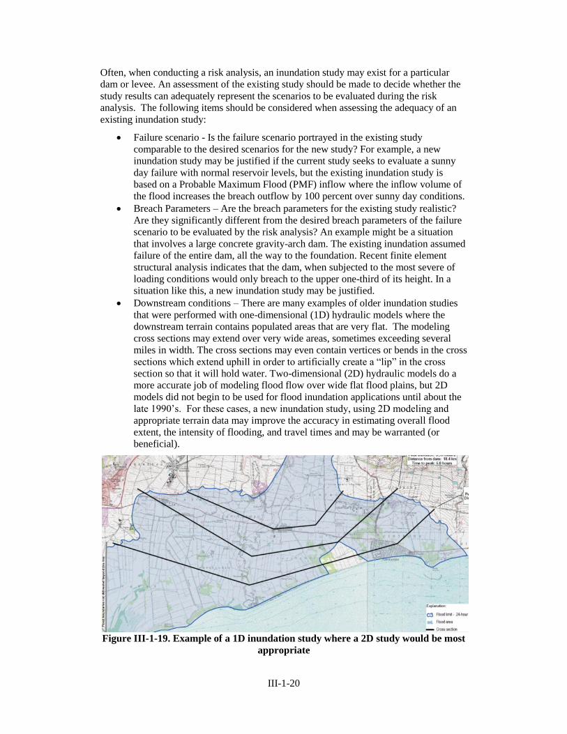
Downstream conditions – There are many examples of older inundation studies

that were performed with one-dimensional (1D) hydraulic models where the

downstream terrain contains populated areas that are very flat. The modeling

cross sections may extend over very wide areas, sometimes exceeding several

miles in width. The cross sections may even contain vertices or bends in the cross

sections which extend uphill in order to artificially create a “lip” in the cross

section so that it will hold water. Two-dimensional (2D) hydraulic models do a

more accurate job of modeling flood flow over wide flat flood plains, but 2D

models did not begin to be used for flood inundation applications until about the

late 1990’s. For these cases, a new inundation study, using 2D modeling and

appropriate terrain data may improve the accuracy in estimating overall flood

extent, the intensity of flooding, and travel times and may be warranted (or

beneficial).

Figure III-1-19. Example of a 1D inundation study where a 2D study would be most

appropriate

III-1-21

One Dimensional (1D) and Two Dimensional (2D) Hydraulic

Modeling for Flood Inundation Analysis Reclamation and USACE make use of different 1D and 2D hydraulic models for flood

inundation analysis. These models are described within the agency-specific sections of

this chapter. The following discussion contains general information regarding 1D and 2D

hydraulic modeling for flood inundation applications.

1D hydraulic models have traditionally been the standard for flood inundation

applications. Recently, 2D modeling has become more common practice when the

conditions of the study are such that 1D modeling cannot properly capture certain aspects

of the flood characteristics. Details of when 1D or 2D modeling should be applied to

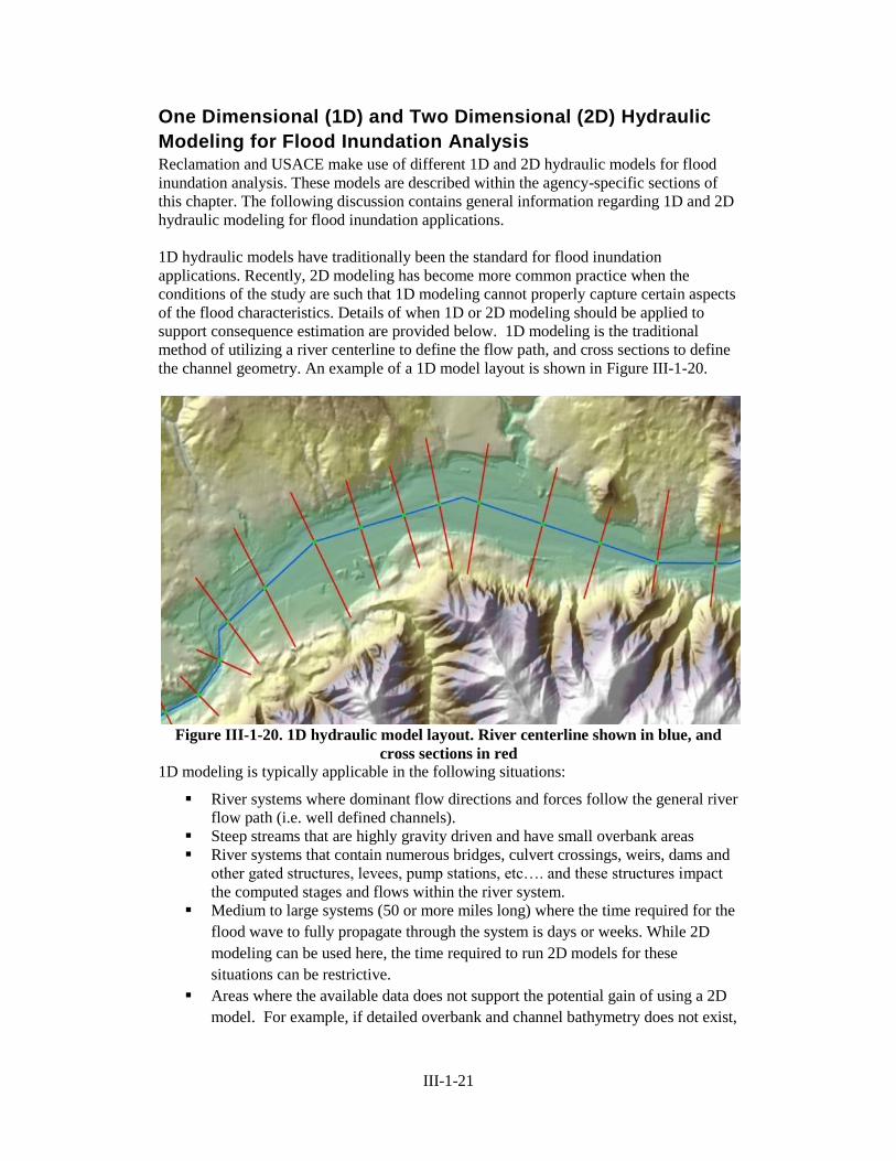
support consequence estimation are provided below. 1D modeling is the traditional

method of utilizing a river centerline to define the flow path, and cross sections to define

the channel geometry. An example of a 1D model layout is shown in Figure III-1-20.

Figure III-1-20. 1D hydraulic model layout. River centerline shown in blue, and

cross sections in red

1D modeling is typically applicable in the following situations:

River systems where dominant flow directions and forces follow the general river

flow path (i.e. well defined channels).

Steep streams that are highly gravity driven and have small overbank areas

River systems that contain numerous bridges, culvert crossings, weirs, dams and

other gated structures, levees, pump stations, etc…. and these structures impact

the computed stages and flows within the river system.

Medium to large systems (50 or more miles long) where the time required for the

flood wave to fully propagate through the system is days or weeks. While 2D

modeling can be used here, the time required to run 2D models for these

situations can be restrictive.

Areas where the available data does not support the potential gain of using a 2D

model. For example, if detailed overbank and channel bathymetry does not exist,

III-1-22

or the only data available includes detailed cross sections at representative

locations, many of the benefits of the 2D model will not be realized.

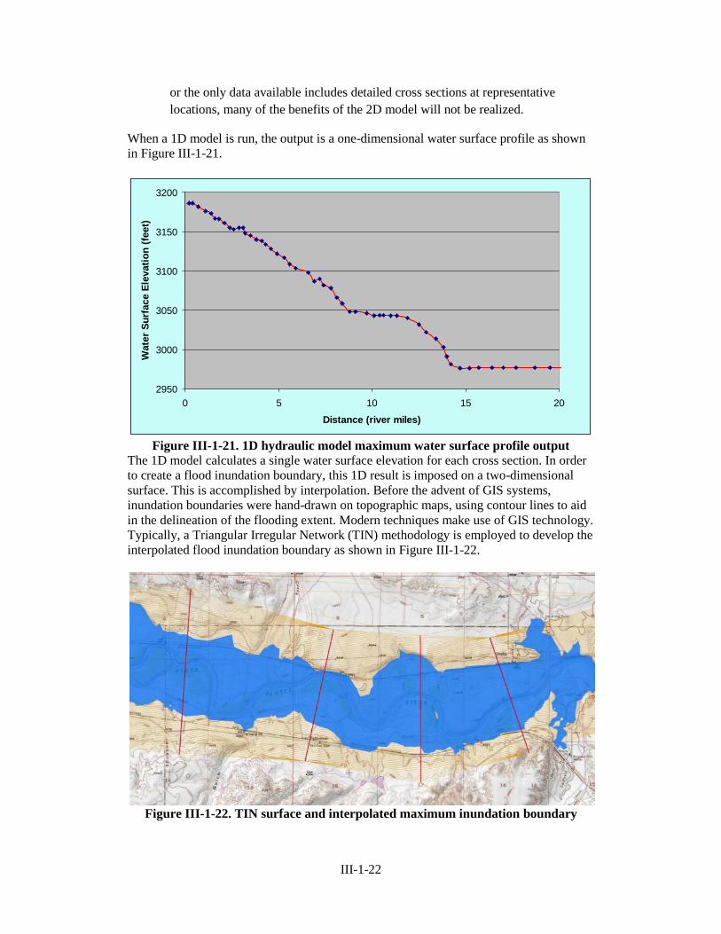
When a 1D model is run, the output is a one-dimensional water surface profile as shown

in Figure III-1-21.

Figure III-1-21. 1D hydraulic model maximum water surface profile output

The 1D model calculates a single water surface elevation for each cross section. In order

to create a flood inundation boundary, this 1D result is imposed on a two-dimensional

surface. This is accomplished by interpolation. Before the advent of GIS systems,

inundation boundaries were hand-drawn on topographic maps, using contour lines to aid

in the delineation of the flooding extent. Modern techniques make use of GIS technology.

Typically, a Triangular Irregular Network (TIN) methodology is employed to develop the

interpolated flood inundation boundary as shown in Figure III-1-22.

Figure III-1-22. TIN surface and interpolated maximum inundation boundary

2950

3000

3050

3100

3150

3200

0 5 10 15 20

Distance (river miles)

Wate

r S

urf

ace E

levati

on

(fe

et)

III-1-23

Advantages of 1D hydraulic models are:

Relatively short model run time – typically minutes to hours

Long reaches are more easily accommodated

Downstream hydraulic structures such as dams, culverts, bridges can be easily

included

1D model disadvantages are:

Does not provide as much detail or accuracy when considering velocities that

are not parallel to the stream centerline

Does not appropriately handle lateral spreading of flows in very flat flood plains

Inundation extents are interpolated

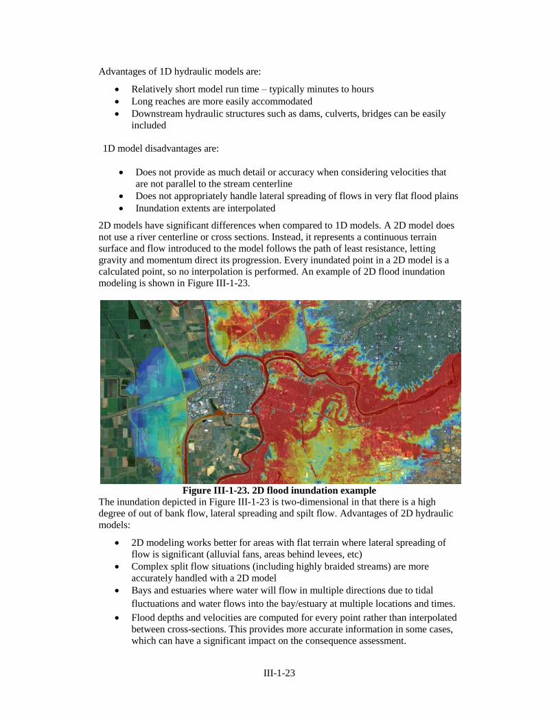
2D models have significant differences when compared to 1D models. A 2D model does

not use a river centerline or cross sections. Instead, it represents a continuous terrain

surface and flow introduced to the model follows the path of least resistance, letting

gravity and momentum direct its progression. Every inundated point in a 2D model is a

calculated point, so no interpolation is performed. An example of 2D flood inundation

modeling is shown in Figure III-1-23.

Figure III-1-23. 2D flood inundation example

The inundation depicted in Figure III-1-23 is two-dimensional in that there is a high

degree of out of bank flow, lateral spreading and spilt flow. Advantages of 2D hydraulic

models:

2D modeling works better for areas with flat terrain where lateral spreading of

flow is significant (alluvial fans, areas behind levees, etc)

Complex split flow situations (including highly braided streams) are more

accurately handled with a 2D model

Bays and estuaries where water will flow in multiple directions due to tidal

fluctuations and water flows into the bay/estuary at multiple locations and times.

Flood depths and velocities are computed for every point rather than interpolated

between cross-sections. This provides more accurate information in some cases,

which can have a significant impact on the consequence assessment.

III-1-24

2D model disadvantages are:

Relatively long model run times – multiple hours to days or even weeks to run a

simulation

Modeling extent and resolution (size of the model) are restricted by computer

hardware limitations – the larger the model, the longer it takes to run a

simulation, and it can be difficult to run long river reaches at a reasonable

terrain resolution

Model simulation time is also restricted by computer hardware limitations – this

is particularly true for hydrologic scenarios where spillway releases from a dam

occur for a long period of time prior to the initiation of a dam breach.

Note that highly detailed inundation modeling may not be justified when the estimation

of life loss consequences involves lightly populated areas.

Breach Parameters The selection of breach parameters for dams and levees can be an extremely important

consideration for consequence assessments. The breach parameters can affect the peak

breach discharge and the timing of the downstream flood arrival in a very significant

way.

1D numeric hydraulic models are typically utilized to develop breach outflow. There are

two breach mechanisms that are commonly used, piping and overtopping. The piping

breach formulation involves a hole in the embankment, which releases flow and

gradually becomes wider, eventually collapsing into a trapezoidal or rectangular shaped

breach. The overtopping breach formulation assumes that the breach is either trapezoidal

or rectangular, and that it forms from the crest of the structure downward, towards the

foundation.

The selection of breach parameters should be appropriate to the desired failure scenario.

For embankment dams, the width of a breach should account for the size of a reservoir

and the material properties. For example, the breach of a large volume reservoir may

mean a longer time for the reservoir to drain and this increases the chances for lateral

erosion. which will create a wider breach. At the same time, embankment material that is

erosion resistant may reduce the widening effect.

Historically, the failures of concrete dams have been observed to occur suddenly and

catastrophically. Examples of this are St. Francis Dam and Malpasset Dam.

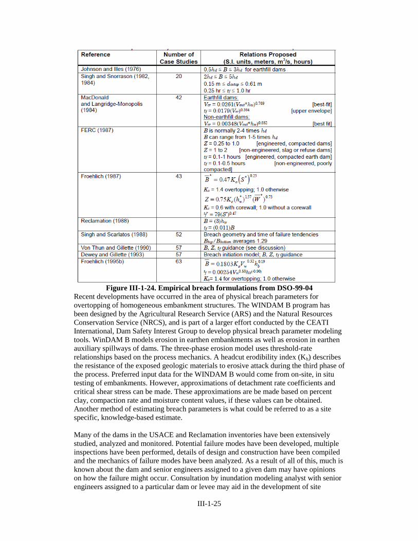
There are several approaches that can be used to estimate breach parameters. Empirical

formulations, based on dam failure case histories, have been widely applied to the

estimation of dam and levee breach analysis. The Reclamation report: Prediction of

Embankment Dam Breach Parameters, A Literature Review and Needs Assessment,

DSO-99-04, provides a summarization and analysis of commonly used empirical breach

parameter formulations. An excerpt of DSO-99-04 which briefly describes some

commonly used empirical breach formulations is shown in Figure III-124. It is important

to understand the range of case studies that the empirical equations are derived from

before applying them to a given dam.

III-1-25

Figure III-1-24. Empirical breach formulations from DSO-99-04

Recent developments have occurred in the area of physical breach parameters for

overtopping of homogeneous embankment structures. The WINDAM B program has

been designed by the Agricultural Research Service (ARS) and the Natural Resources

Conservation Service (NRCS), and is part of a larger effort conducted by the CEATI

International, Dam Safety Interest Group to develop physical breach parameter modeling

tools. WinDAM B models erosion in earthen embankments as well as erosion in earthen

auxiliary spillways of dams. The three-phase erosion model uses threshold-rate

relationships based on the process mechanics. A headcut erodibility index (Kh) describes

the resistance of the exposed geologic materials to erosive attack during the third phase of

the process. Preferred input data for the WINDAM B would come from on-site, in situ

testing of embankments. However, approximations of detachment rate coefficients and

critical shear stress can be made. These approximations are be made based on percent

clay, compaction rate and moisture content values, if these values can be obtained.

Another method of estimating breach parameters is what could be referred to as a site

specific, knowledge-based estimate.

Many of the dams in the USACE and Reclamation inventories have been extensively

studied, analyzed and monitored. Potential failure modes have been developed, multiple

inspections have been performed, details of design and construction have been compiled

and the mechanics of failure modes have been analyzed. As a result of all of this, much is

known about the dam and senior engineers assigned to a given dam may have opinions

on how the failure might occur. Consultation by inundation modeling analyst with senior

engineers assigned to a particular dam or levee may aid in the development of site

III-1-26

specific breach parameters, based on what is knowledge of the dam, its composition,

performance and its response in regards to potential failure modes. This approach may

include the analysis of empirical breach equations, but in many cases is just based on

informed opinions about the specific dam in question. There are a lot of uncertainties in

the prediction of breach parameters and this approach can be valuable in that it enables

collaboration and helps to build consensus between the inundation/consequences analyst

and those who will be using the study results for risk analysis.

Inundation Modeling Terrain Data Terrain data for inundation modeling is important. Current hydraulic models rely on GIS

for pre- and -post processing. Digital elevation models (DEM) have become the most

commonly used terrain data format. The DEM is a raster or grid based format, similar to

a matrix of equal sided cells containing a single elevation value. Some hydraulic models

make use of terrain data in a TIN surface format rather than a DEM format. Certain 2D

hydraulic models require the creation of what is called an unstructured mesh, which is a

network of various sized triangles or trapezoids. Surveyed cross section data are

sometimes used as well. In general though, there are several common types of digital

terrain data sources:

USGS DEMs – USGS produces DEMs which can be downloaded for free

from the National Elevation Dataset (NED) website, ned.usgs.gov NED

DEM data is usually available in 10 and 30-meter resolution. This is for the

most part, lower resolution terrain. However, the NED DEM data is widely

used and can be of adequate quality and resolution for modeling high

discharge dam breach flows downstream of large storage reservoirs.

IFSAR Terrain data – Interferometric Synthetic Aperture Radar (IFSAR)

data is radar-based terrain data which is collected from the wing of an

aircraft. IFSAR data is processed to remove vegetation, man made structures

and other features to produce a “bare earth surface”. The currently available

data is “medium quality resolution”, significantly better than the USGS NED

data. IFSAR data has 1-meter accuracy, both vertical and horizontal.

Intermap Technologies, www.intermap.com, has collected IFSAR terrain

data for the entire 48 U.S. mainland states. This data is readily available and

pricing of the data is very reasonable in comparison to higher resolution

options. IFSAR data can be a good option when USGS NED data does not

contain enough information to accurately portray downstream features. This

would be particularly true when modeling lower discharge dam breach or

levee breach flow and/or where flat terrain in downstream areas does not

contain enough detail in the USGS NED data to have confidence in the

modeling results.

Aerial Photogrammetry – Interpretation of aerial photography can produce

digital terrain data with a variety of accuracy that depends on photo scale

(flying height). This data can be very good quality, although it can be

expensive and time consuming to acquire. Photogrammetric data may have

cost advantages over LIDAR when detailed data is desired within a small

area.

LIDAR - Light detection and ranging data (LIDAR) is laser-based data that

is flown from an aircraft, much like the IFSAR data, but at a higher accuracy.

LIDAR data typically has a vertical accuracy of +/- 15 cm (about 6-inches).

III-1-27

The “bare earth surface” produced by LIDAR data is typically of very high

accuracy. LIDAR is expensive and time consuming to acquire, but when the

highest resolution data is needed, LIDAR may be the way to go. Note that

ground-based LIDAR systems also exist and may be of value to collect

detailed data within a small area of interest.

Using the power of a GIS, a wide variety of data formats can be utilized if available. For

example, vector contour line data can be converted to DEM format, point data can be

converted to TIN, TIN can be converted to DEM, etc. GIS technology allows the

integration of a wide variety of potential data sources.

Note that higher resolution data such as photogrammetric or LIDAR may have been

acquired by local entities who may be willing to share the data at low or no cost. There is

often value in contacting local county or city GIS offices to inquire about the existence of

such data.

In working with different terrain types, it is important to keep a perspective on terrain

accuracy versus terrain resolution. For example, changing the resolution (known as re-

sampling) of a USGS NED 10-meter DEM from 10-meters to 3-meters does not make the

data more accurate. However, re-sampling LIDAR data to a 10-meter resolution will

provide more accurate data than the 10-meter NED DEM, since the vertical accuracy of

the NED data is much lower than the LIDAR data. There are limits to this; re-sampling

LIDAR data to a 1,000 or even 100-meter resolution, for the purpose of creating faster

2D model run times loses all the benefits of vertical accuracy that were gained with the

LIDAR data.

The modeling of dam failure scenarios which include the operation and/or breaching of

downstream dams may require the development of downstream reservoir bathymetry in

order to properly represent the dam and reservoir in the model.

Inundation Modeling Outputs Inundation modeling outputs are used to develop a variety of information that is useful

for estimating life loss. A standard inundation modeling output is the maximum

inundation polygon. This is the flood boundary that is typically shown on an inundation

map. The maximum inundation polygon depicts the widest and most severe extent of

flooding that occurs in all of the downstream areas. In reality when upstream areas

become inundated, the downstream areas have not yet been flooded. When these

downstream areas reach maximum flooding, the upstream areas might start to dry out.

The maximum inundation polygon is useful for viewing the maximum flooding that may

occur at all flooded locations throughout the duration of the flooding event.

In additional to maximum inundation, typical inundation modeling output data includes

flood depths, velocities, water surface elevations, maximum discharge, arrival time of

leading edge and arrival time of maximum flooding.

1D models traditionally have presented output data at cross section locations. This data is

typically portrayed in a tabular format. On an inundation map, it is common to depict

cross sections, labeled by their location. A Table on the map will include output

information referenced to the cross sections.

2D models do not have cross sections and the presentation of 2D modeling results may

make use of a variety of formats. 2D inundation polygons can be color-coded according

III-1-28

to ranges of depth, velocity or DV. In addition to the maximum inundation polygon, it is

easy to display “snapshots in time” which depict the entire flood configuration at a

particular time of interest, for example - three hours after the initiation of the breach. The

leading edge of flooding is irregular and a poly line data set can be digitized in the GIS to

represent the front edge of the flood at various time steps. Maximum discharge and time

to maximum flooding information can be obtained by extracting hydrographs from the

2D model output data at areas of interest. Interpolated results from 1D modeling output

can be presented in a format similar to what is done with 2D modeling output. Care must

be taken though when presenting 1D results in this manner, not to misrepresent the

accuracy of the study in question.

Estimation of Downstream Population at Risk

Life loss estimates are based on some assumption of the number of people that are

present in the flood zone. There are different life loss estimation methods that take

various approaches to how they develop fatality estimates, but one thing these methods

all have in common is that they require an initial estimate of PAR. At a very basic level,

the development of a PAR estimate can be as simple as visiting a site below a dam or

levee and counting houses in the inundation zone. One of the online map services such as

Google Maps, Google Earth or MapQuest can also be used to count inundated houses.

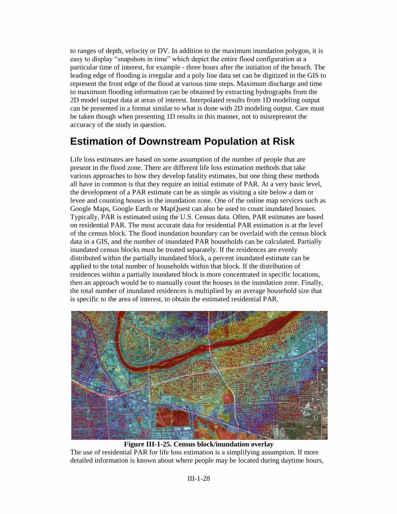
Typically, PAR is estimated using the U.S. Census data. Often, PAR estimates are based

on residential PAR. The most accurate data for residential PAR estimation is at the level

of the census block. The flood inundation boundary can be overlaid with the census block

data in a GIS, and the number of inundated PAR households can be calculated. Partially

inundated census blocks must be treated separately. If the residences are evenly

distributed within the partially inundated block, a percent inundated estimate can be

applied to the total number of households within that block. If the distribution of

residences within a partially inundated block is more concentrated in specific locations,

then an approach would be to manually count the houses in the inundation zone. Finally,

the total number of inundated residences is multiplied by an average household size that

is specific to the area of interest, to obtain the estimated residential PAR.

Figure III-1-25. Census block/inundation overlay

The use of residential PAR for life loss estimation is a simplifying assumption. If more

detailed information is known about where people may be located during daytime hours,

III-1-29

then this information can be used to develop daytime-specific life loss scenarios. Care

must be taken though, not to double count PAR when looking at non-residential PAR

distributions. A good example of this is a Reclamation Dam that has a mill operation

located immediately downstream. The mill has maybe 400 employees present during

daytime hours. The proximity of the dam to these employees puts them at the highest

level of risk in the event of dam failure. It is unknown however, where the residences of

these employees are located. Some may live in the flood zone at locations further

downstream, and because of this they may be double counted. In this case though, the

fatalities close to the dam can be assumed to be high and persons living downstream in

the floodplain are assumed to have much more time to evacuate, so that the issue of

potentially double counting is not considered to be introducing major errors. Double

counting of PAR when considering non-residential situations should be evaluated on a

case by case basis to avoid the possibility of overestimating fatalities.

Another type of PAR that is frequently estimated is recreational or transient PAR. This

would include persons occupying campgrounds, fishing, boating or hiking along a river,

etc. Recreational PAR estimates can be obtained through site visits and/or by consulting

with land use and recreation management groups who oversee these areas. In some cases,

visitation numbers data may be available, or in other cases, campground hosts or park

rangers may have a general idea of user numbers. Typically, recreational PAR will vary

by time of year and day of week, with great numbers in the summer months and on

weekends. Day use areas will of course have higher PAR during daytime hours, with low

or no PAR present during the evening.

Warning and Evacuation

In the most ideal situation, a dam breach in progress would be detected well in advance

of the beginning of catastrophic outflows, clear evacuation orders would issued to

downstream PAR without delay, and all of the PAR would move safely out of the flood

zone by the time flooding arrives in their area. Unfortunately, dam failure and flash flood

case histories have shown that things don’t always go that smoothly. The sequence of

events that takes place is often a mix of physical and social phenomena, sometimes

combined with a dose of luck or chance.

The issuance of warning and the decision of downstream PAR are critical factors that

impact the potential for life loss. Past dambreak flood instances show that, in general, the

number of fatalities decreases as the distance downstream increases, but increasing

distance by itself is not what decreases the life loss potential. Potential life loss decreases

when the travel time begins to exceed the amount of time required to warn and evacuate

the population at risk. A combination of breach development rate and flood wave

velocity determines the flood wave arrival time for a given distance. Then, the distance

to a safe haven, the escape route capacity, and various human perceptions and choices

determines who might be caught within inundation boundaries when the flood arrives.

Another attribute of increasing distance is the attenuation (reduction) in flow that occurs.

However, flow depths and velocities can increase downstream if the flood plain

transitions from a wider valley to a narrow canyon.

Warning time is broken into stages: detection of the threat, decision to issue warning,

notification of the downstream PAR, and warning dissemination. Detection of a

developing dam failure situation could be by automated instrumentation, by visual

III-1-30

inspection by project personnel or by someone passing by the area such as a hiker or

fisherman. After the unusual situation is noticed, some time is required before project

and emergency preparedness personnel assess the situation and decide that there is a

reasonable chance it will develop into a condition that cannot be controlled. Then, the

notification of those responsible for spreading the warning can take some time. The

actual warning to the population at risk can be transmitted many ways, each with its own

degree of effectiveness. The content and wording of the warning message is very

important when it comes to how quickly people will take the necessary precautions,

either giving people a strong perception of the danger or not. Warning can also spread by

word-of-mouth through friends, family, neighbors, and concerned citizens. People who

are at risk, but are not warned verbally, can still perceive danger by hearing an unusual

sound or seeing a rapidly rising flow.

Estimation of the warning and evacuation process may include consideration of the

following issues:

Failure of the dam or its impending failure may need to be verified before

warning is issued.

The decision to order evacuations must be made. Often the decision makers will

weigh the evidence at hand regarding the likelihood of catastrophic flooding vs.

perceived issues of public distrust when determining whether to issue a warning.

After a warning is issued, it will spread through the targeted community. The

speed at which is spreads is based on the types of warning systems/channels

employed by the agency issuing the warning. There is no silver bullet when it

comes to the best, most effective warning system. Research shows that using a

wide range of traditional and recent technology provides the most efficient

warning dissemination.

People may receive warning or an order to evacuate, but may delay taking a

protective action (e.g. evacuation) or may choose not to leave at all. The

timeliness of taking the recommended protective action is heavily influenced

based on the content of the warning message. Clear messages that contain

information about the threat, the source of the warning, the potential

consequences, specific instructions on when to leave and where to go are much

more likely to lead to a quick response than those lacking information.

Persons who do not attempt to evacuate or who attempt to evacuate at the last

minute can be placed in critical situations where a number of factors may

influence their survival. The flood depths, the intensity of flooding (often

quantified as a function of depth and velocity), the strength of a shelter, and a

person’s physical condition will influence the survival chances of PAR exposed

to flooding.

Some people may not evacuate. Reasons for this include: warnings may not be

taken seriously; elderly persons or disabled persons may have too much difficulty

attempting to evacuate; people may not evacuate for fear of looting; people may

not believe that the flood impacts will be severe enough to endanger them;

people delay evacuation to protect personal property such as pets or livestock.

Densely populated urbanized areas need more time to evacuate. These are special

situations where traffic congestion may play a role in the ability to evacuate.

Persons attempting to evacuate in advance of flooding may get stuck in traffic,

III-1-31

resulting in exposure to flooding. In many situations, evacuating to a large,

sturdy building, or staying in one’s home may be safer than attempting to leave

the area in a vehicle. Note that life loss simulation models such as LifeSim and

Life Safety Model use transportation network models and attempt to address

traffic congestion issues during flood events.

Case history data provides some examples of human behavior in relation to flood risk and

evacuation:

The failure of the Macchu II Dam in India in 1979 killed as many as 25,000

people. Once warned, some people didn’t leave because they lived above the

highest flood levels that had occurred during their lifetime.

Teton Dam failure in 1976 (11 fatalities) and Lawn Lake Dam failure in 1982 (3

fatalities) both contained fatality incidents where people who had safely

evacuated re-entered the flood zone to retrieve possessions, thinking that they

had more time before the arrival of flooding.

The eruption of the Nevado del Ruis volcano and the deadly lahar mudflow flood

at Armero, Columbia in 1986 killed about 22,000 people. Most residents of

Armero didn’t evacuate because the severity of risk was downplayed by local

officials.

St. Francis Dam failed in 1928, killing more than 400 people. Some who heard

the approaching flood waters could not conceive of a dam failure flood and

thought the sounds to be due to a windstorm.

Experience indicates that there is sometimes a reluctance to issue dam failure warnings.

The operating procedures or emergency actions plan that may be available for a dam or

levee should provide some guidance regarding when a warning would be issued. There is

no assurance, however, that a warning would be initiated as directed in a plan. A study

investigating loss of life from dam failure can be used to highlight weaknesses in the dam

failure warning process and provide some guidance on how improvements in the process

would reduce the loss of life. Sensitivity analysis should be used to provide information

on how significant warning issuance is to the uncertainty in a life-loss estimate.

For most breach mechanisms where the breach progression is observable prior to

catastrophic failure of the dam or levee, the time when a warning is issued should be

determined by first estimating the time when a major problem would be acknowledged

relative to the time of dam failure. The major problem acknowledgment time for these

failure modes is the time when a dam owner would determine that a failure is likely

imminent and they would decide that the dam breach warning and evacuation process

should be initiated by notifying the responsible authorities. The time lag between major

problem acknowledgement and when an evacuation order would pass from the dam

owner to the responsible emergency agency (EMA) and then from the EMA to the public

should be estimated based on available research, judgment of consequence specialists

familiar with that research, dam operations personnel and emergency management

personnel who have jurisdiction in the areas of each downstream community.

The amount of time it takes from when the evacuation warning is issued by the

responsible agency (warning issuance) until the population at risk receives that warning is

dependent on the number and type of warning systems or processes that are used to

disseminate that warning. A typical warning would be received by the population through

various means. For example, the first group of people would typically receive warning

through the primary warning process (e.g. Emergency Alert System), but then a

III-1-32

secondary warning process would begin that includes emergency responders and the

general population spreading that warning via word of mouth.

Intensity of Flooding and Fatality Rate

Fatality rates represent the percentage of people exposed to flooding (typically known as

threatened population) that lose their life. An important difference between RCEM and

the simulation models used by USACE and Reclamation is that RCEM defines fatality

rates as the percentage of pre-evacuation PAR that loses their life rather than a percentage

of exposed exposed to the flooding (those remaining after evacuation has taken place). In

either case, fatality rates are typically derived from empirical data.

The intensity of flooding can be correlated to the potential for fatalities. This intensity is

often quantified in terms of depth multiplied by velocity, or DV. Mapping of DV can be

produced from 1D or 2D modeling results and the DV maximum inundation boundary

can be overlaid with census data in a GIS to assess zones of various levels of destructive

intensity (also referred to as flood severity). Note that 2D hydraulic modeling can provide

greater accuracy when assessing lateral variation of DV. Flooding depths are an

important measure of flood intensity as well. Deeper water can make evacuation on foot

impossible, submerge roads, float cars and mobile homes, and make structures

uninhabitable. Fatality rates can be influenced by both flood depths and DV.

The potential for collapse of buildings within the flood zone can be some measure of the

potential for fatalities, assuming people are present when the flood arrives. Most

residential buildings would be vulnerable to major damage and/or collapse when flooding

DV exceeds the range of 7 to 15 m2/s.

Modeling assumptions that affect fatality rates can be adjusted when justified by

extenuating circumstances. If a particularly devastating earthquake is responsible for

dam failure, it is possible the earthquake has also devastated infrastructure and

communications in population centers in the vicinity. Every aspect of warning (i.e.

detection, decision, notification, and dissemination) may be affected, and evacuation

routes may be compromised. Emergency management personnel would be responding to

several situations and will not be able to devote their entire attention on a developing

situation at a dam. Using RCEM, it may be reasonable to increase the fatality rates for

this case. For the simulation-based approaches, these considerations would be handled

explicitly by adjusting the parameters in the warning and evacuation modeling.

Regardless of the life loss prediction method that is used, there is a great deal of

uncertainty in all aspects of the life loss estimate. Therefore, communicating risk to

decision-makers should be as a range, or better yet, as a graphical depiction of likelihood.

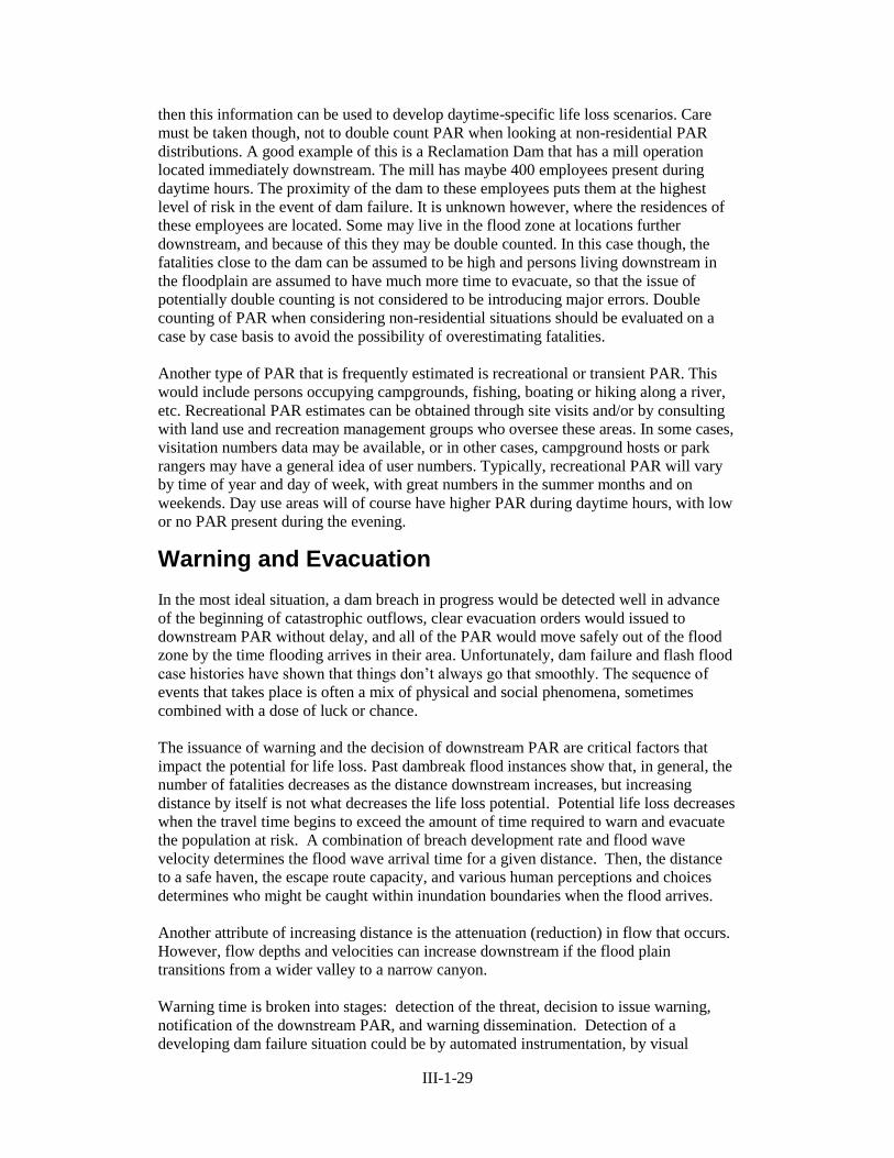
The general shape of likelihood distribution graphs can be envisioned by thinking

through many hypothetical scenarios. For example, many Reclamation dams have few

people living within the dam break flood inundation boundaries, and many failure

scenarios can be envisioned taking place very slowly with a long warning period. In

these situations, it would make sense that there would be a significant likelihood of zero

life loss. One could envision many dam break scenarios for the same dam and

population, starting at different times of the day, breaching with different rates, and given

various warning and evacuation scenarios. If many of these scenarios would end in life

loss, there might be a range between zero and some number where the estimate is likely

to fall. One could also envision some small chance that everything could go wrong, and

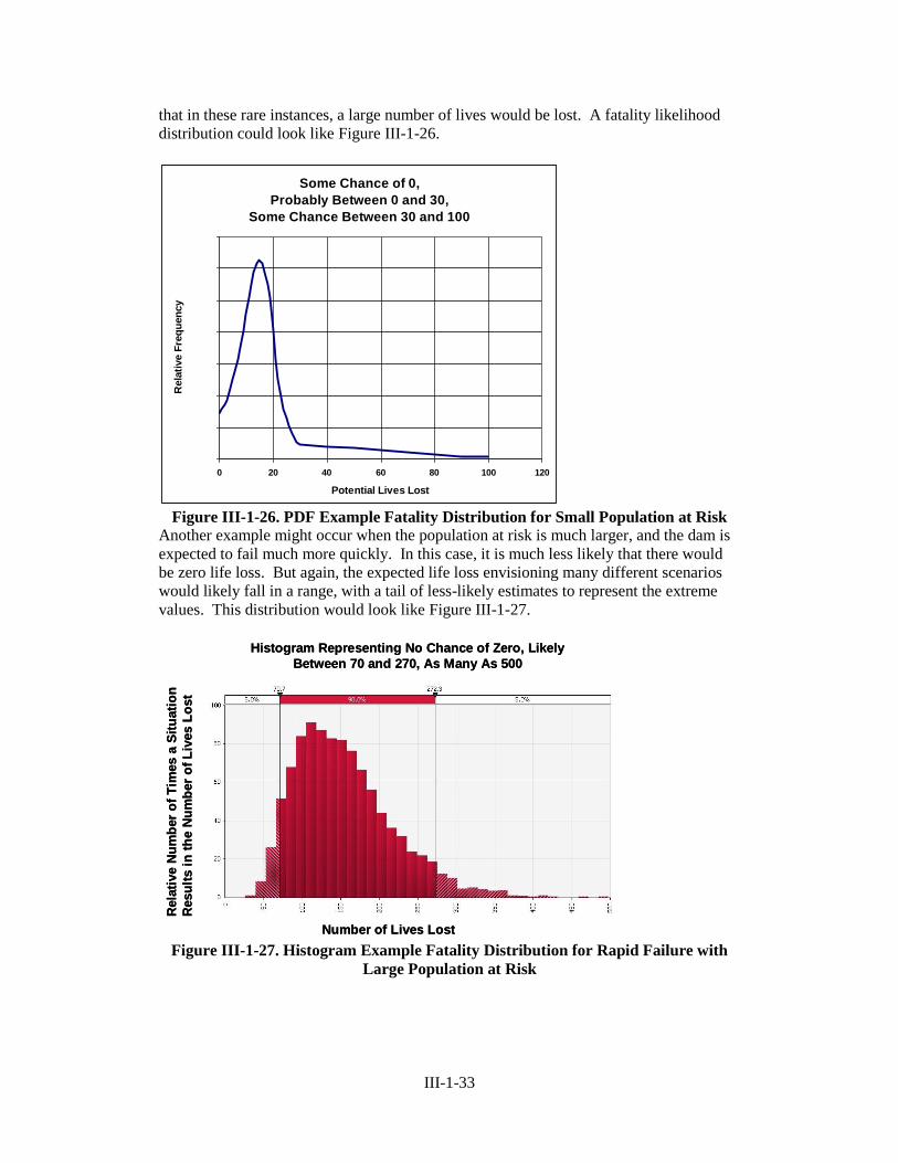
III-1-33

that in these rare instances, a large number of lives would be lost. A fatality likelihood

distribution could look like Figure III-1-26.

Figure III-1-26. PDF Example Fatality Distribution for Small Population at Risk

Another example might occur when the population at risk is much larger, and the dam is

expected to fail much more quickly. In this case, it is much less likely that there would

be zero life loss. But again, the expected life loss envisioning many different scenarios

would likely fall in a range, with a tail of less-likely estimates to represent the extreme

values. This distribution would look like Figure III-1-27.

Figure III-1-27. Histogram Example Fatality Distribution for Rapid Failure with

Large Population at Risk

Some Chance of 0,

Probably Between 0 and 30,

Some Chance Between 30 and 100

0

0.01

0.02

0.03

0.04

0.05

0.06

0.07

0 20 40 60 80 100 120

Potential Lives Lost

Rela

tive F

req

uen

cy x

Histogram Representing No Chance of Zero, Likely

Between 70 and 270, As Many As 500

Number of Lives Lost

Rela

tive N

um

ber

of

Tim

es a

Sit

uati

on

Resu

lts i

n t

he N

um

ber

of

Liv

es L

ost

Histogram Representing No Chance of Zero, Likely

Between 70 and 270, As Many As 500

Number of Lives Lost

Rela

tive N

um

ber

of

Tim

es a

Sit

uati

on

Resu

lts i

n t

he N

um

ber

of

Liv

es L

ost

III-1-34

Reclamation Consequence Estimating Methodology (RCEM)

Since September 1999, life loss from assumed failure of a Reclamation dam has been

estimated using the published document “A Procedure for Estimating Loss of Life

Caused by Dam Failure,” or report DSO-99-06. RCEM is very similar to the DSO-99-06

approach. DSO-99-06 provided suggested fatality rates to be applied to downstream

populations subjected to dam breach flows, considering the warning time, flood severity,

and flood severity understanding. RCEM involves consideration of these same elements

as well as other factors when selecting a fatality rate for a given exposed population, and

features a graphical presentation of fatality rates versus warning time and flood severity.

DSO-99-06 was based on the analysis of dam failures, flash floods and other floods

located primarily in the United States. Additional case histories were investigated for

RCEM and added to the database that forms the basis for the empirical approach. The

new database of flooding case histories has been expanded by more than 50 percent.

For the past 15 years, Reclamation has preferred an empirical approach to estimating life

loss; one based on interpretation of dam failure and flood case histories. RCEM

continues to rely on case history data to guide the selection of fatality rates. There is a

large uncertainty inherent in the estimation of life loss resulting from dam failure, in part

due to large possible variations in the development and progression of breach flows, as

well as numerous potential ways that the downstream public receives warning (if any)

and the manner in which they respond to warning. The study of flooding case histories

reinforces the finding that there are a wide range of possible outcomes from dam failure,

ranging from no fatalities to thousands of lives lost. The use of such empirical findings

and the resulting procedure based on these data are intended to reflect the variability

associated with life loss, as well as encourage the use of judgment in considering the

many variables associated with estimating life loss. Lessons learned from the case

histories show that a wide range of fatality rates are possible, and thus a range of life loss

should be portrayed rather than single point values.

Inundation Modeling at Reclamation

Reclamation’s inundation modeling work makes use of the Danish Hydraulic Institute

(DHI) MIKE models. MIKE11 is used for 1D modeling, and MIKE21 for 2D. These two

models can be linked or “coupled” using a utility known as MIKEFlood.

MIKE11 contains the National Weather Service DAMBRK breach formulation which

can be used for both piping and overtopping breach analysis. The MIKE11 model also

contains other structure routines for spillways, outlets, culverts, weirs and bridges. Multi-

dam breach analysis can be performed and logical operating conditions, useful for

modeling multi-dam scenarios, can be implemented. MIKE11 is linked to ArcGIS

through Model Interface One (MIO). MIO is a Reclamation developed interface to

ArcGIS for MIKE11 that allows pre- and post processing. MIKE11 river network

alignment and cross sections can be extracted from data in ArcGIS and directly imported

to a MIKE11 input file. 1D modeling results are then exported back into ArcGIS to create

an interpolated maximum inundation boundary using TIN methodology. MIO also allows

the interpolated TIN surface to be modified for various reasons such as addressing

III-1-35

inundation at tributaries and cutting off upstream TIN influences which may artificially

increase the extent o downstream inundation.

MIKE21 uses a structured mesh which allows direct import of DEM data from ArcGIS as

input terrain data. MIKE21 outputs are also easily exported back to ArcGIS for post-

modeling analysis. Hydraulic structures from MIKE11 can be linked to MIKE21 via

MIKEFlood. Terrain data can be modified to include features such as downstream river

levees or canal embankments using ArcGIS.

RCEM

The Relationship between Flood Severity and Fatality Rate The graphical approach to estimating the fatality rate utilized in RCEM is very similar to

the tabular approach described in DSO-99-06, which provides recommended ranges

based on case history data. However, the graphical approach involves greater

consideration of the case history database for making judgments about fatality rates.

Analysis of the case histories indicates that flood severity (a measure of the lethality of

the flood) and warning time are the factors that most influence the fatality rate for a

flood. The paragraphs that follow discuss the basis for establishing a relationship

between flood severity and fatality rate as the foundation for the graphical approach.

This relationship was established by studying the case history database and extracting

what was judged to be the best available information.

Flood severity, as developed within DSO-99-06, consists of low, medium, and high

severity flooding. RCEM goes beyond this category assignment and relies more on

assessing the flood severity as estimated by depth multiplied by velocity (DV). Flood

severity has a significant influence on fatality rate. Case history data indicate that the

highest observed fatality rates are associated with the highest estimated DV values.

When the flood severity is lower, there is a general trend of lower (or no) fatalities;

however, there is greater scatter in the fatality rates for lower flood severity values. In

developing RCEM, the numerical measure of flood severity, DV, was estimated for each

case history event using available documentation and engineering judgment. The

confidence level in the estimated DV varied depending on the amount and quality of the

available information.

The fatality rates are applied to the full population at risk, and do not explicitly consider

evacuation of downstream populations. The likely success of evacuations is something

that can be considered when selecting ranges for fatality rates using the RCEM

methodology. It is recognized that evacuation has a significant influence on the number

of fatalities from a flood. Obviously, for cases where the maximum number of people

was evacuated, the fatality rate with respect to the original PAR was lower – independent

of the DV value. However, the case history data do not provide a meaningful way to

extract PAR evacuation information such that a relationship involving evacuation as a

primary parameter can be established. Therefore, for the graphical approach, evacuation

is considered implicitly through the parameter of warning time – i.e., greater warning

time results in lower fatality rates because a greater portion of the PAR is able to

evacuate the flood area.

III-1-36

The amount of warning received by a PAR is typically part of the case history

documentation. For the same event, there may be several different population groups, and

each may have received a different amount of warning time. A review of the case history

data indicates that in most cases, the PAR received either little to no warning, or hours of

warning. The way that “some” warning was defined in DSO-99-06 is as a relatively

narrow window of time (between 15 and 60 minutes), and thus most cases have warning

times that tend to fall outside of these limits. For many of the older case histories (i.e.

prior to about the mid-1900s) communication networks and emergency management

systems were not in place to enable warning. In addition, there may have been a general

reluctance to issue a warning too soon, with operating personnel instead waiting until

failure was more certain or there may have been a lack of understanding that dam

overtopping could lead to dam failure. For these reasons, with older case histories,

receiving hours of warning was rare.

Given the above considerations, the basis or foundation for the graphical approach

involves establishing continuous relationships between flood severity and fatality rate for

different warning time scenarios. Because of the relative lack of case histories with

“some” warning time, only two warning time scenarios, little to no warning and adequate

warning, are used in RCEM. These terms are not tied to a specific amount of warning;

that is left to the judgment of those making the life loss estimates.

Graphical Approach – Suggested and Overall Limits Two charts were developed for selecting fatality rates using the graphical approach;

Fatality Rate vs. DV for Little or No Warning (Figure III-1-28), and Fatality Rate vs. DV

for Adequate Warning (Figure III-1-29).

Each chart includes dashed lines that represent “suggested” and “overall” limits for

fatality rates over the full range of DV values. The suggested limits were selected based

on the most representative case history data points for each warning time scenario. Cases

with questionable data were given less influence on the suggested range. The overall

limits are intended to represent the upper and lower bounds of fatality rates, between

which nearly all case history data falls.

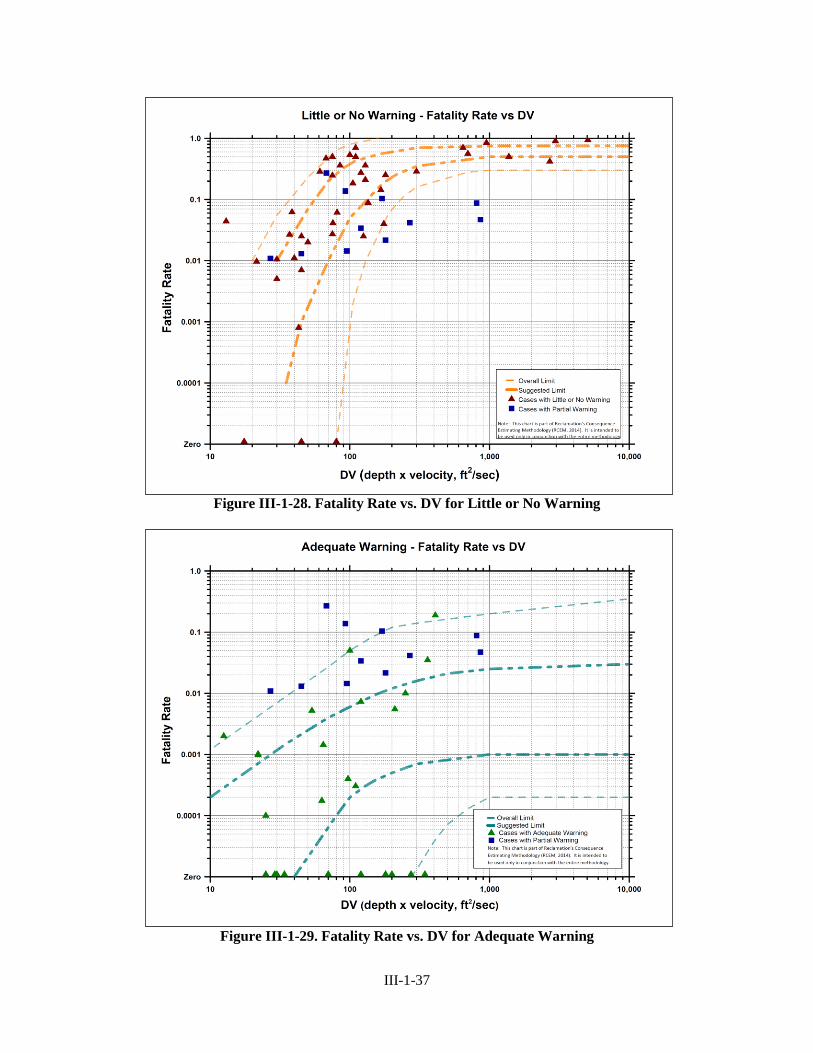
III-1-37

Figure III-1-28. Fatality Rate vs. DV for Little or No Warning

Figure III-1-29. Fatality Rate vs. DV for Adequate Warning

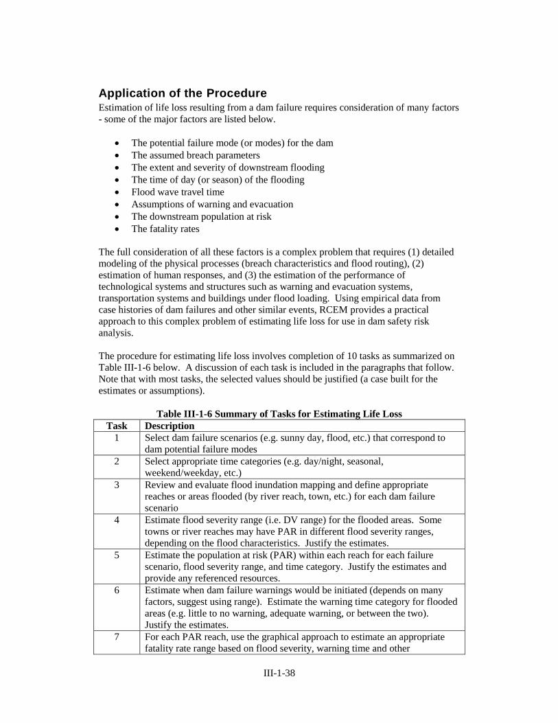
III-1-38

Application of the Procedure Estimation of life loss resulting from a dam failure requires consideration of many factors

- some of the major factors are listed below.

The potential failure mode (or modes) for the dam

The assumed breach parameters

The extent and severity of downstream flooding

The time of day (or season) of the flooding

Flood wave travel time

Assumptions of warning and evacuation

The downstream population at risk

The fatality rates

The full consideration of all these factors is a complex problem that requires (1) detailed

modeling of the physical processes (breach characteristics and flood routing), (2)

estimation of human responses, and (3) the estimation of the performance of

technological systems and structures such as warning and evacuation systems,

transportation systems and buildings under flood loading. Using empirical data from

case histories of dam failures and other similar events, RCEM provides a practical

approach to this complex problem of estimating life loss for use in dam safety risk

analysis.

The procedure for estimating life loss involves completion of 10 tasks as summarized on

Table III-1-6 below. A discussion of each task is included in the paragraphs that follow.

Note that with most tasks, the selected values should be justified (a case built for the

estimates or assumptions).

Table III-1-6 Summary of Tasks for Estimating Life Loss

Task Description

1 Select dam failure scenarios (e.g. sunny day, flood, etc.) that correspond to

dam potential failure modes

2 Select appropriate time categories (e.g. day/night, seasonal,

weekend/weekday, etc.)

3 Review and evaluate flood inundation mapping and define appropriate

reaches or areas flooded (by river reach, town, etc.) for each dam failure

scenario

4 Estimate flood severity range (i.e. DV range) for the flooded areas. Some

towns or river reaches may have PAR in different flood severity ranges,

depending on the flood characteristics. Justify the estimates.

5 Estimate the population at risk (PAR) within each reach for each failure

scenario, flood severity range, and time category. Justify the estimates and

provide any referenced resources.

6 Estimate when dam failure warnings would be initiated (depends on many

factors, suggest using range). Estimate the warning time category for flooded

areas (e.g. little to no warning, adequate warning, or between the two).

Justify the estimates.

7 For each PAR reach, use the graphical approach to estimate an appropriate

fatality rate range based on flood severity, warning time and other

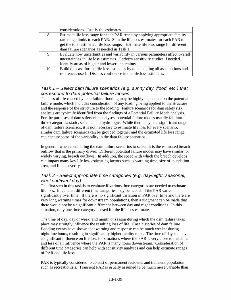
III-1-39

considerations. Justify the estimates.

8 Estimate life loss range for each PAR reach by applying appropriate fatality

rate range limits to each PAR. Sum the life loss estimates for each PAR to

get the total estimated life loss range. Estimate life loss range for different

dam failure scenarios as needed in Task 1.

9 Evaluate how uncertainties and variability in various parameters affect overall

uncertainties in life loss estimates. Perform sensitivity studies if needed.

Identify areas of higher and lower uncertainty.

10 Build the case for the life loss estimates by documenting all assumptions and

references used. Discuss confidence in the life loss estimates.

Task 1 – Select dam failure scenarios (e.g. sunny day, flood, etc.) that correspond to dam potential failure modes The loss of life caused by dam failure flooding may be highly dependent on the potential

failure mode, which includes consideration of any loading being applied to the structure

and the response of the structure to the loading. Failure scenarios for dam safety risk

analysis are typically identified from the findings of a Potential Failure Mode analysis.

For the purposes of dam safety risk analyses, potential failure modes usually fall into

three categories: static, seismic, and hydrologic. While there may be a significant range

of dam failure scenarios, it is not necessary to estimate life loss for every scenario;

similar dam failure scenarios can be grouped together and the estimated life loss range

can capture some of the variability in the dam failure scenarios.

In general, when considering the dam failure scenarios to select, it is the estimated breach

outflow that is the primary driver. Different potential failure modes may have similar, or

widely varying, breach outflows. In addition, the speed with which the breach develops

can impact many key life loss estimating factors such as warning time, size of inundation

area, and flood severity.

Task 2 - Select appropriate time categories (e.g. day/night, seasonal, weekend/weekday) The first step in this task is to evaluate if various time categories are needed to estimate

life loss. In general, different time categories may be needed if the PAR varies

significantly over time. If there is no significant variation in PAR over time and there are

very long warning times for downstream populations, then a judgment can be made that

there would not be a significant difference between day and night conditions. In this

situation, only one time category is used for the life loss estimate.

The time of day, day of week, and month or season during which the dam failure takes

place may strongly influence the resulting loss of life. Case histories of dam failure

flooding events have shown that warning and response can be much weaker during

nighttime hours, resulting in significantly higher fatality rates. The time of day can have

a significant influence on life loss for situations where the PAR is very close to the dam,

and less of an influence where the PAR is many hours downstream. Consideration of

different time categories can help with sensitivity analyses and can help estimate ranges

of PAR and life loss.

PAR is typically considered to consist of permanent residents and transient population

such as recreationists. Transient PAR is usually assumed to be much more variable than

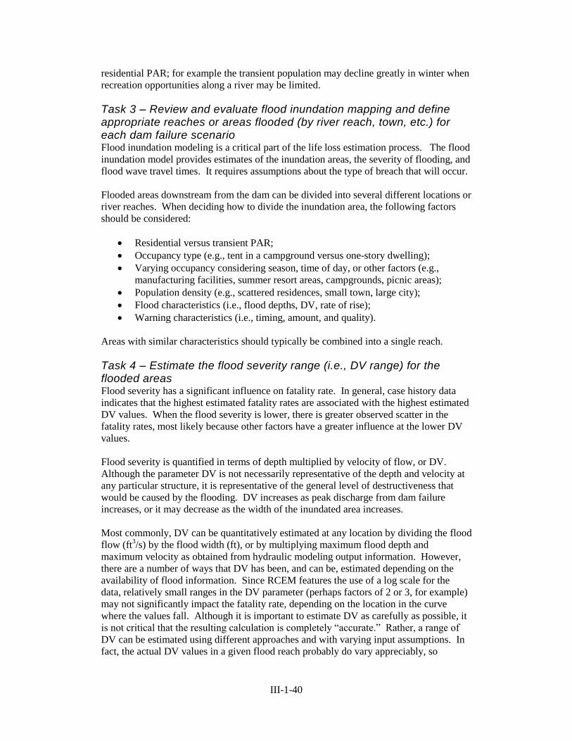
III-1-40

residential PAR; for example the transient population may decline greatly in winter when

recreation opportunities along a river may be limited.

Task 3 – Review and evaluate flood inundation mapping and define appropriate reaches or areas flooded (by river reach, town, etc.) for each dam failure scenario Flood inundation modeling is a critical part of the life loss estimation process. The flood

inundation model provides estimates of the inundation areas, the severity of flooding, and

flood wave travel times. It requires assumptions about the type of breach that will occur.

Flooded areas downstream from the dam can be divided into several different locations or

river reaches. When deciding how to divide the inundation area, the following factors

should be considered:

Residential versus transient PAR;

Occupancy type (e.g., tent in a campground versus one-story dwelling);

Varying occupancy considering season, time of day, or other factors (e.g.,

manufacturing facilities, summer resort areas, campgrounds, picnic areas);

Population density (e.g., scattered residences, small town, large city);

Flood characteristics (i.e., flood depths, DV, rate of rise);

Warning characteristics (i.e., timing, amount, and quality).

Areas with similar characteristics should typically be combined into a single reach.

Task 4 – Estimate the flood severity range (i.e., DV range) for the flooded areas Flood severity has a significant influence on fatality rate. In general, case history data

indicates that the highest estimated fatality rates are associated with the highest estimated

DV values. When the flood severity is lower, there is greater observed scatter in the

fatality rates, most likely because other factors have a greater influence at the lower DV

values.

Flood severity is quantified in terms of depth multiplied by velocity of flow, or DV.

Although the parameter DV is not necessarily representative of the depth and velocity at

any particular structure, it is representative of the general level of destructiveness that

would be caused by the flooding. DV increases as peak discharge from dam failure

increases, or it may decrease as the width of the inundated area increases.

Most commonly, DV can be quantitatively estimated at any location by dividing the flood

flow (ft3/s) by the flood width (ft), or by multiplying maximum flood depth and

maximum velocity as obtained from hydraulic modeling output information. However,

there are a number of ways that DV has been, and can be, estimated depending on the

availability of flood information. Since RCEM features the use of a log scale for the

data, relatively small ranges in the DV parameter (perhaps factors of 2 or 3, for example)

may not significantly impact the fatality rate, depending on the location in the curve

where the values fall. Although it is important to estimate DV as carefully as possible, it

is not critical that the resulting calculation is completely “accurate.” Rather, a range of

DV can be estimated using different approaches and with varying input assumptions. In

fact, the actual DV values in a given flood reach probably do vary appreciably, so

III-1-41

providing a range may be the best way to represent conditions. In most cases, this range

can be used with the graphs to come up with a reasonable fatality rate range.

Task 5 – Estimate the population at risk (PAR) within each reach for each failure scenario, flood severity range, and time category After DV values have been estimated in each flooded area, the PAR in each area is

estimated. For each combination of failure scenario, flood severity category, and time

category identified in Tasks 1, 2, and 4, the number of people at risk is estimated. PAR is

defined as the number of people occupying the dam failure flood plain prior to the

issuance of any warning or evacuation.

At a very basic level, the development of a PAR estimate can be as simple as visiting the

area downstream of a dam and counting houses in the inundation zone. PAR can also be

obtained using the inundation mapping data overlain with census data. A geographic

information system (GIS) is a powerful tool that can be used to simplify this process.

The most accurate data for residential PAR estimation is at the level of the census block.

When the flood inundation boundary can be overlain with the census block data in a GIS,

the number of inundated PAR households can be calculated. Partially inundated census

blocks must be treated separately. If the residences are evenly distributed within the

partially inundated block, a percent inundated estimate can be applied to the total number

of households within that block. If the distribution of residences within a partially

inundated block is more concentrated in specific locations, then the recommended

approach would be to manually count the houses (identified in aerial imagery) in the

inundation zone. Finally, the total number of inundated residences is multiplied by an

average household size that is specific to the area of interest (which can be obtained from

census data), to obtain the estimated residential PAR.

Task 6 – Estimate when dam failure warnings would be initiated and estimate the warning time categories for flooded areas (e.g., little to no warning, adequate warning, or between the two) Warnings refer to either specific notification of a developing or already in progress dam

failure issued by public officials, or an informal recognition and awareness of a

developing threat, perhaps passed by neighbors or simple observations of changing river

conditions.

In the most ideal situation, a dam breach in progress would be detected, well in advance

of the beginning of catastrophic outflows, and warnings and a strong evacuation order

would be issued to downstream PAR without delay, with all of the PAR moving safely

out of the flood zone by the time flooding arrives downstream. Dam failure and flash

flood case histories indicate the ideal situation does not always develop. The sequence of

events that takes place is often a mix of physical and social phenomena combined with

some element of chance or luck.

The recognition of a developing dam failure and the possible issuance of warning by

officials and subsequent PAR decisions regarding evacuation are critical factors that

impact the potential for life loss. However, an equally important consideration is flood

wave travel time, or how long before the dam failure flooding actually reaches a given

downstream reach.

III-1-42

Flooding case histories show that, in general, the number of fatalities decreases as the

distance downstream increases, but increasing distance by itself is not what decreases the

life loss potential. Potential life loss decreases when the travel time begins to exceed the

amount of time required to warn and evacuate the PAR. (Evacuation, or the lack thereof,

is accounted for in the fatality rates (using the pre-evacuation PAR) described in Task 7.)

Another result of increasing distance is the attenuation (reduction) in flow that occurs.

However, flow depths and velocities can increase downstream if the flood plain

transitions from a wider valley to a narrow canyon.

Assumptions regarding when formal or informal dam failure warnings for a particular

dam would be initiated can be based on an analysis of the monitoring/detection

(including the likelihood that anyone will observe a changing condition), decision

making, and notification systems or procedures for the dam. In many cases it may be

appropriate to estimate reasonable best case and worst case situations to bracket the time

when warnings would be initiated. This range of values can be used to estimate a range

of warning times.

The case history data generally indicates higher fatality rates for less warning time, and

vice versa. However, because of the large number of factors that influence each case,

similar fatality rates may result from different cases with different warning times. For the

purpose of estimating warning time using RCEM, two warning time categories are used:

Little to no warning (typically less than an hour)

Adequate warning (typically more than an hour, although there could be

situations with a dense population where hours of warning are not adequate)

After estimating the warning time range for each location, a judgment is made as to

which warning category would best represent that location. The distinction is important

because in Task 7, fatality rates are estimated using either a chart for “little to no

warning” or a chart for “adequate warning.” The exact determination of how many

minutes or hours of warning is not as important as the general category selected. As

discussed below under Task 7, the expected warning time (and quality) is a consideration

(along with other factors) when selecting the upper and lower limits of the recommended

and overall fatality rates.

Task 7 – For each PAR reach, use the graphical approach to estimate an appropriate fatality rate range based on flood severity, warning time and other considerations This task involves using all of the information available for a dam failure scenario to

estimate fatality rate ranges for each PAR area. For PAR areas that are assumed to

receive little or no warning, Figure III-128 is used, and for PAR areas that are assumed to

receive adequate warning, Figure III-1-29 is used. Each chart includes dashed lines that

represent “suggested” and “overall” limits for fatality rates over the full range of DV

values. The suggested limits provide a starting point for estimating the fatality rate range.

The selected fatality rate can be increased or decreased, based on all of the relevant

factors for each specific PAR area. The full limit ranges shown are not intended to be

used by estimators directly, but rather they are intended to help the estimator interpret the

approximate data trends from the case histories. For example, the range of overall limits

for little warning and a DV of 100 ft2/s covers about three orders of magnitude; however,

it is unlikely that the range of uncertainty in the fatality rate selected would span that full

III-1-43

range. Typically, the selected fatality rate range would be expected to span about one

order of magnitude. Judgment should be applied and a case should be built for selecting

a fatality rate range that is most appropriate for the situation being evaluated. The

application of judgment can include: comparison to relevant case histories, site specific

topographic/geographic/demographic considerations, evaluation of relative changes in

flow characteristics for a given reach when compared to an upstream reach, assumed

differences in warning time between subsequent reaches, and the potential for evacuation.

Judgment can also be applied between various potential failure modes in terms of

differing flow characteristics and anticipated warning times. It is acceptable to use a

fatality rate range with limits above or below the overall limits, as long as a case is built

for the estimated range, particularly that portion of the range that is beyond the limits of

the case history data.

Task 8 – Estimate life loss range for each PAR reach by applying appropriate fatality rate range limits to each PAR reach The range of estimated life loss for each specific PAR reach (corresponding to a location,

warning time, or flood severity) is determined by simply multiplying the appropriate

fatality rate range limits by each PAR estimate. For each dam failure scenario, the life

loss estimates from each PAR reach are summed to get the total estimated life loss range.

In addition to providing the range of total fatalities, a “best estimate” should be provided.

This best estimate may be the mean, a value derived by using suggested point values

within each reach, or a weighted average between seasonal or day/night combinations.

There is no “correct” way to determine this best estimate; it is up to the estimating team

to build a case for how to best represent the best estimate within the total estimated life

loss range.

Task 9 - Evaluate how uncertainties and variability in various parameters affect overall uncertainties in life loss estimates As evidenced by case histories, there can be a large range of fatality rates from dam

failure flooding. This is not surprising, considering the variability in PAR, severity of

flooding, and warning time. However, even within a given category of flood severity or

warning time there can still be a wide range of fatality rates. These differences may

result from having some of the PAR located near the river and some of the PAR located

farther away and thus less likely to feel the brunt of the flood flows. Similarly, not all

warnings are issued in the same manner, and different populations may respond quite

differently to warnings.

The graphical approach features “overall” limits to observed fatality rates; these are

essentially envelope curves that cover the majority of case history data points. Within the

overall limits are a set of “suggested” limits. Even these suggested limits typically show

significant differences between the upper and lower curve. Thus, case histories confirm

the uncertainty and variability inherent in the potential loss of life due to flooding. It is

important to recognize this uncertainty, and properly reflect it in final estimates by

portraying life loss as a range, often with an order of magnitude difference between upper

and lower bounds. In addition, the estimating team should consider what type of

probability distribution should be applied to any reported range. It is not unusual for a

life loss range to be reported as a uniform distribution, which implies that the life loss

really could fall anywhere within the range with equal likelihood. This would result in a

mean estimate in the middle of the range, reflecting a belief that the team finds no

III-1-44

compelling reason that the life loss would be expected to fall in either the high or low end

of the range.

Sometimes, the confidence in an estimate, as well as an understanding of uncertainty, can

be enhanced by a simple sensitivity analysis. Instead of assuming only a point estimate

for a particular parameter in a consequences analysis, a range in life loss can be

calculated by assuming different values for that variable. Approaching a life loss

evaluation in this manner will likely provide a better idea of the potential range of life

loss to be expected, as well as improve the confidence in the estimate.

Task 10 – Build the Case for the Life Loss Estimates

Building the case for the selected life loss estimates is a key requirement. The case for

the life loss estimates should address the key inputs that are included in the preparation of

the loss of life estimates, including: available inundation studies and the failure scenarios

and breach assumptions that they are based on the flow characteristics defined by the

inundation studies, the accuracy of census or other information used to estimate the

population at risk along the inundated area, the basis for assumptions of when warning

would be issued, any limitations on warning effectiveness and/or evacuation of the

population at risk, any unique site specific factors, and an overall rationale for the

selection of fatality rates. The case for the consequences should convince the reader and

ultimately the decision makers that the loss of life estimates are reasonable.

The case for the loss of life estimates should discuss the uncertainty inherent in the

estimates and the confidence that the risk analysis team has in the estimates. If sensitivity

studies indicate only small differences in the life loss estimates, confidence will be higher

in the estimates. Even if the loss of life estimates are sensitive to the assumptions, if the

overall dam safety findings are not changed based on the sensitivity studies, the overall

confidence in the findings may remain moderate to high. For example, although the life

loss estimates may vary by a factor or 2 or 3 depending on assumptions (indicating a

lower confidence in the estimated life loss), the total annualized life loss estimate may

still remain in the area indicating decreasing justification to take action.

Summary The estimation of life loss that might occur as a result of dam failure is a difficult task,

involving considerable uncertainty. Since the 1990s when Reclamation began utilizing

quantitative risk analysis as a tool to evaluate dam safety, life loss estimation has been

based on an empirical approach that utilized data from past flooding events. These data

illustrate the wide range of possible fatality rates that can occur during flooding events,

and provide valuable data and insights that can be applied in estimating potential life loss

from future dam failures. RCEM continues to be based on case histories, but has been

enhanced through the addition of many more historic flooding cases, as well as plotting

the data points in a way that illustrates the range of fatality rates observed in the case

history database. Engineering judgment and careful consideration of site-specific

conditions and potential failure modes are stressed as key requirements for application of

RCEM.

Example Application of RCEM The RCEM Examples of Use document includes four examples of application of the

methodology.

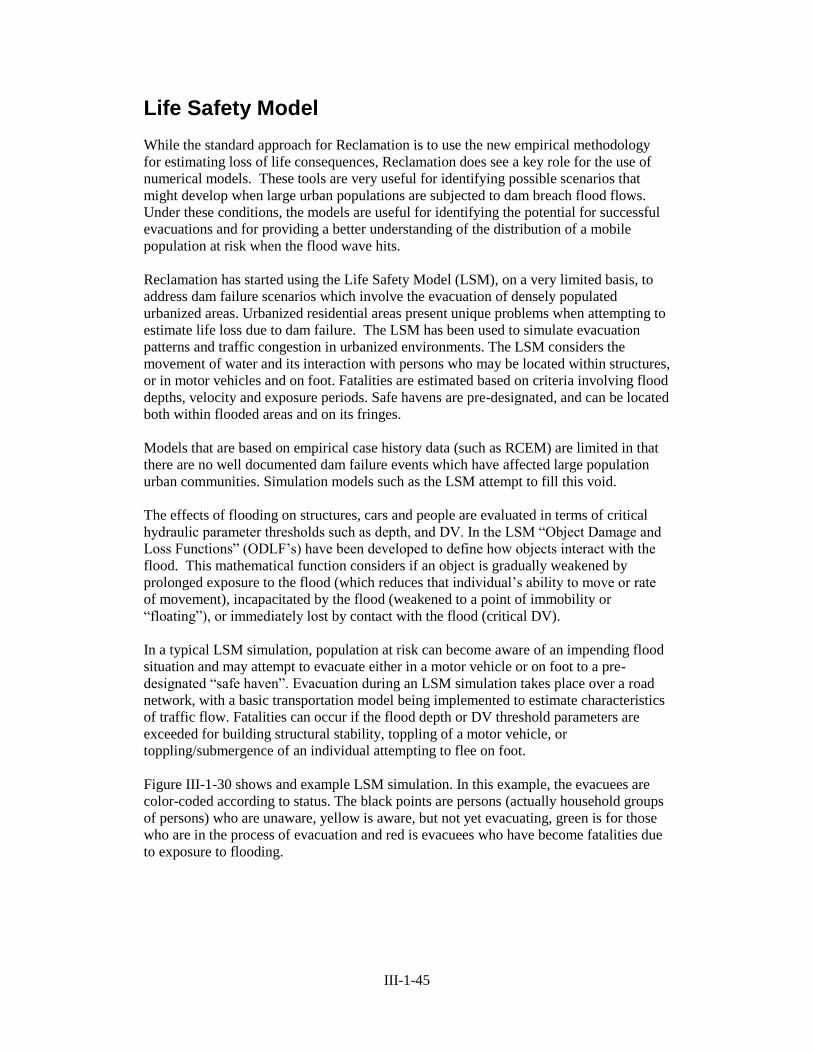
III-1-45

Life Safety Model

While the standard approach for Reclamation is to use the new empirical methodology

for estimating loss of life consequences, Reclamation does see a key role for the use of

numerical models. These tools are very useful for identifying possible scenarios that

might develop when large urban populations are subjected to dam breach flood flows.

Under these conditions, the models are useful for identifying the potential for successful

evacuations and for providing a better understanding of the distribution of a mobile

population at risk when the flood wave hits.

Reclamation has started using the Life Safety Model (LSM), on a very limited basis, to

address dam failure scenarios which involve the evacuation of densely populated

urbanized areas. Urbanized residential areas present unique problems when attempting to

estimate life loss due to dam failure. The LSM has been used to simulate evacuation

patterns and traffic congestion in urbanized environments. The LSM considers the

movement of water and its interaction with persons who may be located within structures,

or in motor vehicles and on foot. Fatalities are estimated based on criteria involving flood

depths, velocity and exposure periods. Safe havens are pre-designated, and can be located

both within flooded areas and on its fringes.

Models that are based on empirical case history data (such as RCEM) are limited in that

there are no well documented dam failure events which have affected large population

urban communities. Simulation models such as the LSM attempt to fill this void.

The effects of flooding on structures, cars and people are evaluated in terms of critical

hydraulic parameter thresholds such as depth, and DV. In the LSM “Object Damage and

Loss Functions” (ODLF’s) have been developed to define how objects interact with the

flood. This mathematical function considers if an object is gradually weakened by

prolonged exposure to the flood (which reduces that individual’s ability to move or rate

of movement), incapacitated by the flood (weakened to a point of immobility or

“floating”), or immediately lost by contact with the flood (critical DV).

In a typical LSM simulation, population at risk can become aware of an impending flood

situation and may attempt to evacuate either in a motor vehicle or on foot to a pre-

designated “safe haven”. Evacuation during an LSM simulation takes place over a road

network, with a basic transportation model being implemented to estimate characteristics

of traffic flow. Fatalities can occur if the flood depth or DV threshold parameters are

exceeded for building structural stability, toppling of a motor vehicle, or

toppling/submergence of an individual attempting to flee on foot.

Figure III-1-30 shows and example LSM simulation. In this example, the evacuees are

color-coded according to status. The black points are persons (actually household groups

of persons) who are unaware, yellow is aware, but not yet evacuating, green is for those

who are in the process of evacuation and red is evacuees who have become fatalities due

to exposure to flooding.

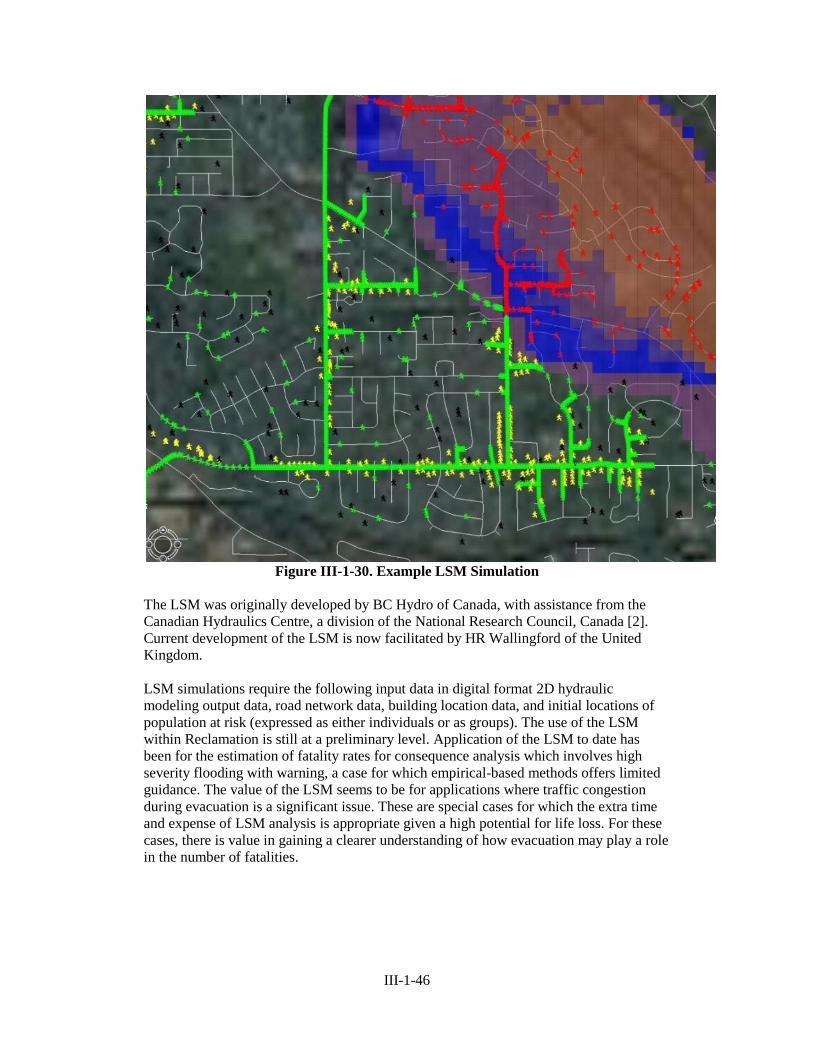
III-1-46

Figure III-1-30. Example LSM Simulation

The LSM was originally developed by BC Hydro of Canada, with assistance from the

Canadian Hydraulics Centre, a division of the National Research Council, Canada [2].

Current development of the LSM is now facilitated by HR Wallingford of the United

Kingdom.

LSM simulations require the following input data in digital format 2D hydraulic

modeling output data, road network data, building location data, and initial locations of

population at risk (expressed as either individuals or as groups). The use of the LSM

within Reclamation is still at a preliminary level. Application of the LSM to date has

been for the estimation of fatality rates for consequence analysis which involves high

severity flooding with warning, a case for which empirical-based methods offers limited

guidance. The value of the LSM seems to be for applications where traffic congestion

during evacuation is a significant issue. These are special cases for which the extra time

and expense of LSM analysis is appropriate given a high potential for life loss. For these

cases, there is value in gaining a clearer understanding of how evacuation may play a role

in the number of fatalities.

III-1-47

USACE Life Loss Estimation Methodology

Historically, development of life loss estimates for dam or levee failure scenarios has

been has not been common within USACE. Traditional dam safety management

practices only considered consequence estimates when making project specific

modification decisions, and those were usually limited to property damages. Detailed life

loss estimates were seldom required to support these decisions since a dam safety

modification could be justified simply by demonstrating the potential for one or more

fatalities. The priority and relative magnitude of dam safety issues under past USACE

practices was primarily focused on performance and adherence to design standards and

did not explicitly consider the potential consequences of failure. As a result, dam failure

consequence estimates for most dams (and levees) within the portfolio do not exist, are

outdated, or lack sufficient detail to adequately inform the USACE portfolio management

activities.

USACE promotes a scalable, decision-driven process for estimating consequences due to

dam or levee breach. That process implies that the level of detail and accuracy for a given

analysis must be appropriate to support the decision being made within a reasonable level

of confidence. For example, a screening level assessment could be used to support an

initial ranking for a portfolio of dams or levees via the USACE Dam or Levee Safety

Action Classification. This classification level could then be used to set priorities for

more detailed studies. This initial screening level assessment should require significantly

less effort and rigor than that for a detailed assessment used to determine what risk

reduction actions are needed to satisfy tolerable risk guidelines. The relative accuracy

required to get a “right” answer must not be taken out of the context of the decision to be

made. Too much effort can divert limited resources away from other critical dam or

levee safety needs just as too little effort potentially leads to poor decisions. The decision

driven nature of this risk process requires methods that can be easily scaled to the

appropriate level of effort needed. The life loss estimations tools used by USACE,

described below, fit the requirements of this scalable, decision-driven approach.

Since most decisions being made within the Dam Safety and CIPR Programs are initially

life safety related, the focus of this paper is on the methodology applied by USACE for

estimating population at risk (PAR) and loss of life.

Limitations of empirical approaches such as RCEM, DSO-99-06 and others that preceded

it are widely recognized and have resulted in the development of simulation-based

approaches to estimating loss of life. USACE, along with Reclamation and other

agencies, funded researchers at Utah State University to develop one such simulation

methodology known as LifeSim in the early 2000s. USACE has continued development

of this methodology and GIS based tools that can be used to apply the methodology for

dam or levee safety consequence assessments.

It was recognized early on that application of LifeSim can be very resource intensive.

Therefore, in order to satisfy the scalable, decision-driven approach described above, a

simplified version of LifeSim was developed and included in the Hydrologic Engineering

Center’s Flood Impact Analysis program (HEC-FIA). The LifeSim and simplified

LifeSim (HEC-FIA) procedures described herein are based on the foundation of

III-1-48

knowledge gained from an in-depth analysis of case histories conducted by D.M.

McClelland and D.S. Bowles.

Requirements for a typical application of LifeSim or HEC-FIA can be met from readily

available data including Census, FEMA’s HAZUS-MH, USGS Seamless and output from

a dam or levee breach inundation model, such as HEC-RAS, FLO-2D or any other

hydraulic model that generates results suitable for GIS processing.

As defined within the LifeSim framework, estimation of the magnitude of life loss

resulting from a dam or levee failure, whether due to a major natural event (such as a

flood or an earthquake), a design or construction defect, or a successful adversarial

attack, requires consideration of the following three groups of factors:

The flood event, including specific characteristics of the initiating event (i.e. for

flooding cause by dam or levee breach the following factors are important: the

breach location, geometry and rate of breach development, the water level behind

the dam or levee, the time of day, detection time of the breach-event relative to

breach initiation, and the extent, velocity, depth and arrival times throughout the

downstream inundation area.

The number and location of people exposed to the flood event, including the

initial spatial distribution of people throughout the inundation area, the

effectiveness of warnings, the response of people to warnings, the opportunity for

and effectiveness of evacuation, and the degree of shelter provided by the setting

where people are located (structure, vehicle, on foot, etc.) at the time of arrival of

the flood water.

The loss of life amongst the threatened population who remain in the

inundation area at the time of arrival of the flood water. Loss of life estimates at a

specific location take into consideration the physical character of the flood event

and the degree of shelter provided by the setting where people are located at the

time of arrival and after the flood wave has passed for those who survive it.

Clearly, the full consideration of all these factors is a very complex problem that requires

detailed modeling of the physical processes (breach characteristics and flood routing),

human responses, and the performance of technological systems (such as warning and

evacuation systems, transportation systems and buildings under flood loading).

USACE Inundation Modeling

USACE studies typically use the Hydrologic Engineering Centers River Analysis System

(HEC-RAS) to model dam and levee breach scenarios. HEC-RAS is a software tool that

performs one or two-dimensional steady and unsteady flow river hydraulics calculations,

sediment transport-mobile bed modeling, and water temperature analysis. HEC-RASis

endorsed by the USACE Hydrology, Hydraulics, and Coastal Community of Practice

(HH&C CoP), receive continued support within the agency, and is freely available for

downloading from the HEC website (www.hec.usace.army.mil). The link between HEC-

RAS or similar hydraulic tools and GIS facilitates the use of readily available and

existing data sets, efficient model development, and processing of results. New data and

information can be readily incorporated into existing models when improved accuracy is

needed. Once a current georeferenced HEC-RAS model is available for a dam, the

models can be updated as necessary when new information is available.

III-1-49

HEC-FIA (Simplified LifeSim)

The Simplified LifeSim methodology is applied within the HEC-FIA software program.

The applicability depends on the goals of the assessment as well as the characteristics of

the study area. The main differences between the Simplified LifeSim methodology

applied within HEC-FIA and the LifeSim methodology are as follows:

Evacuation Simulation - Simplified LifeSim uses a basic evacuation model where the

user either provides the amount of time required for inhabitants of each structure to

evacuate to safety or provides a hazard boundary in the form of a polygon shapefile. If a

hazard boundary is provided, HEC-FIA determines the shortest straight-line distance

from a structure to the hazard boundary and applies a nominal evacuation speed along

that line to estimate the amount of time required to evacuate. The effect of traffic jam

potential must be accounted for implicitly by the choice of the nominal evacuation speed.

If the loss of life for a study is highly dependent on evacuation efficiency, including the

effects of traffic congestion, application of the full version of LifeSim should be

considered as it contains a more detailed evacuation model.

Arrival Times - In Simplified LifeSim, flood arrival time at a structure is computed by

interpolating cross-section hydrograph output from a one-dimensional hydraulic model or

from a grid that contains arrival time values. The full version of LifeSim computes flood

wave arrival time by accessing a time-series of depth and velocity grids for the entire

flood event throughout the inundated area. Both models can utilize output from a two-

dimensional model.

HEC-FIA Inputs A technical description of the process and computations contained in HEC-FIA to

estimate life loss following the Simplified LifeSim methodology is provided later in this

paper. For instructions on using HEC-FIA, download the HEC-FIA User’s Manual from

www.hec.usace.army.mil. Inputs required by HEC-FIA to compute life loss and direct

property damage are described below:

Digital Elevation Grid: A digital elevation grid is required to compute consequences in

HEC-FIA. The digital elevation model is used to assign elevations to structures as well as

the elevation of the safe location in the evacuation effectiveness computation. The digital

elevation model used in HEC-FIA should be the same as the one used to develop the

hydraulic model of the dam break.

Structure Inventory with Population: All life loss estimates in HEC-FIA are done on

an individual structure basis. Therefore, an inventory that represents all the structures

within the flooded area is required. Each structure must have a ground elevation and

population assigned to it at a minimum, but the height of the structure is also important

(1-story, 2-story, etc).

If a detailed structure inventory does not exist for the study area, capabilities available in

HEC-FIA allow the user to generate a structure inventory for an area using an existing

parcel database (shapefile) or the database that comes with the FEMA HAZUS-MH tool.

When a structure inventory is generated using the HAZUS data, it should be checked

against aerial imagery to insure that it is representative of the study area.

III-1-50

The number of people in a structure often varies between day, night, weekday, and

weekends in residential, commercial and industrial areas. Population in a structure or area

can also vary significantly on a seasonal basis for campgrounds and other types of

recreational facilities, or areas of high tourism. Therefore, it is desirable to consider a

range of different exposure cases to capture the temporal variations in the numbers of

people in a structure. The number of people estimated in each structure should apply to

the time that an official public warning to evacuate would be issued for a dam failure for

each failure event that is considered. It is important to consider the fact that certain flood-

initiated failure events occur only during a specific season of the year and that the range

of reservoir pool elevations is commonly highly correlated with season of the year.

Capabilities available in HEC-FIA allow the user to generate day and night populations

for an existing structure inventory using the most recent census data (HAZUS). Day and

night populations estimated by HEC-FIA take into account the shift of population in an

area due to working in or out of the area during the day and returning home during the

evening and other similar considerations. Additionally this methodology splits the

population into the category of being over or under the age of 65 since those individuals

over 65 have been shown to be at higher risk of life loss in flood events. In this

methodology the population distribution between day and night on weekends is being

treated to be the same as during the weekdays.

Seasonal considerations and development that has occurred since the most recent census

are not included in the default population distribution provided by HEC-FIA. For areas

with high seasonal variability, the population in HEC-FIA will be based on the

“permanent” population of the area that is representative of the number of people that

identified that location as their primary residence in the most recent census. The user has

the ability to define population increases and decreases at the impact area level, which

could represent neighborhoods, towns, or counties. Another way to approximate the

effects of seasonal variations in population or population changes is to take the final life

loss results computed by HEC-FIA and factor them up or down as appropriate.

Transient population (i.e. campground and other recreation) should be considered

explicitly and included as appropriate when developing estimates for PAR. In HEC-FIA,

structures should be added to the inventory to represent tents or campers in a

campground. They will not be added automatically from the HAZUS inventory.

Population should also be added to those structures.

Recreational PAR for a campground should be based on visitation information for

impacted downstream recreation areas (not the ones around the lake which are considered

in project benefits foregone) and the duration of average visit when available. For Corps

facilities this information can be wholly or partially provided by the host district. These

types of statistic are often available in the Operations and Maintenance Business

Information Link (OMBIL) data file.

Inundation Data for Each Flood Scenario: The Simplified LifeSim methodology

requires an estimate of the time of arrival of the flood wave for each structure. The arrival

time represents the end of the opportunity to evacuate a structure, and by default, is

defined in HEC-FIA when the depth initially becomes greater than 2 feet and it is

assumed that people will choose to evacuate vertically in a structure instead of trying to

move horizontally to a safer location once that depth is achieved at a structure.

There are two methods for estimating and entering flood wave arrival times in HEC-FIA.

Currently, for dam breaks modeled with HEC-RAS, the most efficient procedure for

estimating flood wave arrival time is to use hydrograph output at each cross-section and

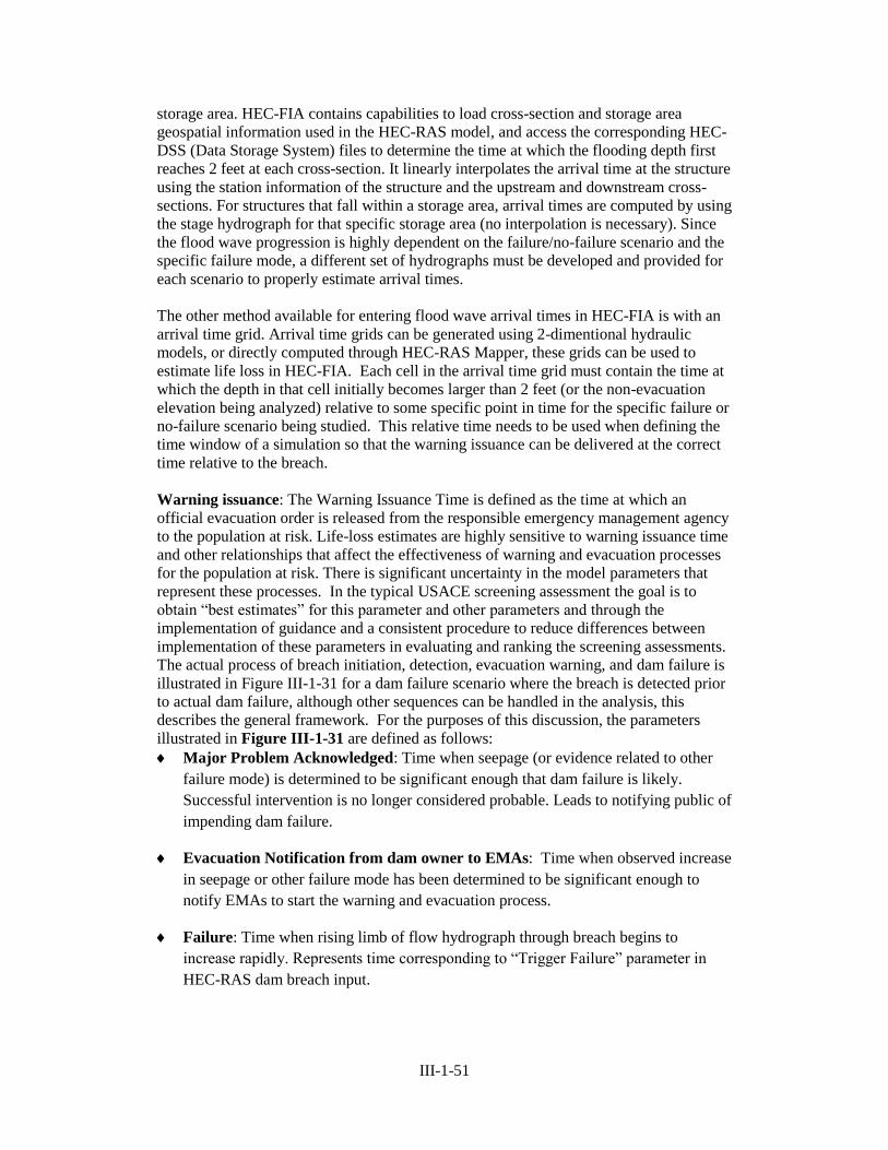
III-1-51

storage area. HEC-FIA contains capabilities to load cross-section and storage area

geospatial information used in the HEC-RAS model, and access the corresponding HEC-

DSS (Data Storage System) files to determine the time at which the flooding depth first

reaches 2 feet at each cross-section. It linearly interpolates the arrival time at the structure

using the station information of the structure and the upstream and downstream cross-

sections. For structures that fall within a storage area, arrival times are computed by using

the stage hydrograph for that specific storage area (no interpolation is necessary). Since

the flood wave progression is highly dependent on the failure/no-failure scenario and the

specific failure mode, a different set of hydrographs must be developed and provided for

each scenario to properly estimate arrival times.

The other method available for entering flood wave arrival times in HEC-FIA is with an

arrival time grid. Arrival time grids can be generated using 2-dimentional hydraulic

models, or directly computed through HEC-RAS Mapper, these grids can be used to

estimate life loss in HEC-FIA. Each cell in the arrival time grid must contain the time at

which the depth in that cell initially becomes larger than 2 feet (or the non-evacuation

elevation being analyzed) relative to some specific point in time for the specific failure or

no-failure scenario being studied. This relative time needs to be used when defining the

time window of a simulation so that the warning issuance can be delivered at the correct

time relative to the breach.

Warning issuance: The Warning Issuance Time is defined as the time at which an

official evacuation order is released from the responsible emergency management agency

to the population at risk. Life-loss estimates are highly sensitive to warning issuance time

and other relationships that affect the effectiveness of warning and evacuation processes

for the population at risk. There is significant uncertainty in the model parameters that

represent these processes. In the typical USACE screening assessment the goal is to

obtain “best estimates” for this parameter and other parameters and through the

implementation of guidance and a consistent procedure to reduce differences between

implementation of these parameters in evaluating and ranking the screening assessments.

The actual process of breach initiation, detection, evacuation warning, and dam failure is

illustrated in Figure III-1-31 for a dam failure scenario where the breach is detected prior

to actual dam failure, although other sequences can be handled in the analysis, this

describes the general framework. For the purposes of this discussion, the parameters

illustrated in Figure III-1-31 are defined as follows:

Major Problem Acknowledged: Time when seepage (or evidence related to other

failure mode) is determined to be significant enough that dam failure is likely.

Successful intervention is no longer considered probable. Leads to notifying public of

impending dam failure.

Evacuation Notification from dam owner to EMAs: Time when observed increase

in seepage or other failure mode has been determined to be significant enough to

notify EMAs to start the warning and evacuation process.

Failure: Time when rising limb of flow hydrograph through breach begins to

increase rapidly. Represents time corresponding to “Trigger Failure” parameter in

HEC-RAS dam breach input.

III-1-52

Warning Opportunity Time Window: Amount of time between when the dam

owner discovers significant seepage progression that could lead to impending dam

failure and actual Failure. Positive value if significant evidence related to failure

mode is discovered prior to failure initiation, negative if after failure.

Breach formation time: Amount of time between Failure and when breach reaches

full width and depth. Corresponds to “Full Formation Time” parameter in HEC-RAS

dam breach data.

Figure III-1-31. Detection and warning timeline for observed seepage failure

scenario

For most failure modes where the failure progress is observable prior to catastrophic

failure of the dam, warning issuance times should be determined by first estimating the

time when a major problem would be acknowledged relative to the time of dam failure.

The major problem acknowledgment time for these failure modes is the time at which a

dam owner would determine that a failure is likely imminent and they would decide that

the dam breach warning and evacuation process should be initiated by notifying the

responsible authorities. The time lag between major problem acknowledgement and when

an evacuation order would pass from the dam owner to the responsible emergency

agency (EMA) and then from the EMA to the public (Warning Issuance Time) should be

estimated based on the judgment of dam operations personnel and emergency

management personnel who have jurisdiction in the areas of each downstream

community. In obtaining input from operations personnel and emergency management

personnel it is important to carefully describe the dam-failure scenario, including the key

assumptions that define the development and detection of the failure mode that is

considered in each failure event-exposure scenario for which life loss is being estimated,

so that they can consider all associated factors in estimating warning issuance times for

structures. It is useful to have more than one responsible person involved in this expert

elicitation process since different individuals will often think of different important

factors and their judgments may vary resulting in a range of estimates of warning

issuance times. The process will often result in new ideas for reducing warning issuance

times. If a Potential Failure Mode Analysis is being performed, the warning issuance

times should be estimated by the group during discussion relevant to each failure mode.

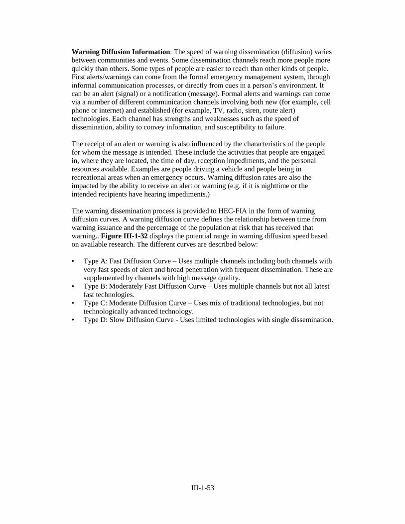
III-1-53

Warning Diffusion Information: The speed of warning dissemination (diffusion) varies

between communities and events. Some dissemination channels reach more people more

quickly than others. Some types of people are easier to reach than other kinds of people.

First alerts/warnings can come from the formal emergency management system, through

informal communication processes, or directly from cues in a person’s environment. It

can be an alert (signal) or a notification (message). Formal alerts and warnings can come

via a number of different communication channels involving both new (for example, cell

phone or internet) and established (for example, TV, radio, siren, route alert)

technologies. Each channel has strengths and weaknesses such as the speed of

dissemination, ability to convey information, and susceptibility to failure.

The receipt of an alert or warning is also influenced by the characteristics of the people

for whom the message is intended. These include the activities that people are engaged

in, where they are located, the time of day, reception impediments, and the personal

resources available. Examples are people driving a vehicle and people being in

recreational areas when an emergency occurs. Warning diffusion rates are also the

impacted by the ability to receive an alert or warning (e.g. if it is nighttime or the

intended recipients have hearing impediments.)

The warning dissemination process is provided to HEC-FIA in the form of warning

diffusion curves. A warning diffusion curve defines the relationship between time from

warning issuance and the percentage of the population at risk that has received that

warning.. Figure III-1-32 displays the potential range in warning diffusion speed based

on available research. The different curves are described below:

• Type A: Fast Diffusion Curve – Uses multiple channels including both channels with

very fast speeds of alert and broad penetration with frequent dissemination. These are

supplemented by channels with high message quality.

• Type B: Moderately Fast Diffusion Curve – Uses multiple channels but not all latest

fast technologies.

• Type C: Moderate Diffusion Curve – Uses mix of traditional technologies, but not

technologically advanced technology.

• Type D: Slow Diffusion Curve - Uses limited technologies with single dissemination.

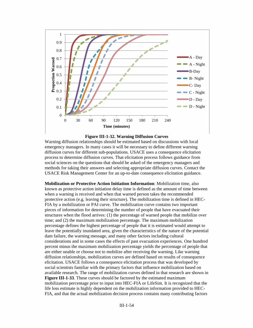
III-1-54

Figure III-1-32. Warning Diffusion Curves

Warning diffusion relationships should be estimated based on discussions with local

emergency managers. In many cases it will be necessary to define different warning

diffusion curves for different sub-populations. USACE uses a consequence elicitation

process to determine diffusion curves. That elicitation process follows guidance from

social sciences on the questions that should be asked of the emergency managers and

methods for taking their answers and selecting appropriate diffusion curves. Contact the

USACE Risk Management Center for an up-to-date consequence elicitation guidance.

Mobilization or Protective Action Initiation Information: Mobilization time, also

known as protective action initiation delay time is defined as the amount of time between

when a warning is received and when that warned person takes the recommended

protective action (e.g. leaving their structure). The mobilization time is defined in HEC-

FIA by a mobilization or PAI curve. The mobilization curve contains two important

pieces of information for determining the number of people that have evacuated their

structures when the flood arrives: (1) the percentage of warned people that mobilize over

time; and (2) the maximum mobilization percentage. The maximum mobilization

percentage defines the highest percentage of people that it is estimated would attempt to

leave the potentially inundated area, given the characteristics of the nature of the potential

dam failure, the warning message, and many other factors including cultural

considerations and in some cases the effects of past evacuation experiences. One hundred

percent minus the maximum mobilization percentage yields the percentage of people that

are either unable or choose not to mobilize after receiving the warning. Like warning

diffusion relationships, mobilization curves are defined based on results of consequence

elicitation. USACE follows a consequence elicitation process that was developed by

social scientists familiar with the primary factors that influence mobilization based on

available research. The range of mobilization curves defined in that research are shown in

Figure III-1-33. These curves should be factored by the estimated maximum

mobilization percentage prior to input into HEC-FIA or LifeSim. It is recognized that the

life loss estimate is highly dependent on the mobilization information provided to HEC-

FIA, and that the actual mobilization decision process contains many contributing factors

0

0.1

0.2

0.3

0.4

0.5

0.6

0.7

0.8

0.9

1

0 30 60 90 120 150 180 210 240

Pro

po

rtio

n W

arn

ed

Time (minutes)

A - Day

A - Night

B-Day

B- Night

C- Day

C - Night

D - Day

D - Night

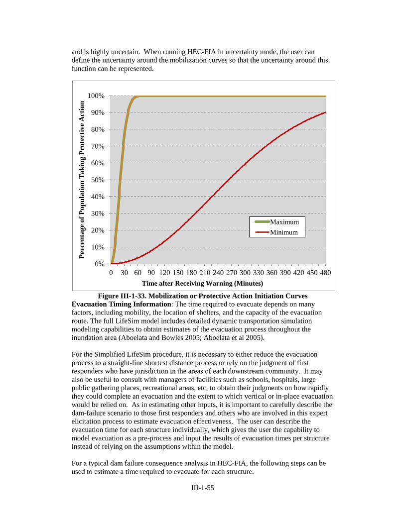
III-1-55

and is highly uncertain. When running HEC-FIA in uncertainty mode, the user can

define the uncertainty around the mobilization curves so that the uncertainty around this

function can be represented.

Figure III-1-33. Mobilization or Protective Action Initiation Curves

Evacuation Timing Information: The time required to evacuate depends on many

factors, including mobility, the location of shelters, and the capacity of the evacuation

route. The full LifeSim model includes detailed dynamic transportation simulation

modeling capabilities to obtain estimates of the evacuation process throughout the

inundation area (Aboelata and Bowles 2005; Aboelata et al 2005).

For the Simplified LifeSim procedure, it is necessary to either reduce the evacuation

process to a straight-line shortest distance process or rely on the judgment of first

responders who have jurisdiction in the areas of each downstream community. It may

also be useful to consult with managers of facilities such as schools, hospitals, large

public gathering places, recreational areas, etc, to obtain their judgments on how rapidly

they could complete an evacuation and the extent to which vertical or in-place evacuation

would be relied on. As in estimating other inputs, it is important to carefully describe the

dam-failure scenario to those first responders and others who are involved in this expert

elicitation process to estimate evacuation effectiveness. The user can describe the

evacuation time for each structure individually, which gives the user the capability to

model evacuation as a pre-process and input the results of evacuation times per structure

instead of relying on the assumptions within the model.

For a typical dam failure consequence analysis in HEC-FIA, the following steps can be

used to estimate a time required to evacuate for each structure.

0%

10%

20%

30%

40%

50%

60%

70%

80%

90%

100%

0 30 60 90 120 150 180 210 240 270 300 330 360 390 420 450 480

Per

cen

tage o

f P

op

ula

tion

Ta

kin

g P

rote

ctiv

e A

ctio

n

Time after Receiving Warning (Minutes)

Maximum

Minimum

III-1-56

1) Assume the safe location is anywhere that the maximum inundated depth for a given

flood scenario is less than 2 feet. Create a polygon representing this hazard boundary.

2) Load the hazard boundary into HEC-FIA and provide a nominal speed at which

evacuating people could travel along the assumed straight-line distance. This nominal

speed is less than the actual speed along the road network because the distance is

greater through the road network than along a straight-line path as represented in

Simplified LifeSim.

3) HEC-FIA will compute the time required to evacuate by determining the distance

from each structure to the safe boundary and then dividing that distance by the

nominal speed.

Lethality Zone Parameters and Fatality Rates: Flood (lethality) zones distinguish

physical flood environments in which historical rates of life loss have distinctly differed.

The LifeSim research resulted in three flood zones for which historical rates of life loss

were estimated and these fatality rates are used in HEC-FIA to estimate life loss. Each

flood zone is physically defined by the interplay between available shelter and local flood

depths and velocities, as summarized below:

Chance Zones: in which flood victims are typically swept downstream or trapped

underwater, and survival depends largely on chance; that is, the apparently random

occurrence of floating debris that can be clung to, getting washed to shore, or

otherwise finding refuge safely. The historical fatality rate in Chance Zones ranges

from about 38 percent to 100 percent, with an average rate over III-11 percent.

Compromised Zones: in which the available shelter has been severely damaged by

the flood, increasing the exposure of flood victims to violent floodwaters. An

example might be when the front of a house is torn away, exposing the rooms inside

to flooding. The historical fatality rate in Compromised Zones ranges from zero to

about 50 percent, with an average rate near 12 percent.

Safe Zones: which are typically dry, exposed to relatively quiescent floodwaters, or

exposed to shallow flooding unlikely to sweep people off their feet. Depending on

the nature of the flood, examples might include the second floor of residences and

sheltered backwater regions. Fatality rate in Safe Zones is virtually zero and

averages 0.02 percent.

As mentioned previously, the Simplified LifeSim approach in HEC-FIA uses velocity to

determine if a structure is capable of surviving the flood event. Therefore, assignment to

a specific lethality zone for a given structure is based on the maximum instantaneous

depth times velocity for survivorship and final depth of flooding at that structure given its

ability to provide safe haven, and the height of that structure. By including the height of

the structure, the very significant impact of vertical evacuation is accounted for in the

Simplified LifeSim methodology.

HEC-FIA assigns lethality zones based on the evacuation outcome for people starting in

each structure and the height of the structure. The logic followed by HEC-FIA for

III-1-57

assignment of evacuation outcome categories is described below. After the determination

of evacuation outcome is made, then lethality zones are determined. Certain parameters

in the lethality zone assignment process are set by default in HEC-FIA, but should be

reviewed during the application process to insure that they are representative of the study

area region:

1) Cleared: the people that evacuate safely do not receive a flood lethality zone

assignment.

2) Caught: the people that get caught evacuating are assigned to the Chance Zone.

3) Not mobilized: the people that stay in structures are assigned to flood lethality zones

based on maximum instantaneous depth times velocity, maximum depth of flooding

over the entire flood event and the height of the structure. The assumption in

Simplified LifeSim is that people evacuate to the level above the highest habitable

level in the structure (e.g. the roof or an attic).

a) For any structure: if the depth times velocity exceeds the RESCDam criteria for

partial survivorship, the structure will receive either chance or compromised

given maximum depth, if the depth times velocity exceeds the RESCDam criteria

for total destruction, the category is automatically determined to be Chance.

b) For any structure: if structure totally survives and event maximum depth < 2 feet

or less than the first floor height (fh) of structure, then no flood lethality zone

assignment is made and the people are grouped with the Cleared evacuation

category;

c) If 1-story structure where the population is under 65:

i) if the structure totally survives and event maximum depth < fh + 13 feet then

assign to Safe Zone, if structure partially survives, and maximum depth < fh

+13 ft then assign to compromised zone, if structure is totally destroyed, then

assign to chance zone:

ii) if the structure totally survives or partially survives the event and event

maximum depth ≥ fh + 13 feet and < fh + 15 feet then assign to a

Compromised Zone, if the structure is totally destroyed, then assign to

chance zone;

iii) else event maximum depth ≥ fh + 15 feet then assign to a Chance Zone.

d) For each additional story, add 9-1 feet to the depth criteria in b) to determine

flood lethality zone. Depending on occupancy type the fatality rates for over 65

the lethality zone thresholds can be set lower.

In the Simplified LifeSim Procedure the following average fatality rates are used based

on the probability distributions of fatality rates for each Flood Lethality Zone:

Safe Flood Zone: 0.0002

III-1-58

Compromised Flood Zone: 0.12

Chance Flood Zone: 0.91.

The entire probability distributions of fatality rates for each Flood Lethality Zone are

used in HEC-FIA when the uncertainty analysis option is selected.

Simplified LifeSim Methodology The Simplified LifeSim methodology applied within the HEC-FIA program includes the

following steps for a selected Event-Exposure Scenario and given structure inventory

with population to estimate loss of life. The steps below are illustrated in Figure III-1-

34.

1) Obtain the dam-failure flood wave arrival times for each structure. The arrival

time is the time at which the depth of flooding at the location of the structure is

estimated to be large enough that the inhabitants of that structure will choose to stay

in the structure and evacuate vertically instead of risk leaving the structure. The

default value in HEC-FIA is 2 feet. HEC-FIA estimates arrival times for each

structure by interpolating them off of the hydrograph data provided at the nearest

upstream and downstream location or by selecting it from the arrival time grid in the

specific cell where the structure is located.

2) Calculate the warning time for each structure by finding the difference between their

respective dam-failure flood wave arrival times (from Step 1) and the public warning

issuance time. Warning time indicates the amount of time that the population of each

structure has to receive a warning and mobilize, and through the warning diffusion

curve determine the percent of the population that was warned.

3) Compute the time required to evacuate for each structure, which is an estimate of

the amount of time it would take for the people in a structure to evacuate to a safe

location after they have mobilized.

4) Combine the user defined warning and mobilization curves into one relationship that

represents the number of people who have both received a warning and mobilized.

5) Compute the percentage of people in each Evacuation Outcome Category. For each

structure, estimate the percentage of its occupants that fall into to each of three

possible evacuation categories at the time of arrival of the dam-failure flood wave.

This estimate computes fractions of people in individual structures. When the results

are summed for the inundated area, it will provide an estimate of the total life risk for

the specific scenario.

6) For each structure, assign a lethality zone to the people in each evacuation outcome

category as described in the previous section.

7) Calculate the overall fatality rate for the occupants initially assigned to each

structure by summing the following fatality rates for each evacuation outcome

category

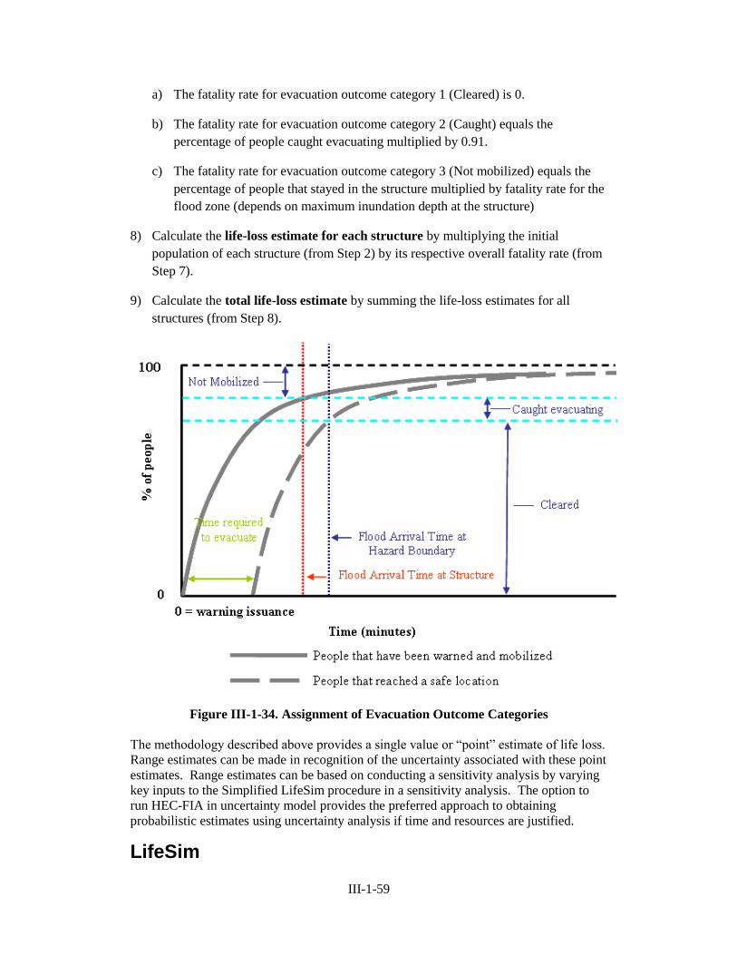
III-1-59

a) The fatality rate for evacuation outcome category 1 (Cleared) is 0.

b) The fatality rate for evacuation outcome category 2 (Caught) equals the

percentage of people caught evacuating multiplied by 0.91.

c) The fatality rate for evacuation outcome category 3 (Not mobilized) equals the

percentage of people that stayed in the structure multiplied by fatality rate for the

flood zone (depends on maximum inundation depth at the structure)

8) Calculate the life-loss estimate for each structure by multiplying the initial

population of each structure (from Step 2) by its respective overall fatality rate (from

Step 7).

9) Calculate the total life-loss estimate by summing the life-loss estimates for all

structures (from Step 8).

Figure III-1-34. Assignment of Evacuation Outcome Categories

The methodology described above provides a single value or “point” estimate of life loss.

Range estimates can be made in recognition of the uncertainty associated with these point

estimates. Range estimates can be based on conducting a sensitivity analysis by varying

key inputs to the Simplified LifeSim procedure in a sensitivity analysis. The option to

run HEC-FIA in uncertainty model provides the preferred approach to obtaining

probabilistic estimates using uncertainty analysis if time and resources are justified.

LifeSim

III-1-60

The full version of LifeSim is applied to support risk assessments within USACE when

the simplifying assumptions inherent in HEC-FIA result in too much uncertainty in the

life loss estimate. Also, given the detailed evacuation modeling available in LifeSim, it is

also applied to assist with evacuation planning. Many of the concepts described within

the HEC-FIA section above are also applicable within the LifeSim methodology

(Lethality Zones, Fatality Rates, etc).

As stated previously, the main difference between the simplified LifeSim approach in

HEC-FIA and the full LifeSim methodology is the evacuation modeling. Simplified

LifeSim uses a basic evacuation model where the user either provides the amount of time

required for inhabitants of each structure to evacuate to safety or provides a hazard

boundary in the form of a polygon shapefile. If a hazard boundary is provided, HEC-FIA

determines the shortest straight-line distance from a structure to the hazard boundary and

applies a nominal evacuation speed along that line to estimate the amount of time

required to evacuate. The effect of traffic jam potential must be accounted for implicitly

by the choice of the nominal evacuation speed. If the loss of life for a study is highly

dependent on evacuation efficiency, including the effects of traffic congestion,

application of the full version of LifeSim should be considered as it contains a more

detailed evacuation model.

LifeSim uses an agent-based approach to track individuals throughout the warning and

evacuation process. It also contains a traffic simulation engine to simulate the evacuation

process that allows vehicles to interact with other vehicles and the hazard. The

computation engine offers an effective estimation of population re-distribution during the

evacuation process. LifeSim was developed with an uncertainty sampling approach. By

sampling uncertain parameters and running the model iteratively, LifeSim is capable of

producing a distribution of results to better inform a risk assessment.

It is important to note that LifeSim is simulating the entire warning, mobilization, and

evacuation process. The process can be illustrated with the following example. Consider

a single family home containing 3 people that is located in the study area for a given

simulation. Once a flood warning is issued by emergency managers, it takes some

amount of time before a resident in the home receives the warning. Once the warning is

received and understood at the home, the family members will take some time to gather

their belongings and prepare for leaving their home. The family then leaves their home

in a car containing 3 people. On the road, they interact with both other vehicles on the

road and flood waters. For example, they may encounter a traffic jam at a freeway on-

ramp and choose a different route out of the hazard area (see Figure 1). Or they may

choose to tough it out in the traffic jam, hoping that it will clear up. If the family reaches

a road that is currently flooded they can attempt to turn around and go in a different

direction. If the family gets caught on a flooded road, the survival of each family

member is dependent on their state (e.g. age) and the hydraulic conditions at their

location. All of these interactions are simulated during an LifeSim model iteration.

Because warning times and people’s behavior are sampled from a range of possibilities,

the same family may take longer to get warned or choose to remain in their home during

the next model iteration.

Simulation results for existing conditions and alternatives can be visualized using

LifeSim animation capabilities. In the LifeSim results animation image shown in Figure

III-135, structures and cars caught (inundated) by floodwaters are red. Yellow structures

indicate that a warning was received but the people inside haven’t started evacuating yet,

and brown structures indicate that a warning hasn’t been received yet. Blue cars represent

III-1-61

people mobilizing on roads, and are tracked throughout the study area based on traffic

simulation algorithms.

By tracking individual people

and their movements, LifeSim

can help identify where people

are most at risk of losing their

lives, whether it is on roads or

in structures. We can now

pinpoint the locations of

greatest potential life loss,

which is useful when

developing alternative project

formulations. For example, a

simulation may show that life

loss on a particular road is

significant. LifeSim allows for

a detailed analysis of a range

of alternatives based on both

structural and nonstructural

measures for reducing potential

life loss. Nonstructural

measures to reduce life loss could include raising or closing at risk road embankments

and increasing road capacities to reduce congestion. A nonstructural alternative could

also consist of increasing the warning time through better warning issuance and

community awareness.

Rather than presenting the entire LifeSim methodology from a theoretical basis, which

would be largely repetitive from the simplified LifeSim approach described above, the

following example is used to illustrate the full version of LifeSim.

Example LifeSim Application

Introduction "Herbert Hoover Dike (HHD) is an earthen dam impounding Lake Okeechobee, the

nation’s second largest lake. HHD was constructed by hydraulic dredge and fill methods

by private and public entities between the early 1900’s and the late 1960’s, initially to

provide agricultural water supply. Following major hurricane disasters in 1926 and 1928,

Congress authorized USACE to construct elevated embankments at the north and south

of the Lake to provide flood protection. In the 1960’s, the Lake was completely encircled

with approximately 143 miles of dike and tie-back levees.

Prior to 1978, the Lake conservation pool was generally managed between 12.7 and 14.2

ft. (NAVD88). In 1978, the conservation pool was raised to 17.2 ft. (NAVD88) to meet

water supply needs. Indications of excessive seepage and piping were first noted

beginning in the early 1980’s. Conditions worsened with time, particularly following

years in which lake elevations alternated between extreme high and low levels. To

enhance the Lake ecology, and recognizing the risk imposed by the deteriorating

condition of the Dike, the Lake Okeechobee Regulation Schedule (LORS), implemented

in 2008, lowered the conservation pool upper limit to 15.95 ft. (NAVD88).

Figure III-135. Example LifeSim Animation

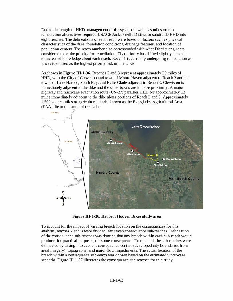
III-1-62

Due to the length of HHD, management of the system as well as studies on risk

remediation alternatives required USACE Jacksonville District to subdivide HHD into

eight reaches. The delineations of each reach were based on factors such as physical

characteristics of the dike, foundation conditions, drainage features, and location of

population centers. The reach number also corresponded with what District engineers

considered to be the priority for remediation. That priority has shifted slightly since due

to increased knowledge about each reach. Reach 1 is currently undergoing remediation as

it was identified as the highest priority risk on the Dike.

As shown in Figure III-1-36, Reaches 2 and 3 represent approximately 30 miles of

HHD, with the City of Clewiston and town of Moore Haven adjacent to Reach 2 and the

towns of Lake Harbor, South Bay, and Belle Glade adjacent to Reach 3. Clewiston is

immediately adjacent to the dike and the other towns are in close proximity. A major

highway and hurricane evacuation route (US-27) parallels HHD for approximately 12

miles immediately adjacent to the dike along portions of Reach 2 and 3. Approximately

1,500 square miles of agricultural lands, known as the Everglades Agricultural Area

(EAA), lie to the south of the Lake.

Figure III-1-36. Herbert Hoover Dikes study area

To account for the impact of varying breach location on the consequences for this

analysis, reaches 2 and 3 were divided into seven consequence sub-reaches. Delineation

of the consequence sub-reaches was done so that any breach within each sub-reach would

produce, for practical purposes, the same consequence. To that end, the sub-reaches were

delineated by taking into account consequence centers (developed city boundaries from

areal imagery), topography, and major flow impediments. The actual location of the

breach within a consequence sub-reach was chosen based on the estimated worst-case

scenario. Figure III-1-37 illustrates the consequence sub-reaches for this study.

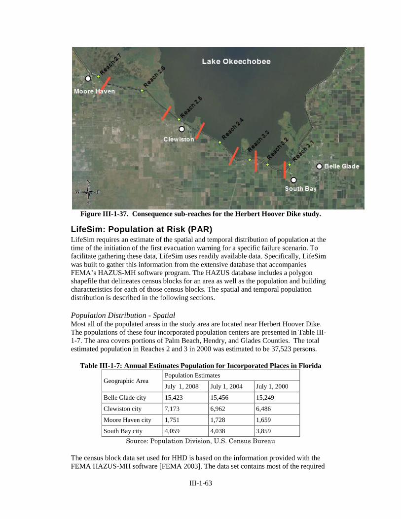
III-1-63

Figure III-1-37. Consequence sub-reaches for the Herbert Hoover Dike study.

LifeSim: Population at Risk (PAR) LifeSim requires an estimate of the spatial and temporal distribution of population at the

time of the initiation of the first evacuation warning for a specific failure scenario. To

facilitate gathering these data, LifeSim uses readily available data. Specifically, LifeSim

was built to gather this information from the extensive database that accompanies

FEMA’s HAZUS-MH software program. The HAZUS database includes a polygon

shapefile that delineates census blocks for an area as well as the population and building

characteristics for each of those census blocks. The spatial and temporal population

distribution is described in the following sections.

Population Distribution - Spatial Most all of the populated areas in the study area are located near Herbert Hoover Dike.

The populations of these four incorporated population centers are presented in Table III-

1-7. The area covers portions of Palm Beach, Hendry, and Glades Counties. The total

estimated population in Reaches 2 and 3 in 2000 was estimated to be 37,523 persons.

Table III-1-7: Annual Estimates Population for Incorporated Places in Florida

Geographic Area Population Estimates

July 1, 2008 July 1, 2004 July 1, 2000

Belle Glade city 15,423 15,456 15,249

Clewiston city 7,173 6,962 6,486

Moore Haven city 1,751 1,728 1,659

South Bay city 4,059 4,038 3,859

Source: Population Division, U.S. Census Bureau

The census block data set used for HHD is based on the information provided with the

FEMA HAZUS-MH software [FEMA 2003]. The data set contains most of the required

III-1-64

population and demographic information required to run LifeSim. HAZUS database

version 1.3 was used in for this analysis. A subsequent release (version 1.4) of the

database was made by FEMA midway through the study. Inputs for this specific study

area were compared between the two versions, and no appreciable differences were

discovered.

For each breach location, only those census blocks that were inundated within the first 20

hours after breach were included in the LifeSim model for a given scenario. The

assumption is that after 20 hours, all PAR in the potential inundation zone that would

otherwise be unable or choose not to evacuate would be assisted or convinced to leave

their residence. Emergency planning zone (EPZ) fields were added to the default HAZUS

database to meet requirements of the LifeSim software. The EPZ field allows LifeSim to

indentify different warning and mobilization relationships for communities in the flooded

area.

Populations were adjusted from the default year 2000 populations provided in the

HAZUS database to 2008 estimates from the University of Florida Bureau of Economic

and Business Research. Adjustments were made on a community-by-community basis by

multiplying the population in all census blocks located in a community by the appropriate

factor to reach the year 2008 estimates for that community.

Migrant worker information was provided by Jacksonville District for Hendry and Palm

Beach counties. The information included migrant housing locations and capacities.

These values were added to the night time (2 am) residential population for the census

block where they are located. For daytime, migrant populations were spread evenly to

census blocks within the study area that contained agricultural fields which were

identified using areal imagery. A total of 4,741 migrant workers were added to the day

and night census information for Hendry and Palm Beach counties.

For all flood scenarios where the breach occurs at or above 20 ft. NAVD88, the starting

population for all census blocks was reduced by 30%. This pre-breach evacuation

assumption is based on the following statement from the HHD Emergency Action Plan

(June 2008): “If EL 21.5 ft. NGVD29 is reached without rehabilitation, recent

engineering studies indicate that failure would be certain” (Elevation 21.5 ft. NGVD29 is

equal to 20.2 ft. NAVD88.). Hence, we assumed that an evacuation order would be in

effect until the lake level dropped back below EL 20 ft. NAVD88.

The value of 30% for the pre-breach evacuation is based on various sources of

information. The Palm Beach County HHD Emergency Evacuation Guidance Document

(PBCDEM 2006) states that “It is projected that approximately 40-70 percent may

comply with a mandatory evacuation order when issued prior to a hurricane.” The mean

of this value was originally chosen because no further information was available.

However, there was some concern that this number might not be realistic for Glades and

Henry Counties. The socioeconomic and demographic characteristics of those counties

are significantly different than Palm Beach County, and even the communities within

Palm Beach County that are affected by HHD are not representative of the majority of

that county. Therefore, additional information was obtained through interviews with

local and county emergency responders and city officials in the towns of Clewiston and

Belle Glade. They provided estimates between 5% (Clewiston) and 40% (Belle Glade)

for the number of people that would leave if given an evacuation order related to

imminent failure of HHD. Due to the relevant local experience and expertise of these

III-1-65

officials, the team considered that a number in the range of 5% and 40% would be a more

realistic estimate of the pre-evacuation response rate. As a result of this information and

the previously documented information, 30% was selected as the most realistic average

estimate of the pre-breach evacuation response rate.

Population Distribution – Temporal Variations in the number of people within the flooded area throughout the day can have a

significant effect on loss of life. Moreover, the activities that people are engaged in can

affect the efficiency at which the warning spreads through an area. Accordingly, LifeSim

is designed to take into account both 1) the distribution of people among census blocks

throughout the inundated area based on time of day and 2) estimates in the percentage of

population involved in various activity types including: at home, outdoors,

working/shopping and in transit.

To capture the variation in population and resulting variation in potential life loss at

different times of day, estimates of life loss were computed for breaches occurring at 12

different times of day for this study. The 12 times of day used were midnight, 0200,

0400, 0600, etc. To determine the number of people in a census block at any given time,

LifeSim pulls relevant data from the HAZUS-MH database. The HAZUS-MH database

contains three time-of-day activity distributions. These distributions are as follows: 0200,

representing night time; 1400, representing day time; and 1700, representing commuting

time. LifeSim takes the data and uses relationships to calculate the number of people in

each occupancy class on the census block level.

Variables used in distributing people are as follows:

Census block population taken from census data stored in HAZUS-MH database

Daytime residential population inferred from census data

Nighttime residential population inferred from census data

Number of people commuting inferred from census data

Number of people employed in the commercial sector

Number of people employed in the industrial sector

Number of students in grade schools (K-12)

Number of students on college and university campuses in the census tract

Number of people staying in hotels in the census tract

A factor representing the proportion of commuters using automobiles, inferred

from profile of the community (0.60 for dense urban, 0.80 for less dense urban or

suburban, and 0.85 for rural). The HAZUS-MH default value is 0.80.

Number of regional residents who do not live in the study area, visiting the

census tract for shopping and entertainment. The HAZUS-MH default value is

zero.

LifeSim interpolates the estimates obtained by applying the HAZUS-MH population data

for the three HAZUS-MH time-of-day distributions to obtain estimates for every two-

hour interval throughout a 24-hour period. Figure III-1-38 illustrates the fluctuation of

population at risk within the 20-hour inundation boundary for a breach in consequence

sub-reach 2 point 5. (Breaches at pool elevations of 14 ft. and 17 ft. NAVD88 do not

cause inundation of populated areas, hence the 0 population at risk for those elevations.)

This temporal distribution suggests that a large percentage of the population leaves the

area during the day and returns at night.

III-1-66

Figure III-1-38. Population distribution by time of day for breach at reach 2

point 5.

Population estimates for each of the four LifeSim activity types are then

computed using the mapping shown in Table III-1-8.

Table III-1-8. Mapping of HAZUS-MH occupancy classes to LifeSim activity types.

LifeSim activity type HAZUS occupancy class

Residential-indoors Residential-indoors

Hotels-indoors

Outdoors Residential-outdoors

Hotels-outdoors

Working/shopping Commercial-indoors

Commercial-outdoors

Industrial-indoors

industrial-outdoors

Education-indoors

Education-outdoors

In transit Commuting-own car

Commuting-public transportation

Finally, population is distributed among activity types using a set of activity factors.

These values are based on research from research by Rogers and Sorensen in 1988. Their

research described how a given warning system has a penetration capability that can be

distinguished for the following five fundamental locations or activities:

1. Home asleep

2. Indoors at home or in the neighborhood

3. Outdoors in the neighborhood

4. In transit

5. Working or shopping

0

2000

4000

6000

8000

10000

12000

12

:00

AM

2:0

0 A

M

4:0

0 A

M

6:0

0 A

M

8:0

0 A

M

10

:00

AM

12

:00

PM

2:0

0 P

M

4:0

0 P

M

6:0

0 P

M

8:0

0 P

M

10

:00

PM

Pop

ula

tion

at

Ris

k

Breach Time

30' (30% Pre-evac.)

25' (30% Pre-evac.)

20' (No Pre-evac.)

20' (30% Pre-evac.)

17' (No Pre-evac.)

14' (No Pre-evac.)

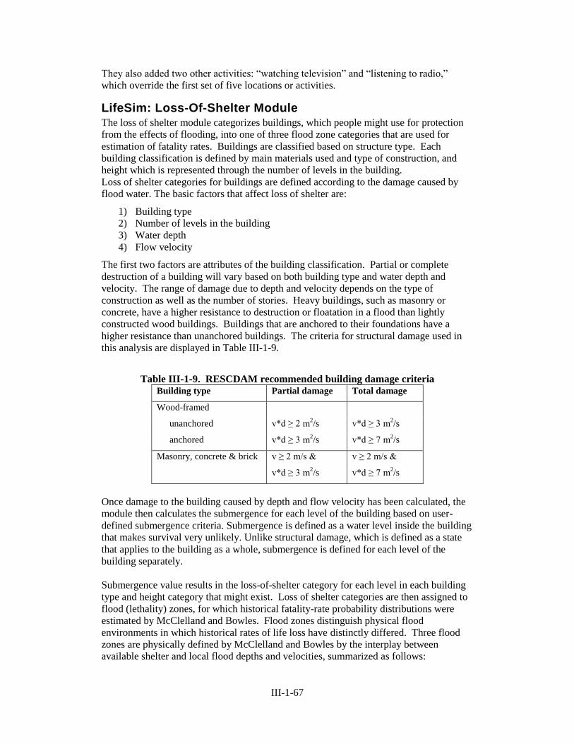
III-1-67

They also added two other activities: “watching television” and “listening to radio,”

which override the first set of five locations or activities.

LifeSim: Loss-Of-Shelter Module The loss of shelter module categorizes buildings, which people might use for protection

from the effects of flooding, into one of three flood zone categories that are used for

estimation of fatality rates. Buildings are classified based on structure type. Each

building classification is defined by main materials used and type of construction, and

height which is represented through the number of levels in the building.

Loss of shelter categories for buildings are defined according to the damage caused by

flood water. The basic factors that affect loss of shelter are:

1) Building type

2) Number of levels in the building

3) Water depth

4) Flow velocity

The first two factors are attributes of the building classification. Partial or complete

destruction of a building will vary based on both building type and water depth and

velocity. The range of damage due to depth and velocity depends on the type of

construction as well as the number of stories. Heavy buildings, such as masonry or

concrete, have a higher resistance to destruction or floatation in a flood than lightly

constructed wood buildings. Buildings that are anchored to their foundations have a

higher resistance than unanchored buildings. The criteria for structural damage used in

this analysis are displayed in Table III-1-9.

Table III-1-9. RESCDAM recommended building damage criteria Building type Partial damage Total damage

Wood-framed

unanchored v*d ≥ 2 m2/s v*d ≥ 3 m

2/s

anchored v*d ≥ 3 m2/s v*d ≥ 7 m

2/s

Masonry, concrete & brick v ≥ 2 m/s &

v*d ≥ 3 m2/s

v ≥ 2 m/s &

v*d ≥ 7 m2/s

Once damage to the building caused by depth and flow velocity has been calculated, the

module then calculates the submergence for each level of the building based on user-

defined submergence criteria. Submergence is defined as a water level inside the building

that makes survival very unlikely. Unlike structural damage, which is defined as a state

that applies to the building as a whole, submergence is defined for each level of the

building separately.

Submergence value results in the loss-of-shelter category for each level in each building

type and height category that might exist. Loss of shelter categories are then assigned to

flood (lethality) zones, for which historical fatality-rate probability distributions were

estimated by McClelland and Bowles. Flood zones distinguish physical flood

environments in which historical rates of life loss have distinctly differed. Three flood

zones are physically defined by McClelland and Bowles by the interplay between

available shelter and local flood depths and velocities, summarized as follows:

III-1-68

Chance zones in which flood victims are typically swept downstream or

trapped underwater and survival depends largely on chance; that is, the

apparently random occurrence of floating debris that can be clung to, getting

washed to shore, or otherwise finding refuge safely. Historical fatality rates

range from about 50 percent to 100 percent, with an average rate of about 90

percent.

Compromised zones in which the available shelter has been severely

damaged by the flood, increasing the exposure of flood victims to violent

floodwaters. An example might be when the rooms inside a building

experience rapidly-moving shoulder-height flood water. Historical fatality

rates range from zero to about 50 percent, with an average rate of about 10

percent.

Safe zones are typically dry, exposed to relatively quiescent floodwaters, or

exposed to shallow flooding unlikely to sweep people off their feet.

Examples might include the second floor of residences and sheltered

backwater regions. Historical fatality rates are virtually zero.

Debris in flood water can have a damaging effect on buildings, vehicles, and people.

However, the effects of debris are not explicitly considered in LifeSim.

For this analysis, the loss of life analysis was computed on a census block level. The

number of buildings in a census block is obtained from the HAZUS-MH data, which is

categorized into the different building types and numbers of levels. The loss of shelter

estimates are applied to the number of buildings in each building type under the

assumption that the buildings are uniformly distributed throughout a census block.

The submergence criteria for each level in a building used in this analysis are displayed

in Figure III-1-39 and Table III-1-10. LifeSim is setup to allow people below the age of

65 to climb to the highest level of residential buildings, which is the roof for all structure

types other than mobile homes. For people above the age of 65, LifeSim places them in

the highest level below the roof. (The number of PAR above age 65 is provided in the

HAZUS census data). For basements, submergence is considered to occur for any water

level above the ground surface. For non-residential buildings, LifeSim was set up to

allow people to move to the top floor, but not onto the roof. The first floor level is

determined based on typical foundation heights in the study area, while the levels of other

floors are estimated based on the first floor level and a standard floor height. Foundation

heights were set to 0 ft. (slab on grade) for all structures in this study as determined by

visual inspection (Google Earth Street View) and information from Jacksonville District.

In case of partial building damage, flood water can move into the building through a

knocked down wall or window. People inside the building are exposed to a flow of water

that might be capable of sweeping them out of the building into the open flood. Loss-of-

shelter category is decided in this case based on water depth and velocity inside each

level in the building compared to human stability criteria.

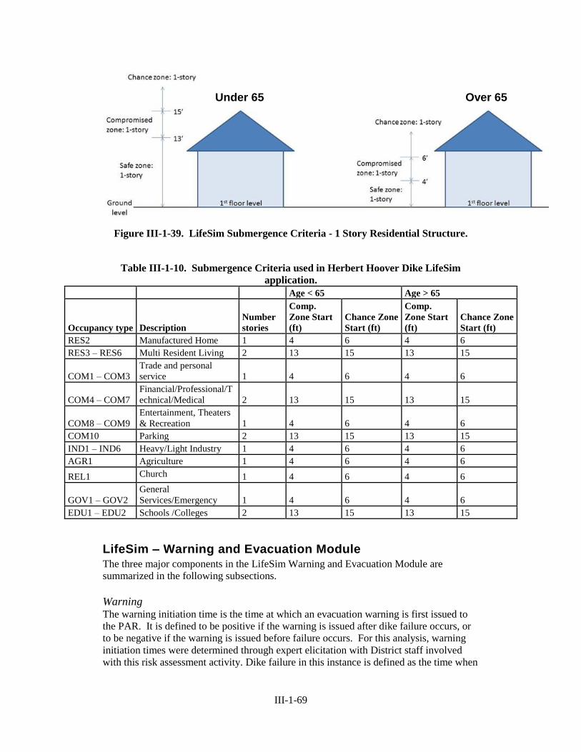
III-1-69

Figure III-1-39. LifeSim Submergence Criteria - 1 Story Residential Structure.

Table III-1-10. Submergence Criteria used in Herbert Hoover Dike LifeSim

application.

Age < 65 Age > 65

Occupancy type Description

Number

stories

Comp.

Zone Start

(ft)

Chance Zone

Start (ft)

Comp.

Zone Start

(ft)

Chance Zone

Start (ft)

RES2 Manufactured Home 1 4 6 4 6

RES3 – RES6 Multi Resident Living 2 13 15 13 15

COM1 – COM3

Trade and personal

service 1 4 6 4 6

COM4 – COM7

Financial/Professional/T

echnical/Medical 2 13 15 13 15

COM8 – COM9

Entertainment, Theaters

& Recreation 1 4 6 4 6

COM10 Parking 2 13 15 13 15

IND1 – IND6 Heavy/Light Industry 1 4 6 4 6

AGR1 Agriculture 1 4 6 4 6

REL1 Church 1 4 6 4 6

GOV1 – GOV2

General

Services/Emergency 1 4 6 4 6

EDU1 – EDU2 Schools /Colleges 2 13 15 13 15

LifeSim – Warning and Evacuation Module The three major components in the LifeSim Warning and Evacuation Module are

summarized in the following subsections.

Warning The warning initiation time is the time at which an evacuation warning is first issued to

the PAR. It is defined to be positive if the warning is issued after dike failure occurs, or

to be negative if the warning is issued before failure occurs. For this analysis, warning

initiation times were determined through expert elicitation with District staff involved

with this risk assessment activity. Dike failure in this instance is defined as the time when

Under 65 Over 65

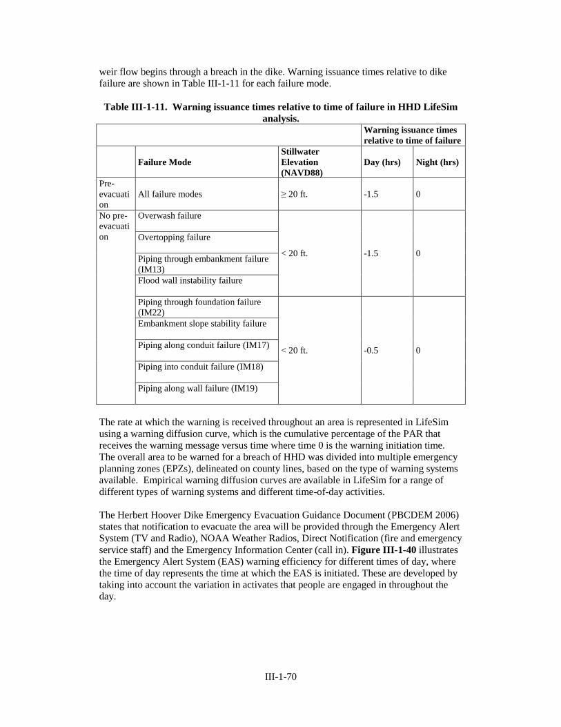
III-1-70

weir flow begins through a breach in the dike. Warning issuance times relative to dike

failure are shown in Table III-1-11 for each failure mode.

Table III-1-11. Warning issuance times relative to time of failure in HHD LifeSim

analysis. Warning issuance times

relative to time of failure

Failure Mode

Stillwater

Elevation

(NAVD88)

Day (hrs) Night (hrs)

Pre-

evacuati

on

All failure modes ≥ 20 ft. -1.5 0

No pre-

evacuati

on

Overwash failure

< 20 ft. -1.5 0

Overtopping failure

Piping through embankment failure

(IM13)

Flood wall instability failure

Piping through foundation failure

(IM22)

< 20 ft. -0.5 0

Embankment slope stability failure

Piping along conduit failure (IM17)

Piping into conduit failure (IM18)

Piping along wall failure (IM19)

The rate at which the warning is received throughout an area is represented in LifeSim

using a warning diffusion curve, which is the cumulative percentage of the PAR that

receives the warning message versus time where time 0 is the warning initiation time.

The overall area to be warned for a breach of HHD was divided into multiple emergency

planning zones (EPZs), delineated on county lines, based on the type of warning systems

available. Empirical warning diffusion curves are available in LifeSim for a range of

different types of warning systems and different time-of-day activities.

The Herbert Hoover Dike Emergency Evacuation Guidance Document (PBCDEM 2006)

states that notification to evacuate the area will be provided through the Emergency Alert

System (TV and Radio), NOAA Weather Radios, Direct Notification (fire and emergency

service staff) and the Emergency Information Center (call in). Figure III-1-40 illustrates

the Emergency Alert System (EAS) warning efficiency for different times of day, where

the time of day represents the time at which the EAS is initiated. These are developed by

taking into account the variation in activates that people are engaged in throughout the

day.

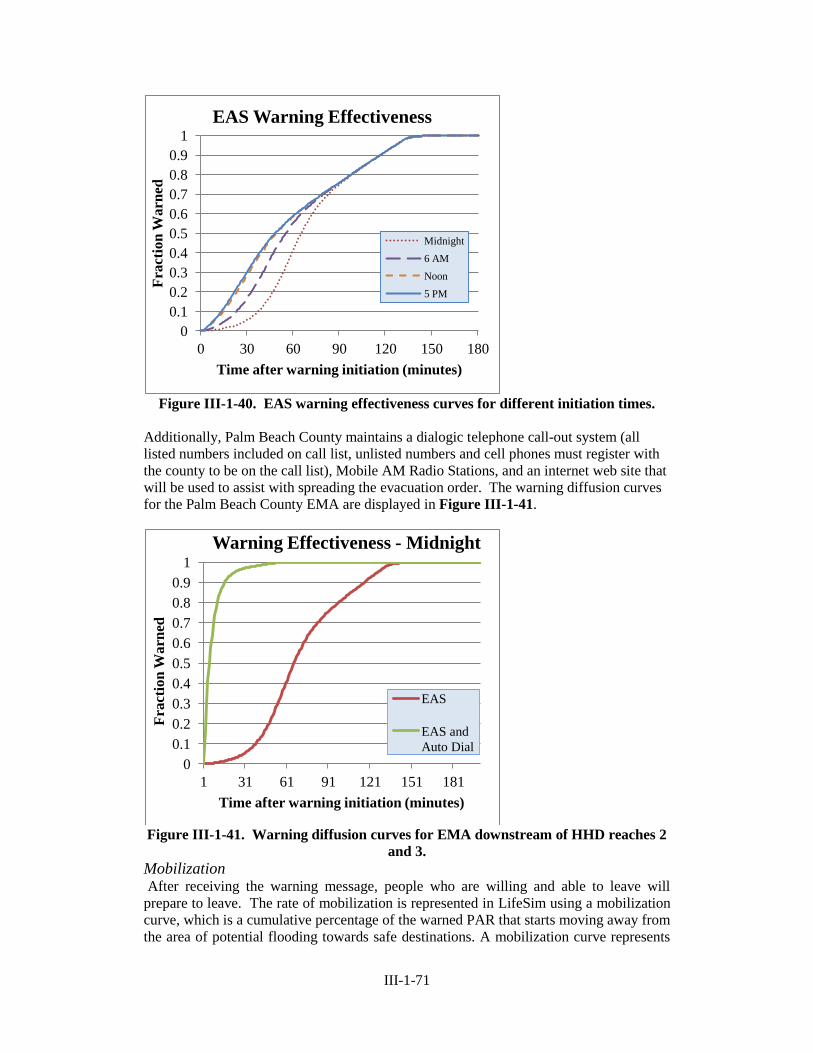
III-1-71

Figure III-1-40. EAS warning effectiveness curves for different initiation times.

Additionally, Palm Beach County maintains a dialogic telephone call-out system (all

listed numbers included on call list, unlisted numbers and cell phones must register with

the county to be on the call list), Mobile AM Radio Stations, and an internet web site that

will be used to assist with spreading the evacuation order. The warning diffusion curves

for the Palm Beach County EMA are displayed in Figure III-1-41.

Figure III-1-41. Warning diffusion curves for EMA downstream of HHD reaches 2

and 3.

Mobilization After receiving the warning message, people who are willing and able to leave will

prepare to leave. The rate of mobilization is represented in LifeSim using a mobilization

curve, which is a cumulative percentage of the warned PAR that starts moving away from

the area of potential flooding towards safe destinations. A mobilization curve represents

0

0.1

0.2

0.3

0.4

0.5

0.6

0.7

0.8

0.9

1

0 30 60 90 120 150 180

Fra

ctio

n W

arn

ed

Time after warning initiation (minutes)

EAS Warning Effectiveness

Midnight

6 AM

Noon

5 PM

0

0.1

0.2

0.3

0.4

0.5

0.6

0.7

0.8

0.9

1

1 31 61 91 121 151 181

Fra

ctio

n W

arn

ed

Time after warning initiation (minutes)

Warning Effectiveness - Midnight

EAS

EAS and

Auto Dial

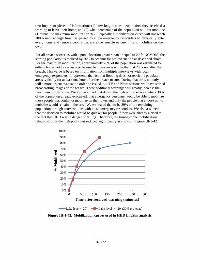
III-1-72

two important pieces of information: (1) how long it takes people after they received a

warning to leave their home, and (2) what percentage of the population will not mobilize

(1 minus the maximum mobilization %). Typically a mobilization curve will not reach

100% until enough time has passed to allow emergency responders to physically enter

every home and remove people that are either unable or unwilling to mobilize on their

own.

For all breach scenarios with a pool elevation greater than or equal to 20 ft. NGVD88, the

starting population is reduced by 30% to account for pre-evacuation as described above.

For the maximum mobilization, approximately 20% of the population was estimated to

either choose not to evacuate or be unable to evacuate within the first 20 hours after the

breach. This value is based on information from multiple interviews with local

emergency responders. It represents the fact that flooding does not reach the populated

areas typically for at least one hour after the breach occurs. During that time, not only

will a more urgent evacuation order be issued, but TV and News stations will have started

broadcasting images of the breach. These additional warnings will greatly increase the

maximum mobilization. We also assumed that during the high pool scenarios where 30%

of the population already evacuated, that emergency personnel would be able to mobilize

those people that could not mobilize on their own, and only the people that choose not to

mobilize would remain in the area. We estimated that to be 89% of the remaining

population through conversations with local emergency responders. We also assumed

that the decision to mobilize would be quicker for people if they were already alerted to

the fact that HHD was in danger of failing. Therefore, the timing of the mobilization

relationship for the high pools was reduced significantly as shown in Figure III-1-42.

Figure III-1-42. Mobilization curves used in HHD LifeSim analysis.

0%

10%

20%

30%

40%

50%

60%

70%

80%

90%

100%

0 50 100 150 200 250 300

% M

ob

iliz

ed

Time after received warning (minutes)

Lake level < 20' Lake level >= 20' (30% pre-evac)

III-1-73

Evacuation-Transportation The evacuation-transportation process commences with mobilization and ends with either

clearance of the flooding area or entrapment if the evacuation route becomes blocked by

flooding. People who clear the flooding area are assigned to a “safe” flood zone and

people who are trapped on the road are assigned to a flood zone that depends on their

mode of evacuation and the most severe flooding conditions for the event.

Three modes of evacuation are included in LifeSim: cars, sports utility vehicles (SUV’s)

and pedestrians. The following distribution of evacuation modes was determined through

discussions with USACE Jacksonville District staff: Passenger car (50%), Trucks (50%),

pedestrian (0%). 0% was chosen for pedestrian evacuation due to the large distances that

people would be required to cover to get to safety if HHD was to fail (i.e. no evacuation

destinations are inside the inundated areas and the inundated areas are extremely large).

LifeSim was also configured with the assumption that an average of three people would

occupy each evacuating vehicle.

The Greenshield [1935] transportation model is used in LifeSim to represent the effects

of traffic density and road capacity on vehicle speed. The original model was modified to

represent congestion and traffic jams by introducing a minimum “stop-and-go” speed

(Vjam) if the jam density (Djam) for a road class is exceeded. Each road class is

assigned default values of the number of lanes, free flow speed (ffs), Djam and Vjam

based on the Highway Capacity Manual (HCM) [TRB 2000], although these can be

overridden if more detailed information is available for the road system.

A GIS road network polyline shapefile was obtained from the USGS web site that

contained most roads in the area. It also contained the data required by LifeSim to

determine number of lanes, free-flow speed, jam density, and a minimum “stop and go”

speed. The USGS road network was modified on a case-by-case basis as necessary to

repair the original data when obvious errors were encountered that had a significant

impact on traffic movement during the evacuation process. Generally, missing road

segments were added by referencing areal imagery.

A GIS point shapefile represents a set of safe destinations for evacuees to go. LifeSim

models the movement of people to destination points using the shortest route available.

People who reach a safe destination are considered as the “cleared” group. Safe

destination locations were carefully defined to represent the expected evacuation situation

in each scenario. Designated routes in evacuation traffic management plans were used to

assess the likely evacuation routes. Evacuation destinations were placed just outside the

maximum inundated area on the main evacuation routes that would be used by people to

leave the flooded area. No evacuation destinations are located within the flooded area.

The actual shelters are located far away from the flooded area in most cases, and the

assumption is that people would proceed to those shelters after getting out of immediate

danger from the dike breach.

LifeSim – Loss-of-Life Module The final step in LifeSim is the estimation of loss of life. Previously described modules

simulate the spatial redistribution of people existing within the study area through the

processes of warning and evacuation and assign loss-of-shelter category/flood zones

based on the effect of flood water on the buildings, vehicles and pedestrians throughout

the study region. These results are combined in the Loss-of-Life (LOL) Module with the

probability distribution of fatality rates for each loss-of-shelter category/flood zone to

obtain estimates of the expected number of fatalities within the study area. For this

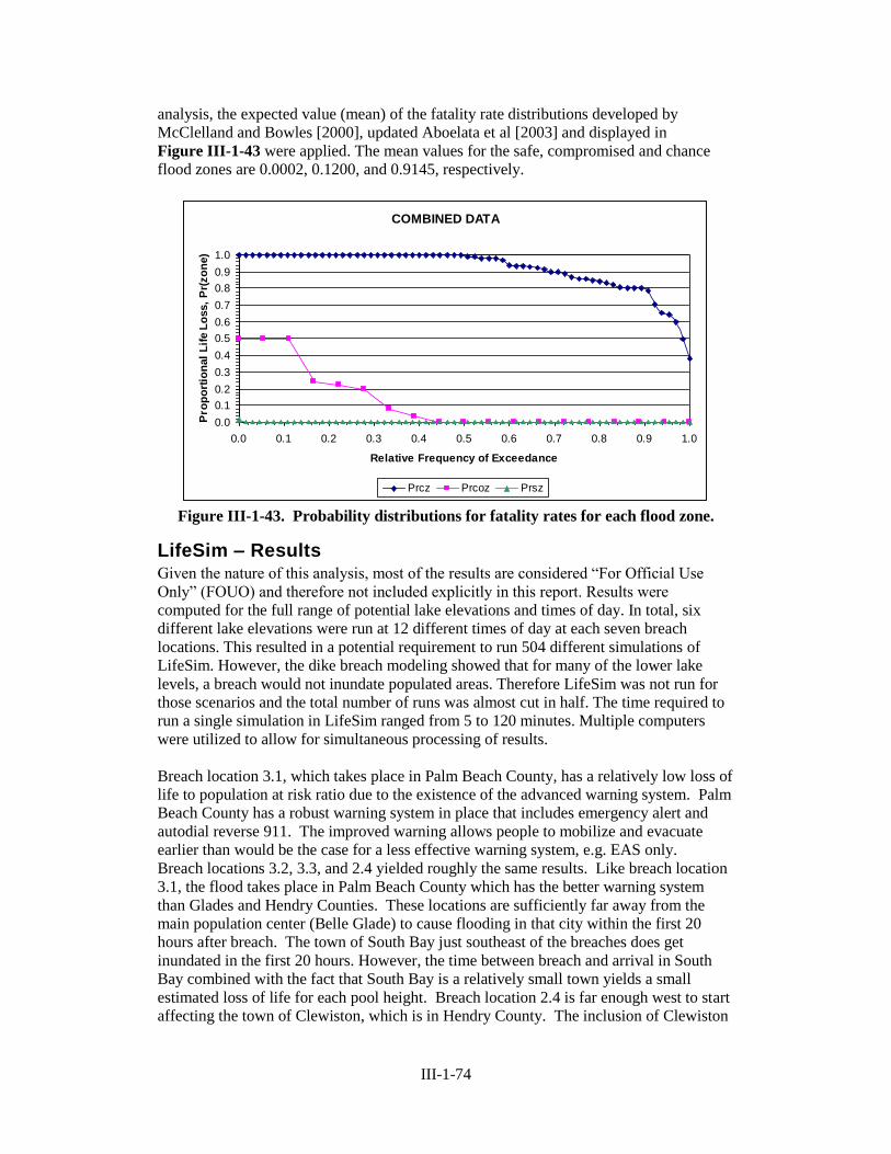
III-1-74

analysis, the expected value (mean) of the fatality rate distributions developed by

McClelland and Bowles [2000], updated Aboelata et al [2003] and displayed in

Figure III-1-43 were applied. The mean values for the safe, compromised and chance

flood zones are 0.0002, 0.1200, and 0.9145, respectively.

Figure III-1-43. Probability distributions for fatality rates for each flood zone.

LifeSim – Results Given the nature of this analysis, most of the results are considered “For Official Use

Only” (FOUO) and therefore not included explicitly in this report. Results were

computed for the full range of potential lake elevations and times of day. In total, six

different lake elevations were run at 12 different times of day at each seven breach

locations. This resulted in a potential requirement to run 504 different simulations of

LifeSim. However, the dike breach modeling showed that for many of the lower lake

levels, a breach would not inundate populated areas. Therefore LifeSim was not run for

those scenarios and the total number of runs was almost cut in half. The time required to

run a single simulation in LifeSim ranged from 5 to 120 minutes. Multiple computers

were utilized to allow for simultaneous processing of results.

Breach location 3.1, which takes place in Palm Beach County, has a relatively low loss of

life to population at risk ratio due to the existence of the advanced warning system. Palm

Beach County has a robust warning system in place that includes emergency alert and

autodial reverse 911. The improved warning allows people to mobilize and evacuate

earlier than would be the case for a less effective warning system, e.g. EAS only.

Breach locations 3.2, 3.3, and 2.4 yielded roughly the same results. Like breach location

3.1, the flood takes place in Palm Beach County which has the better warning system

than Glades and Hendry Counties. These locations are sufficiently far away from the

main population center (Belle Glade) to cause flooding in that city within the first 20

hours after breach. The town of South Bay just southeast of the breaches does get

inundated in the first 20 hours. However, the time between breach and arrival in South

Bay combined with the fact that South Bay is a relatively small town yields a small

estimated loss of life for each pool height. Breach location 2.4 is far enough west to start

affecting the town of Clewiston, which is in Hendry County. The inclusion of Clewiston

COMBINED DATA

0.0

0.1

0.2

0.3

0.4

0.5

0.6

0.7

0.8

0.9

1.0

0.0 0.1 0.2 0.3 0.4 0.5 0.6 0.7 0.8 0.9 1.0

Relative Frequency of Exceedance

Pro

po

rtio

nal

Lif

e L

oss,

Pr(

zo

ne)

Prcz Prcoz Prsz

III-1-75

for breach location reach 2.4 led to slightly higher PAR and life loss than locations 3.2

and 3.3.

As expected, breach location 2.5 has the highest estimated life loss and PAR in the study.

The breach occurs at the town of Clewiston, which is right next to the dike. The highest

life loss occurs at night. This is due to the fact that the majority of people during that

time are home asleep. Since the warning system in the area is EBS, a significant portion

of the population is not getting warned early enough to allow for safe evacuation. A

breach at reach 2 point 5 with a 30 ft. pool height at night represents the worst case

scenario for this study.

Another observation when looking at results of a breach at location 2.5 is that life loss

with no pre-evacuation (lower pool levels) stays relatively small. This indicates that if

the breach occurs at high pool levels, then the inundation event will sweep through

Clewiston quickly and not allow the PAR to mobilize. If the breach occurs at lower pool

levels, then the flood will move slowly giving people more time to evacuate.

Breach location 2.6 occurs between the towns of Clewiston and Moore Haven. Like 2.5,

the highest life loss occurs at night. Since the breach occurs between two towns, the bulk

of the flood does not reach populated areas within the first 20 hours resulting in a much

lower PAR.

Breach location 2.7 occurs at the town of Moore Haven. By nature of the flooding that

would occur at this location and the smaller size of the town in comparison to Clewiston

a far lower loss of life was estimated than reach 2.5. The town of Moore Haven has a

large canal going through it that can hold a portion of the flood as the breach occurs.

This allows the inhabitants valuable time to evacuate. Also, Moore Haven is located

farther away from the dike than Clewiston, which also lends more time to the inhabitants

to evacuate.