III Exploring The Slowdown

Macroeconomics of GrowthStructural Constraints in Indian AgricultureImpediments to Industrial GrowthServices In The Indian Growth ProcessRegional Dimension of Economic Growth in IndiaConcluding Observations

Introduction

3.1 The recent deceleration in the Indian economy has generated considerable concern withsome apprehensions about the deepening of the slowdown and delay in revival. Several factorsare attributed to the loss of growth. Infrastructural constraints, variability and shortfalls inagricultural output, erosion in the quality of public services and gaps in technology and humandevelopment are insidiously becoming binding constraints on growth. At the same time, recentdevelopments indicate some cyclicity in output behaviour with the current phase of the cyclereflecting the general deficiency in aggregate demand, the inadequate response of privateinvestment to reforms, deceleration in public investment, inventory accumulation, excesscapacity and some evidence of consumption smoothing. In the current year, indicators of realactivity, with the exception of agriculture, have underperformed in relation to the preceding year.A few positive signs are, however, visible in the improved capital flows and the steady build-upin the foreign exchange reserves. The principal policy, instruments, i.e., fiscal and monetarypolicies have been shifted into counter-cyclical mode and the stance of policies is clearly infavour of further adjustments, if necessary, to create a congenial environment for the awaitedupturn. There is also a growing recognition that the existing level of structural reforms issuccumbing to the inexorability of diminishing returns, and bolder and more intensified reformsare required in the 'difficult areas' - agriculture, labour market, bankruptcy and exit procedures,social sector and legal reforms.

3.2 The persistence of the slowdown for the second year in succession has provoked intensedebate on the underlying causes of the downturn. Although the views traverse a wide spectrum, abroad categorisation helps to place the debate in proper perspective.

3.3 There is an influential viewpoint which attributes the deceleration to forces operating ondemand such as, low aggregate demand and adverse investment climate (NCAER, 2001), thesharp deceleration in the two major components of industrial demand-exports and investment(Acharya, 2001), the contractionary features inherent in public policies pursued in the 1990s(Shetty, 2001), and specifically, anti-cyclical fiscal policies, and the inappropriate budgetarystance (Rakshit, 2000). All of the above are reflective of a demand-constrained economy(Patnaik, 2001). Within the 'demand constraint' side of the debate, there is also the view that thedeclining trend in growth is to be attributed to demand recession as well as global slowdown(Institute of Economic Growth, 2001). The impact of contemporaneous global developments hasalso been emphasised as the overwhelming reason; one view cautions the government to beready to handle the adverse consequences of continuing global slowdown (Venkitaramanan,2001), while another suggests that "the government can do very little about it" (Economic Times,

2001). The contrarian viewpoint argues that the impact of the global slowdown on the domesticoutput growth may be minimal and the current phase may be temporary (Bhalla, 2001;Bhattacharya, 2001; Rao, 2001).

3.4 The other side of the debate ascribes the slowdown to factors operating primarily onaggregate supply. The slide in the pace of growth is attributed essentially to the growth of thecommodity producing sectors— agriculture and manufacturing (Chandrasekhar, 2001). Pointingto the institutional impediments to growth, it is argued that the main reasons for the currentslowdown are structural and should be addressed accordingly (Karnik, 2001). The slowing downof growth is also regarded as reflecting the effects of various shocks, such as, the Asian financialcrisis, international oil prices, 'patchy' monsoon and natural calamities along with deeperstructural factors at work, including infrastructure constraints, regulatory constraints in industry,agriculture and trade, and high real interest rates (IMF, 2001) as well as slow pace of reforms(International Finance Corporation, 2001). The current decelerating phase is also associated withrelatively high unemployment, poor human and social development and ecological degradation(GoI, 2001). Finally, there is the view that the recent slowdown in economic activity seems toreflect a combination of both cyclical and structural factors with different weights assignable toeither, depending on the changing conditions in the growth process (Reserve Bank of India,2001).

3.5 Against the backdrop of the current deceleration, the impassioned debate generated inIndia and the diversity of views about the downturn, this Chapter undertakes an analyticalexamination of the dynamics of India's growth performance. The approach is exploratory andempirical with the objective of presenting the findings of a series of integrated analyticalexercises on various facets of the deceleration for contributing to informed public judgement andchoice. The following section deals with the macroeconomics of growth, in terms of aggregatedemand and cyclical influences thereon, factors underlying the behaviour of aggregate demandsuch as consumption, saving, investment and net exports. Sections II and III address specificstructural constraints on aggregate supply in agriculture and industry, respectively. Section IVexamines the role of services as a lever of growth. Section V profiles the regional dimensions ofthe growth process. This is followed by concluding observations.

I. MACROECONOMICS OF GROWTH

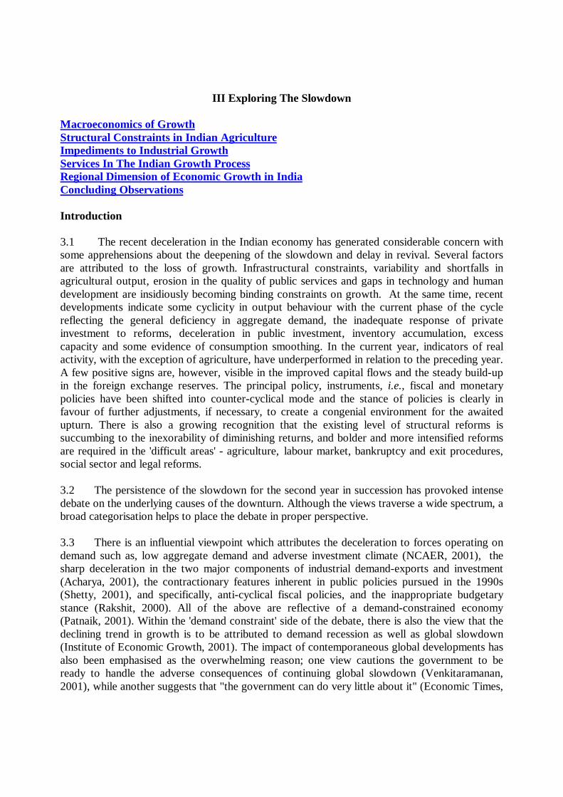
3.6 As a starting point, it is useful to date the important turning points in the time path of theIndian economy. Real GDP at factor cost represents a summary measure of economicperformance. The growth profile of real GDP in India has not been smooth and evenly paced.The Markov-switching model (Goldfeld and Quandt, 1973) can be employed to capture thedynamic patterns underlying switches or shifts in regimes which are independent over time. Thisprocedure represents an improvement over the conventional techniques that rely on priorknowledge of the existence of those shifts. The exercise reveals that the growth of GDPencountered the first 'break' in 1981-82 followed by a second 'break' in 1990-91. The first breakoccurred in the wake of the second oil shock and a severe drought. The response to these supplyshocks resulted in a step-up in the growth process with the trend growth rate rising from 3.4 percent during 1970-81 to 5.6 per cent during 1981-90. The second break is detected amidst theunprecedented balance of payments crisis associated with the Gulf war in 1990. In a similar

sequence, the simultaneous implementation of structural reform and stabilisation brought about aquantum jump in the trend growth to 6.5 per cent in the ensuing years (Chart III.1).

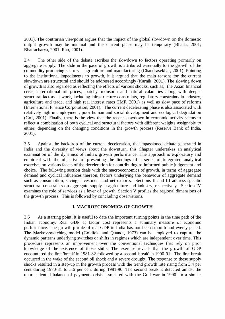
3.7 There is no evidence of a structural break in the trend growth during the 1990s whenjudged from levels; however, the growth process has also been subject to variations in pace asindicated by the recent downturn. Using the switching regression technique which employsconsecutive trial searches over the entire sample period to identify acceleration/ deceleration inreal GDP growth in terms of rates of change, an inflexion is discernible in 1978-79 showing anacceleration and again in 1995-96 with the wearing-off of the preceding high growth phases.These experiences suggest that the current phase represents a loss of speed rather than a 'break' ingrowth (Chart III.2).

3.8 Taking the diagnosis further, an incision can be made into the growth path of real GDPby decomposing it into its 'time-series' components - trend, seasonal, cyclical and irregular

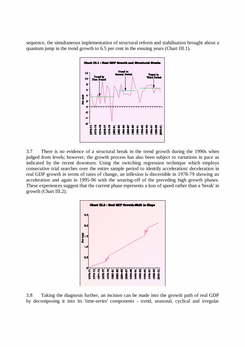
elements–depending upon the frequency and regularity of their recurrence. Seasonalcomponents are discernible in monthly and quarterly data but not in the annual data. The cyclicaland irregular components are collected together and removed by 'filtering' real GDP through thecommonly employed Hodrick-Prescott (HP) filter over the period 1970-71 to 2000-01.Separating out cyclical and irregular influences from the actual growth of real GDP yields whatcan be termed as the 'structurally constrained' growth path of the economy determined by itsproduction structure, institutional characteristics and the various impediments acting onaggregate supply. The path of structurally constrained growth has undergone a distinct upwardshift in the early 1990s as liberalisation unlocked hidden capacities and unleashed repressedproductive forces. In the following years, the impetus for growth was not sustained and thestructurally constrained path tended to slope downwards in the second half of the 1990s. Thesemovements have had a fundamental influence on the potential growth path of the Indianeconomy, i.e., the growth which is realisable with the full utilisation of productive capacities inthe economy. Empirical studies conducted in India show the sensitive nature of the estimates ofpotential growth to the choice of methodology (RBI, 1999). Applying the OECD (1995) method,the potential growth path is generated from the actual data on real GDP by obtaining a locus ofthe peak growth rates achieved in the period of study and then smoothing it with a three-yearmoving average. Movements in the potential growth are found to respond to the behaviour of thestructurally constrained growth path. The liberalisation 'hump' of the early 1990s shifts thepotential growth path upwards; again the dipping of the potential growth path appears to beassociated with the slowing down of structurally constrained growth (Chart III.3). Thus, byreleasing the structural constraints, it is possible to shift the long run growth to a highertrajectory.

3.9 The exercise also provides some insights into the characteristics of cycles in the Indianeconomy. Cyclical and irregular components (which were jointly separated by using the HPfilter) are disentangled further by using a conventional business cycle filter, i.e., the Band-Passfilter (Baxter and King, 1999) which produces a smooth cycle by eliminating the outliers overthe 'band' of frequencies. The cyclical component of real GDP is depicted in Chart III.4. Itsbehaviour suggests that during the 1970s and early 1980s, cyclical fluctuations were frequent and

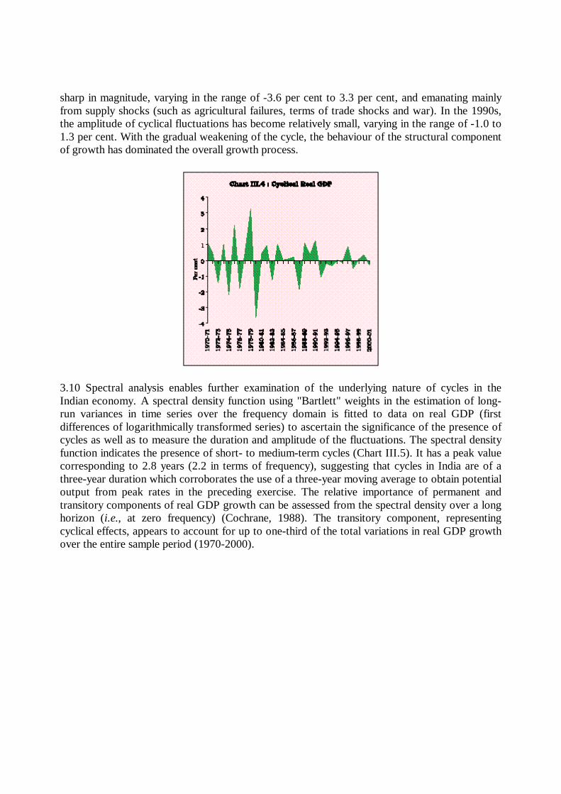
sharp in magnitude, varying in the range of -3.6 per cent to 3.3 per cent, and emanating mainlyfrom supply shocks (such as agricultural failures, terms of trade shocks and war). In the 1990s,the amplitude of cyclical fluctuations has become relatively small, varying in the range of -1.0 to1.3 per cent. With the gradual weakening of the cycle, the behaviour of the structural componentof growth has dominated the overall growth process.

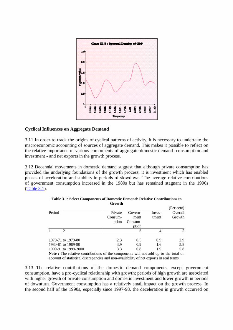
3.10 Spectral analysis enables further examination of the underlying nature of cycles in theIndian economy. A spectral density function using "Bartlett" weights in the estimation of long-run variances in time series over the frequency domain is fitted to data on real GDP (firstdifferences of logarithmically transformed series) to ascertain the significance of the presence ofcycles as well as to measure the duration and amplitude of the fluctuations. The spectral densityfunction indicates the presence of short- to medium-term cycles (Chart III.5). It has a peak valuecorresponding to 2.8 years (2.2 in terms of frequency), suggesting that cycles in India are of athree-year duration which corroborates the use of a three-year moving average to obtain potentialoutput from peak rates in the preceding exercise. The relative importance of permanent andtransitory components of real GDP growth can be assessed from the spectral density over a longhorizon (i.e., at zero frequency) (Cochrane, 1988). The transitory component, representingcyclical effects, appears to account for up to one-third of the total variations in real GDP growthover the entire sample period (1970-2000).

Cyclical Influences on Aggregate Demand

3.11 In order to track the origins of cyclical patterns of activity, it is necessary to undertake themacroeconomic accounting of sources of aggregate demand. This makes it possible to reflect onthe relative importance of various components of aggregate domestic demand -consumption andinvestment - and net exports in the growth process.

3.12 Decennial movements in domestic demand suggest that although private consumption hasprovided the underlying foundations of the growth process, it is investment which has enabledphases of acceleration and stability in periods of slowdown. The average relative contributionsof government consumption increased in the 1980s but has remained stagnant in the 1990s(Table 3.1).

Table 3.1: Select Components of Domestic Demand: Relative Contributions toGrowth

(Per cent)Period Private Govern- Inves- Overall

Consum- ment tment Growthption Consum-

ption1 2 3 4 5

1970-71 to 1979-80 2.3 0.5 0.9 2.91980-81 to 1989-90 3.9 0.9 1.6 5.81990-91 to 1999-2000 3.3 0.8 1.9 5.8Note : The relative contributions of the components will not add up to the total onaccount of statistical discrepancies and non-availability of net exports in real terms.

3.13 The relative contributions of the domestic demand components, except governmentconsumption, have a pro-cyclical relationship with growth; periods of high growth are associatedwith higher growth of private consumption and domestic investment and lower growth in periodsof downturn. Government consumption has a relatively small impact on the growth process. Inthe second half of the 1990s, especially since 1997-98, the deceleration in growth occurred on

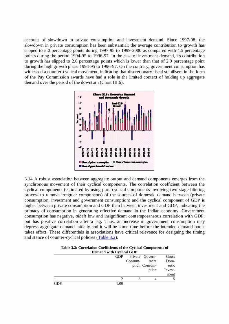
account of slowdown in private consumption and investment demand. Since 1997-98, theslowdown in private consumption has been substantial; the average contribution to growth hasslipped to 3.0 percentage points during 1997-98 to 1999-2000 as compared with 4.5 percentagepoints during the period 1994-95 to 1996-97. In the case of investment demand, its contributionto growth has slipped to 2.0 percentage points which is lower than that of 2.9 percentage pointduring the high growth phase 1994-95 to 1996-97. On the contrary, government consumption haswitnessed a counter-cyclical movement, indicating that discretionary fiscal stabilisers in the formof the Pay Commission awards have had a role in the limited context of holding up aggregatedemand over the period of the downturn (Chart III.6).

3.14 A robust association between aggregate output and demand components emerges from thesynchronous movement of their cyclical components. The correlation coefficient between thecyclical components (estimated by using pure cyclical components involving two stage filteringprocess to remove irregular components) of the sources of domestic demand between (privateconsumption, investment and government consumption) and the cyclical component of GDP ishigher between private consumption and GDP than between investment and GDP, indicating theprimacy of consumption in generating effective demand in the Indian economy. Governmentconsumption has negative, albeit low and insignificant contemporaneous correlation with GDP,but has positive correlation after a lag. Thus, an increase in government consumption maydepress aggregate demand initially and it will be some time before the intended demand boosttakes effect. These differentials in associations have critical relevance for designing the timingand stance of counter-cyclical policies (Table 3.2).

Table 3.2: Correlation Coefficients of the Cyclical Components ofDemand with Cyclical GDP

GDP Private Govern- GrossConsum- ment Dom-

ption Consum- esticption Invest-

ment1 2 3 4 5GDP 1.00

Private Consumption 0.84 1.00Government -0.08 0.17 1.00ConsumptionGross 0.34 0.02 0.20 1.00Domestic Investment

Saving Behaviour

3.15 By developing country standards, India's saving rate continues to be fairly impressive; bythe yardstick of some East-Asian economies, however, there is a considerable scope forimprovement (Table 3.3).

3.16 The Indian savings experience has been marked by varied oscillations in the saving rate(Ray and Bose, 1997). After the initial phases of low saving, it reached a high during 1976-77through 1979-80, reflecting, inter alia, the spurt in foreign remittances. Financial saving startedassuming importance as a result of the financial deepening following bank nationalisation in1969 (Table 3.4). After some lull during the first half of the 1980s reflecting deterioration inpublic savings as well as a step-up in the households' demand for consumer goods, the savingrate started recovering. The high growth phase of 1994-95 through 1996-97 is also accompaniedby a high saving phase with the average saving rate touching a high of 24.4 per cent. Theinflexion discernible in the growth rate in 1996-97 is also noticeable in the saving rates.

Table 3.3: Saving Rate in India vis-a-vis Select Asian Countries(Per cent)

Country 1990 1991 1992 1993 1994 1995 1996 1997 1998 1999 1990-99*1 2 3 4 5 6 7 8 9 10 11 12India 23.1 22.0 21.8 22.5 24.8 25.1 23.2 23.5 22.0 22.3 23.0Singapore 43.4 44.7 45.1 45.3 47.3 49.7 49.5 50.4 50.6 49.9 47.6Malaysia 34.4 34.1 36.7 39.1 39.6 39.7 42.9 43.8 48.5 47.0 40.6Hong Kong 35.4 33.8 33.8 34.6 33.1 30.5 30.7 31.1 30.2 29.9 32.3China 38.7 39.2 40.1 41.7 42.7 42.5 41.1 41.5 40.8 39.0 40.7Republic of Korea 37.2 37.2 36.3 36.0 35.4 35.6 34.0 33.7 34.2 34.2 35.4Indonesia 32.3 33.5 35.3 32.5 32.2 30.6 30.1 31.5 28.4 19.5 30.6

* Average for the period.Source : Asian Development Bank.Note : Data for India is for April-March and for others on calendar year basis.

3.17 Several factors influencing saving behaviour such as income, interest rates and othervariables have been explored in the empirical literature, using cross-section and time series data.Real GDP growth has generally been found to have exerted a positive effect on the savings rate(Fry, 1980; Giovannini, 1985). Contrary to conventional wisdom, some empirical studies havefound a negative effect of real interest rate on savings (Giovannini, 1985). The transformation ofdomestic savings into additional income via accumulation of capital was found to be not onlyoperative, but a significant factor in the growth of incomes in developing countries (Gersovitz,1988). Saving is not just about accumulation but about smoothing consumption in the presenceof liquidity constraints and uncertainties including those associated with the full stream ofincome on part of the individual households, typically in developing economies (Deaton, 1990).The issues pertaining to the effect of various determinants of savings are, thus, yet to be fullyresolved.

3.18 In the Indian context, income is identified as an important variable in explaining savingsrate, particularly for the household sector (Krishnaswamy, Krishnamurty and Sharma, 1987).Granger causality tests found evidence for growth influencing savings and not vice-versa. Otherimportant determinants of savings behaviour are found to be the size of the working population,dependency ratio, financial deepening and taxation (Mulheisen, 1997). The studies on the effectof interest rate on savings in India have showed mixed results. A disaggregated analysis on theeffect of the real interest rate on saving found a favourable impact of the rate of interest on somecomponents of savings, i.e., currency and bank deposits (Pandit, 1985), and of the real interestrate on the savings rate of the households as well as for the economy as a whole (Krishnaswamy,Krishnamurty and Sharma, 1987), whereas other studies have yielded inconclusive resultsrelating to the interest sensitivity of savings behaviour in India (Bhattacharya, 1985). Besides,spread of banking has been found to have a significant impact on savings (Krishnaswamy,Krishnamurty and Sharma, 1987).

Table 3.4: Behaviour of Aggregate and Sectoral Savings(As percentage of GDP at current market prices)

Period / Year Households Private Public Gross DomesticFinancial Physical Total Corporate Saving

1 2 3 4 5 6 7

1976-77 to 1978-79 5.7 8.5 14.3 1.4 4.6 20.21979-80 to 1984-85 6.1 7.1 13.3 1.6 3.8 18.71995-86 to 1992-93 7.9 8.9 16.7 2.3 2.1 21.11993-94 11.0 7.4 18.4 3.5 0.6 22.51994-95 11.9 7.8 19.7 3.5 1.7 24.81995-96 8.9 9.3 18.1 4.9 2.0 25.11996-97 10.3 6.7 17.0 4.5 1.7 23.21997-98 9.9 8.0 17.8 4.2 1.5 23.51998-99 10.9 8.2 19.1 3.7 -0.8 22.01999-2000 10.5 9.2 19.8 3.7 -1.2 22.3

Source : Central Statistical Organisation.

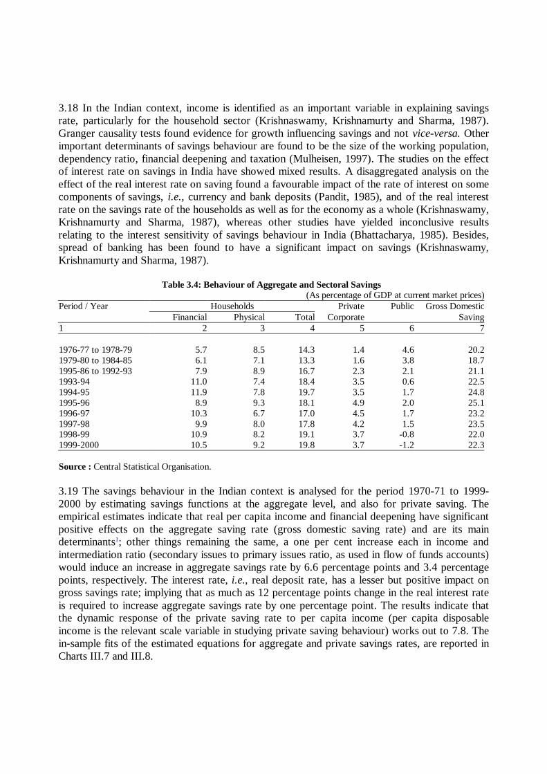
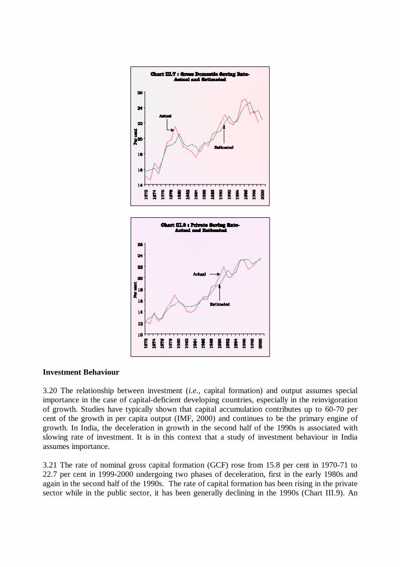
3.19 The savings behaviour in the Indian context is analysed for the period 1970-71 to 1999-2000 by estimating savings functions at the aggregate level, and also for private saving. Theempirical estimates indicate that real per capita income and financial deepening have significantpositive effects on the aggregate saving rate (gross domestic saving rate) and are its maindeterminants1; other things remaining the same, a one per cent increase each in income andintermediation ratio (secondary issues to primary issues ratio, as used in flow of funds accounts)would induce an increase in aggregate savings rate by 6.6 percentage points and 3.4 percentagepoints, respectively. The interest rate, i.e., real deposit rate, has a lesser but positive impact ongross savings rate; implying that as much as 12 percentage points change in the real interest rateis required to increase aggregate savings rate by one percentage point. The results indicate thatthe dynamic response of the private saving rate to per capita income (per capita disposableincome is the relevant scale variable in studying private saving behaviour) works out to 7.8. Thein-sample fits of the estimated equations for aggregate and private savings rates, are reported inCharts III.7 and III.8.

Investment Behaviour

3.20 The relationship between investment (i.e., capital formation) and output assumes specialimportance in the case of capital-deficient developing countries, especially in the reinvigorationof growth. Studies have typically shown that capital accumulation contributes up to 60-70 percent of the growth in per capita output (IMF, 2000) and continues to be the primary engine ofgrowth. In India, the deceleration in growth in the second half of the 1990s is associated withslowing rate of investment. It is in this context that a study of investment behaviour in Indiaassumes importance.

3.21 The rate of nominal gross capital formation (GCF) rose from 15.8 per cent in 1970-71 to22.7 per cent in 1999-2000 undergoing two phases of deceleration, first in the early 1980s andagain in the second half of the 1990s. The rate of capital formation has been rising in the privatesector while in the public sector, it has been generally declining in the 1990s (Chart III.9). An

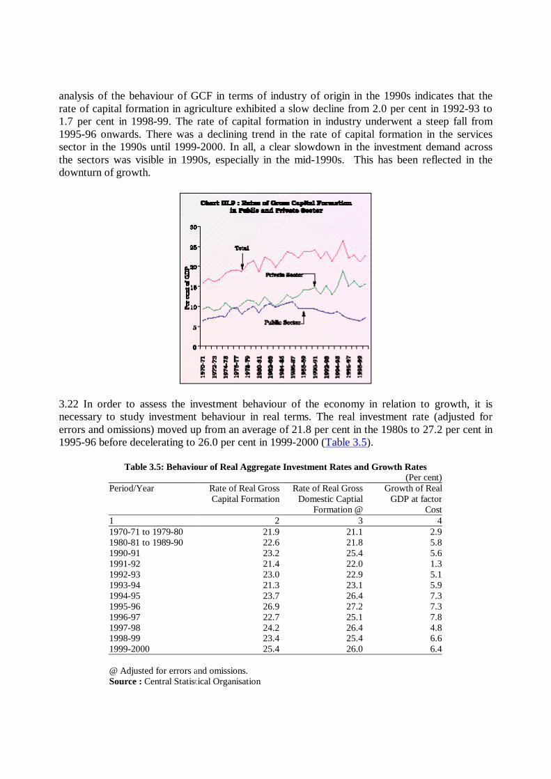
analysis of the behaviour of GCF in terms of industry of origin in the 1990s indicates that therate of capital formation in agriculture exhibited a slow decline from 2.0 per cent in 1992-93 to1.7 per cent in 1998-99. The rate of capital formation in industry underwent a steep fall from1995-96 onwards. There was a declining trend in the rate of capital formation in the servicessector in the 1990s until 1999-2000. In all, a clear slowdown in the investment demand acrossthe sectors was visible in 1990s, especially in the mid-1990s. This has been reflected in thedownturn of growth.

3.22 In order to assess the investment behaviour of the economy in relation to growth, it isnecessary to study investment behaviour in real terms. The real investment rate (adjusted forerrors and omissions) moved up from an average of 21.8 per cent in the 1980s to 27.2 per cent in1995-96 before decelerating to 26.0 per cent in 1999-2000 (Table 3.5).

Table 3.5: Behaviour of Real Aggregate Investment Rates and Growth Rates(Per cent)

Period/Year Rate of Real Gross Rate of Real Gross Growth of RealCapital Formation Domestic Captial GDP at factor

Formation @ Cost1 2 3 41970-71 to 1979-80 21.9 21.1 2.91980-81 to 1989-90 22.6 21.8 5.81990-91 23.2 25.4 5.61991-92 21.4 22.0 1.31992-93 23.0 22.9 5.11993-94 21.3 23.1 5.91994-95 23.7 26.4 7.31995-96 26.9 27.2 7.31996-97 22.7 25.1 7.81997-98 24.2 26.4 4.81998-99 23.4 25.4 6.61999-2000 25.4 26.0 6.4

@ Adjusted for errors and omissions.Source : Central Statistical Organisation

3.23 The traditional view of investment in the context of growth cycles is in terms of itsreplacement cost. In a developing economy, apart from the rate of output growth, andreplacement cost (or cost of capital), the rate of capacity utilisation, liquidity constraints faced byfirms, and macroeconomic stability have been identified as major determinants of investment(Schimidt-Hebbel, Seren, and Solmano, 1996). An important issue in the study of investment inIndia is the relation between public and private investment, particularly in the context of thevacation of public investment in several areas to create space for private investment as part of thestructural reforms in the 1990s. In India, the broad consensus favours a crowding-in relationshipbetween public and private investment (Sundarajan and Thakur, 1980). The major determinantsof corporate investment in India have been found to be credit availability and cost of capital(Athukorala and Sen, 1996).

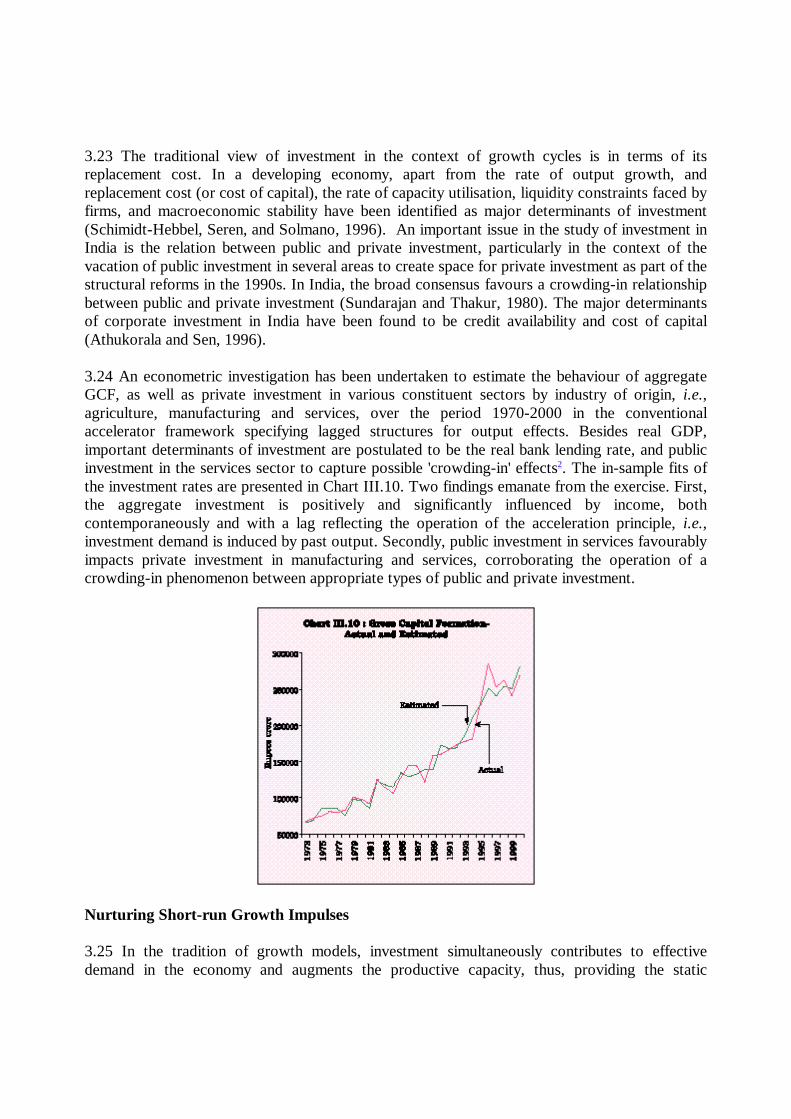
3.24 An econometric investigation has been undertaken to estimate the behaviour of aggregateGCF, as well as private investment in various constituent sectors by industry of origin, i.e.,agriculture, manufacturing and services, over the period 1970-2000 in the conventionalaccelerator framework specifying lagged structures for output effects. Besides real GDP,important determinants of investment are postulated to be the real bank lending rate, and publicinvestment in the services sector to capture possible 'crowding-in' effects2. The in-sample fits ofthe investment rates are presented in Chart III.10. Two findings emanate from the exercise. First,the aggregate investment is positively and significantly influenced by income, bothcontemporaneously and with a lag reflecting the operation of the acceleration principle, i.e.,investment demand is induced by past output. Secondly, public investment in services favourablyimpacts private investment in manufacturing and services, corroborating the operation of acrowding-in phenomenon between appropriate types of public and private investment.

Nurturing Short-run Growth Impulses

3.25 In the tradition of growth models, investment simultaneously contributes to effectivedemand in the economy and augments the productive capacity, thus, providing the static

Keynesian analysis with a dynamic perspective. In this section, the analysis hopes to providepointers for the allocation of resources in support of reviving growth. For this purpose, workingout investment multipliers and accelerators as well as multiplier-accelerator interaction becomescrucial for gauging the strength and duration of virtuous cycles of investment and output so as todirect the deployment of investible resources. The multiplier determines the initial injection ofinvestment that is necessary to generate a desired increase in income. The accelerator measuresthe response of investment to changes in demand conditions. The multiplier and acceleratortogether capture the simultaneous interaction of investment and income (demand).

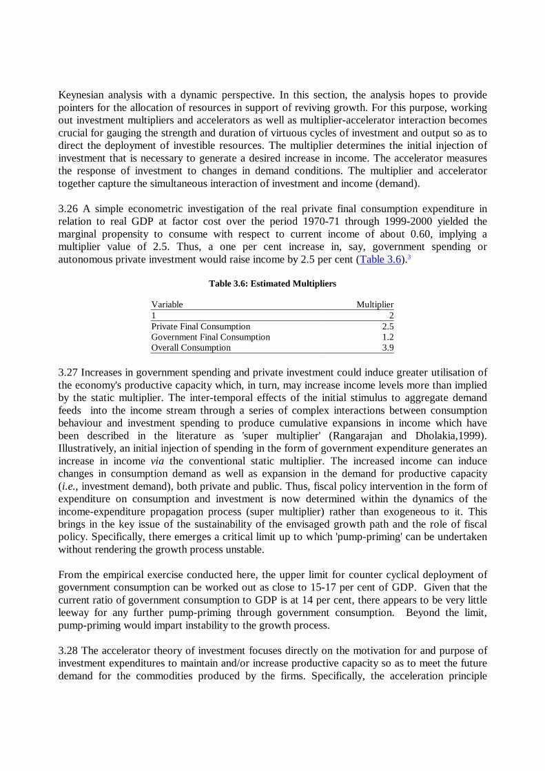
3.26 A simple econometric investigation of the real private final consumption expenditure inrelation to real GDP at factor cost over the period 1970-71 through 1999-2000 yielded themarginal propensity to consume with respect to current income of about 0.60, implying amultiplier value of 2.5. Thus, a one per cent increase in, say, government spending orautonomous private investment would raise income by 2.5 per cent (Table 3.6).3

Table 3.6: Estimated Multipliers

Variable Multiplier1 2Private Final Consumption 2.5Government Final Consumption 1.2Overall Consumption 3.9

3.27 Increases in government spending and private investment could induce greater utilisation ofthe economy's productive capacity which, in turn, may increase income levels more than impliedby the static multiplier. The inter-temporal effects of the initial stimulus to aggregate demandfeeds into the income stream through a series of complex interactions between consumptionbehaviour and investment spending to produce cumulative expansions in income which havebeen described in the literature as 'super multiplier' (Rangarajan and Dholakia,1999).Illustratively, an initial injection of spending in the form of government expenditure generates anincrease in income via the conventional static multiplier. The increased income can inducechanges in consumption demand as well as expansion in the demand for productive capacity(i.e., investment demand), both private and public. Thus, fiscal policy intervention in the form ofexpenditure on consumption and investment is now determined within the dynamics of theincome-expenditure propagation process (super multiplier) rather than exogeneous to it. Thisbrings in the key issue of the sustainability of the envisaged growth path and the role of fiscalpolicy. Specifically, there emerges a critical limit up to which 'pump-priming' can be undertakenwithout rendering the growth process unstable.

From the empirical exercise conducted here, the upper limit for counter cyclical deployment ofgovernment consumption can be worked out as close to 15-17 per cent of GDP. Given that thecurrent ratio of government consumption to GDP is at 14 per cent, there appears to be very littleleeway for any further pump-priming through government consumption. Beyond the limit,pump-priming would impart instability to the growth process.

3.28 The accelerator theory of investment focuses directly on the motivation for and purpose ofinvestment expenditures to maintain and/or increase productive capacity so as to meet the futuredemand for the commodities produced by the firms. Specifically, the acceleration principle

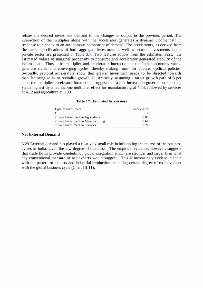
relates the desired investment demand to the changes in output in the previous period. Theinteraction of the multiplier along with the accelerator generates a dynamic income path inresponse to a shock to an autonomous component of demand. The accelerators, as derived fromthe earlier specifications of both aggregate investment as well as sectoral investments in theprivate sector are presented in Table 3.7. Two features follow from the estimates. First, theestimated values of marginal propensity to consume and accelerator generated stability of theincome path. Thus, the multiplier and accelerator interaction in the Indian economy wouldgenerate stable and converging cycles, thereby making room for counter cyclical policies.Secondly, sectoral accelerators show that greater investment needs to be directed towardsmanufacturing so as to revitalise growth. Illustratively, assuming a target growth path of 8 percent, the multiplier-accelerator interactions suggest that a unit increase in government spendingyields highest dynamic income multiplier effect for manufacturing at 4.73, followed by servicesat 4.12 and agriculture at 3.89.

Table 3.7 : Estimated Accelerators

Type of Investment Accelerator1 2Private Investment in Agriculture 0.04Private Investment in Manufacturing 0.61Private Investment in Services 0.21

Net External Demand

3.29 External demand has played a relatively small role in influencing the course of the businesscycles in India, given the low degree of openness. The empirical evidence, however, suggeststhat trade flows provide conduits for global integration which are stronger and larger than whatany conventional measure of net exports would suggest. This is increasingly evident in Indiawith the pattern of exports and industrial production exhibiting certain degree of co-movementwith the global business cycle (Chart III.11).

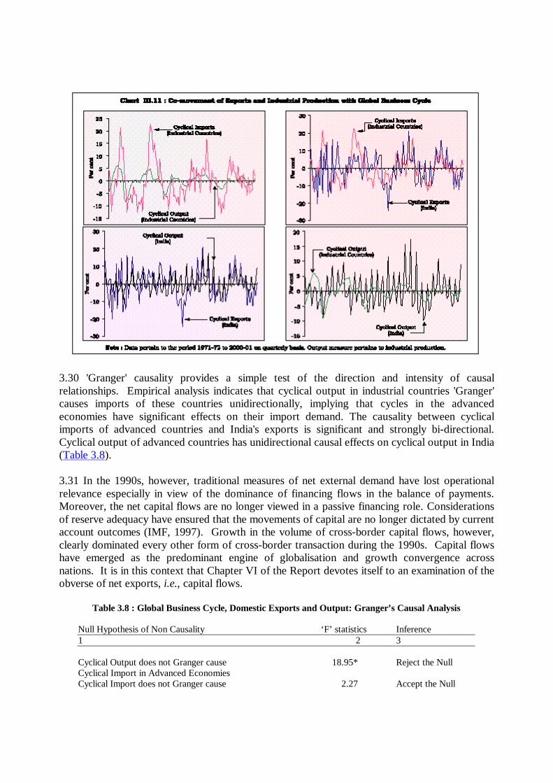
3.30 'Granger' causality provides a simple test of the direction and intensity of causalrelationships. Empirical analysis indicates that cyclical output in industrial countries 'Granger'causes imports of these countries unidirectionally, implying that cycles in the advancedeconomies have significant effects on their import demand. The causality between cyclicalimports of advanced countries and India's exports is significant and strongly bi-directional.Cyclical output of advanced countries has unidirectional causal effects on cyclical output in India(Table 3.8).

3.31 In the 1990s, however, traditional measures of net external demand have lost operationalrelevance especially in view of the dominance of financing flows in the balance of payments.Moreover, the net capital flows are no longer viewed in a passive financing role. Considerationsof reserve adequacy have ensured that the movements of capital are no longer dictated by currentaccount outcomes (IMF, 1997). Growth in the volume of cross-border capital flows, however,clearly dominated every other form of cross-border transaction during the 1990s. Capital flowshave emerged as the predominant engine of globalisation and growth convergence acrossnations. It is in this context that Chapter VI of the Report devotes itself to an examination of theobverse of net exports, i.e., capital flows.

Table 3.8 : Global Business Cycle, Domestic Exports and Output: Granger’s Causal Analysis

Null Hypothesis of Non Causality ‘F’ statistics Inference1 2 3

Cyclical Output does not Granger cause 18.95* Reject the NullCyclical Import in Advanced EconomiesCyclical Import does not Granger cause 2.27 Accept the Null

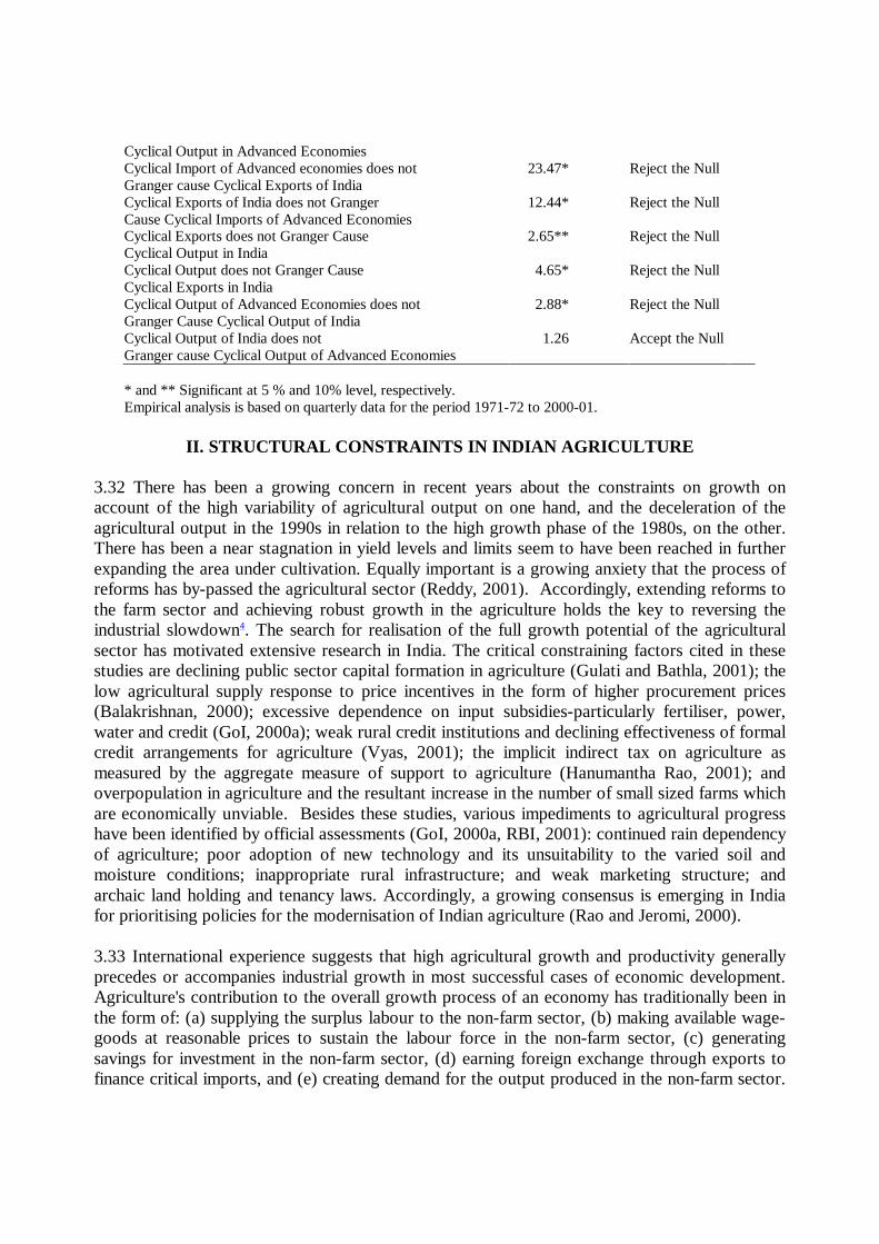
Cyclical Output in Advanced EconomiesCyclical Import of Advanced economies does not 23.47* Reject the NullGranger cause Cyclical Exports of IndiaCyclical Exports of India does not Granger 12.44* Reject the NullCause Cyclical Imports of Advanced EconomiesCyclical Exports does not Granger Cause 2.65** Reject the NullCyclical Output in IndiaCyclical Output does not Granger Cause 4.65* Reject the NullCyclical Exports in IndiaCyclical Output of Advanced Economies does not 2.88* Reject the NullGranger Cause Cyclical Output of IndiaCyclical Output of India does not 1.26 Accept the NullGranger cause Cyclical Output of Advanced Economies

* and ** Significant at 5 % and 10% level, respectively.Empirical analysis is based on quarterly data for the period 1971-72 to 2000-01.

II. STRUCTURAL CONSTRAINTS IN INDIAN AGRICULTURE

3.32 There has been a growing concern in recent years about the constraints on growth onaccount of the high variability of agricultural output on one hand, and the deceleration of theagricultural output in the 1990s in relation to the high growth phase of the 1980s, on the other.There has been a near stagnation in yield levels and limits seem to have been reached in furtherexpanding the area under cultivation. Equally important is a growing anxiety that the process ofreforms has by-passed the agricultural sector (Reddy, 2001). Accordingly, extending reforms tothe farm sector and achieving robust growth in the agriculture holds the key to reversing theindustrial slowdown4. The search for realisation of the full growth potential of the agriculturalsector has motivated extensive research in India. The critical constraining factors cited in thesestudies are declining public sector capital formation in agriculture (Gulati and Bathla, 2001); thelow agricultural supply response to price incentives in the form of higher procurement prices(Balakrishnan, 2000); excessive dependence on input subsidies-particularly fertiliser, power,water and credit (GoI, 2000a); weak rural credit institutions and declining effectiveness of formalcredit arrangements for agriculture (Vyas, 2001); the implicit indirect tax on agriculture asmeasured by the aggregate measure of support to agriculture (Hanumantha Rao, 2001); andoverpopulation in agriculture and the resultant increase in the number of small sized farms whichare economically unviable. Besides these studies, various impediments to agricultural progresshave been identified by official assessments (GoI, 2000a, RBI, 2001): continued rain dependencyof agriculture; poor adoption of new technology and its unsuitability to the varied soil andmoisture conditions; inappropriate rural infrastructure; and weak marketing structure; andarchaic land holding and tenancy laws. Accordingly, a growing consensus is emerging in Indiafor prioritising policies for the modernisation of Indian agriculture (Rao and Jeromi, 2000).

3.33 International experience suggests that high agricultural growth and productivity generallyprecedes or accompanies industrial growth in most successful cases of economic development.Agriculture's contribution to the overall growth process of an economy has traditionally been inthe form of: (a) supplying the surplus labour to the non-farm sector, (b) making available wage-goods at reasonable prices to sustain the labour force in the non-farm sector, (c) generatingsavings for investment in the non-farm sector, (d) earning foreign exchange through exports tofinance critical imports, and (e) creating demand for the output produced in the non-farm sector.

The changing mix and the continuous interaction between the farm and the non-farm sectorassumes critical importance in the growth process as it offers opportunities for internalising thesynergetic growth impulses even in a period of decline in the share of agriculture in real GDP.

3.34 In India, agriculture occupies a special position in the development process. It continues toprovide a ratchet to the overall GDP growth, in view of the continued dependence of up to two-thirds of the population on agriculture. In this section, an attempt is made to identify theconstraints to higher agricultural growth. Drawing from an overview of the changing pattern ofgrowth and productivity of Indian agriculture over the past three decades, an analysis of themajor determinants of agricultural growth in India is undertaken to identify bottlenecks chokingthe growth prospects of Indian agriculture and to suggest proximate solutions.

Changing Patterns of Growth and Productivity

3.35 Agricultural output growth registered a sharp increase in the immediate post-greenrevolution phase largely due to a growth in yields; however, the growth pattern has not beenuniform with a tendency towards deceleration in the 1990s (Table 3.9 and Charts III.12 andIII.13).

Table 3.9: Trend Growth Rates in the Indices of Area, Production and Yields of Foodgrains, Non-Foodgrains and All Crops during 1970-71 to 2000-01

(per cent)Period Foodgrains Non-Foodgrains All Crops

Area Production Yield Area Production Yield Area Production Yield1 2 3 4 5 6 7 8 9 10

1970-71 to -0.03 2.52 2.13 1.46 3.31 1.66 0.35 2.83 1.932000-01

1970-71 to 0.44 1.91 1.06 1.10 2.15 1.00 0.59 1.99 1.031979-80

1980-81 to -0.22 2.81 2.71 1.11 3.70 2.28 0.09 3.13 2.521989-90

1990-91 to 0.07 1.98 1.30 1.29 2.77 1.08 0.41 2.30 1.191999-2000

Note : Trend Growth Rates are based on semi-logarithmic function.

3.36 The yield pattern in case of both foodgrains and non-foodgrains indicates that highestgrowth in yield levels occurred during the 1980s. Much of the growth in agricultural productionin India is yield-driven as the growth in area is marginal; however, Indian agriculture suffersfrom lower yield levels vis-à-vis major agricultural producers in the world, despite India beingone of the largest producers of most of the major crops (Table 3.10). The yield of 6,059 kg perhectare attained in China during 1998 in the production of paddy was more than double that of2,890 kg per hectare in India. Similarly, wheat yield in China stood at 3,667 kg per hectare in1998 in comparison with 2,578 kg per hectare in India.

Table 3.10 : India’s Global Rank in Major Agricultural Crops

Crop Rank in 2000Area Production Yield

1 2 3 4

Rice (Paddy) 1 2 52Wheat 1 2 38Coarse Grains 3 4 125Pulses 1 1 138Oil Crops (Primary) 2 5 147Cotton Seed 1 4 77Jute and Jute Like Fibres 1 1 7Tea 2 1 13Coffee (Green) 7 7 14Sugarcane 2 2 31

Source : Food and Agricultural Organisation.

The Role of Technology in Indian Agriculture

3.37 One of the main reasons for the low levels of yield attained in India is the unsatisfactoryspread of new technological practices, including cultivation of High Yielding Varieties (HYV) ofseeds. The adoption of new technology, mainly the cultivation of HYV seeds requires intensiveuse of fertilisers and pesticides under adequate and often assured water supply. The use of HYVseeds entails a higher yield risk (as measured by variance in yield) as compared with thetraditional seed varieties, in the absence of proper irrigation facilities (Ganesh Kumar, 1999;Saha, 2001). The lower spread of new technological practices to a wide variety of crops otherthan wheat and rice as also across regions could be attributed to the higher yield risk associatedwith the cultivation of HYV seeds, caused by inadequate spread of irrigation facilities. There isconsiderable co-movement between the area under HYV seeds and area under irrigation,probably on account of reduction in yield risk due to irrigation facilities (Chart III.14).

3.38 It is mainly paddy and wheat, which are cultivated under the HYV seeds, while the areasunder HYV seeds for other cereal crops are very low and vary across different States of thecountry. Low growth experienced during the past two decades in the production of coarsecereals (0.5 per cent) and pulses (0.8 per cent) in comparison to rice (2.8 per cent) and wheat (4.0per cent) is on account of lower adoption of HYV seeds or non-availability of appropriate seeds

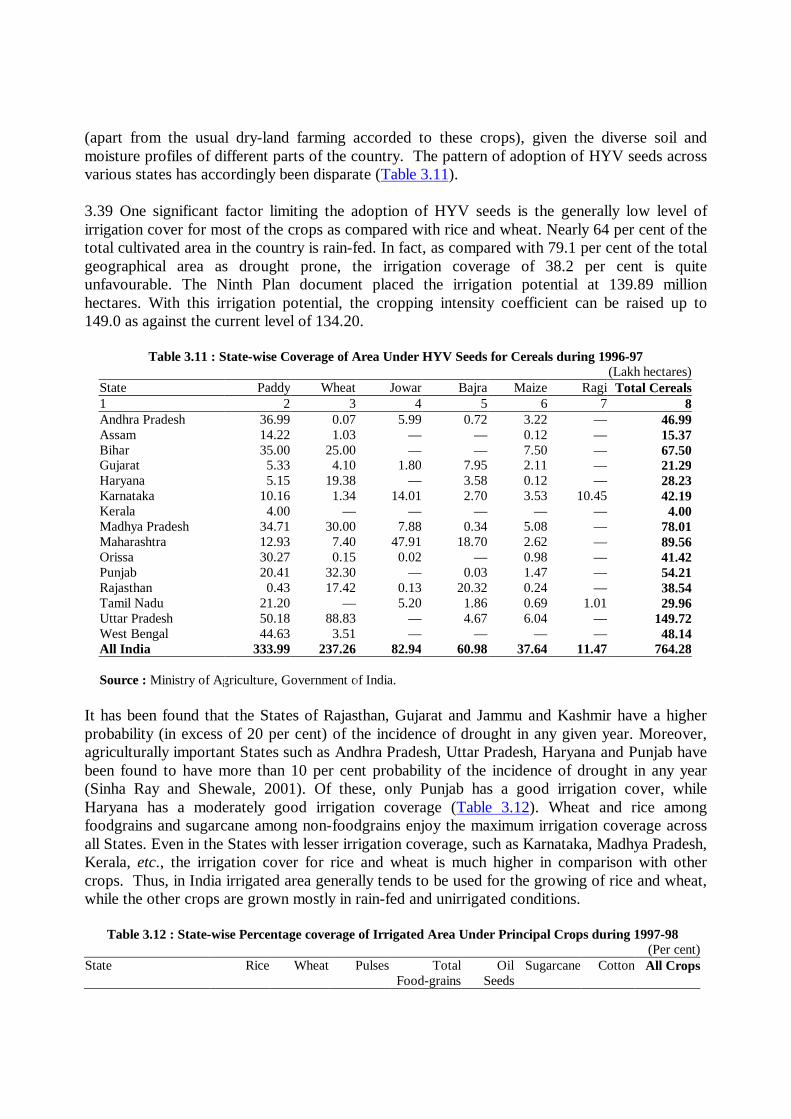
(apart from the usual dry-land farming accorded to these crops), given the diverse soil andmoisture profiles of different parts of the country. The pattern of adoption of HYV seeds acrossvarious states has accordingly been disparate (Table 3.11).

3.39 One significant factor limiting the adoption of HYV seeds is the generally low level ofirrigation cover for most of the crops as compared with rice and wheat. Nearly 64 per cent of thetotal cultivated area in the country is rain-fed. In fact, as compared with 79.1 per cent of the totalgeographical area as drought prone, the irrigation coverage of 38.2 per cent is quiteunfavourable. The Ninth Plan document placed the irrigation potential at 139.89 millionhectares. With this irrigation potential, the cropping intensity coefficient can be raised up to149.0 as against the current level of 134.20.

Table 3.11 : State-wise Coverage of Area Under HYV Seeds for Cereals during 1996-97(Lakh hectares)

State Paddy Wheat Jowar Bajra Maize Ragi Total Cereals1 2 3 4 5 6 7 8Andhra Pradesh 36.99 0.07 5.99 0.72 3.22 — 46.99Assam 14.22 1.03 — — 0.12 — 15.37Bihar 35.00 25.00 — — 7.50 — 67.50Gujarat 5.33 4.10 1.80 7.95 2.11 — 21.29Haryana 5.15 19.38 — 3.58 0.12 — 28.23Karnataka 10.16 1.34 14.01 2.70 3.53 10.45 42.19Kerala 4.00 — — — — — 4.00Madhya Pradesh 34.71 30.00 7.88 0.34 5.08 — 78.01Maharashtra 12.93 7.40 47.91 18.70 2.62 — 89.56Orissa 30.27 0.15 0.02 — 0.98 — 41.42Punjab 20.41 32.30 — 0.03 1.47 — 54.21Rajasthan 0.43 17.42 0.13 20.32 0.24 — 38.54Tamil Nadu 21.20 — 5.20 1.86 0.69 1.01 29.96Uttar Pradesh 50.18 88.83 — 4.67 6.04 — 149.72West Bengal 44.63 3.51 — — — — 48.14All India 333.99 237.26 82.94 60.98 37.64 11.47 764.28

Source : Ministry of Agriculture, Government of India.

It has been found that the States of Rajasthan, Gujarat and Jammu and Kashmir have a higherprobability (in excess of 20 per cent) of the incidence of drought in any given year. Moreover,agriculturally important States such as Andhra Pradesh, Uttar Pradesh, Haryana and Punjab havebeen found to have more than 10 per cent probability of the incidence of drought in any year(Sinha Ray and Shewale, 2001). Of these, only Punjab has a good irrigation cover, whileHaryana has a moderately good irrigation coverage (Table 3.12). Wheat and rice amongfoodgrains and sugarcane among non-foodgrains enjoy the maximum irrigation coverage acrossall States. Even in the States with lesser irrigation coverage, such as Karnataka, Madhya Pradesh,Kerala, etc., the irrigation cover for rice and wheat is much higher in comparison with othercrops. Thus, in India irrigated area generally tends to be used for the growing of rice and wheat,while the other crops are grown mostly in rain-fed and unirrigated conditions.

Table 3.12 : State-wise Percentage coverage of Irrigated Area Under Principal Crops during 1997-98(Per cent)

State Rice Wheat Pulses Total Oil Sugarcane Cotton All CropsFood-grains Seeds

1 2 3 4 5 6 7 8 9Andhra Pradesh 96.4 72.7 1.2 55.1 19.7 95.2 18.9 42.5Bihar 40.4 89.0 2.1 47.8 20.2 30.6 — 46.6Gujarat 61.2 75.6 10.7 32.2 26.0 100.0 37.7 34.3Haryana 99.6 98.3 22.5 77.5 70.0 97.9 98.9 78.6Karnataka 69.2 38.2 3.9 22.5 21.3 100.0 19.3 24.9Kerala 52.2 — — 49.3 16.0 100.0 — 14.0Madhya Pradesh 23.6 69.2 18.5 30.4 5.7 98.6 39.4 25.0Maharashtra 28.1 69.6 7.3 13.3 11.1 95.0 2.8 14.5Orissa 36.2 100.0 5.0 26.7 11.0 100.0 — 26.8Punjab 95.0 94.8 89.8 93.8 62.2 75.1 99.6 91.7Rajasthan 41.5 94.7 7.7 23.6 43.9 100.0 98.0 29.9Tamil Nadu 93.2 — 6.4 62.0 40.9 100.0 34.6 53.7Uttar Pradesh 62.7 91.7 27.7 64.7 39.5 95.0 91.7 65.9West Bengal 25.9 73.0 4.5 27.6 63.5 30.8 — 27.1All India 50.2 85.0 11.8 40.6 24.4 92.6 36.3 38.2

Source : Ministry of Agriculture, Government of India.

3.40 In such a scenario, the technological development in terms of the adoption of HYV seeds ismostly limited to the cultivation of rice and wheat on account of higher yield risk imparted bythese seeds. It is pertinent to note in this connection that the foodgrains production in 1999-2000was at a record high of 208.9 million tonnes despite acute drought conditions in the centralstretch of India, mainly on account of record production of rice and wheat. Most of the othercrops - mainly oilseeds - suffered significant fall in production in that year. This could beindicative of the disproportionate adoption of technology and irrigation benefits, underscoringthe need for spreading the irrigation benefits to all crops.

3.41 Another important factor affecting the dissemination of modern technology in general andHYV seed technology in particular is the small size of average farms in India. It has been arguedthat the small size of land holdings limits the adoption of new technology due to reasons otherthan the scale of operation. Share-cropping, which is generally undertaken by the small andmarginal farmers, limits the scope for adoption of new technology as the farmer has to pay afraction of (generally around half) the production to the land-owner, while the whole cost ofadoption of the green revolution inputs such as HYV seeds and fertilisers will have to be borneby the tenant. In such an arrangement, it is imperative that the gains in marginal product due toadoption of these inputs should at least be twice that of the investment for the farmer to breakeven. Such dramatic increases in production are difficult to come by in the absence of otherinfrastructural facilities and hence, the scope for adoption of green revolution inputs by theshare-cropper is clearly undermined.

3.42 The per hectare consumption of fertilisers and pesticides is quite low in India in comparisonwith international standards and there is a lot of scope for improvement in this sphere. Forinstance, the per hectare consumption of fertilisers in India at 88.6 kg was much lower than256.6 kg and 110.4 kg in China and USA, respectively, in 1997-98. The growth in theconsumption of fertilisers during the past two decades has also quite varied across differentStates (Table 3.13). Another factor that is responsible for lower productivity of Indian agricultureis the skewed distribution of N:P:K (Nitrogen : Phosphorus : Potassium) fertiliser mix. Currently,the N:P:K ratio stands at 6.9:2.9:1.0, which is quite skewed in comparison to the optimal mix of

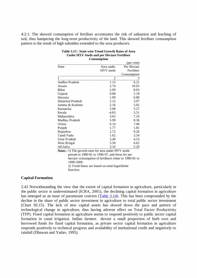
4:2:1. The skewed consumption of fertiliser accentuates the risk of salination and leaching ofsoil, thus hampering the long-term productivity of the land. This skewed fertiliser consumptionpattern is the result of high subsidies extended to the urea producers.

Table 3.13 : State-wise Trend Growth Rates of AreaUnder HYV Seeds and per Hectare Fertiliser

Consumption(per cent)

State Area under Per HectareHYV seeds Fertiliser

Consumption1 2 3Andhra Pradesh 1.15 6.21Assam 2.74 10.63Bihar 2.09 8.03Gujarat 0.68 5.18Haryana 1.09 6.80Himachal Pradesh 2.12 3.97Jammu & Kashmir 2.16 5.02Karnataka 5.68 5.27Kerala -4.83 3.51Maharashtra 3.63 7.10Madhya Pradesh 5.99 8.36Orissa 6.14 7.40Punjab 1.77 1.81Rajasthan 2.72 9.26Tamil Nadu 1.62 3.54Uttar Pradesh 3.40 4.53West Bengal 5.50 6.62All-India 3.10 5.29Notes : 1) The growth rates for area under HYV seeds

pertain to 1980-81 to 1996-97, and those for perhectare consumption of fertilisers relate to 1980-81 to1999-2000.2) Trend Rates are based on semi-logarithmicfunction.

Capital Formation

3.43 Notwithstanding the view that the extent of capital formation in agriculture, particularly inthe public sector is underestimated (ICRA, 2001), the declining capital formation in agriculturehas emerged as an issue of paramount concern (Table 3.14). This has been compounded by thedecline in the share of public sector investment in agriculture to total public sector investment(Chart III.15). The lack of new capital assets has slowed down the pace and pattern oftechnological change in agriculture, thus having adverse effect on Total Factor Productivity(TFP). Fixed capital formation in agriculture seems to respond positively to public sector capitalformation in canal irrigation. Indian farmers devote a small proportion of both own andborrowed funds for fixed capital formation, as private sector capital formation in agricultureresponds positively to technical progress and availability of institutional credit and negatively torainfall (Dhawan and Yadav, 1995).

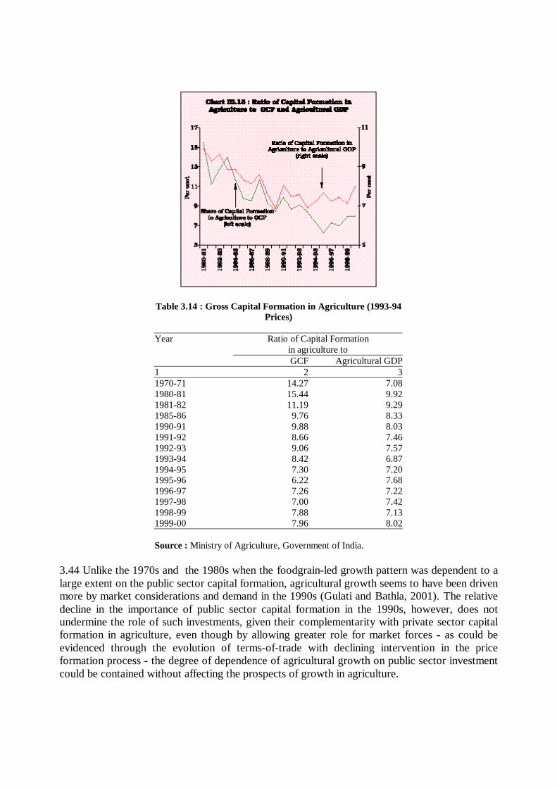
Table 3.14 : Gross Capital Formation in Agriculture (1993-94Prices)

Year Ratio of Capital Formationin agriculture toGCF Agricultural GDP

1 2 31970-71 14.27 7.081980-81 15.44 9.921981-82 11.19 9.291985-86 9.76 8.331990-91 9.88 8.031991-92 8.66 7.461992-93 9.06 7.571993-94 8.42 6.871994-95 7.30 7.201995-96 6.22 7.681996-97 7.26 7.221997-98 7.00 7.421998-99 7.88 7.131999-00 7.96 8.02

Source : Ministry of Agriculture, Government of India.

3.44 Unlike the 1970s and the 1980s when the foodgrain-led growth pattern was dependent to alarge extent on the public sector capital formation, agricultural growth seems to have been drivenmore by market considerations and demand in the 1990s (Gulati and Bathla, 2001). The relativedecline in the importance of public sector capital formation in the 1990s, however, does notundermine the role of such investments, given their complementarity with private sector capitalformation in agriculture, even though by allowing greater role for market forces - as could beevidenced through the evolution of terms-of-trade with declining intervention in the priceformation process - the degree of dependence of agricultural growth on public sector investmentcould be contained without affecting the prospects of growth in agriculture.

Storage, Processing and Marketing

3.45 The lack of proper storage and marketing facilities at the village level results in distresssales, particularly by the small and marginal farmers which adversely affect their incomes. Thishas a direct bearing on their ability to invest in agriculture. Indian agricultural marketingscenario is characterised by the existence of segmented markets on the one hand and inter-linkedmarkets on the other (Reddy, 2001). There is a geographical market segmentation characterisedby lack of market access to farmers, while there are inter-linkages in factor and product markets,which lead to lower and exploitative prices. It has been argued that the interlinked markets resultin a suboptimal situation by denying the producer an economic and market determined price forhis product (Gangopadhyay, 1994). The inter-linkage between factor and product marketscontributes significantly towards limiting the adoption of new technological inputs by way ofreducing the farmer's income. Similarly, the inter-linkages in the factor markets (for instance,between credit and labour markets) limits the technology adoption by the small farmers, by wayof putting extra-economic demand on farmer's labour at the crucial time, say sowing: thus itcontributes to lower production and hence lower income of the small farmers5.

3.46 Other important factors adversely affecting the efficiency of agricultural markets are thelack of proper futures markets, the absence of price discovery and the failure of the market inproviding proper price signals. In the absence of proper price signals, the farmers' decision tocultivate any crop may depend on less efficient criteria such as administered prices, rather thandemand and supply, leading obviously to inefficient resource allocation. Further, the existence ofa large section of unregulated middlemen and traders reduces the market efficiency to asignificant level. Bringing these middlemen into the framework of institutional marketmechanism with proper regulatory ambit will result in transforming the middlemen into marketfacilitators, while direct marketing (by producers) provides an opportunity to minimise the roleof middlemen (Reddy, 2001).

Agricultural Credit

3.47 Institutional credit to small and marginal farmers plays an important role in replacinginformal credit market mechanisms and the inter-linkages arising between informal credit andother factor/product markets. The deceleration in the growth of loans outstanding for the smallland holdings during the 1990s as compared with the 1980s is indicative of a combination ofbetter repayment of loans in the 1990s (since most of these loans are of small values and in thenature of crop loans, etc.) as well as low disbursement rate. For small and marginal farmers, thedeceleration in the credit disbursal has been the maximum in the 1990s. Small and marginalfarmers, thus, continue to be both credit and demand constrained.

3.48 The lack of capital has been a primary factor impeding the adoption of new technologicalinputs, which are capital intensive. The size and flow of financial resources to agriculture, bothin terms of investment and working capital have shrunk significantly. Despite the stipulation ofsub-targets for agriculture at 18 per cent under priority sector, credit has not flowed to thedesired extent. There exist many escape routes with regard to priority sector lending targets, suchas the option to invest in RIDF and place deposits with SIDBI. Direct finance to small andmarginal farmers (with land holdings up to two hectares) has been slowing down in recent years

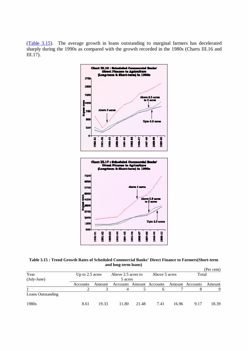
(Table 3.15). The average growth in loans outstanding to marginal farmers has deceleratedsharply during the 1990s as compared with the growth recorded in the 1980s (Charts III.16 andIII.17).

Table 3.15 : Trend Growth Rates of Scheduled Commercial Banks’ Direct Finance to Farmers(Short-termand long-term loans)

(Per cent)Year Up to 2.5 acres Above 2.5 acres to Above 5 acres Total(July-June) 5 acres

Accounts Amount Accounts Amount Accounts Amount Accounts Amount1 2 3 4 5 6 7 8 9Loans Outstanding

1980s 8.61 19.33 11.80 21.48 7.41 16.96 9.17 18.39

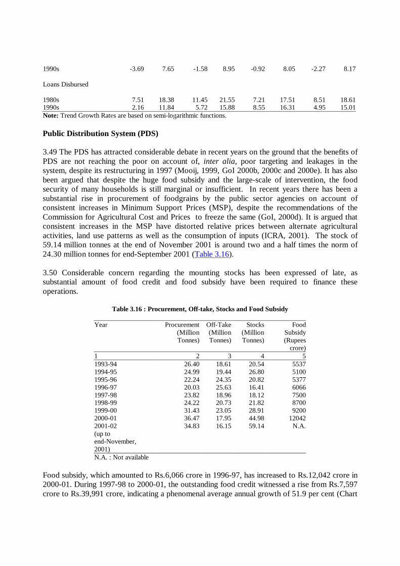
1990s -3.69 7.65 -1.58 8.95 -0.92 8.05 -2.27 8.17

Loans Disbursed

1980s 7.51 18.38 11.45 21.55 7.21 17.51 8.51 18.611990s 2.16 11.84 5.72 15.88 8.55 16.31 4.95 15.01Note: Trend Growth Rates are based on semi-logarithmic functions.

Public Distribution System (PDS)

3.49 The PDS has attracted considerable debate in recent years on the ground that the benefits ofPDS are not reaching the poor on account of, inter alia, poor targeting and leakages in thesystem, despite its restructuring in 1997 (Mooij, 1999, GoI 2000b, 2000c and 2000e). It has alsobeen argued that despite the huge food subsidy and the large-scale of intervention, the foodsecurity of many households is still marginal or insufficient. In recent years there has been asubstantial rise in procurement of foodgrains by the public sector agencies on account ofconsistent increases in Minimum Support Prices (MSP), despite the recommendations of theCommission for Agricultural Cost and Prices to freeze the same (GoI, 2000d). It is argued thatconsistent increases in the MSP have distorted relative prices between alternate agriculturalactivities, land use patterns as well as the consumption of inputs (ICRA, 2001). The stock of59.14 million tonnes at the end of November 2001 is around two and a half times the norm of24.30 million tonnes for end-September 2001 (Table 3.16).

3.50 Considerable concern regarding the mounting stocks has been expressed of late, assubstantial amount of food credit and food subsidy have been required to finance theseoperations.

Table 3.16 : Procurement, Off-take, Stocks and Food Subsidy

Year Procurement Off-Take Stocks Food(Million (Million (Million SubsidyTonnes) Tonnes) Tonnes) (Rupees

crore)1 2 3 4 51993-94 26.40 18.61 20.54 55371994-95 24.99 19.44 26.80 51001995-96 22.24 24.35 20.82 53771996-97 20.03 25.63 16.41 60661997-98 23.82 18.96 18.12 75001998-99 24.22 20.73 21.82 87001999-00 31.43 23.05 28.91 92002000-01 36.47 17.95 44.98 120422001-02 34.83 16.15 59.14 N.A.(up toend-November,2001)N.A. : Not available

Food subsidy, which amounted to Rs.6,066 crore in 1996-97, has increased to Rs.12,042 crore in2000-01. During 1997-98 to 2000-01, the outstanding food credit witnessed a rise from Rs.7,597crore to Rs.39,991 crore, indicating a phenomenal average annual growth of 51.9 per cent (Chart

III.18). The share of consumer subsidy in food subsidy has been declining over these years,indicating that much of the increase in food subsidy goes towards carrying costs. Carrying costof foodgrains increased to Rs.220.35 per quintal in 2000-01 from Rs.158.26 per quintal in 1996-97. Consumer subsidy on rice for below poverty line

(BPL) consumers declined to Rs.565.00 per quintal in July 2000 from Rs.589.33 per quintal in1997-98. Similarly, the consumer subsidy on wheat for BPL consumers decreased to Rs.415.00per quintal in July 2000 from Rs.536.35 per quintal in 1997-98. Given the present scenario, theeffectiveness of food subsidy in supporting the public distribution programme has beenquestioned (GoI, 2000e).

3.51 A gradual reduction of the food stock to scale down outstanding food credit and foodsubsidy needs to be considered. Measures to increase the off-take of foodgrains such as Food forWork Programme and increased open market sales including exports, may help to achieve theobjective of gradual scaling down of stocks. There is also a need to streamline the procedure forevaluating the quality of stocks, as this will have an impact on the outstanding advances ofcommercial banks to the Food Corporation of India.

3.52 Free and fair international trade in agricultural commodities can act as an engine of growthfor the economy as a whole. It is interesting to note that agriculture was placed for the first timeon the negotiating agenda of the Uruguay Round (1986-1993) (Box III.1).

Determinants of Agricultural Growth

3.53 In view of the many shades in the growing consensus seeking the reform of agriculture, it isuseful to undertake an empirical verification of the determinants of agricultural output in thecontext of the country specific conditions. The determinants considered for this excercise arearea under cultivation (chosen over gross sown area so as to take cognisance of the relativeimportance of various crops through explicit weights in the index), labour and "technologyindicators" such as irrigation intensity (ratio of gross irrigated to net irrigated area), cropping

intensity and ratio of area under HYV seeds to gross sown area, rainfall, and time trend.

Box III.1WTO and Indian Agriculture

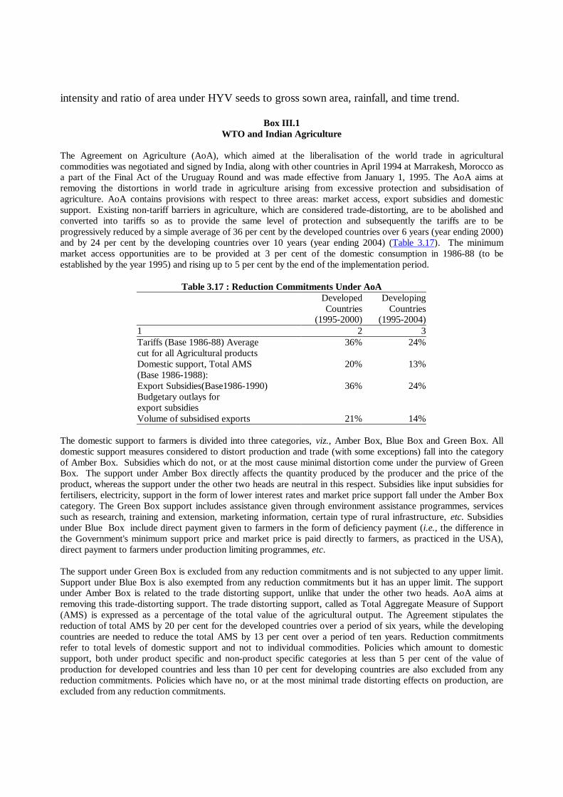
The Agreement on Agriculture (AoA), which aimed at the liberalisation of the world trade in agriculturalcommodities was negotiated and signed by India, along with other countries in April 1994 at Marrakesh, Morocco asa part of the Final Act of the Uruguay Round and was made effective from January 1, 1995. The AoA aims atremoving the distortions in world trade in agriculture arising from excessive protection and subsidisation ofagriculture. AoA contains provisions with respect to three areas: market access, export subsidies and domesticsupport. Existing non-tariff barriers in agriculture, which are considered trade-distorting, are to be abolished andconverted into tariffs so as to provide the same level of protection and subsequently the tariffs are to beprogressively reduced by a simple average of 36 per cent by the developed countries over 6 years (year ending 2000)and by 24 per cent by the developing countries over 10 years (year ending 2004) (Table 3.17). The minimummarket access opportunities are to be provided at 3 per cent of the domestic consumption in 1986-88 (to beestablished by the year 1995) and rising up to 5 per cent by the end of the implementation period.

Table 3.17 : Reduction Commitments Under AoADeveloped DevelopingCountries Countries

(1995-2000) (1995-2004)1 2 3Tariffs (Base 1986-88) Average 36% 24%cut for all Agricultural productsDomestic support, Total AMS 20% 13%(Base 1986-1988):Export Subsidies(Base1986-1990) 36% 24%Budgetary outlays forexport subsidiesVolume of subsidised exports 21% 14%

The domestic support to farmers is divided into three categories, viz., Amber Box, Blue Box and Green Box. Alldomestic support measures considered to distort production and trade (with some exceptions) fall into the categoryof Amber Box. Subsidies which do not, or at the most cause minimal distortion come under the purview of GreenBox. The support under Amber Box directly affects the quantity produced by the producer and the price of theproduct, whereas the support under the other two heads are neutral in this respect. Subsidies like input subsidies forfertilisers, electricity, support in the form of lower interest rates and market price support fall under the Amber Boxcategory. The Green Box support includes assistance given through environment assistance programmes, servicessuch as research, training and extension, marketing information, certain type of rural infrastructure, etc. Subsidiesunder Blue Box include direct payment given to farmers in the form of deficiency payment (i.e., the difference inthe Government's minimum support price and market price is paid directly to farmers, as practiced in the USA),direct payment to farmers under production limiting programmes, etc.

The support under Green Box is excluded from any reduction commitments and is not subjected to any upper limit.Support under Blue Box is also exempted from any reduction commitments but it has an upper limit. The supportunder Amber Box is related to the trade distorting support, unlike that under the other two heads. AoA aims atremoving this trade-distorting support. The trade distorting support, called as Total Aggregate Measure of Support(AMS) is expressed as a percentage of the total value of the agricultural output. The Agreement stipulates thereduction of total AMS by 20 per cent for the developed countries over a period of six years, while the developingcountries are needed to reduce the total AMS by 13 per cent over a period of ten years. Reduction commitmentsrefer to total levels of domestic support and not to individual commodities. Policies which amount to domesticsupport, both under product specific and non-product specific categories at less than 5 per cent of the value ofproduction for developed countries and less than 10 per cent for developing countries are also excluded from anyreduction commitments. Policies which have no, or at the most minimal trade distorting effects on production, areexcluded from any reduction commitments.

The developed countries are required to reduce the volume of subsidised exports by 21 per cent over six years andthe budgetary outlays for export subsidies by 36 per cent with respect to the base period of 1986-90. Developingcountries are required to reduce the volume by 14 per cent and budgetary outlays by 24 per cent over 10 years.

Implications of AoA for India

In India, quantitative restrictions on agricultural imports imposed for balance of payments (BoP) considerations havebeen removed and these imports are placed in the open general license (OGL) list. In order to provide adequateprotection to domestic producers in case of a surge in imports, India can raise the tariffs within the bound ceilings.In case of a few products such as primary products, processed products and edible oils, India had earlier raised thetariffs (during 1999 and 2000) adequately to protect the domestic producers. In case of some other products, Indiahas successfully revised the binding levels through negotiations. However, India can take suitable measures underWTO's Agreement on Safeguards if there is a serious injury to domestic producers due to surge in imports or if thereis any such other threat. The Government has already taken a number of measures to safeguard the agriculture sectorin the context of the phase-out of quantitative restriction, i.e., import duties on many agro and other items have beensubstantially increased and import of about 131 products have been subjected to compliance of mandatory Indianquality standards as applicable to domestic goods.

India's domestic support to agriculture is well below the limit of 10 per cent of the value of agricultural produce andtherefore India is not required to make any reduction in it at present. The subsidies given for PDS are basically theconsumer subsidies and are exempt from WTO discipline. India’s system of Minimum Support Prices (MSP) as alsothe provision of input subsidies to agriculture are not constrained by the Agreement. Moreover, the agriculturaldevelopmental schemes can also be continued under AoA.

Reference

1. Government of India, (2001), Focus, Ministry of Commerce.2. ________ (2001), Press Releases, Ministry of Commerce.3. ________ (2001), WTO and India, various issues, Ministry of Commerce.4. WTO (1995), Agreement on Agriculture.

3.54 Elasticities of agricultural output with respect to its various determinants are set out in Table3.18. Elasticities have been highest, predictably, with respect to area and labour, followed byrain. The elasticity of agricultural production with respect to rain at 0.27 is found to besignificant. However, the elasticities with respect to technology variables such as consumption offertiliser and pesticides, cropping intensity, irrigation intensity and the share of area under HYVseeds to gross cropped area turn out to be very low, often statistically insignificant and hence arenot reported. Inclusion of time trend taken as representative of technical progress in theestimation framework reduces the labour co-efficent apart from making it insignificant.

Table 3.18 : Estimated Elasticities of Agricultural Output

Variable Elasticity1 2 3Without Time Trend

Area 0.8243Labour 0.8618Rain 0.2667

With Time TrendArea 0.9096Labour 0.1844*Rain 0.2376

Time Trend 0.0174

* : Not significant.

3.55 Indian agriculture calls for reforms encompassing technology upgradation, creation ofinfrastructure, creation of a better marketing system, revival of the rural credit delivery system,and public sector capital formation in infrastructural facilities, particularly irrigation. In thecontext of extending reforms to agriculture, multilateral organisation have offered severalsuggestions drawn from cross-country experience (Box III.2).

Box III.2International Institutions on Reforming Agriculture

Deceleration in agricultural growth has been a common feature of the growth pattern in the Asia Pacific region inthe recent years. Global agricultural growth is also projected to decelerate to 1 per cent in 2000 after exhibitingmodest recovery in 1999 (at 2.3 per cent) over 1998 (1.4 per cent). The generally sluggish growth conditions reflecta number of underlying weaknesses which, along with uncertain weather conditions, have stifled the prospects ofagricultural growth. The underlying weaknesses continue to persist even after the observed shift in national policiesaway from public production and state administration in favour of the market.

According to the World Bank, a key aspect in the increasing market orientation of agricultural policies relates to thesequencing of agricultural reforms. Ideally, reforms that increase farmers cost of production by eliminating inputsubsidies should not precede those that can stimulate growth by raising output prices - such as elimination ofregressive price controls and export taxes. Furthermore, supply response in agriculture to reforms may not besymmetrical. An assessment based on 50 agricultural adjustment loans of the World Bank reveals that in countrieswhere agriculture was penalised/taxed, reforms helped in raising farm output. In turn, other countries whereagriculture was heavily protected, liberalisation adversely affected agricultural output growth by hasteningreallocation of resources away from agriculture. Supply response in agriculture to the overall structural reformmeasures, however, depends upon the level of agricultural development of a country. An enabling governmentpolicy may not prove very effective in the absence of adequate agricultural infrastructure - including roads,irrigation, power, and telecommunications - appropriate technology, credit, farmer education and an assured supplyof inputs at right price. Prices for inputs that do not reflect any explicit/implicit subsidy, but which are determined ina competitive market condition and also remove barriers to convergence with international prices could representgood practice in agricultural pricing policy, if not the right price. In revamping the public expenditure programmesfor agriculture as part of the overall reform process, however, countries must take adequate precaution to avoidmajor decline in agricultural growth. Recognising the underlying weaknesses of the agricultural sector in severalcountries, agricultural adjustment loans generally rely on a two prong approach. The first major aspect of theapproach emphasises price reforms and market liberalisation so as to ensure that domestic prices are in line withworld market prices, marketing and processing systems are efficient, with better access to efficient technology andpublic services. The second key aspect emphasises private production in a competitive environment.

The Asian Development Bank points out that in a market-based system for agriculture, the possibility for reapingthe potential higher yield would depend on the actual return on agricultural investment and the overall condition foragricultural production (Mingsarn, Santikarn and Benjavan Rerkasem, 2000). In the past years, decline in net returnson food crops has forced farmers to explore alternative farming opportunities with higher returns - including oilcrops, fruits and vegetables. The market mechanism, thus, seems to have altered the cropping pattern in favour ofmore profitable non-food crops. Environmental degradation - the result of faulty application of technology andagricultural policy- has, however, been a subject of concern which could threaten long-run agriculturalsustainability. In Asia, water resource management has been fragmented and project based. As a result, both surfacewater and ground water are used excessively. Crop production in fragile land has also resulted in soil erosion,salinisation, water logging and desertification. Inappropriate technology has often been used to avoid/postponereforms that may be economically and socially desirable but politically impracticable. While encouraging adoptionof any technology for the agricultural sector, therefore, due care must be taken to improve field-level knowledge,better crop management, and proper communication between farmers and research and development (R&D)

officials.

The OECD stresses the importance of the response of the labour market in agriculture to the overall process ofstructural reforms, particularly to sustain the improved labour productivity in agriculture. Surplus labor inagriculture operates as a major impediment to attain the desired labour market adjustment. It also exerts pressureson the government to address their problems through various subsidies. More efficient farm structures under marketconditions can therefore emerge only when preconditions to market efficiency could be ensured.

Keeping in view the alternative prescriptions, the future course of reforms in Indian agriculture may have to focuson the following critical areas.

? Agricultural yield can be increased through creating infrastructural facilities rather than by providing inputsubsidies. Fertiliser prices need to be streamlined further to reduce the skewed N:P:K ratio in fertiliserconsumption.

? The tools of emerging bio-technology such as genetic engineering seem to offer significant possibilities forincreasing yields. Bio-technological inputs such as bio-fertiliser and bio-pesticides are perceived to be scaleneutral and can be adopted by even small farmers and provide scope for savings on use of chemical fertilisersand pesticides, apart from being eco-friendly.

? The practice of increasing the Minimum Support Price (MSP) may have to be re-examined as it has resulted inlarge procurement of foodgrains by the public sector agencies, leading to an increase in the procurementincidentals. It has also distorted the price formation process in the market.

? In view of the removal of quantitative restrictions under the WTO agreement, the agricultural prices will have tobe aligned with the international prices to be competitive. Appropriate institutional reforms such as setting up ofcommodity exchanges are necessary to protect domestic producers from greater price volatility that generallycharacterises the international market for foodgrains and other crops.

? India is the second largest producer of fruits and vegetables in the world and is perceived to have comparativeadvantage, which needs to be reaped. Given India’s diversified climatic and soil conditions, the growingdemand for such items in the affluent parts of the world and the scope for developing the food processingindustry explains the need for shifting the pattern of production in favour of fruits and vegetables.

References

1. FAO (2001), The State of Food and Agriculture, Rome.2. Mingsarn, Santikarn Kaoshard and Benjavan Rerkasem ( 2000), Growth and Sustainability of Agriculture in

Asia, Asian Development Bank, Manila.3. OECD (1999), Agricultural Policies in Emerging Transition Economies, Vol. 1.4. World Bank (1997), "Reforming Agriculture: The World Bank Goes to Market", A World Bank Operations

Evaluation Study.

III. IMPEDIMENTS TO INDUSTRIAL GROWTH

3.56 The deceleration in economic activity in the second half of the 1990s is primarily attributedto industrial slowdown. Cyclical turns in activity have impacted on industrial output,accentuating the demand-supply imbalances. Structural factors have inhibited the growth ofcapacity creation/expansion in industry, eroded competitiveness and increased the vulnerabilityof the economy to adverse cyclical or exogenous shocks. Identified structural constraints arelack of adequate infrastructure development, low agricultural buoyancy, large fiscal imbalancesand dearth of internal reforms.

3.57 Insufficient demand is regarded as the single most important factor inhibiting growth inmanufacturing as well as other segments of the industrial sector. Apart from the globalslowdown, the current deceleration in the manufacturing sector is ascribed to slowdown ininvestments, low business confidence and subdued capital market (NCAER, 2001;

Chandrasekhar, 2001; Shetty, 2001; ADB, 2001).

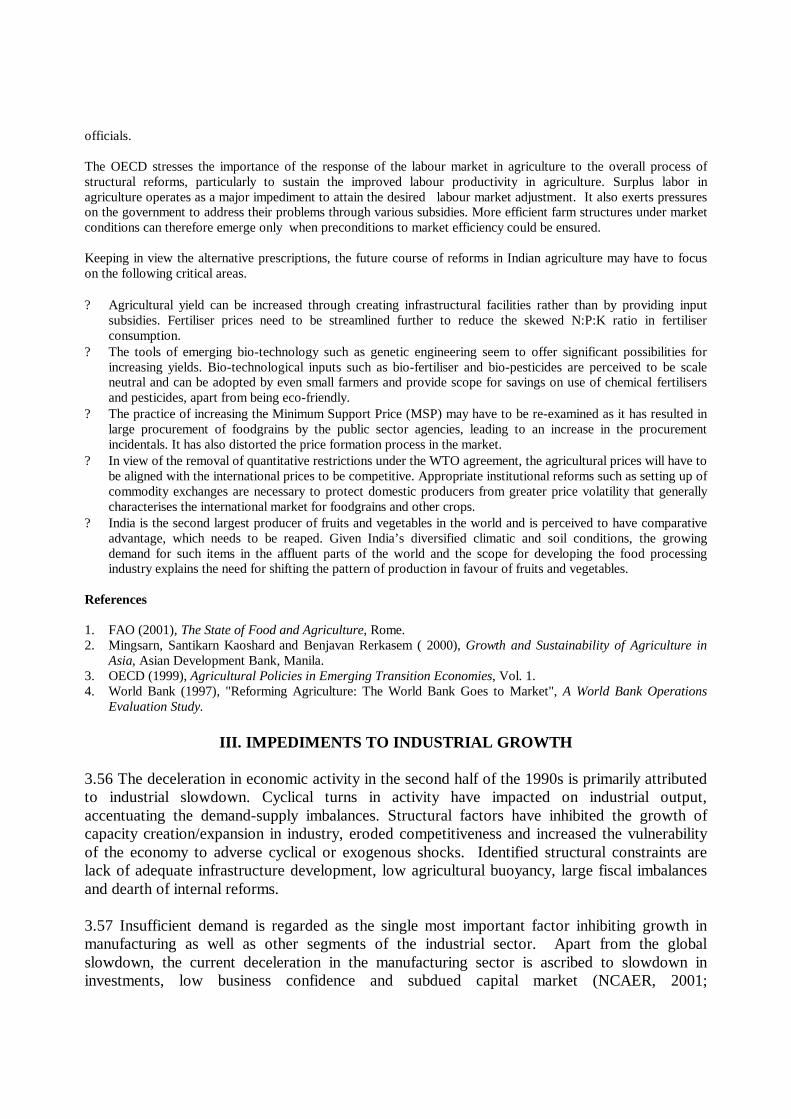
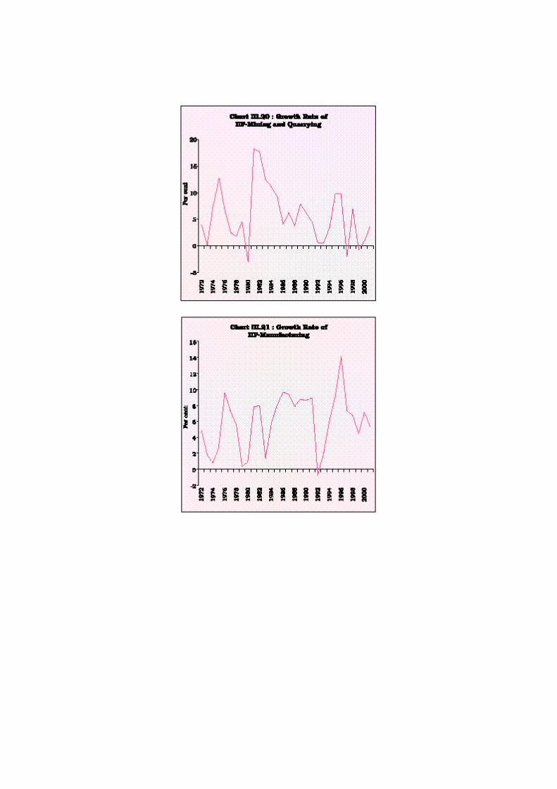
3.58 The growth of value added in the industrial sector in India slowed down in the 1990s afterrecording significant improvement in the 1980s, with similar trends at the sectoral level. Thegrowth of the industrial sector is affected by intersectoral imbalances in the growth process. Thesignificant deceleration in the growth rate of the mining and quarrying and electricity sectorsduring the 1990s affected the overall growth of industrial output. The mining and quarrying andthe manufacturing sectors have also exhibited higher volatility in the growth rate during the1990s. These fluctuations in the growth rates and imbalances across the sectors have implicationsfor stabilising output growth at higher levels (Table 3.19, 3.20 and Charts III.19, 20, 21, 22).

Table 3.19 : Trend Growth of Industrial Production in India

(Per cent)Period Mining Manufac- Electricity General

and turingQuarrying

1 2 3 4 51970-1980 4.7 4.1 7.4 4.61980-1990 7.7 7.3 8.7 7.51990-2000 3.8 6.8 6.6 6.5Note : The trend growth rates are derived from a semi- logarithimicfunction.

Table 3.20 : Coefficient of Variation of Industrial Production

(Per cent)Period Mining Manufa- Electricity General

And cturingQuarrying

1 2 3 4 51970-1980 110.1 85.0 67.4 72.91980-1990 53.0 32.3 21.2 23.71990-2000 125.1 62.2 21.4 55.7

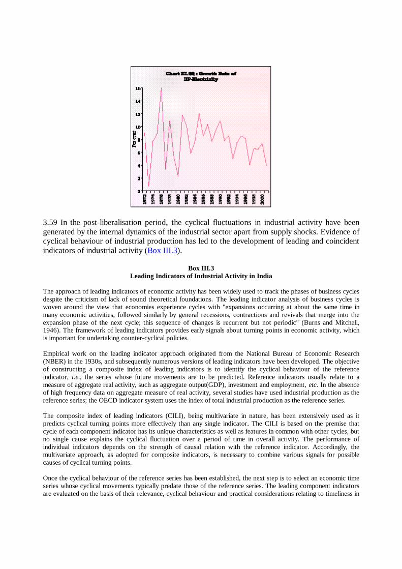
3.59 In the post-liberalisation period, the cyclical fluctuations in industrial activity have beengenerated by the internal dynamics of the industrial sector apart from supply shocks. Evidence ofcyclical behaviour of industrial production has led to the development of leading and coincidentindicators of industrial activity (Box III.3).

Box III.3Leading Indicators of Industrial Activity in India

The approach of leading indicators of economic activity has been widely used to track the phases of business cyclesdespite the criticism of lack of sound theoretical foundations. The leading indicator analysis of business cycles iswoven around the view that economies experience cycles with "expansions occurring at about the same time inmany economic activities, followed similarly by general recessions, contractions and revivals that merge into theexpansion phase of the next cycle; this sequence of changes is recurrent but not periodic" (Burns and Mitchell,1946). The framework of leading indicators provides early signals about turning points in economic activity, whichis important for undertaking counter-cyclical policies.

Empirical work on the leading indicator approach originated from the National Bureau of Economic Research(NBER) in the 1930s, and subsequently numerous versions of leading indicators have been developed. The objectiveof constructing a composite index of leading indicators is to identify the cyclical behaviour of the referenceindicator, i.e., the series whose future movements are to be predicted. Reference indicators usually relate to ameasure of aggregate real activity, such as aggregate output(GDP), investment and employment, etc. In the absenceof high frequency data on aggregate measure of real activity, several studies have used industrial production as thereference series; the OECD indicator system uses the index of total industrial production as the reference series.

The composite index of leading indicators (CILI), being multivariate in nature, has been extensively used as itpredicts cyclical turning points more effectively than any single indicator. The CILI is based on the premise thatcycle of each component indicator has its unique characteristics as well as features in common with other cycles, butno single cause explains the cyclical fluctuation over a period of time in overall activity. The performance ofindividual indicators depends on the strength of causal relation with the reference indicator. Accordingly, themultivariate approach, as adopted for composite indicators, is necessary to combine various signals for possiblecauses of cyclical turning points.

Once the cyclical behaviour of the reference series has been established, the next step is to select an economic timeseries whose cyclical movements typically predate those of the reference series. The leading component indicatorsare evaluated on the basis of their relevance, cyclical behaviour and practical considerations relating to timeliness in

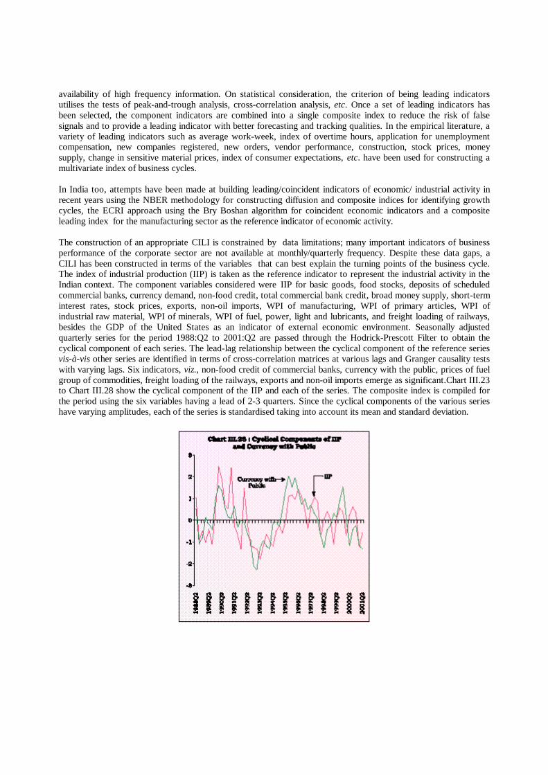
availability of high frequency information. On statistical consideration, the criterion of being leading indicatorsutilises the tests of peak-and-trough analysis, cross-correlation analysis, etc. Once a set of leading indicators hasbeen selected, the component indicators are combined into a single composite index to reduce the risk of falsesignals and to provide a leading indicator with better forecasting and tracking qualities. In the empirical literature, avariety of leading indicators such as average work-week, index of overtime hours, application for unemploymentcompensation, new companies registered, new orders, vendor performance, construction, stock prices, moneysupply, change in sensitive material prices, index of consumer expectations, etc. have been used for constructing amultivariate index of business cycles.

In India too, attempts have been made at building leading/coincident indicators of economic/ industrial activity inrecent years using the NBER methodology for constructing diffusion and composite indices for identifying growthcycles, the ECRI approach using the Bry Boshan algorithm for coincident economic indicators and a compositeleading index for the manufacturing sector as the reference indicator of economic activity.

The construction of an appropriate CILI is constrained by data limitations; many important indicators of businessperformance of the corporate sector are not available at monthly/quarterly frequency. Despite these data gaps, aCILI has been constructed in terms of the variables that can best explain the turning points of the business cycle.The index of industrial production (IIP) is taken as the reference indicator to represent the industrial activity in theIndian context. The component variables considered were IIP for basic goods, food stocks, deposits of scheduledcommercial banks, currency demand, non-food credit, total commercial bank credit, broad money supply, short-terminterest rates, stock prices, exports, non-oil imports, WPI of manufacturing, WPI of primary articles, WPI ofindustrial raw material, WPI of minerals, WPI of fuel, power, light and lubricants, and freight loading of railways,besides the GDP of the United States as an indicator of external economic environment. Seasonally adjustedquarterly series for the period 1988:Q2 to 2001:Q2 are passed through the Hodrick-Prescott Filter to obtain thecyclical component of each series. The lead-lag relationship between the cyclical component of the reference seriesvis-à-vis other series are identified in terms of cross-correlation matrices at various lags and Granger causality testswith varying lags. Six indicators, viz., non-food credit of commercial banks, currency with the public, prices of fuelgroup of commodities, freight loading of the railways, exports and non-oil imports emerge as significant.Chart III.23to Chart III.28 show the cyclical component of the IIP and each of the series. The composite index is compiled forthe period using the six variables having a lead of 2-3 quarters. Since the cyclical components of the various serieshave varying amplitudes, each of the series is standardised taking into account its mean and standard deviation.

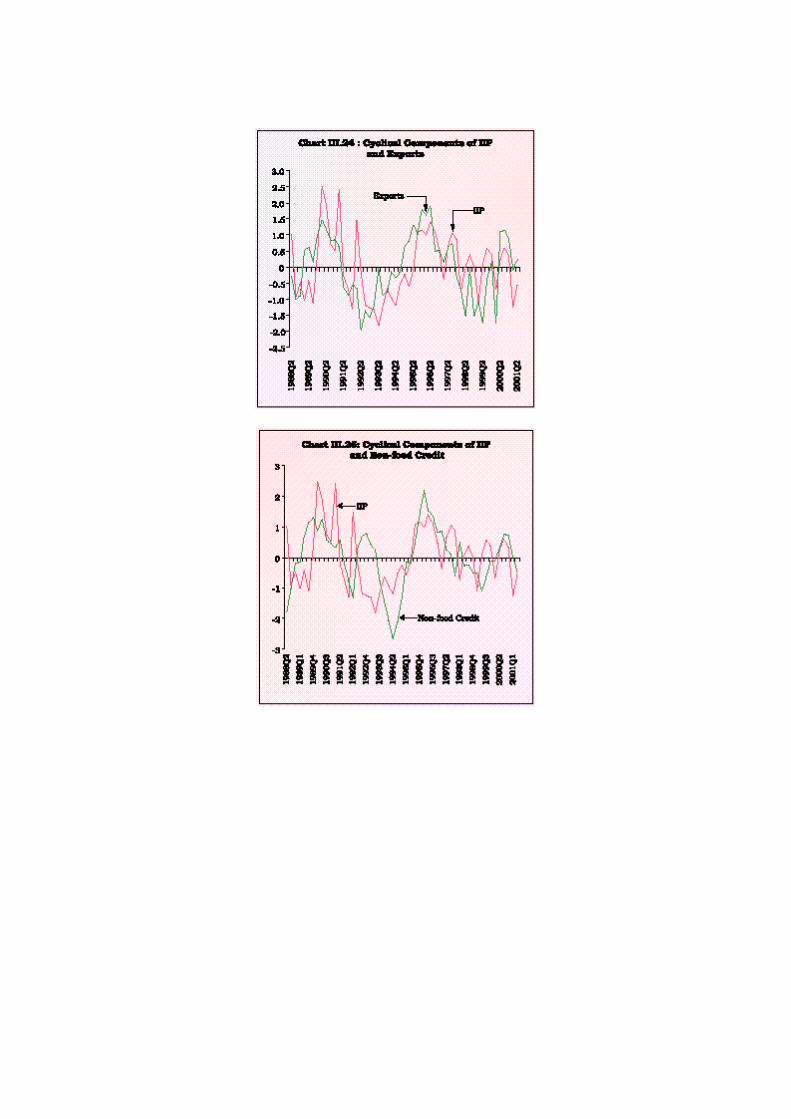
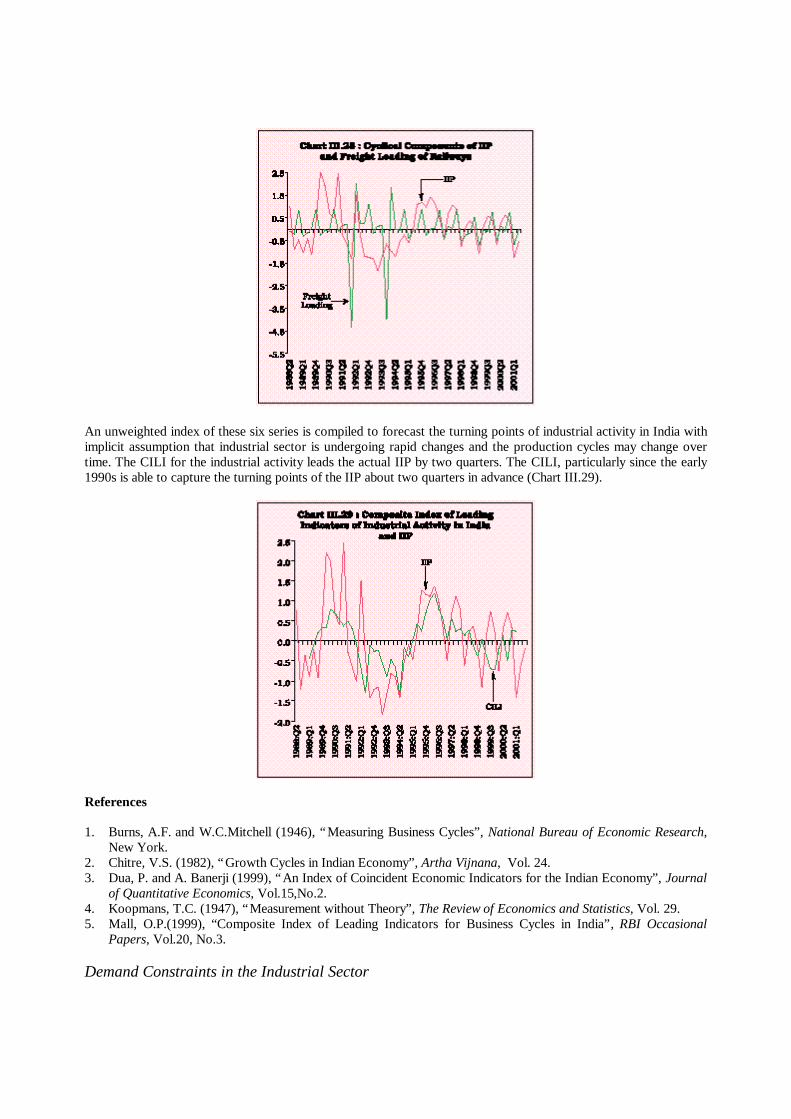
An unweighted index of these six series is compiled to forecast the turning points of industrial activity in India withimplicit assumption that industrial sector is undergoing rapid changes and the production cycles may change overtime. The CILI for the industrial activity leads the actual IIP by two quarters. The CILI, particularly since the early1990s is able to capture the turning points of the IIP about two quarters in advance (Chart III.29).

References

1. Burns, A.F. and W.C.Mitchell (1946), “Measuring Business Cycles”, National Bureau of Economic Research,New York.

2. Chitre, V.S. (1982), “Growth Cycles in Indian Economy”, Artha Vijnana, Vol. 24.3. Dua, P. and A. Banerji (1999), “An Index of Coincident Economic Indicators for the Indian Economy”, Journal

of Quantitative Economics, Vol.15,No.2.4. Koopmans, T.C. (1947), “Measurement without Theory”, The Review of Economics and Statistics, Vol. 29.5. Mall, O.P.(1999), “Composite Index of Leading Indicators for Business Cycles in India”, RBI Occasional

Papers, Vol.20, No.3.

Demand Constraints in the Industrial Sector

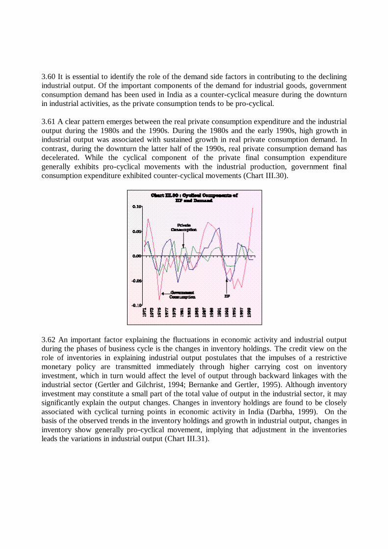
3.60 It is essential to identify the role of the demand side factors in contributing to the decliningindustrial output. Of the important components of the demand for industrial goods, governmentconsumption demand has been used in India as a counter-cyclical measure during the downturnin industrial activities, as the private consumption tends to be pro-cyclical.

3.61 A clear pattern emerges between the real private consumption expenditure and the industrialoutput during the 1980s and the 1990s. During the 1980s and the early 1990s, high growth inindustrial output was associated with sustained growth in real private consumption demand. Incontrast, during the downturn the latter half of the 1990s, real private consumption demand hasdecelerated. While the cyclical component of the private final consumption expendituregenerally exhibits pro-cyclical movements with the industrial production, government finalconsumption expenditure exhibited counter-cyclical movements (Chart III.30).

3.62 An important factor explaining the fluctuations in economic activity and industrial outputduring the phases of business cycle is the changes in inventory holdings. The credit view on therole of inventories in explaining industrial output postulates that the impulses of a restrictivemonetary policy are transmitted immediately through higher carrying cost on inventoryinvestment, which in turn would affect the level of output through backward linkages with theindustrial sector (Gertler and Gilchrist, 1994; Bernanke and Gertler, 1995). Although inventoryinvestment may constitute a small part of the total value of output in the industrial sector, it maysignificantly explain the output changes. Changes in inventory holdings are found to be closelyassociated with cyclical turning points in economic activity in India (Darbha, 1999). On thebasis of the observed trends in the inventory holdings and growth in industrial output, changes ininventory show generally pro-cyclical movement, implying that adjustment in the inventoriesleads the variations in industrial output (Chart III.31).

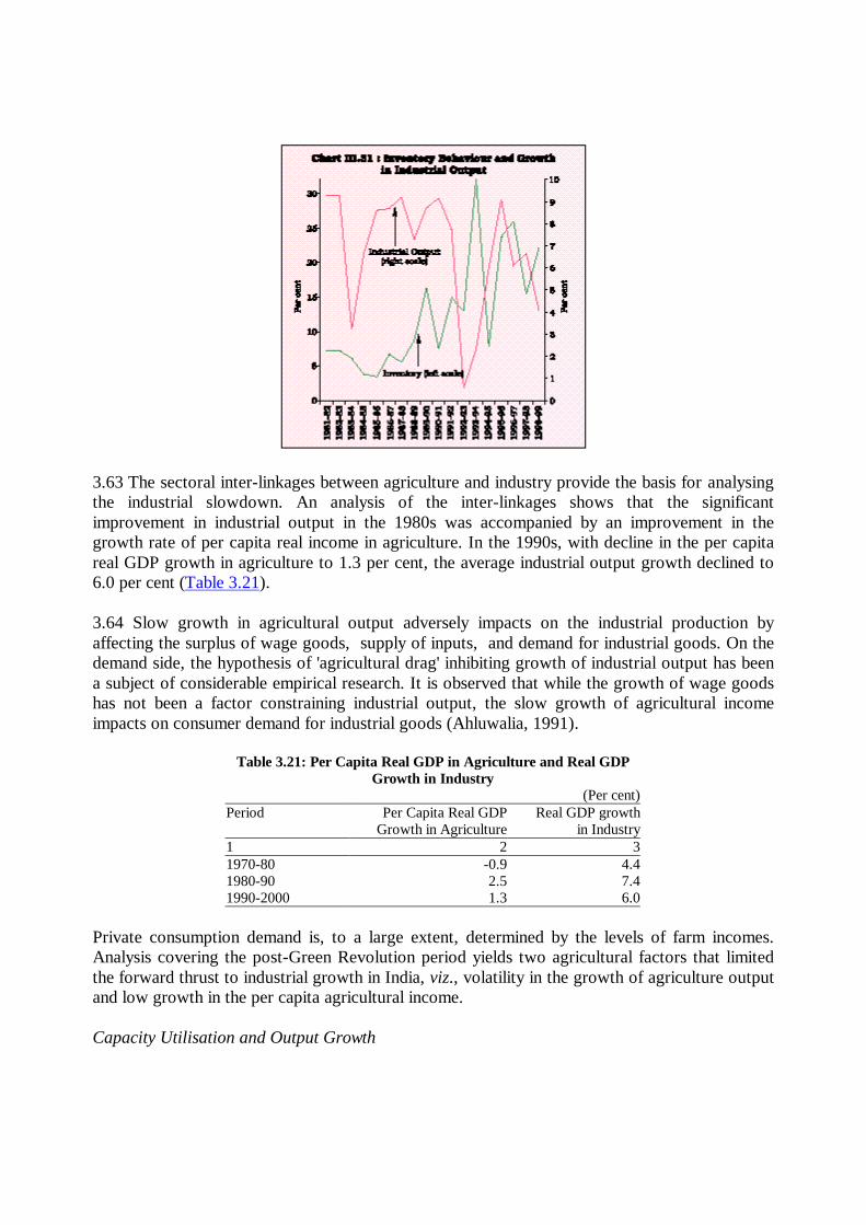
3.63 The sectoral inter-linkages between agriculture and industry provide the basis for analysingthe industrial slowdown. An analysis of the inter-linkages shows that the significantimprovement in industrial output in the 1980s was accompanied by an improvement in thegrowth rate of per capita real income in agriculture. In the 1990s, with decline in the per capitareal GDP growth in agriculture to 1.3 per cent, the average industrial output growth declined to6.0 per cent (Table 3.21).

3.64 Slow growth in agricultural output adversely impacts on the industrial production byaffecting the surplus of wage goods, supply of inputs, and demand for industrial goods. On thedemand side, the hypothesis of 'agricultural drag' inhibiting growth of industrial output has beena subject of considerable empirical research. It is observed that while the growth of wage goodshas not been a factor constraining industrial output, the slow growth of agricultural incomeimpacts on consumer demand for industrial goods (Ahluwalia, 1991).

Table 3.21: Per Capita Real GDP in Agriculture and Real GDPGrowth in Industry

(Per cent)Period Per Capita Real GDP Real GDP growth

Growth in Agriculture in Industry1 2 31970-80 -0.9 4.41980-90 2.5 7.41990-2000 1.3 6.0

Private consumption demand is, to a large extent, determined by the levels of farm incomes.Analysis covering the post-Green Revolution period yields two agricultural factors that limitedthe forward thrust to industrial growth in India, viz., volatility in the growth of agriculture outputand low growth in the per capita agricultural income.

Capacity Utilisation and Output Growth

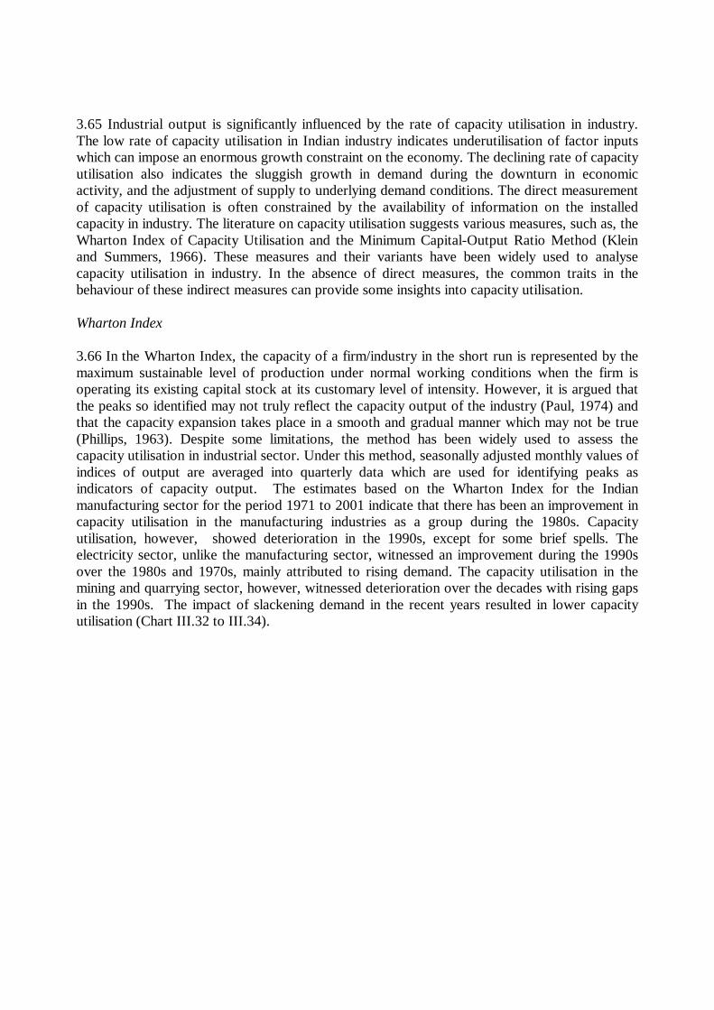
3.65 Industrial output is significantly influenced by the rate of capacity utilisation in industry.The low rate of capacity utilisation in Indian industry indicates underutilisation of factor inputswhich can impose an enormous growth constraint on the economy. The declining rate of capacityutilisation also indicates the sluggish growth in demand during the downturn in economicactivity, and the adjustment of supply to underlying demand conditions. The direct measurementof capacity utilisation is often constrained by the availability of information on the installedcapacity in industry. The literature on capacity utilisation suggests various measures, such as, theWharton Index of Capacity Utilisation and the Minimum Capital-Output Ratio Method (Kleinand Summers, 1966). These measures and their variants have been widely used to analysecapacity utilisation in industry. In the absence of direct measures, the common traits in thebehaviour of these indirect measures can provide some insights into capacity utilisation.

Wharton Index

3.66 In the Wharton Index, the capacity of a firm/industry in the short run is represented by themaximum sustainable level of production under normal working conditions when the firm isoperating its existing capital stock at its customary level of intensity. However, it is argued thatthe peaks so identified may not truly reflect the capacity output of the industry (Paul, 1974) andthat the capacity expansion takes place in a smooth and gradual manner which may not be true(Phillips, 1963). Despite some limitations, the method has been widely used to assess thecapacity utilisation in industrial sector. Under this method, seasonally adjusted monthly values ofindices of output are averaged into quarterly data which are used for identifying peaks asindicators of capacity output. The estimates based on the Wharton Index for the Indianmanufacturing sector for the period 1971 to 2001 indicate that there has been an improvement incapacity utilisation in the manufacturing industries as a group during the 1980s. Capacityutilisation, however, showed deterioration in the 1990s, except for some brief spells. Theelectricity sector, unlike the manufacturing sector, witnessed an improvement during the 1990sover the 1980s and 1970s, mainly attributed to rising demand. The capacity utilisation in themining and quarrying sector, however, witnessed deterioration over the decades with rising gapsin the 1990s. The impact of slackening demand in the recent years resulted in lower capacityutilisation (Chart III.32 to III.34).

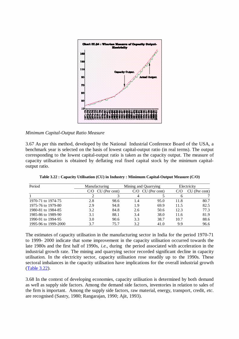
Minimum Capital-Output Ratio Measure

3.67 As per this method, developed by the National Industrial Conference Board of the USA, abenchmark year is selected on the basis of lowest capital-output ratio (in real terms). The outputcorresponding to the lowest capital-output ratio is taken as the capacity output. The measure ofcapacity utilisation is obtained by deflating real fixed capital stock by the minimum capital-output ratio.

Table 3.22 : Capacity Utilisation (CU) in Industry : Minimum Capital-Output Measure (C/O)

Period Manufacturing Mining and Quarrying ElectricityC/O CU (Per cent) C/O CU (Per cent) C/O CU (Per cent)

1 2 3 4 5 6 71970-71 to 1974-75 2.8 98.6 1.4 95.0 11.8 80.71975-76 to 1979-80 2.9 94.8 1.9 69.9 11.5 82.51980-81 to 1984-85 3.2 84.8 2.6 50.6 12.3 77.31985-86 to 1989-90 3.1 88.1 3.4 38.0 11.6 81.91990-91 to 1994-95 3.0 90.6 3.3 38.7 10.7 88.61995-96 to 1999-2000 3.7 75.7 3.2 41.0 9.9 96.6

The estimates of capacity utilisation in the manufacturing sector in India for the period 1970-71to 1999- 2000 indicate that some improvement in the capacity utilisation occurred towards thelate 1980s and the first half of 1990s, i.e., during the period associated with acceleration in theindustrial growth rate. The mining and quarrying sector recorded significant decline in capacityutilisation. In the electricity sector, capacity utilisation rose steadily up to the 1990s. Thesesectoral imbalances in the capacity utilisation have implications for the overall industrial growth(Table 3.22).

3.68 In the context of developing economies, capacity utilisation is determined by both demandas well as supply side factors. Among the demand side factors, inventories in relation to sales ofthe firm is important. Among the supply side factors, raw material, energy, transport, credit, etc.are recognised (Sastry, 1980; Rangarajan, 1990; Ajit, 1993).

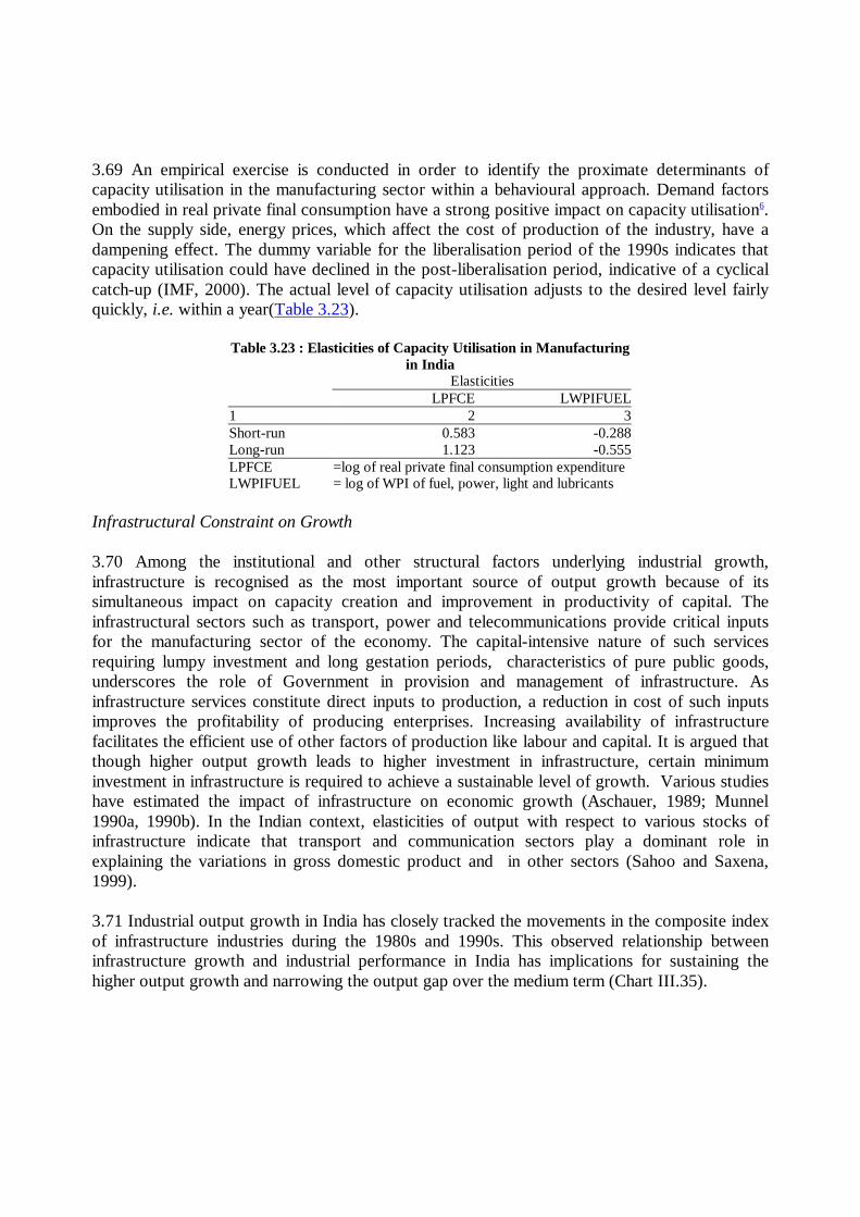
3.69 An empirical exercise is conducted in order to identify the proximate determinants ofcapacity utilisation in the manufacturing sector within a behavioural approach. Demand factorsembodied in real private final consumption have a strong positive impact on capacity utilisation6.On the supply side, energy prices, which affect the cost of production of the industry, have adampening effect. The dummy variable for the liberalisation period of the 1990s indicates thatcapacity utilisation could have declined in the post-liberalisation period, indicative of a cyclicalcatch-up (IMF, 2000). The actual level of capacity utilisation adjusts to the desired level fairlyquickly, i.e. within a year(Table 3.23).

Table 3.23 : Elasticities of Capacity Utilisation in Manufacturingin India

ElasticitiesLPFCE LWPIFUEL

1 2 3Short-run 0.583 -0.288Long-run 1.123 -0.555LPFCE =log of real private final consumption expenditureLWPIFUEL = log of WPI of fuel, power, light and lubricants

Infrastructural Constraint on Growth

3.70 Among the institutional and other structural factors underlying industrial growth,infrastructure is recognised as the most important source of output growth because of itssimultaneous impact on capacity creation and improvement in productivity of capital. Theinfrastructural sectors such as transport, power and telecommunications provide critical inputsfor the manufacturing sector of the economy. The capital-intensive nature of such servicesrequiring lumpy investment and long gestation periods, characteristics of pure public goods,underscores the role of Government in provision and management of infrastructure. Asinfrastructure services constitute direct inputs to production, a reduction in cost of such inputsimproves the profitability of producing enterprises. Increasing availability of infrastructurefacilitates the efficient use of other factors of production like labour and capital. It is argued thatthough higher output growth leads to higher investment in infrastructure, certain minimuminvestment in infrastructure is required to achieve a sustainable level of growth. Various studieshave estimated the impact of infrastructure on economic growth (Aschauer, 1989; Munnel1990a, 1990b). In the Indian context, elasticities of output with respect to various stocks ofinfrastructure indicate that transport and communication sectors play a dominant role inexplaining the variations in gross domestic product and in other sectors (Sahoo and Saxena,1999).

3.71 Industrial output growth in India has closely tracked the movements in the composite indexof infrastructure industries during the 1980s and 1990s. This observed relationship betweeninfrastructure growth and industrial performance in India has implications for sustaining thehigher output growth and narrowing the output gap over the medium term (Chart III.35).

3.72 Empirical evidence points to a robust relationship between infrastructure investment andproductivity growth in the manufacturing sector (Ahluwalia, 1991). The high growthperformance of infrastructure sector during the 1980s can be attributed to a strong resurgence inthe growth of infrastructure investment during the Sixth and the Seventh Plans. The public sectordominates in the power sector, water supply, railways and roads, etc., while the private sector ispredominantly in the transport sector, mainly road cargo transport. The India InfrastructureReport (1996) projected infrastructure investment requirement at 8.0 per cent of GDP over amedium term (Table 3.24). The requirements of funds for infrastructure are estimated to rise andan increasing proportion of gross domestic investment would have to be earmarked for financingthe infrastructure.

Table 3.24 : Projected Investment Requirements forInfrastructure (Macro Estimates)

(Rupees billion)Year Gross GDI in GDI in GDI in

Domestic Infrast- Infrastr- Infrastr-Investment ructure ucture ucture

(GDI) as % as % of -of GDP total GDI

1 2 3 4 51990-91 1448.5 287.4 5.4 19.81995-96 2825.5 598.6 5.5 21.22000-01 4512.0 1076.0 7.0 23.82003-04 5938.8 1472.3 7.6 24.82004-05 6523.4 1639.0 7.8 25.12005-06 7179.5 1826.1 8.0 25.4

Note : The data for GDP, Projected GDI and GDI in infrastructurefrom 1995-96 onwards are at1995-96 prices.

Source: The India Infrastructure Report (1996)

Sectoral Imbalances and Gaps in Infrastructure

3.73 Sectoral imbalances in infrastructure impose constraints on the growth of industrial output.

Juxtaposed with the slowdown in the growth of the infrastructure sector between the 1980s and1990s, the persistence of sectoral imbalances in the infrastructure sub-sectors has simultaneouslyposed challenges for capacity expansion as well as utilisation of the existing capacity. Thesectoral performance during the 1990s reveals that the average growth of all infrastructureindustries, except for the steel sector, has remained significantly lower than in the 1980s. Thedecline in the overall growth of infrastructure sector in the 1990s in relation to the 1980semanated mainly from a decline in growth of electricity, coal and petroleum. The stylised factshighlight the importance of the energy sector in sustaining higher growth of industrial output(Chart III.36, 37, 38, 39, 40).

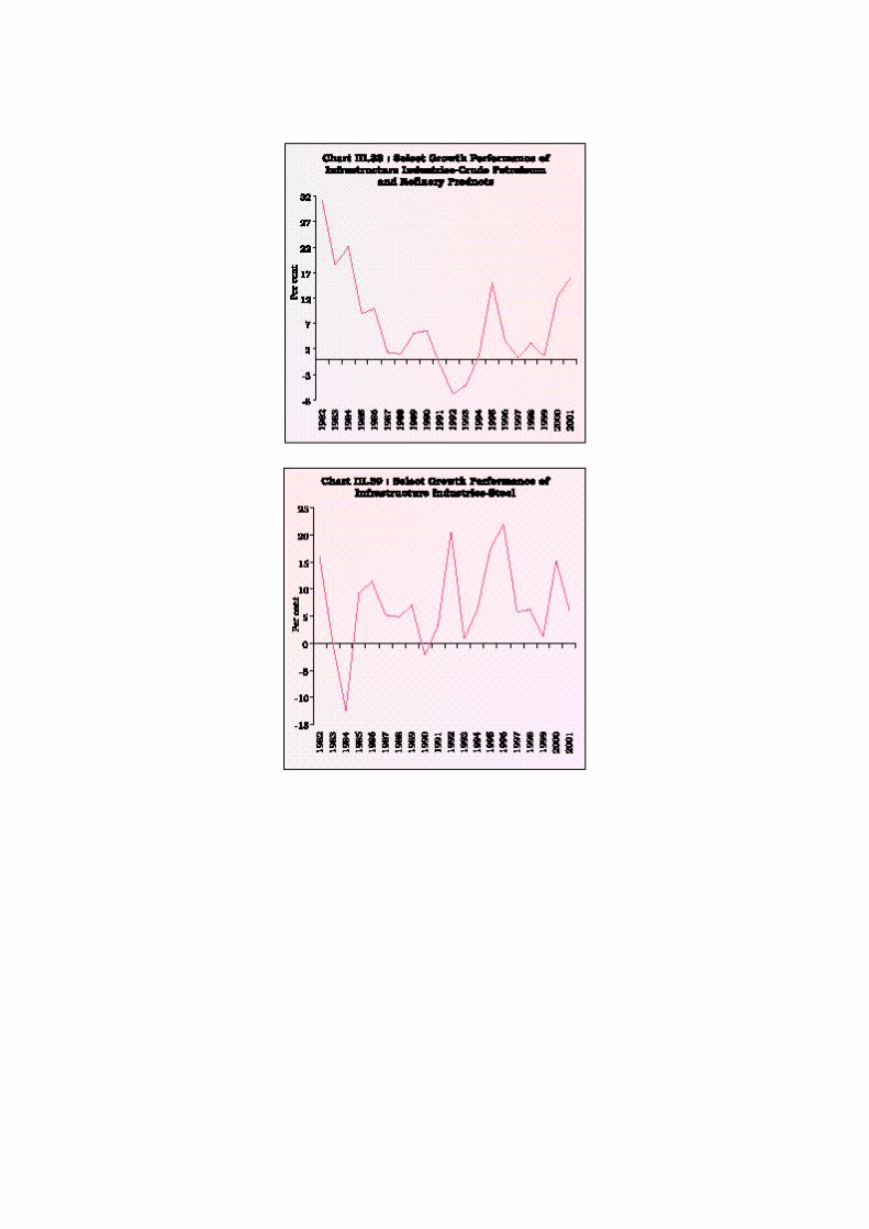
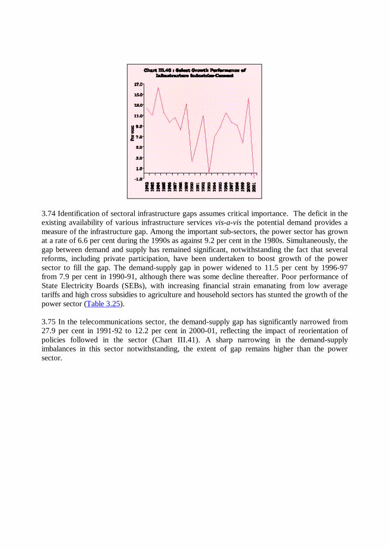
3.74 Identification of sectoral infrastructure gaps assumes critical importance. The deficit in theexisting availability of various infrastructure services vis-a-vis the potential demand provides ameasure of the infrastructure gap. Among the important sub-sectors, the power sector has grownat a rate of 6.6 per cent during the 1990s as against 9.2 per cent in the 1980s. Simultaneously, thegap between demand and supply has remained significant, notwithstanding the fact that severalreforms, including private participation, have been undertaken to boost growth of the powersector to fill the gap. The demand-supply gap in power widened to 11.5 per cent by 1996-97from 7.9 per cent in 1990-91, although there was some decline thereafter. Poor performance ofState Electricity Boards (SEBs), with increasing financial strain emanating from low averagetariffs and high cross subsidies to agriculture and household sectors has stunted the growth of thepower sector (Table 3.25).

3.75 In the telecommunications sector, the demand-supply gap has significantly narrowed from27.9 per cent in 1991-92 to 12.2 per cent in 2000-01, reflecting the impact of reorientation ofpolicies followed in the sector (Chart III.41). A sharp narrowing in the demand-supplyimbalances in this sector notwithstanding, the extent of gap remains higher than the powersector.

Table 3.25 : Demand-Supply Gap in the Power Sector in India(Million units)

Year Requirement Availability Deficit Deficitas % of

Requirement1 2 3 4 51990-91 2,67,632 2,46,560 21,072 7.91991-92 2,88,974 2,66,432 22,542 7.81992-93 3,05,266 2,79,824 25,442 8.31993-94 3,23,252 2,99,494 23,758 7.31994-95 3,52,260 3,27,281 24,979 7.11995-96 3,89,721 3,54,045 35,676 9.21996-97 4,13,490 3,65,900 47,590 11.51997-98 4,24,505 3,90,330 34,175 8.11998-99 4,46,584 4,20,235 26,349 5.91999-2000 4,80,430 4,50,594 29,836 6.22000-01 5,07,213 4,67,401 39,812 7.8Source: Annual Reports, Ministry of Power, Governmentof India, various issues.

Although entry of the private sector has led to some increase in service expansion, the rollout ofservices has not begun as quickly as expected. The existing gaps in the telecom sector haveimplications for the technical efficiency and productivity growth in the industrial sector.

3.76 The role of public capital in infrastructure in explaining the growth in productivity andoutput is well recognised. Keeping in view the stylised facts on the performance of infrastructureand demand-supply mismatches, the role of public capital in mitigating these gaps needs someassessment. With a view to exploring the role of public capital in infrastructure in explaining theoutput growth, a logarithmic form of the Cobb-Douglas production function for themanufacturing sector is estimated with public capital stock as an additional argument (ChartIII.42). The public capital in infrastructure emerges as the most dominant factor in explainingoutput growth in the manufacturing sector with a positive elasticity of 0.76. These estimateshighlight the role of public infrastructure investment in sustaining higher output growth in the

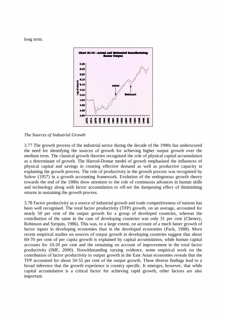
long term.

The Sources of Industrial Growth

3.77 The growth process of the industrial sector during the decade of the 1990s has underscoredthe need for identifying the sources of growth for achieving higher output growth over themedium term. The classical growth theories recognised the role of physical capital accumulationas a determinant of growth. The Harrod-Domar model of growth emphasised the influences ofphysical capital and savings in creating effective demand as well as productive capacity inexplaining the growth process. The role of productivity in the growth process was recognised bySolow (1957) in a growth accounting framework. Evolution of the endogenous growth theorytowards the end of the 1980s drew attention to the role of continuous advances in human skillsand technology along with factor accumulation to off-set the dampening effect of diminishingreturns in sustaining the growth process.

3.78 Factor productivity as a source of industrial growth and trade competitiveness of nations hasbeen well recognised. The total factor productivity (TFP) growth, on an average, accounted fornearly 50 per cent of the output growth for a group of developed countries, whereas thecontribution of the same in the case of developing countries was only 31 per cent (Chenery,Robinson and Syrquin, 1986). This was, to a large extent, on account of a much faster growth offactor inputs in developing economies than in the developed economies (Pack, 1988). Morerecent empirical studies on sources of output growth in developing countries suggest that about60-70 per cent of per capita growth is explained by capital accumulation, while human capitalaccounts for 10-20 per cent and the remaining on account of improvement in the total factorproductivity (IMF, 2000). Notwithstanding varying evidence, some empirical work on thecontribution of factor productivity to output growth in the East Asian economies reveals that theTFP accounted for about 50-55 per cent of the output growth. These diverse findings lead to abroad inference that the growth experience is country specific. It emerges, however, that whilecapital accumulation is a critical factor for achieving rapid growth, other factors are alsoimportant.

3.79 In the Indian manufacturing sector, the analysis of the sources of growth between 1959-60to 1985-86 indicates that overall long-term annual growth of 5.3 per cent in value added in themanufacturing sector was associated with rapid growth of capital (8 per cent), moderate growthof employment (3 per cent) and negative growth in TFP at 0.4 per cent (Ahluwalia, 1991). Thesefindings suggest that till the mid-1980s, the entire growth was led mainly by the capitalaccumulation and the contribution of productivity growth was negligible, reflecting the lowefficiency of factor use. A synoptic view of the studies conducted on the Indian manufacturingsector indicates that even though an increasing trend in labour productivity has been witnessed incase of most of the industry groups, the level of labour productivity in India is abysmally lowand its convergence to international standards seems to be a difficult proposition in the nearfuture (Table 3.26).

3.80 In these studies, factor productivity growth obtained through the single deflation approachis lower than the double deflation approach, implying that the relative prices of inputs and outputhave increased over time7. Firm level panel evidence, however, indicates a strong evidence of adecline in productivity growth rates in the 1990s as compared with the 1980s. Productivitygrowth of firms in the manufacturing sector could have been adversely affected by the poorperformance of the efficiency component in productivity (NCAER, 2001). For small-scaleindustries, there is a decline in labour productivity growth during the1990s (1990-96) to 3.7 percent from 6.2 per cent in the 1980s and a decline in capital productivity growth to -1.6 per centfrom 2.6 per cent during the same period (SIDBI, 2000).

Table 3.26 : Trends in Factor Productivity in the Manufacturing Sector in India- Alternative Estimates(Per cent per annum)

Study Period Covered TFPG (Single TFPG(DoubleDeflation Method) Deflation Method)

1 2 3 4Brahmananda (1982) 1950-51 to 1980-81 -0.2Ahluwalia (1985) 1959-60 to 1979-80 -0.6Ahluwalia (1991) 1959-60 to 1985-86 -0.4Balakrishnan and Pushpangadan (1994) 1970-71 to 1988-89 0.5 3.1Majumdar (1996) 1950-51 to 1992-93 1.7*Rao, M.J. (1996) 1973-74 to 1992-93 1.3@ 2.2Pradhan and Barik (1998) 1963-64 to 1992-93 0.6Trivedi et al (2000) 1973-74 to 1997-98 1.95 3.7NCAER (2001) 1980-81 to 1996-97 -0.05 to 0.04#

* The estimates are reported only for the sub-period 1973-74 to 1992-93, out of the total period of the studyspanning 1950-51 to 1992-93.

@ Growth rate of TFP is obtained indirectly from the estimates of TPG.# Represent different econometric estimates of TFPG based on the firm level panel data set.

3.81 In the context of the growing degree of openness of the economy, the level and growth ratesof productivity of labour and capital have to be compared with some benchmark levels.Comparative levels of value added per person in manufacturing in 1987 revealed that for India,the ratio was only 7.2 per cent of that of the United States and 10.3 per cent of that of the WestGermany (Ark, 1996). This indicates that the level of productivity in India is relatively low andwould require considerable improvement to achieve convergence to the international levels.

3.82 Sources of productivity growth in India could broadly comprise infrastructure, reorientationin the trade and industrial policies, foreign direct investment along with technology transfers,reforms in the labour market to impart necessary flexibility and supply response, changes in exitprocedures through appropriate legislation on industrial sickness, the Companies Act andindustrial disputes and bankruptcy laws. The supply side response would depend upon raisinginvestment in infrastructure, hastening of disinvestment process and restructuring of publicenterprises.

Technological Progress and Industrial Growth

3.83 Productivity growth is the combined effect of pure technical progress as well as theimprovement in the overall efficiency of factor use. Technological change involves animprovement in technology, knowledge and work efficiency. Technological progress isrecognised as the key to maintaining productivity growth, and the driving force behind economicgrowth (Solow, 1957).

3.84 Attempts have been made in recent years to examine the role of technology expenditure ongrowth of productivity and output. Empirical findings support the view that science andtechnology play a critical role in the growth process of major industrialised countries(Sveikauskas, 1983). The hypothesis that research and development (R&D) fosters productivitygrowth through advances in technology has also gained support at the empirical level (Scherer,1983). While explaining the differences in growth rates of labour productivity in theindustrialised countries, it is found that technological development in the form of the growth ofR&D expenditures and technology gap explain the growth rate of labour productivity in theindustrial countries (Rensman and Kuper, 2000). In the case of newly industrialised countries,rapid growth in productivity and output is found to be the outcome of the ability to acquireadvanced technology (Rothwell and Zegveld, 1985). These findings have important implicationsfor the developing countries aiming for higher productivity growth since technological progressis based mainly on the import of technology.

3.85 Given that the Indian firms do not spend much on R&D, import of capital goods andmachinery has had a significant impact on corporate performance. Capital deepening (i.e., rise incapital-output ratio) was not found to be favouring the performance of larger firms, implying thatup to a certain point, capital deepening might help growth and profits, beyond that furtherincreases in the capital-sales ratio prove counterproductive to growth and profits (Siddharthan,1992). These empirical findings, though relate to the pre-liberalisation period, lend support to therole of technological progress in enhancing productivity and growth. In the context of thetechnology gap in Indian industry during the 1980s, the per firm expenditure on technologyimports revealed a steady rise, while the R&D expenditure continued to remain meagre(Swaminathan, 1993).

3.86 The impact of the reform process on technological improvement can be evaluated bycomparing these indicators to the outcome of the 1990s. In the case of public limited companiesin India, the ratio of R&D expenditure to their total output was as low as 0.08 per cent in 1985-86, increasing to 0.31 per cent in 1990-91 and remaining almost at that level in 1999-2000. Thisreflects considerably low level of R&D expenditure in the production process as compared with

industrialised countries. One of the factors for inadequate growth in R&D expenditure during thepost-liberalisation period is the liberalisation of technology import and foreign investment policy(Table 3.27).

3.87 The sectoral break up of R&D expenditure suggests that the maximum investments arerecorded in chemical and pharmaceutical groups, followed by engineering, motor vechicles,transport and information technology. The R&D expenditure on electricity generation and supplywitnessed sharp decline during the 1990s. The low level of R&D expenditure in the Indianindustry may have implications for productivity growth, competitiveness and exportperformance; however, the unfavourable impact can be, to a certain extent, mitigated throughtechnology imports and foreign collaboration.

Table 3.27 : Research and Development Expenditure in Public Limited Companies(Per cent of total output)

Industry 1985-86 1990-91 1995-96 1999-20001 2 3 4 5Aggregate 0.08 0.31 0.28 0.29

1. Tea,Sugar, Jute 0.02 0.09 0.1 0.042. Cotton Textile & Rayon 0.01 0.05 0.13 0.083. Engineering, Motor vehicles, Transport etc. 0.11 0.38 0.31 0.314. Chemicals & Pharmaceuticals etc. 0.08 0.33 0.39 0.395. Cement 0.04 0.16 0.11 0.126. Rubber and Paper Products 0.05 0.2 0.2 0.237. Electricity Generation and Supply — 0.53 0.07 0.018. Information & Technology — — — 0.28Source: Selected Financial Statistics of Public Limited Companies, RBI

3.88 An important feature of technological progress in India since 1991 has been the growth inforeign collaborations. The Indian experience shows that FDI has increasingly moved intopriority areas such as power generation, oil refining, telecommunications, electronics and foodprocessing, i.e., the sectors where domestic investment is inadequate. The trends in FDI inflowreflect an increasing trend in the 1990s; however, FDI inflows to India continue to remainmarginal when compared with the aggregate flow to the emerging economies and the gapbetween FDI approvals and actual inflows continues to remain wide (Table 3.28).

Table 3.28 : Number of Foreign Collaboration Approvals and FDI

Year No. of FDI in India FDI to All FDI to India asForeign (US $ Million) Developing % of FDI to all

Collaboration Countries Developingapprovals (US $ Million) Countries

1 2 3 4 51981 389 92 12293 0.71986 957 118 9482 1.21991 950 74 35494 0.21992 1520 277 47130 0.61993 1476 550 66574 0.81994 1854 973 90036 1.11995 2337 2144 106990 2.01996 - 2426 131451 1.81997 - 3577 172571 2.1

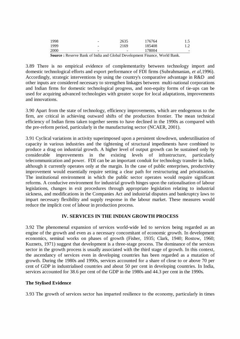
1998 - 2635 176764 1.51999 - 2169 185408 1.22000 - - 178004 -Source : Reserve Bank of India and Global Development Finance, World Bank.

3.89 There is no empirical evidence of complementarity between technology import anddomestic technological efforts and export performance of FDI firms (Subrahmanian, et al,1996).Accordingly, strategic interventions by using the country's comparative advantage in R&D andother inputs are considered necessary to strengthen linkages between multi-national corporationsand Indian firms for domestic technological progress, and non-equity forms of tie-ups can beused for acquiring advanced technologies with greater scope for local adaptations, improvementsand innovations.

3.90 Apart from the state of technology, efficiency improvements, which are endogenous to thefirm, are critical in achieving outward shifts of the production frontier. The mean technicalefficiency of Indian firms taken together seems to have declined in the 1990s as compared withthe pre-reform period, particularly in the manufacturing sector (NCAER, 2001).

3.91 Cyclical variations in activity superimposed upon a persistent slowdown, underutilisation ofcapacity in various industries and the tightening of structural impediments have combined toproduce a drag on industrial growth. A higher level of output growth can be sustained only byconsiderable improvements in the existing levels of infrastructure, particularlytelecommunication and power. FDI can be an important conduit for technology transfer in India,although it currently operates only at the margin. In the case of public enterprises, productivityimprovement would essentially require setting a clear path for restructuring and privatisation.The institutional environment in which the public sector operates would require significantreforms. A conducive environment for industrial growth hinges upon the rationalisation of labourlegislations, changes in exit procedures through appropriate legislation relating to industrialsickness, and modifications in the Companies Act and industrial disputes and bankruptcy laws toimpart necessary flexibility and supply response in the labour market. These measures wouldreduce the implicit cost of labour in production process.

IV. SERVICES IN THE INDIAN GROWTH PROCESS

3.92 The phenomenal expansion of services world-wide led to services being regarded as anengine of the growth and even as a necessary concomitant of economic growth. In developmenteconomics, seminal works on phases of growth (Fisher, 1935; Clark, 1940; Rostow, 1960;Kuznets, 1971) suggest that development is a three-stage process. The dominance of the servicessector in the growth process is usually associated with the third stage of growth. In this context,the ascendancy of services even in developing countries has been regarded as a mutation ofgrowth. During the 1980s and 1990s, services accounted for a share of close to or above 70 percent of GDP in industrialised countries and about 50 per cent in developing countries. In India,services accounted for 38.6 per cent of the GDP in the 1980s and 44.3 per cent in the 1990s.

The Stylised Evidence

3.93 The growth of services sector has imparted resilience to the economy, particularly in times

of adverse agricultural shocks as also during cyclical downturns in industry. The share ofservices sector has been steadily increasing, with a fairly rapid growth in the 1990s (Table 3.29and Chart III.43).

Table 3.29 : Sector-wise Average Shares, Growth Rates and Contribution to GDP Growth(Per cent)

Services Industry# AgriculturePeriod Share Growth Contribution Share Growth Contribution Share Growth Contribution

in Rate to GDP in Rate to GDP in Rate to GDPGDP Growth GDP Growth GDP Growth

1 2 3 4 5 6 7 8 9 101950-51 to 1959-60* 28.2 4.1 32.2 16.0 5.7 25.3 56.0 2.3 42.51960-61 to 1969-70 31.4 4.9 38.1 21.1 6.5 32.9 47.8 2.5 29.21970-71 to 1979-80 34.4 4.5 52.7 22.8 3.7 28.7 42.8 1.3 18.61980-81 to 1989-90 38.6 6.6 43.6 25.0 6.8 28.9 36.4 4.4 27.51990-91 to 2000-01 44.3 7.6 57.6 27.1 5.9 27.6 28.6 2.9 14.8# Inclusive of construction* 9 year data for growth and weighted contribution since data for 1949-50 are not available.

Due to rounding off, sectoral data may not add up to 100.Source : National Accounts Statistics, CSO.

3.94 The weighted contribution of the services sector to GDP growth has been rising since the1960s except during the 1980s when industry and agriculture recorded substantial acceleration,which led to erosion in their contribution to GDP growth. However, a resurgence of services inthe 1990s with a growth of 7.6 per cent enabled services sector to contribute 57.6 per cent toGDP growth.

3.95 A notable feature of the structural transformation of the services sector has been the growthof skill intensive and high value added sectors, i.e., software, communication and financialservices. The rapid growth of services can be attributed, inter alia, to the advent of informationtechnology (IT) and the knowledge economy. This has enhanced the growth of the highproductivity segment of the services sector as well as a variety of service activities involving lowproductivity activities catering to a large mass of people. The phenomenal growth of low skilled

service activities has occurred due to reduced opportunities in the manufacturing sector,particularly in the unorganised sectors.

3.96 Trade, hotels, restaurants and transport and communication are the major segments in termsof their share within the services sector; however, their share in the value added in the servicessector has remained constant at around 49 per cent during the 1970s and 1980s, beforemarginally declining in 1990s. The share of finance, insurance, real estate and business serviceswitnessed significant improvement during the 1990s on account of the rapid pace of financialdevelopment (Chart III.44 and Table 3.30). The buoyancy in the services sector output isconcentrated in the new economy sectors such as computer software and financial and businessservices. In the national income accounts, the contribution of the software industry in the realGDP is estimated at 0.78 per cent in 1999-2000. If raw materials in this sector are accounted for,contribution of the software sector (net of inputs) to GDP stands at about 1 per cent as per theestimates of the NASSCOM and the CMIE.

Table 3.30 : Average Share of Sub-sectors in Services Value-added (atconstant prices)

(Per cent)Period Trade, Finance, Social and

Hotels, Insurance, PersonalTransport and Real estate and services

Communi- Businesscation services

1 2 3 41950-51 to 1959-60 44.3 23.0 32.81960-61 to 1969-70 48.2 19.5 32.31970-71 to 1979-80 49.1 18.4 32.51980-81 to 1989-90 48.7 20.4 30.91990-91 to 2000-01 46.3 26.1 27.1

3.97 Some of the activities in the services sector are multidimensional, being part of industry aswell as services, such as information technology and construction. Service statistics in most

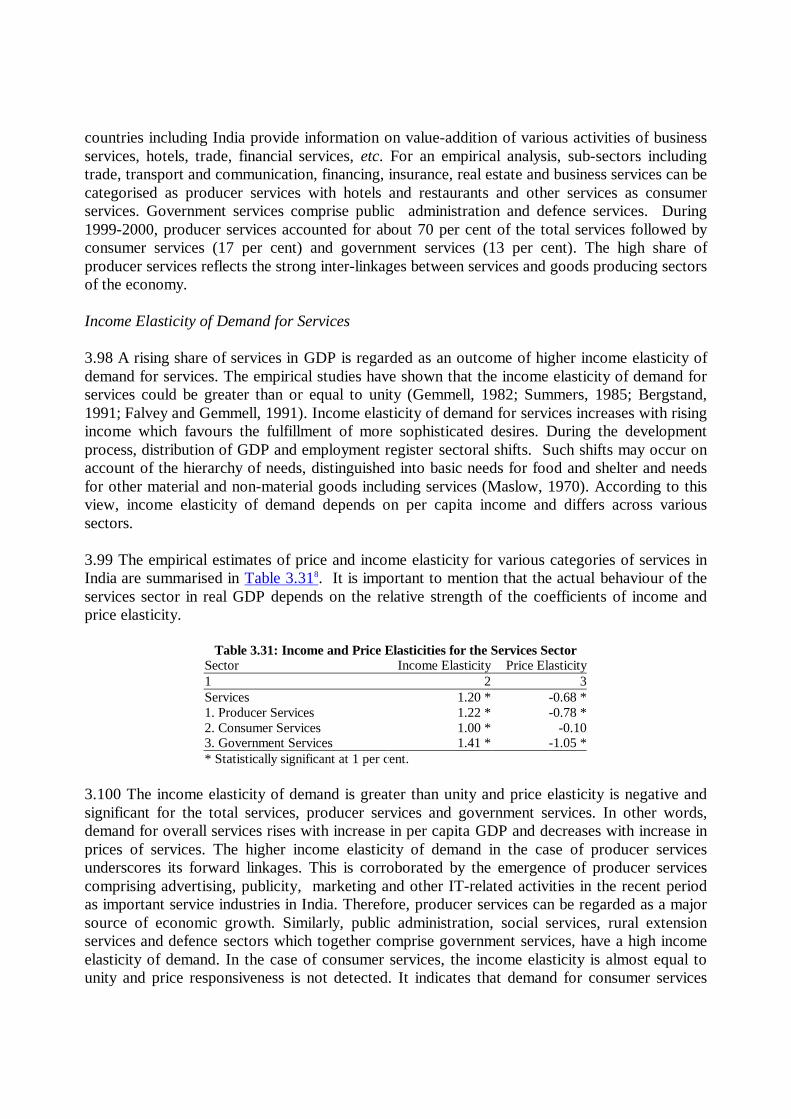
countries including India provide information on value-addition of various activities of businessservices, hotels, trade, financial services, etc. For an empirical analysis, sub-sectors includingtrade, transport and communication, financing, insurance, real estate and business services can becategorised as producer services with hotels and restaurants and other services as consumerservices. Government services comprise public administration and defence services. During1999-2000, producer services accounted for about 70 per cent of the total services followed byconsumer services (17 per cent) and government services (13 per cent). The high share ofproducer services reflects the strong inter-linkages between services and goods producing sectorsof the economy.

Income Elasticity of Demand for Services

3.98 A rising share of services in GDP is regarded as an outcome of higher income elasticity ofdemand for services. The empirical studies have shown that the income elasticity of demand forservices could be greater than or equal to unity (Gemmell, 1982; Summers, 1985; Bergstand,1991; Falvey and Gemmell, 1991). Income elasticity of demand for services increases with risingincome which favours the fulfillment of more sophisticated desires. During the developmentprocess, distribution of GDP and employment register sectoral shifts. Such shifts may occur onaccount of the hierarchy of needs, distinguished into basic needs for food and shelter and needsfor other material and non-material goods including services (Maslow, 1970). According to thisview, income elasticity of demand depends on per capita income and differs across varioussectors.

3.99 The empirical estimates of price and income elasticity for various categories of services inIndia are summarised in Table 3.318. It is important to mention that the actual behaviour of theservices sector in real GDP depends on the relative strength of the coefficients of income andprice elasticity.

Table 3.31: Income and Price Elasticities for the Services SectorSector Income Elasticity Price Elasticity1 2 3Services 1.20 * -0.68 *1. Producer Services 1.22 * -0.78 *2. Consumer Services 1.00 * -0.103. Government Services 1.41 * -1.05 ** Statistically significant at 1 per cent.

3.100 The income elasticity of demand is greater than unity and price elasticity is negative andsignificant for the total services, producer services and government services. In other words,demand for overall services rises with increase in per capita GDP and decreases with increase inprices of services. The higher income elasticity of demand in the case of producer servicesunderscores its forward linkages. This is corroborated by the emergence of producer servicescomprising advertising, publicity, marketing and other IT-related activities in the recent periodas important service industries in India. Therefore, producer services can be regarded as a majorsource of economic growth. Similarly, public administration, social services, rural extensionservices and defence sectors which together comprise government services, have a high incomeelasticity of demand. In the case of consumer services, the income elasticity is almost equal tounity and price responsiveness is not detected. It indicates that demand for consumer services

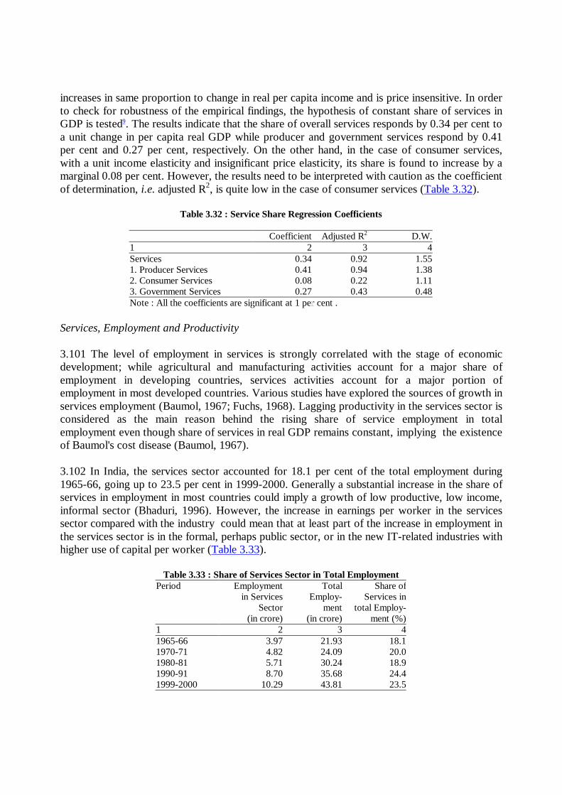
increases in same proportion to change in real per capita income and is price insensitive. In orderto check for robustness of the empirical findings, the hypothesis of constant share of services inGDP is tested9. The results indicate that the share of overall services responds by 0.34 per cent toa unit change in per capita real GDP while producer and government services respond by 0.41per cent and 0.27 per cent, respectively. On the other hand, in the case of consumer services,with a unit income elasticity and insignificant price elasticity, its share is found to increase by amarginal 0.08 per cent. However, the results need to be interpreted with caution as the coefficientof determination, i.e. adjusted R2, is quite low in the case of consumer services (Table 3.32).

Table 3.32 : Service Share Regression Coefficients

Coefficient Adjusted R2 D.W.1 2 3 4Services 0.34 0.92 1.551. Producer Services 0.41 0.94 1.382. Consumer Services 0.08 0.22 1.113. Government Services 0.27 0.43 0.48Note : All the coefficients are significant at 1 per cent .

Services, Employment and Productivity

3.101 The level of employment in services is strongly correlated with the stage of economicdevelopment; while agricultural and manufacturing activities account for a major share ofemployment in developing countries, services activities account for a major portion ofemployment in most developed countries. Various studies have explored the sources of growth inservices employment (Baumol, 1967; Fuchs, 1968). Lagging productivity in the services sector isconsidered as the main reason behind the rising share of service employment in totalemployment even though share of services in real GDP remains constant, implying the existenceof Baumol's cost disease (Baumol, 1967).

3.102 In India, the services sector accounted for 18.1 per cent of the total employment during1965-66, going up to 23.5 per cent in 1999-2000. Generally a substantial increase in the share ofservices in employment in most countries could imply a growth of low productive, low income,informal sector (Bhaduri, 1996). However, the increase in earnings per worker in the servicessector compared with the industry could mean that at least part of the increase in employment inthe services sector is in the formal, perhaps public sector, or in the new IT-related industries withhigher use of capital per worker (Table 3.33).

Table 3.33 : Share of Services Sector in Total EmploymentPeriod Employment Total Share of

in Services Employ- Services inSector ment total Employ-

(in crore) (in crore) ment (%)1 2 3 41965-66 3.97 21.93 18.11970-71 4.82 24.09 20.01980-81 5.71 30.24 18.91990-91 8.70 35.68 24.41999-2000 10.29 43.81 23.5

Source: National Sample Survey Organisation (various rounds)and Visaria,1996.

3.103 In order to focus upon the differences in growth rate of employment and gross value addedin services sector since 1970-71, a difference of means test is employed with the following nullhypotheses: (i) there is no difference in the growth rate of employment in services sector andgrowth rate of gross value added in services sector; (ii) there is no difference between labourproductivity growth and employment growth in services sector. Labour productivity is definedas value added in services sector divided by total labour in services sector (Table 3.34).

Table 3.34 : Difference of Means Test for Differences in Growth Rates

Period Null Hypothesis Mean Finding at 1%difference level of significance

1 2 3 4i) 1970-71 to 1999-2000 No difference between the growth -3.5 Null hypothesis Rejected

rates of Employment and grossvalue added in services sector

ii) 1970-71 to 1999-2000 No difference between the growth rates 0.7 Null hypothesis Acceptedof labour productivity and employmentin services sector

a) 1970-71 to 1979-80 No difference between the growth rates 0.7 Null hypothesis Acceptedof labour productivity and employmentin services sector

b) 1980-81 to 1989-90 No difference between the growth rates -2.2 Null hypothesis Rejectedof labour productivity and employmentin services sector

c) 1990-91 to 1999-2000 No difference between the growth rates 3.6 Null hypothesis Rejectedof labour productivity and employmentin services sector

3. 104 The results show that hypothesis (i) can be rejected, i.e., growth rates of employment andvalue added in services sector are statistically different from each other during 1970-71 to 1999 -2000. As the mean difference is negative, the value added growth in services sector is, on anaverage, higher than employment growth in services sector, which confirms the finding of otherstudies that services sector has undergone a less than proportionate increase in employment inrelation to output (Mitra, 1988; Bhattacharya and Mitra, 1990). The second hypothesis about thedifferences in productivity and employment growth in services has been tested decade-wise.Growth in services productivity for the whole period of 1970-2000 is observed to be higher butnot statistically significant. The growth rate of productivity in services sector has been higherduring the 1990s as the mean difference is found to be positive and statistically significant. Thus,unlike many other countries, growth of average productivity of labour in India has remainedhigher than employment growth in services sector during the post-reform period. The empiricalfindings are supported by the declining capital-output ratio in the services sector which can beinterpreted as efficient use of capital by skilled labour and low contribution of services to totalemployment in contrast to its high contribution to overall GDP. This points towards a growth intotal factor productivity in services (Chart III.45).

Terms-of-Trade

3.105 The services sector is not covered in the construction of Wholesale Price Index (WPI),leaving a major portion of economic activities outside the measurement of headline inflation.Therefore, the inter-sectoral terms-of-trade can only be studied with the help of sectoraldeflators. However, such deflators have their inherent limitations, as they are available with lowfrequency.

3.106 There are divergent views on intersectoral terms-of-trade; nevertheless, the trend insectoral deflators shows that terms-of-trade have remained in favour of agriculture vis-a-visindustry or services all through the 1990s. Thus, the gap between the sectoral deflators has beenwidening in favour of agriculture at the cost of services and industry. On the other hand, acomparison between services and industry shows that terms-of-trade have remained in favour ofservices (Chart III.46).

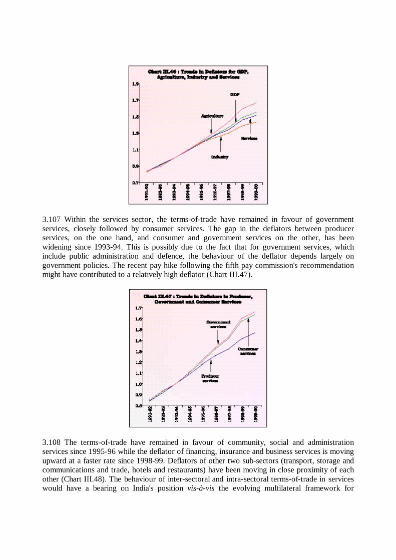
3.107 Within the services sector, the terms-of-trade have remained in favour of governmentservices, closely followed by consumer services. The gap in the deflators between producerservices, on the one hand, and consumer and government services on the other, has beenwidening since 1993-94. This is possibly due to the fact that for government services, whichinclude public administration and defence, the behaviour of the deflator depends largely ongovernment policies. The recent pay hike following the fifth pay commission's recommendationmight have contributed to a relatively high deflator (Chart III.47).

3.108 The terms-of-trade have remained in favour of community, social and administrationservices since 1995-96 while the deflator of financing, insurance and business services is movingupward at a faster rate since 1998-99. Deflators of other two sub-sectors (transport, storage andcommunications and trade, hotels and restaurants) have been moving in close proximity of eachother (Chart III.48). The behaviour of inter-sectoral and intra-sectoral terms-of-trade in serviceswould have a bearing on India's position vis-à-vis the evolving multilateral framework for

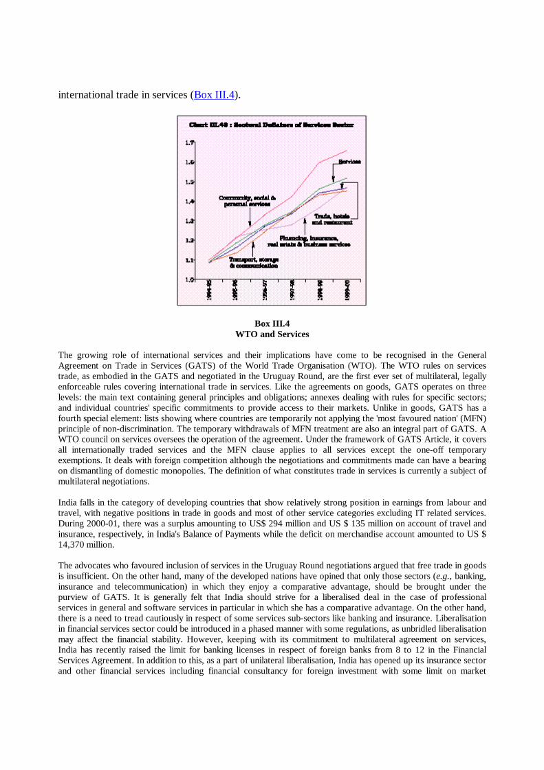
international trade in services (Box III.4).

Box III.4WTO and Services

The growing role of international services and their implications have come to be recognised in the GeneralAgreement on Trade in Services (GATS) of the World Trade Organisation (WTO). The WTO rules on servicestrade, as embodied in the GATS and negotiated in the Uruguay Round, are the first ever set of multilateral, legallyenforceable rules covering international trade in services. Like the agreements on goods, GATS operates on threelevels: the main text containing general principles and obligations; annexes dealing with rules for specific sectors;and individual countries' specific commitments to provide access to their markets. Unlike in goods, GATS has afourth special element: lists showing where countries are temporarily not applying the 'most favoured nation' (MFN)principle of non-discrimination. The temporary withdrawals of MFN treatment are also an integral part of GATS. AWTO council on services oversees the operation of the agreement. Under the framework of GATS Article, it coversall internationally traded services and the MFN clause applies to all services except the one-off temporaryexemptions. It deals with foreign competition although the negotiations and commitments made can have a bearingon dismantling of domestic monopolies. The definition of what constitutes trade in services is currently a subject ofmultilateral negotiations.

India falls in the category of developing countries that show relatively strong position in earnings from labour andtravel, with negative positions in trade in goods and most of other service categories excluding IT related services.During 2000-01, there was a surplus amounting to US$ 294 million and US $ 135 million on account of travel andinsurance, respectively, in India's Balance of Payments while the deficit on merchandise account amounted to US $14,370 million.

The advocates who favoured inclusion of services in the Uruguay Round negotiations argued that free trade in goodsis insufficient. On the other hand, many of the developed nations have opined that only those sectors (e.g., banking,insurance and telecommunication) in which they enjoy a comparative advantage, should be brought under thepurview of GATS. It is generally felt that India should strive for a liberalised deal in the case of professionalservices in general and software services in particular in which she has a comparative advantage. On the other hand,there is a need to tread cautiously in respect of some services sub-sectors like banking and insurance. Liberalisationin financial services sector could be introduced in a phased manner with some regulations, as unbridled liberalisationmay affect the financial stability. However, keeping with its commitment to multilateral agreement on services,India has recently raised the limit for banking licenses in respect of foreign banks from 8 to 12 in the FinancialServices Agreement. In addition to this, as a part of unilateral liberalisation, India has opened up its insurance sectorand other financial services including financial consultancy for foreign investment with some limit on market

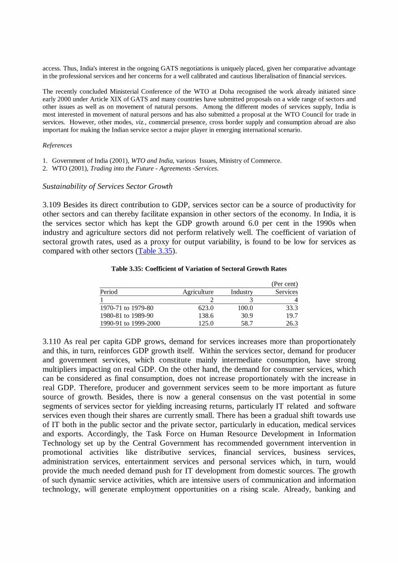
access. Thus, India's interest in the ongoing GATS negotiations is uniquely placed, given her comparative advantagein the professional services and her concerns for a well calibrated and cautious liberalisation of financial services.

The recently concluded Ministerial Conference of the WTO at Doha recognised the work already initiated sinceearly 2000 under Article XIX of GATS and many countries have submitted proposals on a wide range of sectors andother issues as well as on movement of natural persons. Among the different modes of services supply, India ismost interested in movement of natural persons and has also submitted a proposal at the WTO Council for trade inservices. However, other modes, viz., commercial presence, cross border supply and consumption abroad are alsoimportant for making the Indian service sector a major player in emerging international scenario.

References

1. Government of India (2001), WTO and India, various Issues, Ministry of Commerce.2. WTO (2001), Trading into the Future - Agreements -Services.

Sustainability of Services Sector Growth

3.109 Besides its direct contribution to GDP, services sector can be a source of productivity forother sectors and can thereby facilitate expansion in other sectors of the economy. In India, it isthe services sector which has kept the GDP growth around 6.0 per cent in the 1990s whenindustry and agriculture sectors did not perform relatively well. The coefficient of variation ofsectoral growth rates, used as a proxy for output variability, is found to be low for services ascompared with other sectors (Table 3.35).

Table 3.35: Coefficient of Variation of Sectoral Growth Rates

(Per cent)Period Agriculture Industry Services1 2 3 41970-71 to 1979-80 623.0 100.0 33.31980-81 to 1989-90 138.6 30.9 19.71990-91 to 1999-2000 125.0 58.7 26.3

3.110 As real per capita GDP grows, demand for services increases more than proportionatelyand this, in turn, reinforces GDP growth itself. Within the services sector, demand for producerand government services, which constitute mainly intermediate consumption, have strongmultipliers impacting on real GDP. On the other hand, the demand for consumer services, whichcan be considered as final consumption, does not increase proportionately with the increase inreal GDP. Therefore, producer and government services seem to be more important as futuresource of growth. Besides, there is now a general consensus on the vast potential in somesegments of services sector for yielding increasing returns, particularly IT related and softwareservices even though their shares are currently small. There has been a gradual shift towards useof IT both in the public sector and the private sector, particularly in education, medical servicesand exports. Accordingly, the Task Force on Human Resource Development in InformationTechnology set up by the Central Government has recommended government intervention inpromotional activities like distributive services, financial services, business services,administration services, entertainment services and personal services which, in turn, wouldprovide the much needed demand push for IT development from domestic sources. The growthof such dynamic service activities, which are intensive users of communication and informationtechnology, will generate employment opportunities on a rising scale. Already, banking and

insurance sectors have started synergising with IT.

3.111 The financial services sector, with its significant share in services could turn out to be aninfluential source of growth. Export of services which, at present, contributes approximately26.7 per cent of total exports can give a major boost to overall economic growth. Withinformation technology-led global progress, trends are likely to be in favour of a majorexpansion of the world trade in services, particularly communication, financial services,computer and information services, technology transfers and different business services. India,with its large and expanding knowledge base, can explore the opportunities (Raipuria, 2001).The labour productivity in software is twice the ratio of India's manufacturing and 1.3 times thatof the US (Arora and Athreye, 2001). The potential of its high capacity to generate wealth,foreign exchange and employment has been recognised at all levels. The global IT industryoffers Indian companies unique opportunities in four broad areas: value-added IT services,software products, IT enabled services and e-business (Unni and Rani, 2000). As per NASSCOMprojections, India's software and IT services sector is set to grow at a rate of 30 to 35 per centduring 2001-02. The IT industry is slated for a target revenue of US $ 87 billion by 2008 with a7.5 per cent contribution to the GDP.

3.112 The process of economic growth has itself led to the emergence and expansion of newservices such as advertising, publicity, marketing, etc. These sub-sectors provide essentialservice inputs to other sectors in the economy, thereby developing strong linkages with the restof economy. Various studies have examined the expansionary potential of services sector innon-services industries and found strong forward linkages, as 50 per cent of the industries in theeconomy are found to be directly or indirectly service intensive (Dutta, 1989; Bhowmik, 2000).

3.113 Efficient delivery of services increases the productivity of both labour and capital in theeconomy as a whole. In general, services sector appears to be highly growth inducing withpositive externalities for other sectors, making services a catalytic agent of growth. It needs to berecognised that the services sector in itself is not homogenous. Therefore, the expansion of thesesectors needs to be calibrated and integrated simultaneously into the overall growth process toimpart an element of sustainability.

V. REGIONAL DIMENSION OF ECONOMIC GROWTH IN INDIA

3.114 The regional dimensions of growth of the Indian economy are assuming increasingrelevance in the context of the progressive diffusion of structural reforms at the sub-nationallevel. The quality of growth is getting increasingly assessed in terms of durable improvement inthe regional growth profiles in which the interface between public policies for acceleratingdevelopment and standards of living is the greatest. Moreover, regional patterns of growthprovide a gauge of the quality of public policies themselves and their impact on macroeconomicwelfare. The various facets of the growth experience of States in India are critical for developingan understanding of the sources of demand generation as well as changes in productivity andgrowth. The growth performance in the States is often the outcome of institutional and non-economic factors interacting with the initial conditions which encompass various aspects ofhuman capital development.

3.115 Varying degrees of reform in different States have yielded wide variations in growthperformance. In this context, it has been pointed out that the popular characterisation ofbackward States such as Bihar, Madhya Pradesh (M.P.), Rajasthan, and Uttar Pradesh (U.P.) as ahomogenous group of poor performers does not hold good in terms of recent economicperformance (Ahluwalia, 2000). It has also been argued that reforms have unshackled a numberof States like Andhra Pradesh (A.P.), Gujarat, Karnataka, Maharashtra and Tamil Nadu (T.N.)who could achieve their true economic potential in recent years (Bajpai and Sachs, 1999). Froma completely different paradigm, the faster growth in select States has been interpreted as theoperation of some kind of unbalanced growth with differing rates of catching up (Chaudhuri,2000). Three other issues are raised in the context of Indian regional development, viz., fiscal,infrastructure and human resources development (World Bank, 2000).

Regional Growth Profiles10

3.116 The State-wise profile of per capita State Domestic Product (SDP) drawn up for 15 majorStates (representing nearly 90 per cent of Indian population) exhibits significant variation. In1980-81, there were only four States viz., Maharashtra, Punjab, Gujarat and Haryana whose percapita real SDPs (at 1980-81 prices) were higher than the all-India per capita real GDP (Table3.36). The trend remained more or less similar in 1990-91. In the 1990s, this group expanded toinclude Tamil Nadu. Relative rankings in terms of absolute SDP need to be evaluated against acomparison of growth rates. In terms of trend growth rate, Karnataka, West Bengal, Maharashtra,Tamil Nadu, Andhra Pradesh have done well in the 1990s (Chart III.49).

Table 3.36 : Trend Growth Rate of Per Capita SDP(Per cent)

1980-81 = 100 1993-94 =100States 1981-82 to 1981-82 to 1993-94 to

1990-91 1993-94 1999-20001 2 3 4

1 Karnataka 4.0 4.5 4.52 Gujarat 3.3 3.1 2.43 West Bengal 2.7 2.9 5.6

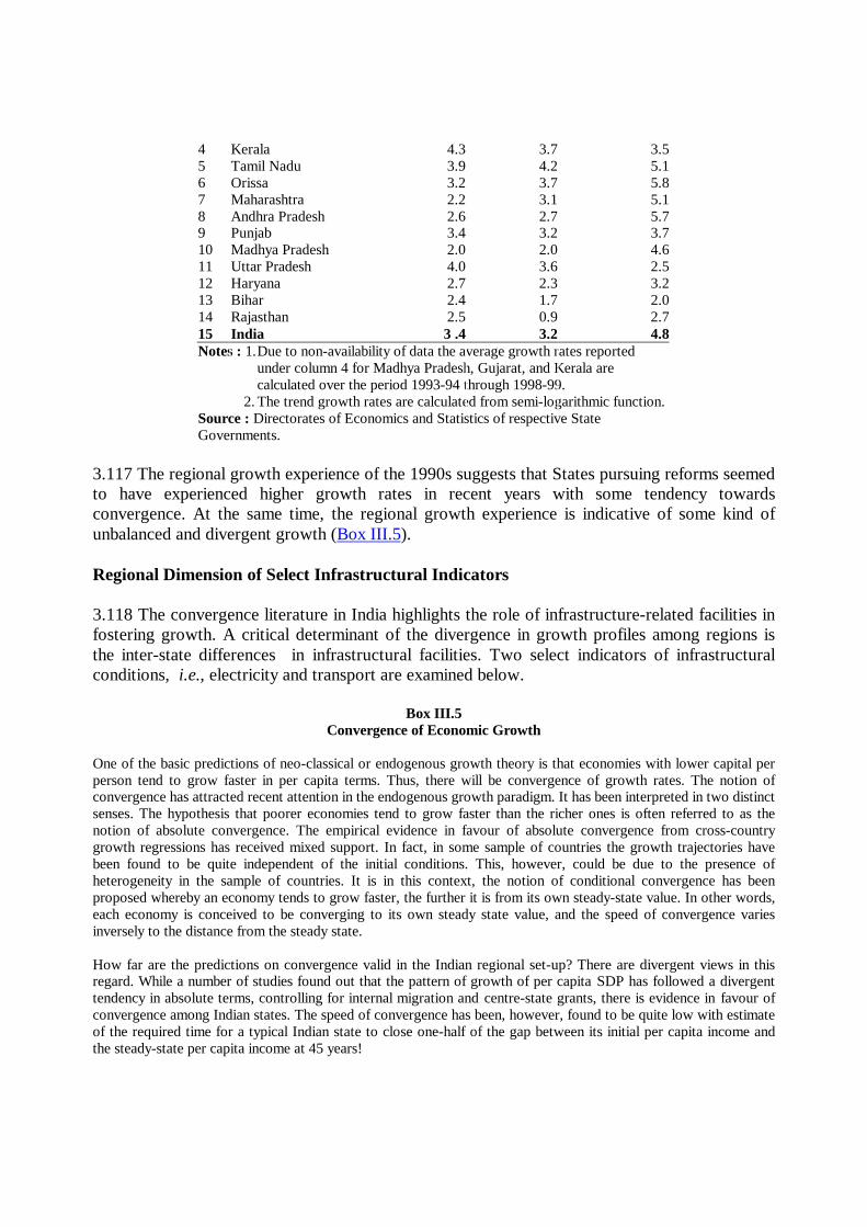
4 Kerala 4.3 3.7 3.55 Tamil Nadu 3.9 4.2 5.16 Orissa 3.2 3.7 5.87 Maharashtra 2.2 3.1 5.18 Andhra Pradesh 2.6 2.7 5.79 Punjab 3.4 3.2 3.710 Madhya Pradesh 2.0 2.0 4.611 Uttar Pradesh 4.0 3.6 2.512 Haryana 2.7 2.3 3.213 Bihar 2.4 1.7 2.014 Rajasthan 2.5 0.9 2.715 India 3 .4 3.2 4.8Notes : 1.Due to non-availability of data the average growth rates reported

under column 4 for Madhya Pradesh, Gujarat, and Kerala arecalculated over the period 1993-94 through 1998-99.

2. The trend growth rates are calculated from semi-logarithmic function.Source : Directorates of Economics and Statistics of respective StateGovernments.

3.117 The regional growth experience of the 1990s suggests that States pursuing reforms seemedto have experienced higher growth rates in recent years with some tendency towardsconvergence. At the same time, the regional growth experience is indicative of some kind ofunbalanced and divergent growth (Box III.5).

Regional Dimension of Select Infrastructural Indicators

3.118 The convergence literature in India highlights the role of infrastructure-related facilities infostering growth. A critical determinant of the divergence in growth profiles among regions isthe inter-state differences in infrastructural facilities. Two select indicators of infrastructuralconditions, i.e., electricity and transport are examined below.

Box III.5Convergence of Economic Growth

One of the basic predictions of neo-classical or endogenous growth theory is that economies with lower capital perperson tend to grow faster in per capita terms. Thus, there will be convergence of growth rates. The notion ofconvergence has attracted recent attention in the endogenous growth paradigm. It has been interpreted in two distinctsenses. The hypothesis that poorer economies tend to grow faster than the richer ones is often referred to as thenotion of absolute convergence. The empirical evidence in favour of absolute convergence from cross-countrygrowth regressions has received mixed support. In fact, in some sample of countries the growth trajectories havebeen found to be quite independent of the initial conditions. This, however, could be due to the presence ofheterogeneity in the sample of countries. It is in this context, the notion of conditional convergence has beenproposed whereby an economy tends to grow faster, the further it is from its own steady-state value. In other words,each economy is conceived to be converging to its own steady state value, and the speed of convergence variesinversely to the distance from the steady state.

How far are the predictions on convergence valid in the Indian regional set-up? There are divergent views in thisregard. While a number of studies found out that the pattern of growth of per capita SDP has followed a divergenttendency in absolute terms, controlling for internal migration and centre-state grants, there is evidence in favour ofconvergence among Indian states. The speed of convergence has been, however, found to be quite low with estimateof the required time for a typical Indian state to close one-half of the gap between its initial per capita income andthe steady-state per capita income at 45 years!

What explains the pattern and extent of divergence among the growth profiles of Indian states, if any? Incorporationof omitted variables in the growth regression across Indian states has attracted attention in recent years. In thedetermination of regional steady-state level of income and ensuring conditional convergence, a number of variableshave been highlighted, viz., literacy and per capita investment. In fact, it has been hypothesised that states withhigher levels of income can undertake more ambitious infrastructure investment programmes, since they enjoy morefiscal revenues to pay from it. A contrary view regarding diverging tendency of per capita SDP growth is found aswell. A number of reasons for such diverging trends has been cited, viz., (a) differences in private investment andpublic expenditure, (b) differing distribution of state Government expenditure, (c) regressivity of implicit inter-governmental transfers, (d) lack of horizontal equity in inter-governmental transfers, and (e) regional policies.

In the ultimate analysis, while much of the evidence of growth differentials among Indian states hints at someoperation of conditional convergence, the determination of steady-state growth rate for a State is by itself a seriouspolicy question. Thus, any explanation for convergence of (or its lack) growth across Indian States needs to besought in the interplay of all these control variables, perhaps along with the institutional set-up prevalent in theregion.

References:

1. Aiyar, Shekhar, 2000, "Growth Theory and Convergence across Indian States: A Panel Study", in Callen, Tim,Patricia Reynolds, and Christopher Towe (eds.). India at the Crossroads: Sustaining Growth and ReducingPoverty, International Monetary Fund, Washington DC.

2. Barro, R.J. and X. Sala-i-Martin,1992, "Convergence", Journal of Political Economy, Vol. 100.3. Cashin, P. and R. Sahay, 1996, "Internal Migration, Centre-State Grants and Economic Growth in the States of

India", IMF Staff Papers, Vol. 43.4. Marjit, S. and S. Mitra, 1996, "Convergence in Regional Growth Rates: Indian Research Agenda", Economic

and Political Weekly, August 17.5. Nagaraj, R., A. Varoudakis, and M. A. Veganzones, 2000, "Long-Run Growth Trends and Convergence across

Indian States", Journal of International Development, Vol. 12.6. Rao, M Govinda, R.T Shand, and K.P.Kalirajan, 1999, "Convergence of Income across Indian States: A

Divergent View", Economic and Political Weekly, March 27.

Power Supply

3.119 Electricity occupies a critical role in infrastructure. Various factors determine the demandand supply of this crucial input. The level of industrialisation, urbanisation, user cost and tariffstructure, presence of subsidies, all could play a significant role in the determination of demand;on the other hand, technological and institutional arrangements are the crucial factors influencingsupply. The electricity sector in various States suffer from endemic problems - unviable StateElectricity Boards (SEBs), transmission losses and distortive subsidy structure. The relationshipbetween the power situation and the regional growth in the 1990s reveals that there has been ageneral improvement in the power supply position in all the States in terms of deficit (i.e.,requirement less availability as a percentage of requirement). In fact, two States viz., Orissa andWest Bengal have managed to transform their power position from deficit to surplus (Table3.37).

3.120 The existence of surplus power is, however, no indication of well being in the electricitysector. Out of the five States with deficits higher than the all-India average, three States, viz.,Karnataka, Gujarat, and Maharashtra were high growth States in the 1990s.

Table 3.37 : State-wise Power Supply Position(in MUs)

State 1991-92 2000-01

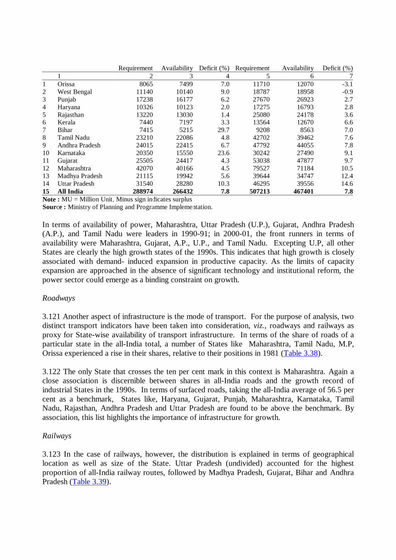
Requirement Availability Deficit (%) Requirement Availability Deficit (%)1 2 3 4 5 6 7

1 Orissa 8065 7499 7.0 11710 12070 -3.12 West Bengal 11140 10140 9.0 18787 18958 -0.93 Punjab 17238 16177 6.2 27670 26923 2.74 Haryana 10326 10123 2.0 17275 16793 2.85 Rajasthan 13220 13030 1.4 25080 24178 3.66 Kerala 7440 7197 3.3 13564 12670 6.67 Bihar 7415 5215 29.7 9208 8563 7.08 Tamil Nadu 23210 22086 4.8 42702 39462 7.69 Andhra Pradesh 24015 22415 6.7 47792 44055 7.810 Karnataka 20350 15550 23.6 30242 27490 9.111 Gujarat 25505 24417 4.3 53038 47877 9.712 Maharashtra 42070 40166 4.5 79527 71184 10.513 Madhya Pradesh 21115 19942 5.6 39644 34747 12.414 Uttar Pradesh 31540 28280 10.3 46295 39556 14.615 All India 288974 266432 7.8 507213 467401 7.8Note : MU = Million Unit, Minus sign indicates surplusSource : Ministry of Planning and Programme Implementation.

In terms of availability of power, Maharashtra, Uttar Pradesh (U.P.), Gujarat, Andhra Pradesh(A.P.), and Tamil Nadu were leaders in 1990-91; in 2000-01, the front runners in terms ofavailability were Maharashtra, Gujarat, A.P., U.P., and Tamil Nadu. Excepting U.P, all otherStates are clearly the high growth states of the 1990s. This indicates that high growth is closelyassociated with demand- induced expansion in productive capacity. As the limits of capacityexpansion are approached in the absence of significant technology and institutional reform, thepower sector could emerge as a binding constraint on growth.

Roadways

3.121 Another aspect of infrastructure is the mode of transport. For the purpose of analysis, twodistinct transport indicators have been taken into consideration, viz., roadways and railways asproxy for State-wise availability of transport infrastructure. In terms of the share of roads of aparticular state in the all-India total, a number of States like Maharashtra, Tamil Nadu, M.P,Orissa experienced a rise in their shares, relative to their positions in 1981 (Table 3.38).

3.122 The only State that crosses the ten per cent mark in this context is Maharashtra. Again aclose association is discernible between shares in all-India roads and the growth record ofindustrial States in the 1990s. In terms of surfaced roads, taking the all-India average of 56.5 percent as a benchmark, States like, Haryana, Gujarat, Punjab, Maharashtra, Karnataka, TamilNadu, Rajasthan, Andhra Pradesh and Uttar Pradesh are found to be above the benchmark. Byassociation, this list highlights the importance of infrastructure for growth.

Railways

3.123 In the case of railways, however, the distribution is explained in terms of geographicallocation as well as size of the State. Uttar Pradesh (undivided) accounted for the highestproportion of all-India railway routes, followed by Madhya Pradesh, Gujarat, Bihar and AndhraPradesh (Table 3.39).

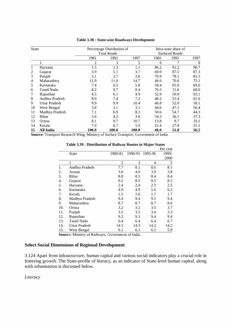
Table 3.38 : State-wise Roadways Development

State Percentage Distribution of Intra-state share ofTotal Roads Surfaced Roads

1981 1991 1997 1981 1991 19971 2 3 5 6 7 8

1 Haryana 1.5 1.3 1.1 86.2 91.2 90.72 Gujarat 3.9 5.1 3.7 69.9 87.5 87.33 Punjab 3.1 2.7 2.6 76.9 78.1 81.54 Maharashtra 11.9 11.0 14.7 46.0 70.6 75.15 Karnataka 7.4 6.5 5.8 58.4 65.0 69.06 Tamil Nadu 8.2 9.7 8.4 76.5 15.6 68.07 Rajasthan 4.5 6.1 4.9 52.9 50.9 63.18 Andhra Pradesh 8.0 7.4 7.2 48.2 53.4 61.69 Uttar Pradesh 9.9 9.9 10.4 46.8 52.0 58.110 West Bengal 3.8 3.1 3.1 44.6 47.1 56.411 Madhya Pradesh 7.1 6.9 8.1 50.6 54.7 44.312 Bihar 5.6 4.2 3.6 34.3 36.1 37.313 Orissa 8.1 9.7 10.7 13.8 9.7 33.114 Kerala 7.0 6.7 5.9 22.4 27.8 31.115 All India 100.0 100.0 100.0 46.0 51.8 56.5Source: Transport Research Wing, Ministry of Surface Transport, Government of India.

Table 3.39 : Distribution of Railway Routes in Major StatesPer cent

State 1980-81 1990-91 1995-96 1999-2000

1 2 3 4 51. Andhra Pradesh 7.7 8.1 8.0 8.12. Assam 3.6 4.0 3.9 3.83. Bihar 8.8 8.5 8.4 8.44. Gujarat 9.2 8.5 8.5 8.55. Haryana 2.4 2.4 2.3 2.56. Karnataka 4.9 4.9 5.0 6.37. Kerala 1.5 1.6 1.7 1.78. Madhya Pradesh 9.4 9.4 9.5 9.49. Maharashtra 8.7 8.7 8.7 8.610. Orissa 3.2 3.2 3.5 3.711. Punjab 3.5 3.5 3.4 3.312. Rajasthan 9.2 9.3 9.4 9.413. Tamil Nadu 6.4 6.4 6.4 6.714. Uttar Pradesh 14.5 14.3 14.2 14.215. West Bengal 6.1 6.1 6.1 5.9Source: Ministry of Railways, Government of India.

Select Social Dimensions of Regional Development

3.124 Apart from infrastructure, human capital and various social indicators play a crucial role infostering growth. The State-profile of literacy, as an indicator of State-level human capital, alongwith urbanisation is discussed below.

Literacy

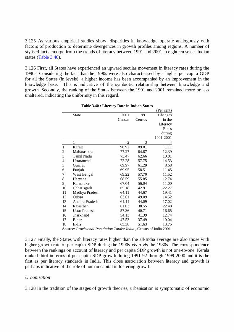
3.125 As various empirical studies show, disparities in knowledge operate analogously withfactors of production to determine divergences in growth profiles among regions. A number ofstylised facts emerge from the trends of literacy between 1991 and 2001 in eighteen select Indianstates (Table 3.40).

3.126 First, all States have experienced an upward secular movement in literacy rates during the1990s. Considering the fact that the 1990s were also characterised by a higher per capita GDPfor all the States (in levels), a higher income has been accompanied by an improvement in theknowledge base. This is indicative of the symbiotic relationship between knowledge andgrowth. Secondly, the ranking of the States between the 1991 and 2001 remained more or lessunaltered, indicating the uniformity in this regard.

Table 3.40 : Literacy Rate in Indian States(Per cent)

State 2001 1991 ChangesCensus Census in the

LiteracyRates

during1991-2001

1 2 3 41 Kerala 90.92 89.81 1.112 Maharashtra 77.27 64.87 12.393 Tamil Nadu 73.47 62.66 10.814 Uttaranchal 72.28 57.75 14.535 Gujarat 69.97 61.29 8.686 Punjab 69.95 58.51 11.457 West Bengal 69.22 57.70 11.528 Haryana 68.59 55.85 12.749 Karnataka 67.04 56.04 11.0010 Chhatisgarh 65.18 42.91 22.2711 Madhya Pradesh 64.11 44.67 19.4112 Orissa 63.61 49.09 14.5213 Andhra Pradesh 61.11 44.09 17.0214 Rajasthan 61.03 38.55 22.4815 Uttar Pradesh 57.36 40.71 16.6516 Jharkhand 54.13 41.39 12.7417 Bihar 47.53 37.49 10.0418 India 65.38 51.63 13.75Source: Provisional Population Totals: India , Census of India 2001.

3.127 Finally, the States with literacy rates higher than the all-India average are also those withhigher growth rate of per capita SDP during the 1990s vis-a-vis the 1980s. The correspondencebetween the rankings on account of literacy and per capita SDP growth is not one-to-one. Keralaranked third in terms of per capita SDP growth during 1991-92 through 1999-2000 and it is thefirst as per literacy standards in India. This close association between literacy and growth isperhaps indicative of the role of human capital in fostering growth.

Urbanisation

3.128 In the tradition of the stages of growth theories, urbanisation is symptomatic of economic

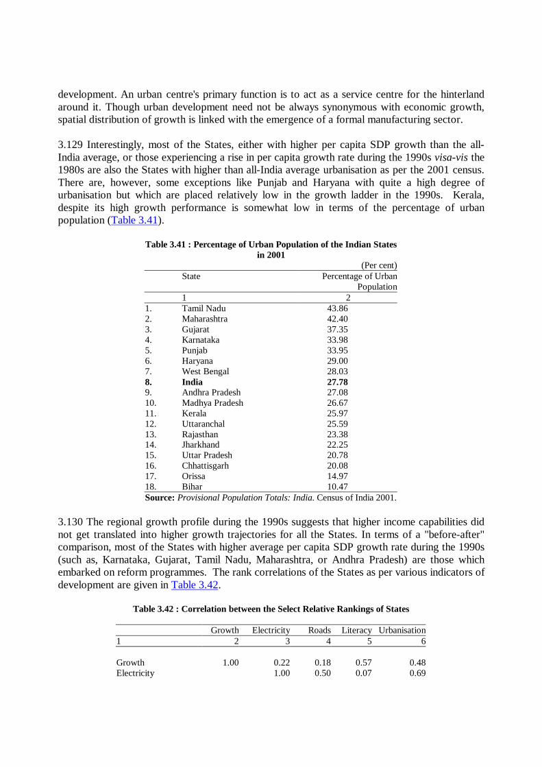
development. An urban centre's primary function is to act as a service centre for the hinterlandaround it. Though urban development need not be always synonymous with economic growth,spatial distribution of growth is linked with the emergence of a formal manufacturing sector.

3.129 Interestingly, most of the States, either with higher per capita SDP growth than the all-India average, or those experiencing a rise in per capita growth rate during the 1990s visa-vis the1980s are also the States with higher than all-India average urbanisation as per the 2001 census.There are, however, some exceptions like Punjab and Haryana with quite a high degree ofurbanisation but which are placed relatively low in the growth ladder in the 1990s. Kerala,despite its high growth performance is somewhat low in terms of the percentage of urbanpopulation (Table 3.41).

Table 3.41 : Percentage of Urban Population of the Indian Statesin 2001

(Per cent)State Percentage of Urban

Population1 2

1. Tamil Nadu 43.862. Maharashtra 42.403. Gujarat 37.354. Karnataka 33.985. Punjab 33.956. Haryana 29.007. West Bengal 28.038. India 27.789. Andhra Pradesh 27.0810. Madhya Pradesh 26.6711. Kerala 25.9712. Uttaranchal 25.5913. Rajasthan 23.3814. Jharkhand 22.2515. Uttar Pradesh 20.7816. Chhattisgarh 20.0817. Orissa 14.9718. Bihar 10.47Source: Provisional Population Totals: India. Census of India 2001.

3.130 The regional growth profile during the 1990s suggests that higher income capabilities didnot get translated into higher growth trajectories for all the States. In terms of a "before-after"comparison, most of the States with higher average per capita SDP growth rate during the 1990s(such as, Karnataka, Gujarat, Tamil Nadu, Maharashtra, or Andhra Pradesh) are those whichembarked on reform programmes. The rank correlations of the States as per various indicators ofdevelopment are given in Table 3.42.

Table 3.42 : Correlation between the Select Relative Rankings of States

Growth Electricity Roads Literacy Urbanisation1 2 3 4 5 6

Growth 1.00 0.22 0.18 0.57 0.48Electricity 1.00 0.50 0.07 0.69

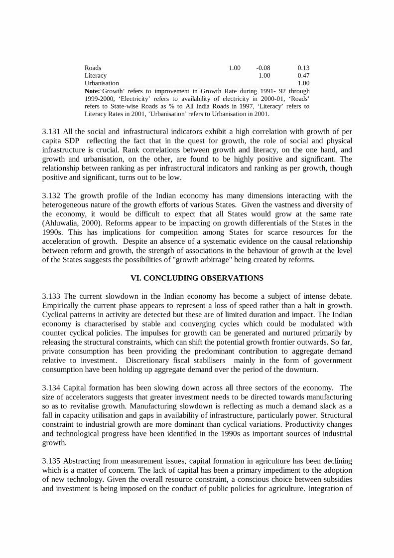
Roads 1.00 -0.08 0.13Literacy 1.00 0.47Urbanisation 1.00Note:‘Growth’ refers to improvement in Growth Rate during 1991- 92 through1999-2000, ‘Electricity’ refers to availability of electricity in 2000-01, ‘Roads’refers to State-wise Roads as % to All India Roads in 1997, ‘Literacy’ refers toLiteracy Rates in 2001, ‘Urbanisation’ refers to Urbanisation in 2001.

3.131 All the social and infrastructural indicators exhibit a high correlation with growth of percapita SDP reflecting the fact that in the quest for growth, the role of social and physicalinfrastructure is crucial. Rank correlations between growth and literacy, on the one hand, andgrowth and urbanisation, on the other, are found to be highly positive and significant. Therelationship between ranking as per infrastructural indicators and ranking as per growth, thoughpositive and significant, turns out to be low.

3.132 The growth profile of the Indian economy has many dimensions interacting with theheterogeneous nature of the growth efforts of various States. Given the vastness and diversity ofthe economy, it would be difficult to expect that all States would grow at the same rate(Ahluwalia, 2000). Reforms appear to be impacting on growth differentials of the States in the1990s. This has implications for competition among States for scarce resources for theacceleration of growth. Despite an absence of a systematic evidence on the causal relationshipbetween reform and growth, the strength of associations in the behaviour of growth at the levelof the States suggests the possibilities of "growth arbitrage" being created by reforms.

VI. CONCLUDING OBSERVATIONS

3.133 The current slowdown in the Indian economy has become a subject of intense debate.Empirically the current phase appears to represent a loss of speed rather than a halt in growth.Cyclical patterns in activity are detected but these are of limited duration and impact. The Indianeconomy is characterised by stable and converging cycles which could be modulated withcounter cyclical policies. The impulses for growth can be generated and nurtured primarily byreleasing the structural constraints, which can shift the potential growth frontier outwards. So far,private consumption has been providing the predominant contribution to aggregate demandrelative to investment. Discretionary fiscal stabilisers mainly in the form of governmentconsumption have been holding up aggregate demand over the period of the downturn.

3.134 Capital formation has been slowing down across all three sectors of the economy. Thesize of accelerators suggests that greater investment needs to be directed towards manufacturingso as to revitalise growth. Manufacturing slowdown is reflecting as much a demand slack as afall in capacity utilisation and gaps in availability of infrastructure, particularly power. Structuralconstraint to industrial growth are more dominant than cyclical variations. Productivity changesand technological progress have been identified in the 1990s as important sources of industrialgrowth.

3.135 Abstracting from measurement issues, capital formation in agriculture has been decliningwhich is a matter of concern. The lack of capital has been a primary impediment to the adoptionof new technology. Given the overall resource constraint, a conscious choice between subsidiesand investment is being imposed on the conduct of public policies for agriculture. Integration of

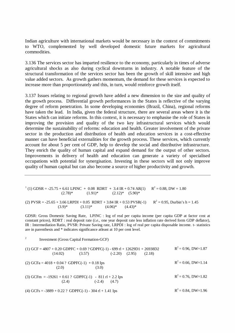
Indian agriculture with international markets would be necessary in the context of commitmentsto WTO, complemented by well developed domestic future markets for agriculturalcommodities.

3.136 The services sector has imparted resilience to the economy, particularly in times of adverseagricultural shocks as also during cyclical downturns in industry. A notable feature of thestructural transformation of the services sector has been the growth of skill intensive and highvalue added sectors. As growth gathers momentum, the demand for these services is expected toincrease more than proportionately and this, in turn, would reinforce growth itself.

3.137 Issues relating to regional growth have added a new dimension to the size and quality ofthe growth process. Differential growth performances in the States is reflective of the varyingdegree of reform penetration. In some developing economies (Brazil, China), regional reformshave taken the lead. In India, given the federal structure, there are several areas where it is theStates which can initiate reforms. In this context, it is necessary to emphasise the role of States inimproving the provision and quality of the two key infrastructural services which woulddetermine the sustainability of reforms: education and health. Greater involvement of the privatesector in the production and distribution of health and education services in a cost-effectivemanner can have beneficial externalities for the growth process. These services, which currentlyaccount for about 5 per cent of GDP, help to develop the social and distributive infrastructure.They enrich the quality of human capital and expand demand for the output of other sectors.Improvements in delivery of health and education can generate a variety of specialisedoccupations with potential for synergisation. Investing in these sectors will not only improvequality of human capital but can also become a source of higher productivity and growth.

1 (1) GDSR = -25.75 + 6.61 LPINC + 0.08 RDRT + 3.4 IR + 0.74 AR(1) R2 = 0.88, DW = 1.80(2.78)* (1.91)* (2.12)* (5.90)*

(2) PVSR = -25.65 + 3.66 LRPDI + 0.05 RDRT + 3.84 IR + 0.53 PVSR(-1) R2 = 0.95, Durbin’s h = 1.45(3.9)* (3.11)* (4.06)* (4.43)*

GDSR: Gross Domestic Saving Rate, LPINC : log of real per capita income (per capita GDP at factor cost atconstant prices), RDRT : real deposit rate (i.e., one year deposit rate less inflation rate derived form GDP deflator),IR : Intermediation Ratio, PVSR: Private Saving rate, LRPDI : log of real per capita disposable income. t- statisticsare in parenthesis and * indicates significance atleast at 10 per cent level.

2 Investment (Gross Capital Formation-GCF)

(1) GCF = 4807 + 0.20 GDPFC + 0.69 ? GDPFC(-1) - 699 rl + 12629D1 + 26938D2 R2 = 0.96, DW=1.87(14.02) (3.57) (-2.20) (2.95) (2.18)

(2) GCFa = 4018 + 0.04 ? GDPFC(-1) + 0.18 Ips R2 = 0.66, DW=1.14(2.0) (3.0)

(3) GCFm = -19261 + 0.61 ? GDPFC(-1) - 811 rl + 2.2 Ips R2 = 0.76, DW=1.82(2.4) (-2.4) (4.7)

(4) GCFs = -3889 + 0.22 ? GDPFC(-1) - 304 rl + 1.41 Ips R2 = 0.84, DW=1.96

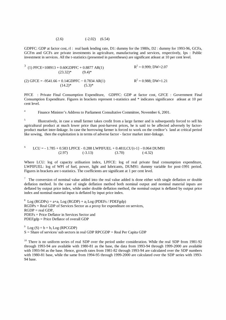
(2.6) (-2.02) (6.54)

GDPFC: GDP at factor cost, rl : real bank lending rate, D1: dummy for the 1980s, D2 : dummy for 1993-96, GCFa,GCFm and GCFs are private investments in agriculture, manufacturing and services, respectively, Ips : Publicinvestment in services. All the t-statistics (presented in parentheses) are significant atleast at 10 per cent level.

3 (1) PFCE=108913 + 0.60GDPFC + 0.8877 AR(1) R2 = 0.999; DW=2.07(23.32)* (9.4)*

(2) GFCE = -9541.66 + 0.14GDPFC + 0.7834 AR(1) R2 = 0.988; DW=1.21(14.2)* (5.3)*

PFCE : Private Final Consumption Expenditure, GDPFC: GDP at factor cost, GFCE : Government FinalConsumption Expenditure. Figures in brackets represent t-statistics and * indicates significance atleast at 10 percent level.

4 Finance Minister’s Address to Parliament Consultative Committee, November 6, 2001.

5 Illustratively, in case a small farmer takes credit from a large farmer and is subsequently forced to sell hisagricultural product at much lower price than post-harvest prices, he is said to be affected adversely by factor-product market inter-linkage. In case the borrowing farmer is forced to work on the creditor’s land at critical periodlike sowing, then the exploitation is in terms of adverse factor - factor market inter-linkage.

6 LCU = - 1.785 + 0.583 LPFCE - 0.288 LWPIFUEL + 0.481LCU{t-1} - 0.064 DUM91(2.97) (-3.13) (3.70) (-4.32)

Where LCU: log of capacity utilisation index, LPFCE: log of real private final consumption expenditure,LWPIFUEL: log of WPI of fuel, power, light and lubricants, DUM91: dummy variable for post-1991 period.Figures in brackets are t-statistics. The coefficients are significant at 1 per cent level.

7 The conversion of nominal value added into the real value added is done either with single deflation or doubledeflation method. In the case of single deflation method both nominal output and nominal material inputs aredeflated by output price index, while under double deflation method, the nominal output is deflated by output priceindex and nominal material input is deflated by input price index.

8 Log (RGDPs) = a+a1 Log (RGDP) + a2 Log (PDEFs / PDEFgdp)RGDPs = Real GDP of Services Sector as a proxy for expenditure on services,RGDP = real GDP,PDEFs = Price Deflator in Services Sector andPDEFgdp = Price Deflator of overall GDP

9 Log (S) = b + b1 Log (RPCGDP)S = Share of services/ sub sectors in real GDP RPCGDP = Real Per Capita GDP

10 There is no uniform series of real SDP over the period under consideration. While the real SDP from 1981-92through 1993-94 are available with 1980-81 as the base, the data from 1993-94 through 1999-2000 are availablewith 1993-94 as the base. Hence, growth rates from 1981-82 through 1993-94 are calculated over the SDP numberswith 1980-81 base, while the same from 1994-95 through 1999-2000 are calculated over the SDP series with 1993-94 base.