1

Image Analysis and Morphometry

Lukas Schärer

Evolutionary Biology

Zoological Institute

University of Basel

13. /15.3.2013 Zoology & Evolution Block Course

2

• Quantifying morphology• why do we need it?

• Image acquisition• image formats and lighting conditions

• Particle analysis• determining particle size with ImageJ

• statistical analysis with JMP

• Geometric morphometrics• analysis of complex shape variation

• placing landmarks with tpsDig

• relative warp analysis with tpsRelw

• statistical analysis with JMP

Summary

3

• phenotypic differences between individuals in a population are the combined result of genetic variation, environmental influences during development and usage of the structure

• natural selection acts on differences in the phenotype between individuals

• so a quantitative understanding of phenotypic variation is required to understand development and evolution

• many traits can be measured directly from the individuals, e.g. using a caliper

• but computer assisted image analysis can often help to quantify more complex traits and it can greatly speed up analysis

Quantifying morphology

4

• precision and accuracy are two different issues• one can measure something with very little measurement error, but still have a

biased sample

Quantifying morphology

from Howard & Read 1998

5

• an image is a table of numbers and each cell in represents one pixel

• cell values range from 0-255 (i.e. 8-bits) with white 0 and black 255 (or vice versa) and many shades of grey in between

• for some image analyses it is better to have 16-bits per pixel (65536 grey levels)

Image acquisition

1 2 3 4

1 0 255 127 63

2 0 5 255 255

3 31 31 31 31

4 15 191 250 255

x-coordinate

y-co

ordi

nate

1 2 3 4

1

2

3

4

x-coordinate

y-co

ordi

nate

6

• it is therefore possible to make calculations with images• one can, for example, add, subtract or average two images

• one can select all the values above or below a certain threshold

pixel! grey-level 0! 951! 962! 963! 964! 955! 956! 957! 958! 959! 9510! 9411! 9312! 9313! 9214! 9115! 8916! 83

pixel! grey-level 17! 7318! 6119! 5220! 4721! 4622! 4723! 4824! 5025! 5226! 5327! 5428! 5529! 5630! 5731! 5832! 59

Image acquisition

7

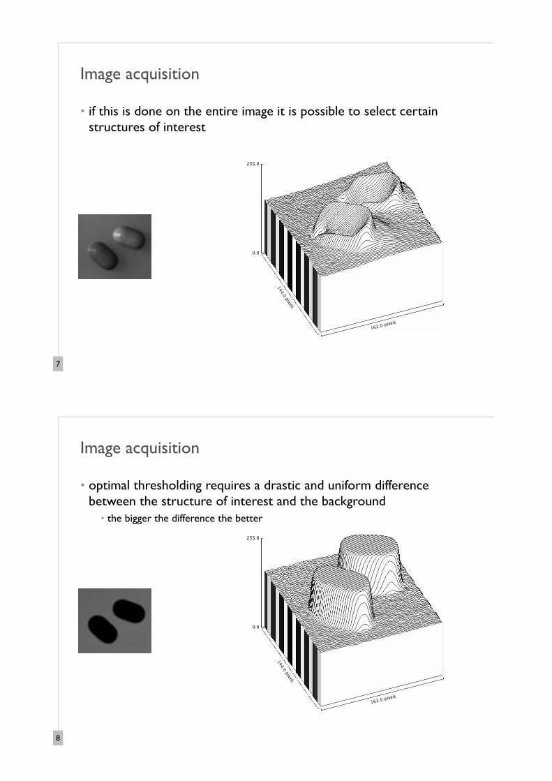
• if this is done on the entire image it is possible to select certain structures of interest

Image acquisition

8

• optimal thresholding requires a drastic and uniform difference between the structure of interest and the background

• the bigger the difference the better

Image acquisition

9

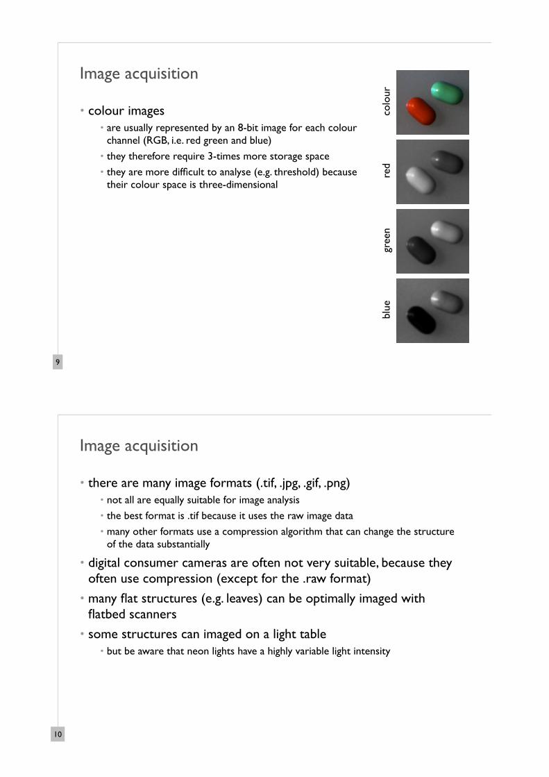
• colour images• are usually represented by an 8-bit image for each colour

channel (RGB, i.e. red green and blue)

• they therefore require 3-times more storage space

• they are more difficult to analyse (e.g. threshold) because their colour space is three-dimensional

colo

urgr

een

blue

red

Image acquisition

10

• there are many image formats (.tif, .jpg, .gif, .png)• not all are equally suitable for image analysis

• the best format is .tif because it uses the raw image data

• many other formats use a compression algorithm that can change the structure of the data substantially

• digital consumer cameras are often not very suitable, because they often use compression (except for the .raw format)

• many flat structures (e.g. leaves) can be optimally imaged with flatbed scanners

• some structures can imaged on a light table• but be aware that neon lights have a highly variable light intensity

Image acquisition

11

• many morphological characters are particulate• so they have a distribution, an average size and a variance

(see e.g., the fish eggs, red blood cells or virus particles depicted on the right)

• to estimate these measures requires measuring many particles per individual

Particle analysis

12

• open file in ImageJ

• select the line tool and measure a known distance on the ruler (e.g. 10 cm)• measuring a long distance reduces the error

• choose Analyse > Set Scale and enter the distance in the field ‘known distance’• check the box Global (so future images are opened with same calibration)

• choose Image > Type > 8-bit (to remove the colour information)

• select the area with the particles using the rectangle tool and then select Image > Duplicate (this makes a new file with only the particles)

• choose Image > Adjust > Threshold and set the upper and lower thresholds to select the particles

• click on the Apply button to convert the image into a bitmap (1-bit per pixel)

• select a small particle using the wand tool, measure it (Analyze > Measure), check the results and then deselect it using (Edit > Selection > Select None)

• choose Analyze > Analyze Particles and set the size range to include the smallest particles (this allows to ignore dirt or other things)

Particle analysis: a worked example

13

• copy the results table and paste it into JMP

• check the size distribution of the particles by choosing Analyze > Distribution• look at the distribution and the values that are reported• what do you observe? is the distribution unimodal? is it a normal

distribution? could it be that there are different types of TicTac?

• classify the TicTac according to type and compare them by choosing Analyze > Fit Y by X

• choose type as the X variable and particle area as the Y variable• select Means/ANOVA/Pooled t and Means and Std Dev from red arrow

menu• look at the figure, the different measures of central tendency and the

statistics that are reported

• make a conclusion

Particle analysis: a worked example

14

• the aim of geometric morphometrics is the analysis of complex shape variation

• shape variation can be analysed by measuring the linear distances between certain landmarks

• but in this example the choice of which linear measurement are used is arbitrary

• in fact there are 120 possible linear measure-ments that could be used with 16 landmarks

• we could choose the ones that are most informative, but we only know this after me make the analysis

• geometric morphometrics uses all available information and the data set is reduced to the landmarks alone

Geometric morphometrics

from Zelditch et al. 2004

15

• shape is independent of location, scale (or size) and orientation

• during the analysis process these factors are removed from the data

Geometric morphometrics

from Zelditch et al. 2004

16

• this results in• a centroid size (a measure of size variation)

for each individual

• a cloud of points for each landmark (a measure of shape variation)

• several relative warps, which describe shape variation at different spatial scales

• the shape variation is often visualised with the thin plate metaphor

• i.e. as the deformation of a thin metal plate

Geometric morphometrics

from Zelditch et al. 2004

17

Geometric morphometrics

18

• creating a tps file• before you can place landmarks you need a tps file (i.e. a list of all your images)

• place all your images (or copies of them) in the same folder

• open tpsUtil (Start > Programs > tps > tpsUtil)

• click on “Select an operation” and choose “Build tps file from images” from the drop-down list

• to select your input directory click “Input”, find your directory of images, and double-click on one image in that directory

• to name your output file click “Output”, choose a name that ends in “.tps”, and save this file in the folder together with your images

• finally, to build the tps file click “Setup” (the checked images will be used to build your tps file), confirm that you have a file named “[something].tps” under “File to be created”, then click “Create” and choose “Close” to exit tpsUtil

• you should now have a file that you can open in tpsDig2

Geometric morphometrics: a worked example

19

• placing landmarks• open tpsDig2 (Start > Programs > tps > tpsDig2)

• open your tps file (File > Input Source > File...). • you can scroll through your images with the red

arrow buttons and zoom with the + and - buttons• the file name is shown at the bottom and the

number of landmarks will appear as you digitise

• use the Draw Mode (Modes > Draw curves) to place a help line along the middle of each finger by defining the start (one click) and the end of the line (double click)

• place landmarks by clicking with the blue cross hair icon in the order indicated in the figure (use „Edit Mode“ to delete or move lines or landmarks)

• save your landmark data (File > Save data > Save > Overwrite) and repeat this process for each hand

Geometric morphometrics: a worked example

20

• relative warp analysis• open tpsRelW (Start > Programs > tps > tpsRelW)

• open the tps file with the landmark data (File > Open)

• open the link file Hand_links.nts which is provided by us (File > Open link file)

• the link file determines between which landmarks the program draws lines

• compute Consensus, Partial Warps, and Relative Warps by clicking on the buttons in sequence

• save Centroid Size and Relative Warp Scores matrix (File > Save) for later statistical analysis

• choose a name that end in “.nts”

• to convert this file into a format you can import into Excel or JMP use the ‘Convert tps/nts’ option in tpsUtil

• use your nts file as the Input and choose a “.csv” file as the output and click create

• import this file into JMP

Geometric morphometrics: a worked example

21

• interpretation of relative warp scores• plot the consensus hand shape (Actions > Consensus)

• to display the links select Options > show links

• plot the relative warps (Actions > Plot relative warps)

• select the ‘Camera’ button to visualise a point in the shape space

• by default, the shape space of the 1st and the 2nd relative warp scores is shown (see ‘X’ and ‘Y’)

• move the cursor (open red circle) in the shape space to get an idea what kind of a change in shape a single warp score describes

• view the report to see the proportion of shape variation explained by the different relative warp scores (File > View Report)

Geometric morphometrics: a worked example

to get this kind of display select Options > points and Options >

vectors

22

• ImageJ (http://rsb.info.nih.gov/ij/)• public domain java program that runs on most platforms• huge user base, many developers and very helpful discussion forums

• tpsUtil, tpsDig2 and tpsRelw (http://life.bio.sunysb.edu/morph/)• three of a range of free PC programs developed by James Rohlf

• JMP 10 (http://www.jmp.com/)• a commercial statistical software with a very intuitive user interface• runs on both PC and Mac• the University has a campus licence, which costs 15 CHF per year for

students and 20 CGHF per year for other University members

Software used

23

• Zelditch, M. L., D. L. Swiderski, H. D. Sheets, and W. L. Fink. 2004. Geometric Morphometrics for Biologists. Elsevier, Amsterdam, The Netherlands.

• Howard, C. V., and M. G. Reed. 1998. Unbiased Stereology. Three-Dimensional Measurement in Microscopy. Bios Scientific Publishers, Oxford, UK.

Follow-up Literature