Embed Size (px)
Citation preview

Image Based Collision Detection
Rafael Kuffner dos Anjos
Dissertacao para obtencao do Grau de Mestre emEngenharia Informatica e de Computadores
Juri
Presidente: Prof. Joao Marques da SilvaOrientador: Prof. Joao Madeiras PereiraCo-Orientador: Prof. Joao Fradinho OliveiraVogal: Prof. Fernando Birra
Outubro 2011

Acknowledgements
I would like to thank my adviser Professor Joao Madeiras Pereira and my co-adviser JoaoFradinho Oliveira for all the advice and encouragement given to me during all stagesof this thesis, for helping me figure out the right path to follow while researching anddeveloping this solution. I am also grateful to Artescan for providing real world pointcloud data for the evaluation of this work.
Also, I thank my university, Instituto Superior Tecnico, that during these five yearshas put me on incredibly challenging situations, and taught me how to overcome them,lighting up my passion for computer science and programming. I thank all the Professorsthat put their hopes on us students and gave their best to help us learn everything weneed to become competent professionals.
Also I thank very deeply the incredible support I have from my family, who hasalways believed in me and on what I could do. For bearing with my late night shiftswhile developing this work, and mainly for their emotional and spiritual support. Besidesnot having knowledge on computer science, they are my development team.
I thank my girlfriend for her support and patience with me, hearing all my ramblingsabout computer science and collision detection throughout this year, and always keepingmy spirits up and a smile on my face.
Above all, I must thank God for guiding my life up until this point, for bringing meover from Brazil to this amazing country, and for everything I was able to acomplish upuntil now. As written on the book of Phillipians chapter 4:13 ”I can do all this throughHim who gives me strength.”
Rafael Kuffner dos Anjos

iv
Resumo
Deteccao de colisoes e claramente uma tarefa importante num contexto de realidade vir-tual e simulacoes, tendo grande responsabilidade no realismo e na eficiencia a aplicacaoproduzida. Esse trabalho explora uma aproximacao alternativa ao problema da deteccaode colisoes ao usar imagens para representar ambientes 3D complexos ou massivas nuvensde pontos 3D derivadas de dispositivos de digitalizacao laser. Varias imagens represen-tando uma seccao do modelo em questao produzem juntas uma nova representacao 3Dbaseada em imagens com precisao a escolha do utilizador. A tarefa de deteccao de colisoese executada eficientemente verificando-se o conteudo de um grupo de pıxeis sem influen-ciar o numero de quadros por segundo da simulacao, ou ocupar uma quantidade excessivade memoria. A nossa aproximacao foi testada com sete cenarios diferentes demonstrandoresultados precisos e escalaveis que colocam as nuvens de pontos como uma alternativaviavel a representacao classica baseada em polıgonos em certas aplicacoes.
Palavras-chave
Deteccao de colisoes
Baseado em Imagens
Nuvens de Pontos
Aplicacoes Interactivas
Sobreamostragem de polıgonos

vi

Abstract
Collision detection is clearly an important task in virtual reality and simulation, bearinga great responsability for the realism and efficiency of the produced application. Thiswork explores an alternative approach to the problem using images to represent complexenviroments and buildings created virtually, or massive point clouds derived from laserscan data. Several layers of images representing a section of the model create togethera new 3D image-based representation with user-chosen precision. Collision detection isperformed efficiently by verifying the content of a set of pixels without disturbing theframe-rate of the simulation or occupying excessive amounts of memory. Our approachwas tested with seven different scenarios showing precise and highly scalable results thatpush point clouds as a viable alternative to classical polygonal representations in speficiddomains of applications.
Keywords
Collision Detection
Image-based
Point-Cloud
Interactive Applications
Polygonal Oversampling
Lisboa, Outubro 2011Rafael Kuffner dos Anjos

viii

List of Figures
1.1 Highly detailed 3D model with 100 million polygons . . . . . . . . . . . . 2
1.2 Scene with 15.000 watermelons from Oblivion, a game by Obsidian, andpoint cloud data from real world laser scan. . . . . . . . . . . . . . . . . . 2
1.3 Illustration of how our representation represents a 3D object . . . . . . . 4
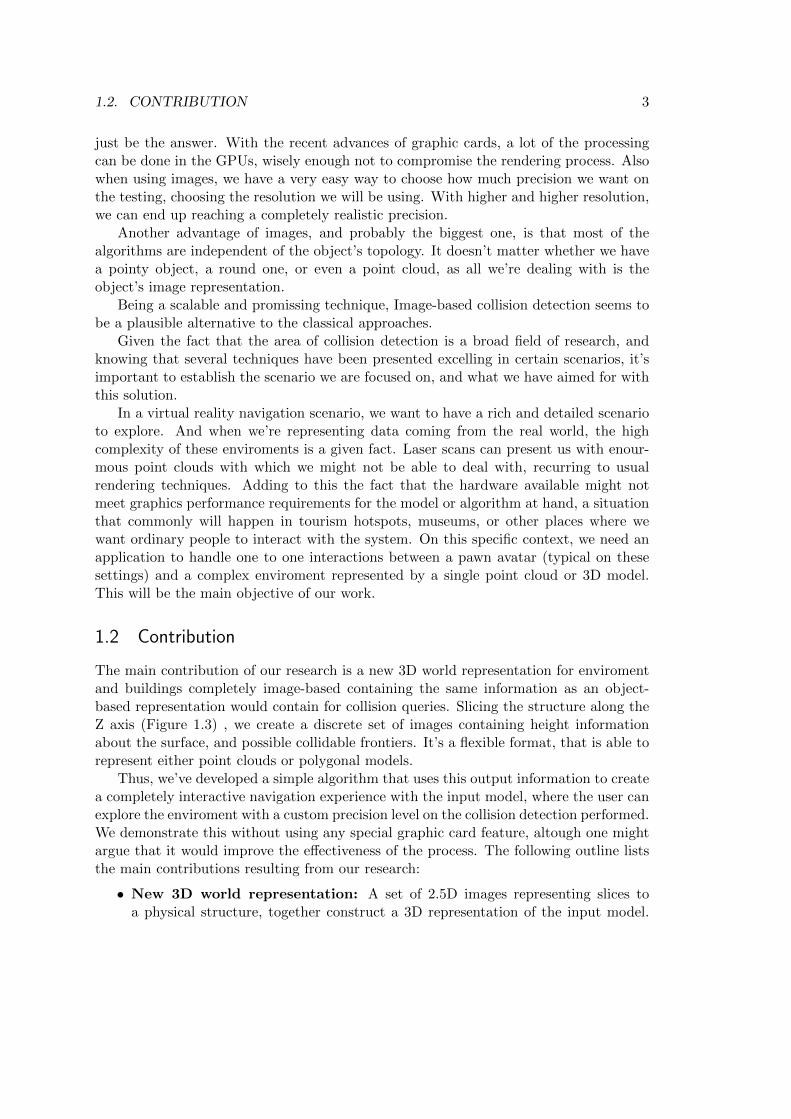
2.1 Representation from Loscos et. al [27] where an agent checks on the gridrepresentation for moving possibilities. On the second subimage from leftbeing capable of climbing a step, on the rightmost subimage being forcedto turn back. . . . . . . . . . . . . . . . . . . . . . . . . . . . . . . . . . . 8
2.2 Late 80’s low polygon count 3D model from Lin-canny paper . . . . . . . 9
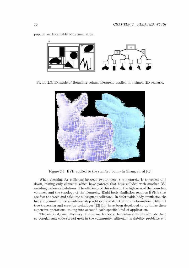
2.3 Example of Bounding volume hierarchy applied in a simple 2D scenario. . 10
2.4 BVH applied to the stanford bunny in Zhang et. al [42] . . . . . . . . . . 10
2.5 Illustration of stochastic collision detection, where pairs of randomly se-lected features are tracked as the objects approach each other . . . . . . . 12
2.6 LDI calculation . . . . . . . . . . . . . . . . . . . . . . . . . . . . . . . . . 13
2.7 Example of a medium-size point cloud rendered with QSplat (259.975points) . . . . . . . . . . . . . . . . . . . . . . . . . . . . . . . . . . . . . . 14
2.8 Point cloud with high point density . . . . . . . . . . . . . . . . . . . . . . 17
3.1 Height-map. Real terrain at left, output height-map at right . . . . . . . . 20
3.2 Pipeline of operations executed on the preprocessing stage in order tocreate the slices representation . . . . . . . . . . . . . . . . . . . . . . . . 21
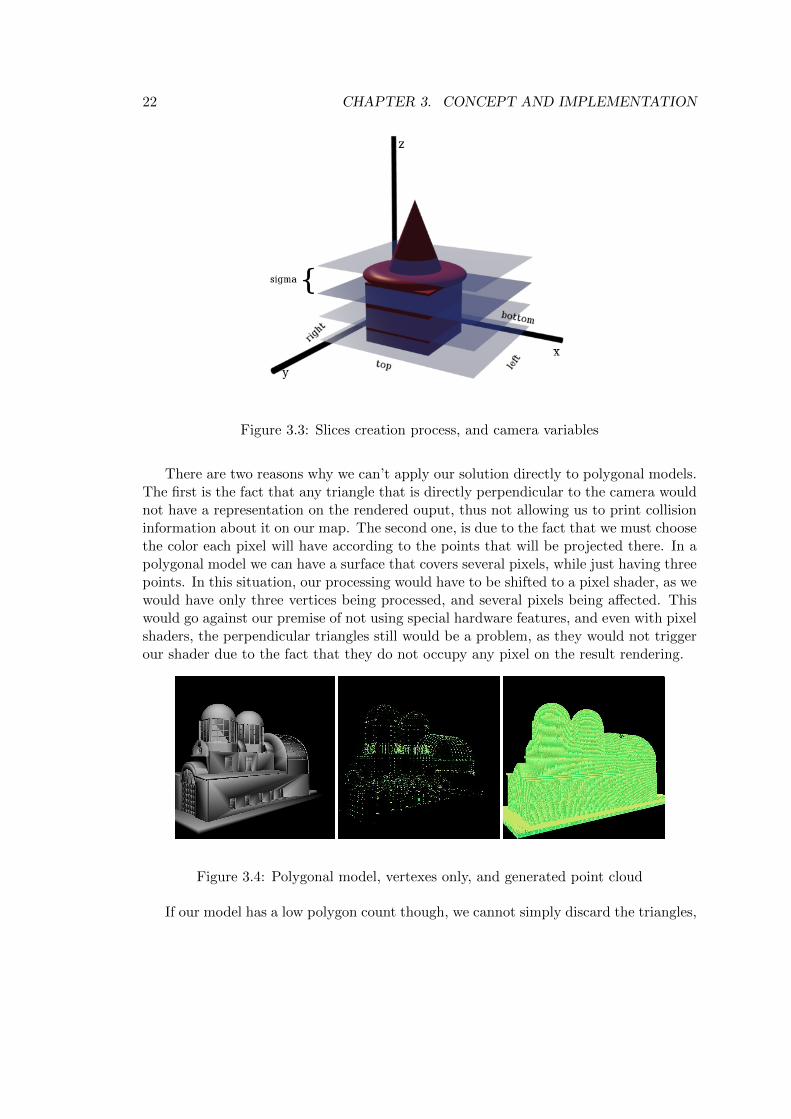
3.3 Slices creation process, and camera variables . . . . . . . . . . . . . . . . 22
3.4 Polygonal model, vertexes only, and generated point cloud . . . . . . . . . 22
3.5 oversampled Triangle . . . . . . . . . . . . . . . . . . . . . . . . . . . . . . 24
3.6 Result of subsample . . . . . . . . . . . . . . . . . . . . . . . . . . . . . . 25
3.7 Technique for surface orientation detection. Red points belong to a ver-tical structure, grey points to the floor. . . . . . . . . . . . . . . . . . . . . 27
3.8 Three slices of an office environment, where walls and floor are clearlydistinguished, aswell as a section of a roof on the entrance. . . . . . . . . 27
4.1 Models used as input for testing. . . . . . . . . . . . . . . . . . . . . . . . 32
ix

x LIST OF FIGURES
4.2 Graph picturing average time values in seconds for the pre-processingstage of each model and configuration. . . . . . . . . . . . . . . . . . . . . 34
4.3 Graph picturing memory cost in megabytes during the pre-processingstage of each model and configuration. . . . . . . . . . . . . . . . . . . . . 36
4.4 Memory used by the complete application at a given moment during run-time. . . . . . . . . . . . . . . . . . . . . . . . . . . . . . . . . . . . . . . . 36
4.5 Sequence of the first four maps of the input model Columns. . . . . . . . 384.6 Low resolution scenario: small round object interaction and floor collision. 39

List of Tables
2.1 Coarse granularity in the compromise between precision and efficiency. . . 15
4.1 Features of the models used for evaluation . . . . . . . . . . . . . . . . . . 334.2 Average frame-rate during evaluation . . . . . . . . . . . . . . . . . . . . . 354.3 Memory used for obstacle detection . . . . . . . . . . . . . . . . . . . . . . 364.4 Polygonal oversampling results . . . . . . . . . . . . . . . . . . . . . . . . 384.5 Comparison between point cloud techniques . . . . . . . . . . . . . . . . . 40
xi

xii LIST OF TABLES

List of Algorithms
3.1 Slices creation . . . . . . . . . . . . . . . . . . . . . . . . . . . . . . . . . . 213.2 Polygonal model oversampling . . . . . . . . . . . . . . . . . . . . . . . . . 233.3 Points coloring and obstacle detection . . . . . . . . . . . . . . . . . . . . 263.4 Broad-phase and collision detection . . . . . . . . . . . . . . . . . . . . . . 29
xiii

xiv LIST OF ALGORITHMS

Contents
1 Introduction 1
1.1 Problem and motivation . . . . . . . . . . . . . . . . . . . . . . . . . . . . 1
1.2 Contribution . . . . . . . . . . . . . . . . . . . . . . . . . . . . . . . . . . 3
1.3 Outline . . . . . . . . . . . . . . . . . . . . . . . . . . . . . . . . . . . . . 5
2 Related Work 7
2.1 Collision avoidance . . . . . . . . . . . . . . . . . . . . . . . . . . . . . . . 7
2.2 Collision detection . . . . . . . . . . . . . . . . . . . . . . . . . . . . . . . 8
2.2.1 Feature based . . . . . . . . . . . . . . . . . . . . . . . . . . . . . . 8
2.2.2 Bounding volumes hierarchies (BVH) . . . . . . . . . . . . . . . . 9
2.2.3 Stochastic techniques . . . . . . . . . . . . . . . . . . . . . . . . . 11
2.2.4 Image based . . . . . . . . . . . . . . . . . . . . . . . . . . . . . . . 11
2.3 Point Clouds . . . . . . . . . . . . . . . . . . . . . . . . . . . . . . . . . . 14
2.4 Comparison . . . . . . . . . . . . . . . . . . . . . . . . . . . . . . . . . . . 15
2.5 Summary . . . . . . . . . . . . . . . . . . . . . . . . . . . . . . . . . . . . 16
3 Concept and Implementation 19
3.1 Representation . . . . . . . . . . . . . . . . . . . . . . . . . . . . . . . . . 19
3.1.1 Slices creation . . . . . . . . . . . . . . . . . . . . . . . . . . . . . 20
3.1.2 Polygonal model oversampling . . . . . . . . . . . . . . . . . . . . 21
3.1.3 Information processing and encoding . . . . . . . . . . . . . . . . . 25
3.2 Collision detection . . . . . . . . . . . . . . . . . . . . . . . . . . . . . . . 28
3.2.1 Broad phase and collision detection . . . . . . . . . . . . . . . . . 28
3.2.2 Narrow phase and collision response . . . . . . . . . . . . . . . . . 29
3.3 Summary . . . . . . . . . . . . . . . . . . . . . . . . . . . . . . . . . . . . 30
4 Experimental Results 31
4.1 Environment and settings . . . . . . . . . . . . . . . . . . . . . . . . . . . 31
4.2 Pre-processing time and Memory usage . . . . . . . . . . . . . . . . . . . 33
4.3 Runtime . . . . . . . . . . . . . . . . . . . . . . . . . . . . . . . . . . . . . 34
4.4 Polygonal oversampling and Obstacle detection . . . . . . . . . . . . . . . 37
4.5 Collision detection and precision . . . . . . . . . . . . . . . . . . . . . . . 38
4.6 Evaluation . . . . . . . . . . . . . . . . . . . . . . . . . . . . . . . . . . . . 39
xv

xvi CONTENTS
5 Conclusion and Future work 415.1 Future work . . . . . . . . . . . . . . . . . . . . . . . . . . . . . . . . . . . 41
Bibliography 43

Chapter 1
Introduction
1.1 Problem and motivation
In rigid and deformable body simulation, virtual reality, games, and other types ofapplications where several 3D objects exist and interact, the proper execution of thecollision detection task results in a huge [htp] to realism. As objects move aroundand animate, their parts end up intersecting and if not detected and stopped, createunnatural behaviours that are unnaceptable in this domain of applications.
Collision detection is normally a bottleneck in the visualization and interaction pro-cess, as collisions need to be checked at each frame. Traditionally, the more complicatedand crowded is our scene, the more calculations need to be done, bringing our frame-ratedown. Therefore the optimization of this process, gaining speed without losing quality inthe simulation, is something that has been researched for years using different techniquesand approaches.
With a naive approach, the geometrical testing for intersections between all polygons,one will not have a scalable solution by any means, and will quickly overload the CPUwith work. So various techniques using bounding volumes, distance fields, and otherauxiliary data structures that group these polygons together or exclude useless testings,have been developed so less testing is needed at each frame.
Invariantly, in more complex (Figure 1.1) or crowded (Figure 1.2) scenes, where wewish to keep some degree of realism, hence using more or tighter bounding volumes,once again one quickly reaches a performance bottleneck. Also, in scenarios that use adifferent object representation such as a point cloud, we can’t rely on object topologyinformation. The classical approaches either won’t work, or will have to heavily adaptto this specific scenario, tayloring its optimizations to a point cloud representation.
Even with simpler scenes, sometimes one might not have enough processing poweravailable. Somehow we need to avoid the problem of overloading the CPU with collisiondetection tests, and reduce the number of times we need to lookup data structures, sothat the simulation is runnable even on a less capable machine, for example a kiosksetting.
Using images as an alternative way of executing the task of collision detection might
1

2 CHAPTER 1. INTRODUCTION
Figure 1.1: Highly detailed 3D model with 100 million polygons
Figure 1.2: Scene with 15.000 watermelons from Oblivion, a game by Obsidian, andpoint cloud data from real world laser scan.
1.2. CONTRIBUTION 3
just be the answer. With the recent advances of graphic cards, a lot of the processingcan be done in the GPUs, wisely enough not to compromise the rendering process. Alsowhen using images, we have a very easy way to choose how much precision we want onthe testing, choosing the resolution we will be using. With higher and higher resolution,we can end up reaching a completely realistic precision.
Another advantage of images, and probably the biggest one, is that most of thealgorithms are independent of the object’s topology. It doesn’t matter whether we havea pointy object, a round one, or even a point cloud, as all we’re dealing with is theobject’s image representation.
Being a scalable and promissing technique, Image-based collision detection seems tobe a plausible alternative to the classical approaches.
Given the fact that the area of collision detection is a broad field of research, andknowing that several techniques have been presented excelling in certain scenarios, it’simportant to establish the scenario we are focused on, and what we have aimed for withthis solution.
In a virtual reality navigation scenario, we want to have a rich and detailed scenarioto explore. And when we’re representing data coming from the real world, the highcomplexity of these enviroments is a given fact. Laser scans can present us with enour-mous point clouds with which we might not be able to deal with, recurring to usualrendering techniques. Adding to this the fact that the hardware available might notmeet graphics performance requirements for the model or algorithm at hand, a situationthat commonly will happen in tourism hotspots, museums, or other places where wewant ordinary people to interact with the system. On this specific context, we need anapplication to handle one to one interactions between a pawn avatar (typical on thesesettings) and a complex enviroment represented by a single point cloud or 3D model.This will be the main objective of our work.
1.2 Contribution
The main contribution of our research is a new 3D world representation for enviromentand buildings completely image-based containing the same information as an object-based representation would contain for collision queries. Slicing the structure along theZ axis (Figure 1.3) , we create a discrete set of images containing height informationabout the surface, and possible collidable frontiers. It’s a flexible format, that is able torepresent either point clouds or polygonal models.
Thus, we’ve developed a simple algorithm that uses this output information to createa completely interactive navigation experience with the input model, where the user canexplore the enviroment with a custom precision level on the collision detection performed.We demonstrate this without using any special graphic card feature, altough one mightargue that it would improve the effectiveness of the process. The following outline liststhe main contributions resulting from our research:
• New 3D world representation: A set of 2.5D images representing slices toa physical structure, together construct a 3D representation of the input model.

4 CHAPTER 1. INTRODUCTION
Figure 1.3: Illustration of how our representation represents a 3D object
Each 2D map contains precise information about surfaces and collidable frontiers,this precision is defined by the density of the points in the model, and the desiredresolution of the output images.
• Multi-tier solution for collision detection: In a first phase, a possible collisioncan be identified in constant time, leaving more precise testing to a second tier.This division allows us to freely adapt the application to the requirements needed.
• Simple but precise collision response: A simple algorithm using our new3D world representation has been developed to allow basic navigation on a inputenviroment. Only using the simple broad phase collision detection algorithm and2D collision response, we have achieved a precise interaction that works on a 3Denvironment.
• An input independent algorithm: Point clouds and polygonal models (trian-gle meshes, CAD, etc) are processed in a similar way, making our representationeffective in both cases. These are the main inputs we will be receiving on thedescribed scenario.
• High scalability and efficiency: A collision detection technique that is onlyaffected by input complexity on a pre-processing stage, and has close to no impacton the rendering cycle of the application, thus not representing a bottleneck onthe visualization cycle.

1.3. OUTLINE 5
1.3 Outline
This document describes throughly the research carried out and the developed work inthe following structure:
• Chapter 1: Introduction, problem and motivation, resulting contributions.
• Chapter 2: Description of the related work on collision detection and avoidance,highlighting the most influential research on each field and comparing and analyz-ing their performance on our chosen scenario.
• Chapter 3: Concept and implementation details. We describe each step of thepre-processing stage where the slices representation is created, followed by both thebroad-phase collision detection process and the narrow-phase and collision responseoperation.
• Chapter 4: Test results and performance evaluation of our work on several as-pects. A critical analysis and comparison with other work on the community isalso made.
• Chapter 5: Conclusion and overview of possible improvements on the developedwork.

6 CHAPTER 1. INTRODUCTION

Chapter 2
Related Work
Given that the problem of computing object’s collisions is not only present in the areasof virtual reality, games and simulations, but also in different fields such as artificialintelligence and robotics, there is quite a vast amount of work often optimized for thedifferent respective contexts that can mislead our research in the wrong direction. Evenwhen talking about collision detection in a single domain, such as simulations, twoapplications may still be hugely different regarding requirements and concerns. Theattributes of the objects such as defformability, breakability or surface material bring upnew algorithms and techniques to solve these problems in an efficient way. Therefore, westart by establishing the difference between collision avoidance and collision detection,then a short overview of relevant work on processing point clouds is given, followedby a classification and an overview of the most relevant work in the virtual realitycommunity, and finally, a short conclusion fitting our research in the given state of theart. For further information on collision detection and avoidance techniques we suggestthe following surveys: [34] [9] [40]
2.1 Collision avoidance
The goal of collision avoidance is to predict an upcoming collision, and use this infor-mation to prevent it from happening. It is normaly used in crowd simulations, or anyother environment where the object to avoid colliding is an intelligent agent. This workdiffers from collision detection in the way that we just need to identify the objects in theworld, and avoid intersecting with them, not letting it happen and then correcting it asone would do when walking in the real world. This can be achieved through intelligentworld perception and representation.
The collision can be avoided in many different ways. In the BOIDS framework [36]simple circular spheres are used to detect obstacles in the vicinity. On Ondrej et. al [35]work, a more complex technique is presented that simulates the human vision to detectobstacles on the agent’s path. ClearPath [10] uses the concept of Velocity Obstacles,that takes into account the velocity of the other objects in the scene, and how thecurrent object’s velocity should adapt to avoid a collision. Finally, Loscos et. al [27]
7
8 CHAPTER 2. RELATED WORK
Figure 2.1: Representation from Loscos et. al [27] where an agent checks on the gridrepresentation for moving possibilities. On the second subimage from left being capableof climbing a step, on the rightmost subimage being forced to turn back.
represent the environment as patches to where the agent can or cannot go according toit’s occupation.
After the several different presented techniques are applied, different methods tocalculate the detour of the agent to avoid that obstacle are used. Some of the techniquesinvolve complex mathematical systems, other techniques are basic, such as stopping theagent for a while. This already belongs to a domain in Robotics called path planning,unrelated to what’s covered in our work.
2.2 Collision detection
Different lines of work have been developed in the area of collision detection. Each ofthe techniques has developed a unique representation of the world and it’s objects, beingapplied differently and with certain advantages in each specific domain of applications.Simple games and environment navigation can work well with simple bounding volumesor distance fields, while cloth simulation and deformable body require tighter volumes,hierarchies, or combining efforts with Image or feature based techniques. It’s importantto keep in mind that all these techniques have a field where they excel, therefore it’simportant to consider all of their capabilities when working in collision detection
2.2.1 Feature based
These algorithms use the vertices, edges and faces (so called features) of the object’sboundary to perform geometric computations to determine if a pair of polyhedra intersectand possibly calculate the distance between them. The 1988 work from Moore andWilhelms [31] describes the mathematical process of detecting the intersection betweentwo polygons. Other famous examples are the Lin-Canny algorithm[24] and it’s morerecent related algorithm, V-Clip[29]. In V-Clip they keep track of the closest featuresbetween two objects, in this way they derive both the separation distance, and thevertices that have possibly already penetrated the other object, something that wasn’tpossible with the Lin-Canny Algorithm. This technique called Voronoi Marching [29]has been applied in SWIFT [7], where a hierarchical representation of convex polyhedra

2.2. COLLISION DETECTION 9
that englobes the features is created, and the algorithm is applied to each level of thehierarchy. These algorithms have been used mostly in robotics and path planning, sincethese algorithms don’t behave very well when objects penetrate each other. On the otherhand, the mathematics behind simple polygon intersection is still sometimes used whena detailed collision detection is needed. Given the high number of triangles of today’s3D models, this technique is never used alone. It may be easily associated with BVHsin the lower levels.
Figure 2.2: Late 80’s low polygon count 3D model from Lin-canny paper
2.2.2 Bounding volumes hierarchies (BVH)
Being by far the most popular class of collision detection algorithms, being applied suc-cessfully in every research area, BVHs work by dividing the objects in smalller primitivescontained by it, until a certain leaf criteria is achieved (top-down approach) or starting onthe smallest primitives possible, grouping up until a single volume is achieved (bottom-up) as illustrated in Figure 2.3. Each primitive is enveloped by a particular boundingvolume shape, for example the Sphere [17] which is the most popular approach, the Ori-ented Bounding Box (OBB) [14] and the Discrete Oriented Polytope (DOP), a convexobject made of k planes that envelop the primitive. The Axis Aligned Bounding Box(AABB) [22] [13] [42] is the most used version of the latter, being a k-DOP [?, kdop]ithk=6. Each of these volumes has a particular advantage: Spheres are easier to fit, OBBshave faster pruning capabilities, and AABBs are quicker to update, therefore being very
10 CHAPTER 2. RELATED WORK
popular in deformable body simulation.
Figure 2.3: Example of Bounding volume hierarchy applied in a simple 2D scenario.
Figure 2.4: BVH applied to the stanford bunny in Zhang et. al [42]
When checking for collisions between two objects, the hierarchy is traversed top-down, testing only elements which have parents that have collided with another BV,avoiding useless calculations. The efficiency of this relies on the tightness of the boundingvolumes, and the topology of the hierarchy. Rigid body similation requires BVH’s thatare fast to search and calculate subsequent collisions. In deformable body simulation thehierarchy must in one simulation step refit or reconstruct after a deformation. Differenttree traversing and creation techniques [22] [14] have been developed to optimize theseexpensive operations, taking into accound each specific kind of application.
The simplicity and efficiency of these methods are the features that have made themso popular and wide-spread used in the community. although, scalability problems still
2.2. COLLISION DETECTION 11
exist with BVH’s. We don’t always have a balanced and prunable tree, and when higherfidelity on more complex models is needed, the number of bounding volumes may endup increasing very fast, making all the previous operations very costly. Even with amodel with simple genus, if we seek more fidelity in the collision detection, we need toheavily increase the number of bounding volumes to approach a realistic solution as seenin Figure 2.4.
2.2.3 Stochastic techniques
Stochastic algorithms that try to give a faster but less exact answer have been devel-oped, giving the developer the option to ”buy” exactness in collisions with computingpower. Uno and Slater [41] present a study regarding the sensibility of people to exactcollision response, stating that humans cannot distinguish between physically-correctand physically-plausible behaviour. Relaxing the collision criteria may lead to fasterand lighter algorithms.
The ”Average-case” approach is applied in BVHs, not really checking for intersectionsbetween volumes in the hierarchy, but calculating the probability that they containintersecting polygons. In BVH’s based on spatial subdivision, this would mean tryingto find a grid that contained several polygons from object A and object B, intersectingwith high probability. The technique based on Randomly selected Primitives [?, ?, MT]selects random pairs of features that are probable to collide, and calculates the distancebetween them. The local minima is kept for the next step and calculations are onceagain made. The exact collision pairs are derived with Lin-Canny [24] feature basedalgorithm.
With a similar idea, Kimmerle et. al [37] have applied BVH’s with lazy hierarchyupdates and stochastic techniques to defformable objects and cloth. After detectingcollision between the bounding volumes, pairs of features contained in this volumes arerandomly selected, and temporal coeherence between them is kept, updating the pairs tothe closest neighbour (Figure 2.5). When a threshold of proximity is reached, a collisionis declared, and thus, corrected.
Although a plausible result is achieved, it is impossible to reach a physically-correct orexact simulation with these techniques. In certain domains such as VR medical surgerysuch uncertainty is unacceptable, and when dealing with point clouds, penetrations arespecially unnatural to see. Also, as these techniques rely largely on Bounding volumeshierarchies, they still share some of the same disadvantages mentioned earlier, speciallywhen dealing with unstructured data such as point clouds or polygon soups.
2.2.4 Image based
Several image-space techniques have been developed recently, as the advance of graphiccards has made their implementation not only viable in terms of processing power andmemory allocation, but it has become simpler to implement these techniques using theprogrammable graphic units.

12 CHAPTER 2. RELATED WORK
Figure 2.5: Illustration of stochastic collision detection, where pairs of randomly selectedfeatures are tracked as the objects approach each other
The algorithms commonly work with the projection of the objects, opposed to theprevious techniques that work in object space. RECODE [5] transforms the probem ofthree-dimensional collision detection to a one-dimensional interval test along the Z-axis.By using a mask in the stencil buffer based on one of the two objects coordinates (Zmaxor Zmin) a stencil test is made, and the result tells us if the two objects overlap or not.This stencil test is also the base of several other works that try to take advantage ofthe new graphic cards capabilities [21] [32], and are also being extended to achieve selfcollision in deformable objects [4].
Hoff et. al [8] treat 2D collisions using the bounding boxes to detect possible colli-sions, and then creating a grid of that region, enabling proximity queries to be made usingthe graphics hardware to detect overlapping polygons, hence allowing several queries tobe done regarding the intersection.
2.2. COLLISION DETECTION 13
CULLIDE [15] uses occlusion queries only to detect potentially colliding objects,and then triangle intersection is made on the CPU. Collisions are detected based on asimple lemma that states: ”An object O does not collide with a set of objects S if Ois fully visible with respect to S.” they can quickly prune objects from the pottentiallycolliding set (PCS). Rendering bounding volumes of the objects in normal and reverselist storage order, they remove the objects that are fully visible in both passes. Thisis applied iteratively until there is no change in the PCS. Boldt and Meyer [6] haveextended this algorithm to contemplate self collisions, exchanging the ”lesser than” testin the depth buffer for a ”lesser than or equal”, thus guaranteeing that self collisionswould be detected, however unfortunately they create some performance problems withclosed objects, that clearly will never be fully visible in relation to themselves, thus neverleaving the PCS.
The recognized capability of culling and quickly avoiding useless collision tests whenworking in image-space has been recognized and applied in [19], where closest pointquery is implemented in the Z-buffer, aided by a convex hull that is created envelopinga target number of polygons.
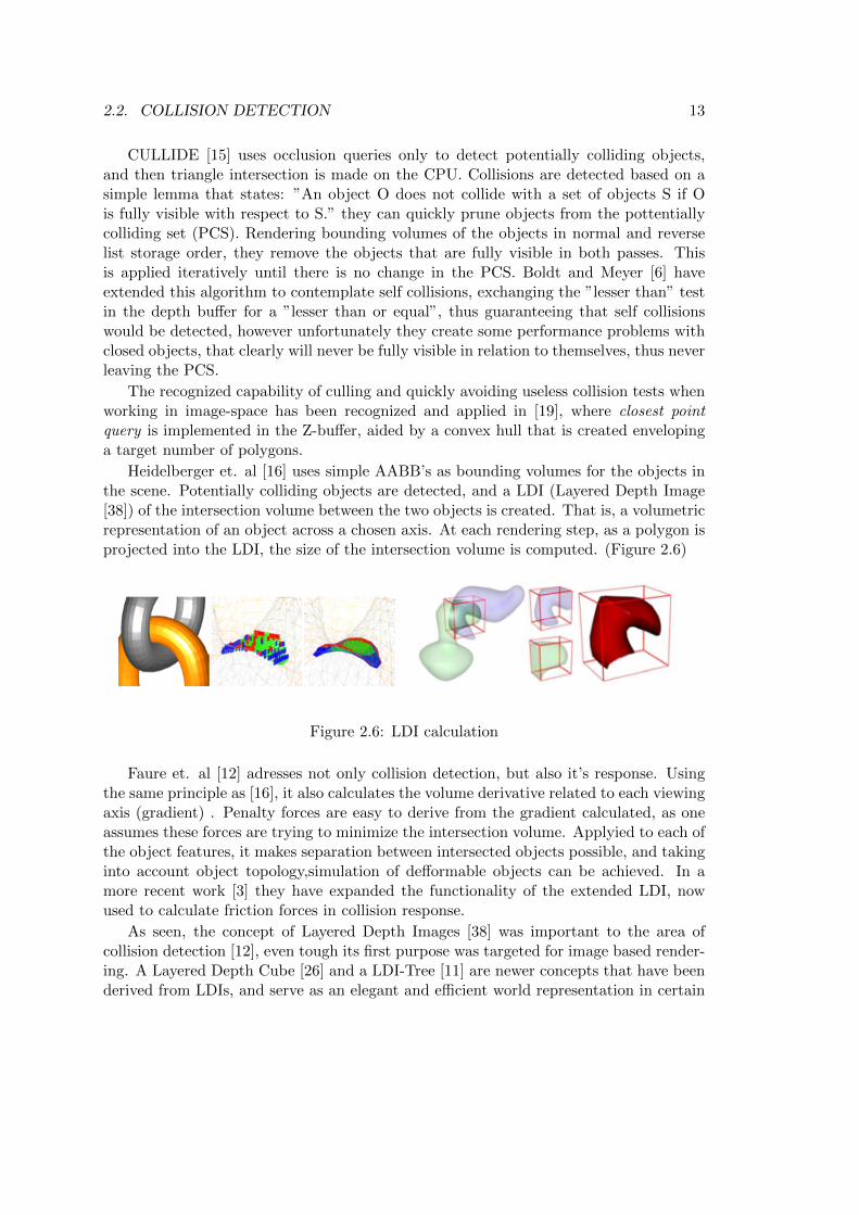
Heidelberger et. al [16] uses simple AABB’s as bounding volumes for the objects inthe scene. Potentially colliding objects are detected, and a LDI (Layered Depth Image[38]) of the intersection volume between the two objects is created. That is, a volumetricrepresentation of an object across a chosen axis. At each rendering step, as a polygon isprojected into the LDI, the size of the intersection volume is computed. (Figure 2.6)
Figure 2.6: LDI calculation
Faure et. al [12] adresses not only collision detection, but also it’s response. Usingthe same principle as [16], it also calculates the volume derivative related to each viewingaxis (gradient) . Penalty forces are easy to derive from the gradient calculated, as oneassumes these forces are trying to minimize the intersection volume. Applyied to each ofthe object features, it makes separation between intersected objects possible, and takinginto account object topology,simulation of defformable objects can be achieved. In amore recent work [3] they have expanded the functionality of the extended LDI, nowused to calculate friction forces in collision response.
As seen, the concept of Layered Depth Images [38] was important to the area ofcollision detection [12], even tough its first purpose was targeted for image based render-ing. A Layered Depth Cube [26] and a LDI-Tree [11] are newer concepts that have beenderived from LDIs, and serve as an elegant and efficient world representation in certain

14 CHAPTER 2. RELATED WORK
domains. In a scene where the polygon count, or point count, is too high to be stored,an image is a much more compact representation.
2.3 Point Clouds
Point clouds are the result of a 3D laser scan, normally used to create 3D CAD models formanufatured parts, building inspection or visualization, and sometimes animation. Theinformation is not commonly used exactly as it was captured, normally being prepro-cessed first. Noise removal, surface reconstruction, are some of the operations performed.
Nowadays, 3D laser scans have made possible for one to create a model with hundredsof millions of polygons. As ordinary simplification and display algorithms are impraticalfor such massive data sets, rendering techniques for point-clouds have been developedso we can discard polygon information, and still have a realistic visualization.
QSplat [39] uses a multiresolution hierarchy based on bounding spheres to render highcomplexity meshes that are transformed into point clouds, and has been applied on themuseum kiosk scenario described on Chapter one. Lars Linsen [25] has also worked withpoint cloud visualization without needing triangle information, in contrast with QSplat[39] which uses this information if available, otherwise estimating the normals by fittinga plane to the vertices in a small neighbourhood around each point. These techniqueshave made point cloud representation more viable on a real interactive application, asthey are already clearly lighter than the traditional ones.
Figure 2.7: Example of a medium-size point cloud rendered with QSplat (259.975 points)
Several surface reconstruction techniques have been developed. Some techniquesuse the idea from Marching Cubes algorithm [23] [33] and convert the point cloud into

2.4. COMPARISON 15
a volumetric distance field, thus reconstructing the implicit surface. Poisson SurfaceReconstruction [18] can reconstruct the surfaces with high precision and has been appliedin 3D mesh processing applications such as MeshLab [28] . These reconstructions aremade so that the models can be used as polygonal meshes. It still differs from a handmade CAD model where objects are divided and coherently structured making collisiondetection easier.
Regarding collision detection, algorithms using feature based techniques, boundingvolumes, and spatial subdivision have been developed. Similar to the idea presented inSWIFT [7], Klein and Zachmann [20] create bounding volumes on groups of points socollision detection can be normally applied. Figueiredo et. al [13] uses spatial subdivisionto group points in the same voxel, and BVHs to perform collision detection.
With point cloud data resulting from 3D laser scans, the tight fitting of the boundingboxes becomes less and less reliable due to the non constant density of points, as statedby Figueiredo et. al [13]. Performing Image-based collision detection, the precision ofthe detection is directly proportional to the characteristics/quality of the input, sincewe work with the visual representation of the point cloud, not needing to estimate thefrontiers of the object.
Although they present us with apparent advantages on this scenario, Image Basedtechniques still haven’t been applied or studied in this domain.
2.4 Comparison
Having adressed these techniques and stated their advantages and disadvantages, wecan see what a tight competition it is. There is no perfect technique that casts a hugeshadow over the others. Each of them has a different and innovative approach to theproblem, and has an edge over the others in certain situations. In Table 1 we have aquick comparison of the refered techniques.
Table 2.1: Coarse granularity in the compromise between precision and efficiency.
Advantages Disadvantages
Feature based Simple implementation, pre-cise
Not Scalable
BVH Popular implementation, rela-tively scalable, reliable
Compromise between preci-sion and efficiency hard to ob-tain, requires input data to beproperly segmented
Stochastic Fast and adaptable Not completely reliable,shares all of BVH’S issues.
Image-based Scalable and precise, topologyindependent, works with un-structured polygon soups
Requires specific graphic cardcapabilities
Feature based algorithms are the pioneers of this area, and used to work with low-

16 CHAPTER 2. RELATED WORK
polygon 3D models, there are situations where they perform very well, but suffer withpolygon counts commonly found today. That is why some more recent approaches suchas SWIFT [7] started to rely on hierarchical representations such as the ones used inBVH’s. These, besides being the most used technique nowadays, are far from beingperfect. Scalability is achieved with better hierarchies and bounding volumes loosening.Such a compromise between efficiency and quality/realism is hard, yet achievable, evenwith high complexity models. While dealing with point clouds, there are techniques[20] [13] that create bounding volumes in groups of points, simillary to what was donein feature based algorithms. Besides being a viable answer, we still face the questionbetween efficiency and precision.
Stochastic techniques give us the capability of choosing the precision of our testsvery easily, and have also been used with point clouds, since the basis of some of theseworks is point-wise comparsion. But we can’t expect a completely correct simulationwhen running these algorithms, the compromise between efficiency and quality/realismbeing harder to achieve on these situations.
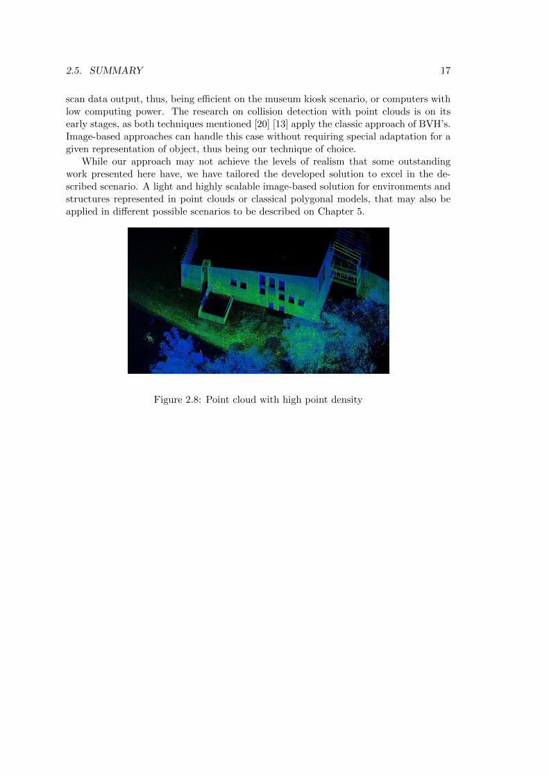
With Image based techniques, we can perform collision detection with complex ob-jects [12] since we are working on image-space, and the number of objects can be quicklypruned as shown in CULLIDE [15], thus guaranteeing scalability. The precision of thetesting can also be chosen by choosing the resolution of the images, and if we needed, wecan theoretically have as much precision as feature based algorithms. By treating theobjects in image space, we are not dependant on the type of object we are working with.Point clouds can be efficiently dealt with, since the increase in the number of points takesus closer to a closed surface as shown in Figure 2.8 (even more evident when viewed ata distance) thus working to our advantage.
One drawback that could be stated, is the graphic cards capabilities that they mayrequire. The work described in the next chapter, has not required any special featureto be implemented. Everything, all the calculations were done on the CPU, althoughsome steps could be speeded up if implemented on the graphic card, Practical resultsand the concept itself of image-based collision detection show that it is viable withoutthose capabilities.
2.5 Summary
Even though research on collision detection has been sucessfuly advancing throughoutthe last years, a technique that works perfectly well in every scenario has not yet beendeveloped, pushing us towards developing different approaches to excel in each specificscenario. Being the most traditional approach, BVH’s have been experimented in severaldifferent scenarios, being effective in most of these scenarios, but outshined by image-based techniques or stochastic approaches in specific situations, such as cloth simulationand deformable objects. Image-based collision detection has not yet been applied tocertain scenarios, mainly due to the fact that it is a recent field.
As shown in section 2.3, point cloud representation is a viable and light alternativeregarding data structures and visualization, and most probably the optimal one for laser
2.5. SUMMARY 17
scan data output, thus, being efficient on the museum kiosk scenario, or computers withlow computing power. The research on collision detection with point clouds is on itsearly stages, as both techniques mentioned [20] [13] apply the classic approach of BVH’s.Image-based approaches can handle this case without requiring special adaptation for agiven representation of object, thus being our technique of choice.
While our approach may not achieve the levels of realism that some outstandingwork presented here have, we have tailored the developed solution to excel in the de-scribed scenario. A light and highly scalable image-based solution for environments andstructures represented in point clouds or classical polygonal models, that may also beapplied in different possible scenarios to be described on Chapter 5.
Figure 2.8: Point cloud with high point density

18 CHAPTER 2. RELATED WORK

Chapter 3
Concept and Implementation
This chapter presents the developed work in full detail. We present an innovative Image-based object representation in section 3.1 and describe the pre-processing step where itis created. Section 3.2 describes how we can apply this representation in the collisiondetection task in a broad and in a narrow phase.
3.1 Representation
Image-based algorithms that have been presented in the community ([15] [5] [21] [6] [3][12]) perform very well in various kinds of scenarios, but some features of our set scenario(described on chapter 1.1) make them hard or impossible to be applied (e.g. our data isunstructured, not all objects are closed or convex).
Besides working with traditional models, we also receive point clouds as inputs. Thesenormaly cover a large set of objecs, and do not provide us with any object structure.This makes it hard or even impossible to fit traditional bounding boxes around eachindividual object as done on the work from Faure et. al [3] [12] . Also, when dealingwith navigation, one may go completely inside buildings and structures. This situationassociated with the lack of segmentation of the scene, makes it impossible for some ofthe approaches to work ([5] [16] [15] [5] [21] [6]) ), since they rely on polygons of closedobjects that define their boundaries, telling them whether there is a collision or not.
In not so complicated scenarios, images have been used for collision avoidance. Thework from Loscos et. al [27] as an example, uses a 2.5D map of the city showing whichpositions were occupied by walls or other solid objects by painted pixels. Also, there isa height information associated to the objects to distinguish whether the agent couldor couldn’t climb that obstacle, such as a small step. This simple representation of a2D tone map, can be used for collision detection. Similar techniques have been appliedalready on the 2D era of gaming, where collisions were calculated pixel-wise.
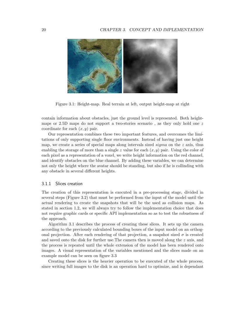
This idea of a 2.5D map has been extented to a height-map on a terrain visualizationcontext as shown on figure 3.1, where a color code is used to represent the height of acertain point on the map. This representation holds more information than the mapson ClearPath [27], but cannot be used for collision avoidance or detection, as it does not
19
20 CHAPTER 3. CONCEPT AND IMPLEMENTATION
Figure 3.1: Height-map. Real terrain at left, output height-map at right
contain information about obstacles, just the ground level is represented. Both height-maps or 2.5D maps do not support a two-stories scenario , as they only hold one zcoordinate for each (x, y) pair.
Our representation combines these two important features, and overcomes the limi-tations of only supporting single floor environments. Instead of having just one heightmap, we create a series of special maps along intervals sized sigma on the z axis, thusenabling the storage of more than a single z value for each (x, y) pair. Using the color ofeach pixel as a representation of a voxel, we write height information on the red channel,and identify obstacles on the blue channel. By adding these variables, we can determinenot only the height where the avatar should be standing, but also if he is collinding withany obstacle in several different heights.
3.1.1 Slices creation
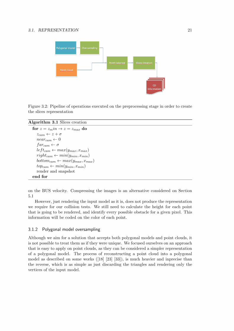
The creation of this representation is executed in a pre-processing stage, divided inseveral steps (Figure 3.2) that must be performed from the input of the model until theactual rendering to create the snapshots that will be the used as collision maps. Asstated in section 1.2, we will always try to follow the implementation choice that doesnot require graphic cards or specific API implementation so as to test the robustness ofthe approach.
Algorithm 3.1 describes the process of creating these slices. It sets up the cameraaccording to the previously calculated bounding boxes of the input model on an orthog-onal projection. After each rendering of that projection, a snapshot sized σ is createdand saved onto the disk for further use.The camera then is moved along the z axis, andthe process is repeated until the whole extension of the model has been rendered ontoimages. A visual representation of the variables mentioned and the slices made on anexample model can be seen on figure 3.3
Creating these slices is the heavier operation to be executed of the whole process,since writing full images to the disk is an operation hard to optimize, and is dependant
3.1. REPRESENTATION 21
Figure 3.2: Pipeline of operations executed on the preprocessing stage in order to createthe slices representation
Algorithm 3.1 Slices creation
for z = zmin→ z = zmax dozcam ← z + σnearcam ← 0farcam ← σleftcam ← max(ymax, xmax)rightcam ← min(ymin, xmin)bottomcam ← max(ymax, xmax)topcam ← min(ymin, xmin)render and snapshot
end for
on the BUS velocity. Compressing the images is an alternative considered on Section5.1
However, just rendering the input model as it is, does not produce the representationwe require for our collision tests. We still need to calculate the height for each pointthat is going to be rendered, and identify every possible obstacle for a given pixel. Thisinformation will be coded on the color of each point.
3.1.2 Polygonal model oversampling
Although we aim for a solution that accepts both polygonal models and point clouds, itis not possible to treat them as if they were unique. We focused ourselves on an approachthat is easy to apply on point clouds, as they can be considered a simpler representationof a polygonal model. The process of reconstructing a point cloud into a polygonalmodel as described on some works ([18] [23] [33]), is much heavier and inprecise thanthe reverse, which is as simple as just discarding the triangles and rendering only thevertices of the input model.
22 CHAPTER 3. CONCEPT AND IMPLEMENTATION
Figure 3.3: Slices creation process, and camera variables
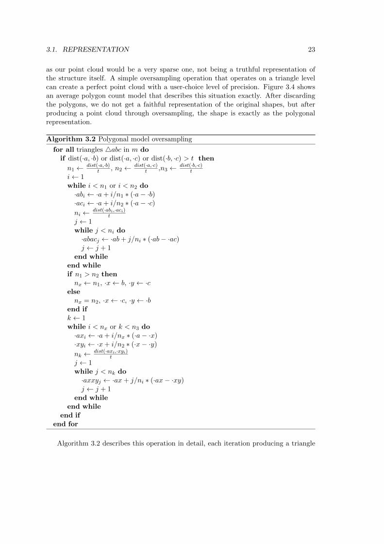
There are two reasons why we can’t apply our solution directly to polygonal models.The first is the fact that any triangle that is directly perpendicular to the camera wouldnot have a representation on the rendered ouput, thus not allowing us to print collisioninformation about it on our map. The second one, is due to the fact that we must choosethe color each pixel will have according to the points that will be projected there. In apolygonal model we can have a surface that covers several pixels, while just having threepoints. In this situation, our processing would have to be shifted to a pixel shader, as wewould have only three vertices being processed, and several pixels being affected. Thiswould go against our premise of not using special hardware features, and even with pixelshaders, the perpendicular triangles still would be a problem, as they would not triggerour shader due to the fact that they do not occupy any pixel on the result rendering.
Figure 3.4: Polygonal model, vertexes only, and generated point cloud
If our model has a low polygon count though, we cannot simply discard the triangles,
3.1. REPRESENTATION 23
as our point cloud would be a very sparse one, not being a truthful representation ofthe structure itself. A simple oversampling operation that operates on a triangle levelcan create a perfect point cloud with a user-choice level of precision. Figure 3.4 showsan average polygon count model that describes this situation exactly. After discardingthe polygons, we do not get a faithful representation of the original shapes, but afterproducing a point cloud through oversampling, the shape is exactly as the polygonalrepresentation.
Algorithm 3.2 Polygonal model oversampling
for all triangles 4abc in m doif dist(·a, ·b) or dist(·a, ·c) or dist(·b, ·c) > t then
n1 ← dist(·a,·b)t , n2 ← dist(·a,·c)
t ,n3 ← dist(·b,·c)t
i← 1while i < n1 or i < n2 do·abi ← ·a+ i/n1 ∗ (·a− ·b)·aci ← ·a+ i/n2 ∗ (·a− ·c)ni ← dist(·abi,·aci)
tj ← 1while j < ni do·abacj ← ·ab+ j/ni ∗ (·ab− ·ac)j ← j + 1
end whileend whileif n1 > n2 thennx ← n1, ·x← b, ·y ← ·c
elsenx = n2, ·x← ·c, ·y ← ·b
end ifk ← 1while i < nx or k < n3 do·axi ← ·a+ i/nx ∗ (·a− ·x)·xyi ← ·x+ i/n2 ∗ (·x− ·y)
nk ← dist(·axi,·xyi)t
j ← 1while j < nk do·axxyj ← ·ax+ j/ni ∗ (·ax− ·xy)j ← j + 1
end whileend while
end ifend for
Algorithm 3.2 describes this operation in detail, each iteration producing a triangle
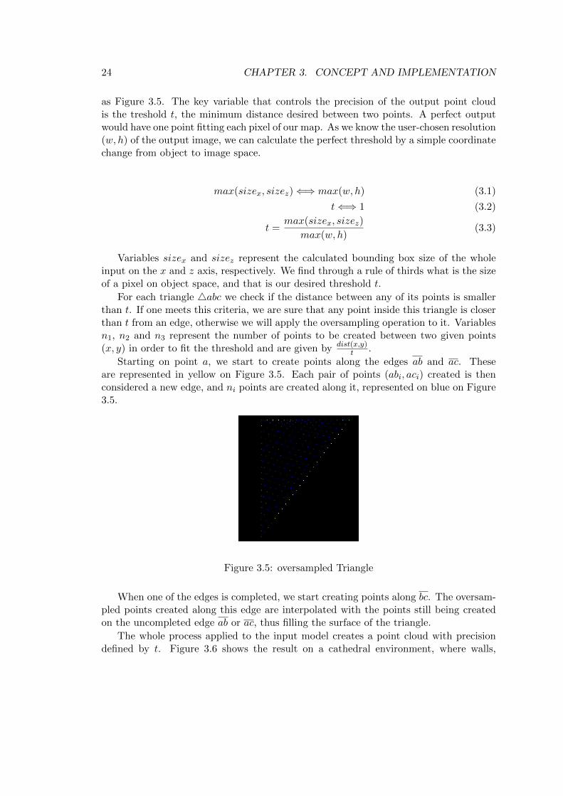
24 CHAPTER 3. CONCEPT AND IMPLEMENTATION
as Figure 3.5. The key variable that controls the precision of the output point cloudis the treshold t, the minimum distance desired between two points. A perfect outputwould have one point fitting each pixel of our map. As we know the user-chosen resolution(w, h) of the output image, we can calculate the perfect threshold by a simple coordinatechange from object to image space.
max(sizex, sizez)⇐⇒ max(w, h) (3.1)
t⇐⇒ 1 (3.2)
t =max(sizex, sizez)
max(w, h)(3.3)
Variables sizex and sizez represent the calculated bounding box size of the wholeinput on the x and z axis, respectively. We find through a rule of thirds what is the sizeof a pixel on object space, and that is our desired threshold t.
For each triangle 4abc we check if the distance between any of its points is smallerthan t. If one meets this criteria, we are sure that any point inside this triangle is closerthan t from an edge, otherwise we will apply the oversampling operation to it. Variablesn1, n2 and n3 represent the number of points to be created between two given points(x, y) in order to fit the threshold and are given by dist(x,y)
t .
Starting on point a, we start to create points along the edges ab and ac. Theseare represented in yellow on Figure 3.5. Each pair of points (abi, aci) created is thenconsidered a new edge, and ni points are created along it, represented on blue on Figure3.5.
Figure 3.5: oversampled Triangle
When one of the edges is completed, we start creating points along bc. The oversam-pled points created along this edge are interpolated with the points still being createdon the uncompleted edge ab or ac, thus filling the surface of the triangle.
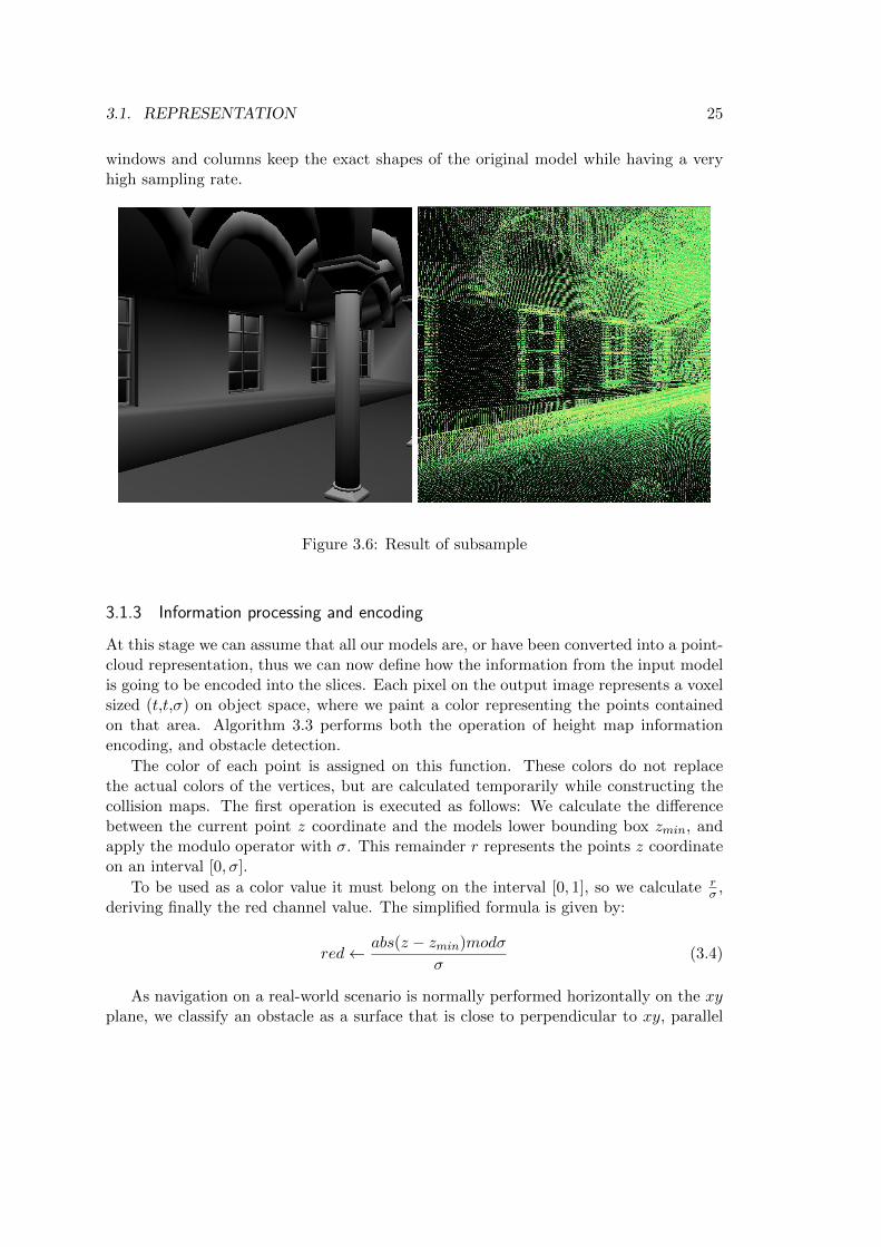
The whole process applied to the input model creates a point cloud with precisiondefined by t. Figure 3.6 shows the result on a cathedral environment, where walls,
3.1. REPRESENTATION 25
windows and columns keep the exact shapes of the original model while having a veryhigh sampling rate.
Figure 3.6: Result of subsample
3.1.3 Information processing and encoding
At this stage we can assume that all our models are, or have been converted into a point-cloud representation, thus we can now define how the information from the input modelis going to be encoded into the slices. Each pixel on the output image represents a voxelsized (t,t,σ) on object space, where we paint a color representing the points containedon that area. Algorithm 3.3 performs both the operation of height map informationencoding, and obstacle detection.
The color of each point is assigned on this function. These colors do not replacethe actual colors of the vertices, but are calculated temporarily while constructing thecollision maps. The first operation is executed as follows: We calculate the differencebetween the current point z coordinate and the models lower bounding box zmin, andapply the modulo operator with σ. This remainder r represents the points z coordinateon an interval [0, σ].
To be used as a color value it must belong on the interval [0, 1], so we calculate rσ ,
deriving finally the red channel value. The simplified formula is given by:
red← abs(z − zmin)modσ
σ(3.4)
As navigation on a real-world scenario is normally performed horizontally on the xyplane, we classify an obstacle as a surface that is close to perpendicular to xy, parallel

26 CHAPTER 3. CONCEPT AND IMPLEMENTATION
Algorithm 3.3 Points coloring and obstacle detection
for all points p in m dos← floor(abs(z−zmin)
σ )
red← abs(z−zmin)modσσ
redold ← cube[xscreen][yscreen][s]if abs(redold − red) ∗ σ > σε thencube[xscreen][yscreen][s]← 1p.color(red, 1, 1)if redold > red thenp.z ← p.z + (redold − red) ∗ σ + ε2
end ifelsecube[xscreen][yscreen][s]← redp.color(red, 1, 0.1)
end ifend for
to zy or zx. This is a simple assumption clearly present in the real world, simplifyingour obstacle detection algorithm in detecting possible vertical surfaces on a point cloud.
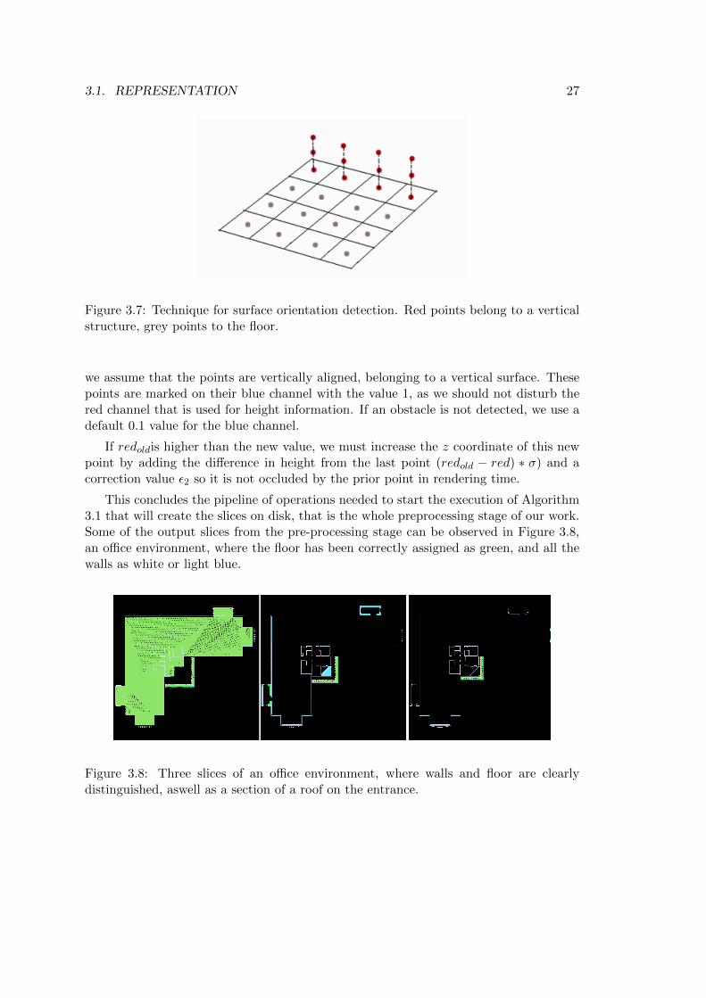
Although techniques for surface normals estimation have been developed [30], wechoose a simpler approach since we do not require a precise value for the normal, butjust an estimation of how paralel to the z axis it is. Figure 3.7 describes briefly thisestimative operation executed on algorithm 3.3. Points lined up vertically on the samepixel are most likely to belong to a vertical surface.
To guarantee that on a given slice we will have at least two points that belong to anobstacle lined up to be projected on that slice, we define the slice size σ as 3t. Since onoversampled point clouds we have a distance of t between every point, a slice sized 3twill certainly have at least two points lined up to be projected on it. On natural pointclouds, we define t as the minimum distance between two points. On these scenarios, thedistance between points is normally constant, except on places where we have scanningflaws. So the minimum distance covers the well scanned surfaces of the point cloud.
Each position on the 3D array cube[w][h][σ] represents a voxel on object space, ora pixel on the output image. This data structure is necessary to store for each voxelwhich points will be projected onto a certain pixel, thus enabling us to perform obstacledetection. The values written on this 3D array will not be used for map creation, sincethey only store a single float value representing the maximum height of a point projectedon this position. Collision information is coded on each point red and blue channel.
At each step, after calculating the red value of the given point, we store this valueon a position of the array. If there is already a stored value on this voxel, the differencebetween both red values is calculated, and transformed into an object-space distanceabs(redold − red) ∗ σ
If this difference is bigger than a certain small percentage ε of the size σ of the slice,
3.1. REPRESENTATION 27
Figure 3.7: Technique for surface orientation detection. Red points belong to a verticalstructure, grey points to the floor.
we assume that the points are vertically aligned, belonging to a vertical surface. Thesepoints are marked on their blue channel with the value 1, as we should not disturb thered channel that is used for height information. If an obstacle is not detected, we use adefault 0.1 value for the blue channel.
If redoldis higher than the new value, we must increase the z coordinate of this newpoint by adding the difference in height from the last point (redold − red) ∗ σ) and acorrection value ε2 so it is not occluded by the prior point in rendering time.
This concludes the pipeline of operations needed to start the execution of Algorithm3.1 that will create the slices on disk, that is the whole preprocessing stage of our work.Some of the output slices from the pre-processing stage can be observed in Figure 3.8,an office environment, where the floor has been correctly assigned as green, and all thewalls as white or light blue.
Figure 3.8: Three slices of an office environment, where walls and floor are clearlydistinguished, aswell as a section of a roof on the entrance.

28 CHAPTER 3. CONCEPT AND IMPLEMENTATION
3.2 Collision detection
During the last decade, the field of collision detection has evolved beyond the task ofpreventing objects form overlapping. Deformable objects have been mentioned in severalworks ([16] [4] [22] [42]) aswell as self-intersections([4] [6]) and even the effect of friction[12] has already been implemented on a virtual scenario. But considering the contextgiven on Section 1.1 where we consider point clouds as a viable input, the challenge ofavoiding two objects to overlap is renewed.
The developed representation provides us with enough information to perform quickcollision detection on this environment. While the aspects concerning the realism ofthe collision response have not been explored, precision on simple rigid bodies collisiondetection has been achieved.
We divide the task of collision detection into two steps: a first step, that we callBroad phase, where we verify the occurance of collisions between any objects in thescene, and a second step called narrow phase, where we perform collision response.
3.2.1 Broad phase and collision detection
This task consists on identifying possible collisions between all objects on the scene. Byrepresenting the avatar that will be navigating on the environment by an Axis AlignedBounding Box (AABB), we first calculate its size in pixels by calculating pixx ← sizex
t
and pixz ← sizeyt , where threshold t was calculated as the pixel size. This will be the
number of pixels checked for collision on each slice, around the center of the pawn. Therange of slices that will be actually needed to calculate collision detection with the pawnare given by:
slice0 ←zpawnmin + zpawn− zmin
σ(3.5)
slicen ←zpawnmax + zpawn− zmin
σ(3.6)
These are the only images we will need to load into the memory at the same time inorder to perform collision detection. Since the transition between different heights whileexploring a model is normally linear, that implies that we do not have sudden jumps orchanges in height. Each time a new map is needed and it is not on RAM, we will loadthem from the Hard disk.
We only load new slices onto memory until a user defined constant nslices is reached.New slices beyond this point, replace an already loaded slice that has the furthest z valuefrom the avatar’s own z value, meaning it is not needed at this point of the execution.While we want to minimize memory usage, we also want to load the slices from the diskas few times as possible.
To detect possible collisions, we check from slice0 to slicen, the pixels repesentingthe bounding box of the avatar on its current position on image-space (xview, yview). Ifany checked pixel is not black, we mark the object as colliding, and will be processed ina narrow phase. The process is explained in detail on Algorithm 3.4.
3.2. COLLISION DETECTION 29
Algorithm 3.4 Broad-phase and collision detection
pixx ← sizext , pixz ← sizey
tslice0 ← zpawnmin+zpawn−zmin
σ , slicen ← zpawnmax+zpawn−zminσ
for all slice s in (slice0, ..., slicen) doif s not loaded thenload(s)
end iffor i← xview − pixx
2 to i← xview + pixx2 do
for j ← yview − pixy2 to j ← yview +
pixy2 do
if slice[s][i][j].color not black thenreturn TRUE
end ifend for
end forend forif nloaded > nslices thenunload()
end ifreturn FALSE
This implementation does not require any graphic card features, as all tests are doneCPU-wise. The worst case complexity of Algorithm 3.4 is O(pixx ∗ pixy ∗ s), dependingon the resolution of the image, the size of the avatar, and the density of the point cloud.Alternative and arguably faster techniques that can be implemented on hardware arediscussed on Section 5.1
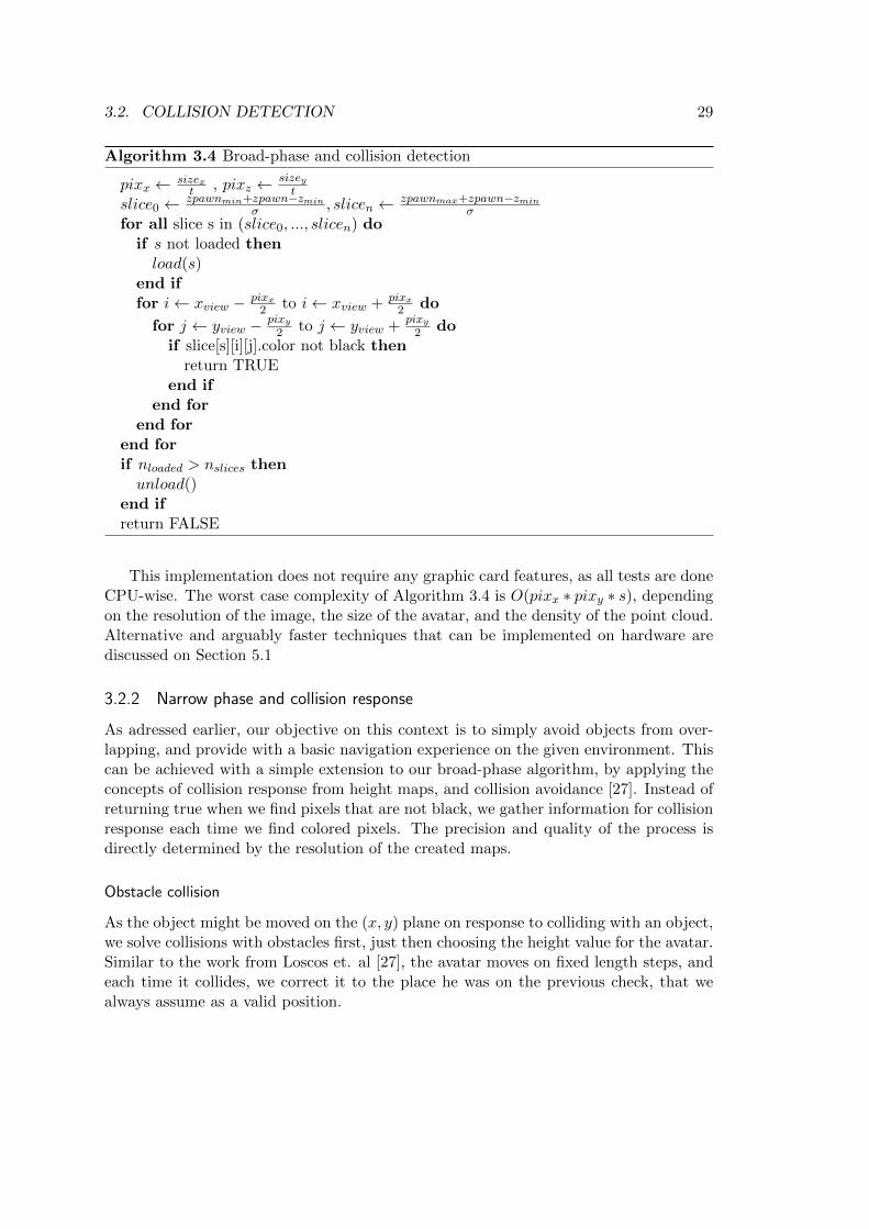
3.2.2 Narrow phase and collision response
As adressed earlier, our objective on this context is to simply avoid objects from over-lapping, and provide with a basic navigation experience on the given environment. Thiscan be achieved with a simple extension to our broad-phase algorithm, by applying theconcepts of collision response from height maps, and collision avoidance [27]. Instead ofreturning true when we find pixels that are not black, we gather information for collisionresponse each time we find colored pixels. The precision and quality of the process isdirectly determined by the resolution of the created maps.
Obstacle collision
As the object might be moved on the (x, y) plane on response to colliding with an object,we solve collisions with obstacles first, just then choosing the height value for the avatar.Similar to the work from Loscos et. al [27], the avatar moves on fixed length steps, andeach time it collides, we correct it to the place he was on the previous check, that wealways assume as a valid position.

30 CHAPTER 3. CONCEPT AND IMPLEMENTATION
The size of this fixed length step is divided by two so the pawn can move a little closerto the obstacle, and reset after no collision is detected. Pixels with the blue channel setto 1 always represent an obstacle, except on applications where we want to enable theavatar to climb small obstacles, as the agents from Loscos et.al [27]. On these situations,we may ignore these pixels up until the height we want to be considered as climbable.
We apply this (x, y) correction each time an obstacle pixel is found on the processdescribed in Algorithm 3.4, until all the pixels representing the avatar’s bounding boxare verified.
Floor interaction
Height is defined exactly as it is on height maps. Multiplying the coded height informa-tion on the red channel by σ and adding the z base coordinate of the given slice, we haveprecise information about the given point’s height. Collision response can be made bysetting the final height to the average height of the points on the base of the boundingbox, or by the maximum value. Here also we check for surface height values from thefirst slice until the height we want to consider as climbable.
The complexity of this operation is exactly O(pixx ∗ pixy ∗ s), but without addingany extra operation from the broad phase checking. Faster implementations and consid-erations about multi-avatar scenarios will be discussed on section 5.1
3.3 Summary
This chapter has covered completely the process of image-based collision detection onpoint clouds and polygonal models oversampled into point clouds using our new multi-layered approach. By assiging colors to each point at the pre-processing stage, identifyingobstacles by estimating how close their normals are to the z axis, we write informationabout the whole input structure on several 2D projections of 3D volumes sized σ. Thenumber of images created, the precision of the collision detection progress, and thedensity of the point cloud are all values determined by the user when the resolution ofthe images is chosen. This provides us with a powerful adaptation capability, regardingdifferent scenarios and machines.

Chapter 4
Experimental Results
4.1 Environment and settings
We have implemented the whole algorithm using OpenGL 2.1.2, C and the OpenGLUtility Toolkit (GLUT) to deal with user input and the base application loop managing.OpenGL is a standard across different computing architectures and operating systems,and our solution is aimed to be efficient without depending on the environment, makingit a natural choice.
The platform used for testings is a computer with a Intel core 2 Duo CPU at 2 GHzwith 2GB of RAM, a NVIDIA GeForce 9400 adapter, running Microsoft Windows Sevenx86. Seven models have been used for testing, each representing different scenarios andstyles of modeling. None of them was tailored in a specific way to our application, asmost of them were downloaded from free 3D models repositoriums on the web [2] [1]. Amore detailed overview of them can be seen on Table 4.1
Although some models such as Office (Figure 4.1a) have a low complexity, the polyg-onal oversampling process creates even more dense point clouds than our real worldinputs, Room (Figure 4.1f) and Entrance (Figure 4.1g). Results of this oversampling arediscussed on Section 4.4 together with obstacle detection, and presented on Table 4.4.
Section 4.2 will discuss the pre-processing stage speed and memory usage on differentmodels, resolutions, and point coloring options. These will give us an overview of thescalability of the representation, and how these different settings affect our performance.Section 4.5 will evaluate the results of collision detection regarding precision on differentscenarios, using a simple rectangular pawn representing a bounding box of a given avataras an user controlled pawn that navigates the environment on an established path.
Section 4.6 will add all the results together and make a critical evaluation of the de-veloped work, regarding its applicability on the described scenario and other consideredpossibilities, and how does it perform when compared to other techniques described inChapter 2 regarding the tested aspects.
31

32 CHAPTER 4. EXPERIMENTAL RESULTS
(a) Office (b) Church
(c) Sibenik (d) Columns
(e) Streets (f) Room
(g) Entrance
Figure 4.1: Models used as input for testing.

4.2. PRE-PROCESSING TIME AND MEMORY USAGE 33
Table 4.1: Features of the models used for evaluation
Model Type Complexity Details
Office Polygonal 17.353 pts Office environment with cubiclesand hallways
Church Polygonal 26.721 pts Simple church with stairs andcolumns
Sibenik Polygonal 47.658 pts Cathedral of St. James on Sibenik,Croatia
Columns Polygonal 143.591 pts Big environment with localizedcomplexity.
Room 3D laser Scan 271.731 pts 3D Scan of a room with chairs, atable, and other objects.
Street Polygonal 281.169 pts Outside street environment with anirregular floor, houses, and severalobjects.
Entrance 3D laser Scan 580.062 pts Entrance of the Batalha monasteryin Portugal.
4.2 Pre-processing time and Memory usage
Creating the 3D representation during the pre-processing stage is the task on the pipelinethat is most cpu intensive, since after the representations are created, the applicationtends to remain stable with regular frame rate and memory usage, only to be eventuallydisturbed by the process of loading new slices. Four rounds of tests have been donefor each model using two different image resolutions (700x700 and 350x350), performingobstacle detection (signaled by a + on Figures 4.2 and 4.3) and one without it (signaledby a - on Figures 4.2 and 4.3). This provides us with enough information about the keyvariables that make the difference on the efficiency of this stage. Resolution, obstacledetection, and polygonal oversampling.
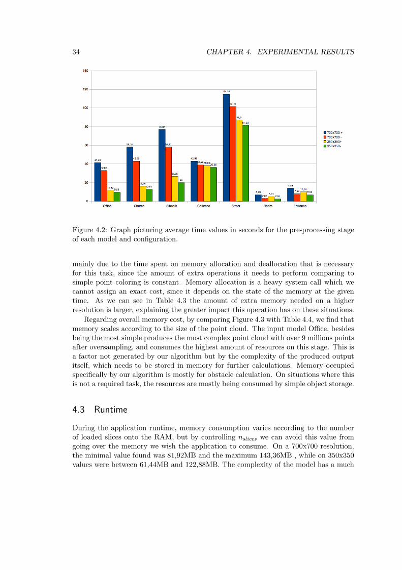
Figure 4.2 shows the time taken on the whole preprocessing stage for each modeland configuration. The clock is started as OpenGL is setting up, and stops when everyimage has been written to disk. By analysing the graph, we conclude that the most cpudemanding task on the pipeline is polygonal oversampling, since the two other testedinputs, the point clouds, were the faster inputs to process, besides having a higher pointcomplexity than the original polygonal models. More detail on this task will be givenon Section 4.4.
The increase on processing time with point clouds is linear to point complexity, sincethe time has doubled between Room and Entrance, while they have close to a 2:1 ratioon their point count. This linear growth is expected since each point must be checkedfor coloring once, and also for common input processing such as input file reading anddisplay list creation.
There is also an expected extra cost in time for obstacle calculation, and this is
34 CHAPTER 4. EXPERIMENTAL RESULTS
Figure 4.2: Graph picturing average time values in seconds for the pre-processing stageof each model and configuration.
mainly due to the time spent on memory allocation and deallocation that is necessaryfor this task, since the amount of extra operations it needs to perform comparing tosimple point coloring is constant. Memory allocation is a heavy system call which wecannot assign an exact cost, since it depends on the state of the memory at the giventime. As we can see in Table 4.3 the amount of extra memory needed on a higherresolution is larger, explaining the greater impact this operation has on these situations.
Regarding overall memory cost, by comparing Figure 4.3 with Table 4.4, we find thatmemory scales according to the size of the point cloud. The input model Office, besidesbeing the most simple produces the most complex point cloud with over 9 millions pointsafter oversampling, and consumes the highest amount of resources on this stage. This isa factor not generated by our algorithm but by the complexity of the produced outputitself, which needs to be stored in memory for further calculations. Memory occupiedspecifically by our algorithm is mostly for obstacle calculation. On situations where thisis not a required task, the resources are mostly being consumed by simple object storage.
4.3 Runtime
During the application runtime, memory consumption varies according to the numberof loaded slices onto the RAM, but by controlling nslices we can avoid this value fromgoing over the memory we wish the application to consume. On a 700x700 resolution,the minimal value found was 81,92MB and the maximum 143,36MB , while on 350x350values were between 61,44MB and 122,88MB. The complexity of the model has a much

4.3. RUNTIME 35
lighter impact here, being only noticable on tasks that are unrelated to collision detectionsuch as rendering and shading.
Table 4.2 shows the average frame-rate during the execution of our application foreach model. Two tests were made for each model, one where we performed collisiondetection, and the other where we did not. Results show that our algorithm did notaffect the rendering speed of the interactive application at all, environments where theframe rate was below the values considered minimum for interaction would be on thissituation with any other collision detection algorithm applied to it. And this low frame-rate on these situations was only due to other process on the visualization cycle such asshading, present on polygonal models such as Street but not on the point clouds. Thisshows that our technique is clearly not the bottleneck of the visualization cycle, one ofthe main concerns presented on Section 1.1.
Table 4.2: Average frame-rate during evaluation
Model Collision Simple
Office 60 fps 60 fps
Church 60 fps 60 fps
Sibenik 60 fps 60 fps
Colums 30 fps 30 fps
Street 19 fps 19 fps
Room 60 fps 60 fps
Entrance 30 fps 30 fps
The amount of memory needed to perform collision detection on a very dense pointcloud is close to the same needed on a simple one. Figure 4.4 shows the consumption ofmemory with the minimum loaded number of slices needed, and confirms the excelentscalability of our technique in this scenario.
As stated before, the preprocessing stage can be executed only once for a givenconfiguration, as every generated image is written to disk and can be loaded on furtherinteractions. After the first interaction for any input model, our technique does not needany setup time to work, so the linear growth on time and memory seen on Figures 4.2and 4.3 will only be applied once, leaving further interactions with the scalable behaviourshown on Figure 4.4.

36 CHAPTER 4. EXPERIMENTAL RESULTS
Figure 4.3: Graph picturing memory cost in megabytes during the pre-processing stageof each model and configuration.
Figure 4.4: Memory used by the complete application at a given moment during runtime.
Table 4.3: Memory used for obstacle detection
Model 700x700 350x350
Office 65,54 MB 20,48 MB
Church 151,55 MB 16,38 MB
Sibenik 249,86 MB 38,86 MB
Colums 45,06 MB 8,19 MB
Street 122,88 MB 16,38 MB
Room 51,2 MB 20,48 MB
Entrance 69,63 MB 16,38 MB
4.4. POLYGONAL OVERSAMPLING AND OBSTACLE DETECTION 37
4.4 Polygonal oversampling and Obstacle detection
Part of the complexity of polygonal oversampling as described on Algorithm 3.2 lieson the resolution needed for the output images, since our approach is to try to obtaina perfect point cloud that will fill all the pixels on the destined image sized (w, h).Resolution affects greatly the complexity of the produced point clouds as shown onTable 4.4, where we can see that in some cases such as Church and Office the size ofthe output has tripled, while we only doubled the resolution. For street, this ratio isdifferent, as the size of the output only doubled.
The number of produced points will not scale linearly with the size of the output,because the algorithm does not create a fixed number of new points on each step. If wewould create x new points for each input triangle, we would have a highly irregular pointcloud, since triangles of a 3D model do not share the same size. Our process creates asmany points as necessary to fit the calculated threshold, and this is harder to achieve insome models than others.
The input model Columns (Figure 4.1d) besides having the second highest trianglecomplexity at start, it produces the simplest point cloud after oversampling. Most ofits triangles are concentrated on a certain area on the middle of the model, and therest being covered by a flat and simple surface, wasting precious resolution. Analysingthe produced maps on Figure 4.5 we see that the first map from the left fully utilizesthe determined 750x750 resolution, while the second from the left uses 250x250, andthat value goes down to 170x170 on the other two. The reduced effective resolutiondiminishes the need to subsample the triangles, producing a less dense point cloud.
Obstacle detection showed good results on all scenarios, identifying correctly everysurface aligned with the z axis with isolated errors on single pixels that do not affectthe collision detection process. However, due to the nature of the algorithm, we areunable to precisely state what is the limit angle on a surface from where it starts to beidentified as an obstacle. The closer it is to being aligned with the z, more pixels start tobe marked as obstacles. This results have proved to be precise enough for the simulationon Church and to be performed without errors while the pawn was going through theramp.
although loss of precision happens on certain situations where we have localizedcomplexity, on rich and homogeneous environments, the oversampling operation providesus with detailed point clouds that produce maps able to represent every obstacle andsurface with fidelity. On Figure 3.8 we can see perfectly detailed walls, and Figure4.5 shows columns and steps with high precision aswell, fulfilling the purpose of theoversampling that was creating visually closed surfaces just like the original polygons,so the image representation kept as much detail as possible.

38 CHAPTER 4. EXPERIMENTAL RESULTS
Figure 4.5: Sequence of the first four maps of the input model Columns.
Table 4.4: Polygonal oversampling results
Model Original 350x350 700x700
Office 17.353 pts 3.088.193 pts 9.349.585 pts
Church 26.721 pts 2.246.549 pts 6.475.125 pts
Sibenik 47.658 pts 1.838.167 5.199.093 pts
Columns 143.591 pts 1.448.383 pts 2.612.303 pts
Street 281.169 pts 3.606.225 pts 7.142.361 pts
4.5 Collision detection and precision
Results on collision detection have been verified through establishing a fixed route tonavigate with the pawn where it goes through different situations and scenarios. The firstpath is on Office where straight hallways and doors are tested, the second tests climbingstairs and going through a ramp on Cathedral, and the third interaction verifies irregularfloors and small and round obstacles, on a section of Street.
These scenarios have been tested with the ordinary two different resolutions setup,and for the steps and ramps experiment we have used two different values of nslices,so we could study the effect of reading a map on runtime. A high nslices keeps moreimages on RAM at the same time , while a low value has to read maps from disks morefrequently, but consumes less memory.
Tests on Cathedral have showed us that reading from the disk on runtime has abigger impact on efficiency than storing a higher number of images. When reading ahigh resolution image from disk, we notice a sudden drop on the frame-rate, and thisis well noticed when the pawn falls from a higher structure. Increasing nslices to storeenough slices to represent the ground floor and the platform on top of the steps, littleto no difference was noticed on memory load, and the interaction was a lot smoother.On a low resolution though, reading from disk on runtime showed no impact on theperformance.
The technique described on 3.2.2 for narrow phase and collision response does not tryto achieve maximum precision, since our objective is to have a simple interactive appli-cation with a real-world model. However, our technique has presented precise results onall scenarios and resolutions. Floor collision has shown to be highly reliable due to the
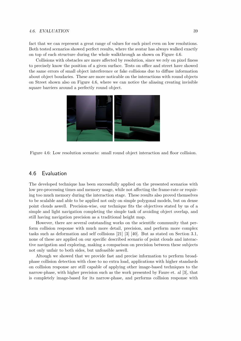
4.6. EVALUATION 39
fact that we can represent a great range of values for each pixel even on low resolutions.Both tested scenarios showed perfect results, where the avatar has always walked exactlyon top of each structure during the whole walkthrough as shown on Figure 4.6.
Collisions with obstacles are more affected by resolution, since we rely on pixel finessto precisely know the position of a given surface. Tests on office and street have showedthe same errors of small object interference or fake collisions due to diffuse informationabout object boudaries. These are more noticable on the interactions with round objectson Street shown also on Figure 4.6, where we can notice the aliasing creating invisiblesquare barriers around a perfectly round object.
Figure 4.6: Low resolution scenario: small round object interaction and floor collision.
4.6 Evaluation
The developed technique has been successfully applied on the presented scenarios withlow pre-processing times and memory usage, while not affecting the frame-rate or requir-ing too much memory during the interaction stage. These results also proved themselvesto be scalable and able to be applied not only on simple polygonal models, but on densepoint clouds aswell. Precision-wise, our technique fits the objectives stated by us of asimple and light navigation completing the simple task of avoiding object overlap, andstill having navigation precision as a traditional height map.
However, there are several outstanding works on the scientific community that per-form collision response with much more detail, precision, and perform more complextasks such as deformation and self collisions [21] [3] [40]. But as stated on Section 3.1,none of these are applied on our specific described scenario of point clouds and interac-tive navigation and exploring, making a comparison on precision between these subjectsnot only unfair to both sides, but unfeasible aswell.
Altough we showed that we provide fast and precise information to perform broad-phase collision detection with close to no extra load, applications with higher standardson collision response are still capable of applying other image-based techniques to thenarrow-phase, with higher precision such as the work presented by Faure et. al [3], thatis completely image-based for its narrow-phase, and performs collision response with

40 CHAPTER 4. EXPERIMENTAL RESULTS
excellence.The work on point cloud collision detection using boundig voulme hierarchies from
Figueiredo et. al [13] has been tested on one of our experimental scenarios, the Entranceof the Batalha Monastery, on a machine with a slightly faster processing speed andRAM than the one used for our walkthoughs. Table 4.5 shows a comparison betweenboth results, where we picked Oct 4096 for results, since it was shown in the paper tobe the one with the best performance.
Table 4.5: Comparison between point cloud techniques
Image-based BVH’s
Frame-rate 30 fps 16 to 30 fps
Total Memory 143.36 MB 225,44 MB
Pre-processing time 13.9 s 1500 s
Frame-rate was disturbed during the collision detection process on the R-tree aproach,while it remained steady at the 30 fps during the whole execution of our application.Also, the image-based technique has required much less memory to be executed, evenwith a high number of slices loaded onto memory. The biggest difference is in the pre-processing times. Our approach was executed 107 times faster than the BVH approach,and most importantly, this pre-processing stage must only be performed once for eachconfiguration, since the representation is written to the hard disk and can be used onfurther interactions.
As stated on Section 2.3 the research on point cloud collision detection is recent,and inexistent regarding image-based techniques. Our pioneer solution has presentedexcellent results, not only performing better than other works on point clouds publishedin the scientific community, but also being flexible enough to be applied on models fromCAD, or combined with precise collision response techniques. Without adding any loadto the visualization pipeline, our technique is not only scalable with input complexity, butalso with hardware capabilities. Image-based collision detection can be performed withour representation on any computer that can render the input model at an acceptableframe-rate, without requiring anything meaningful from the CPU or GPUs.
Chapter 5
Conclusion and Future work
A new image-based environment representation for collision detection has been pre-sented, using 2.5+D slices of an environment or building across the z axis. These imagescontain at each pixel, information about a certain voxel, representing it’s contents withcolors. Height map information is stored on the red channel, and obstacles are indicatedon the blue channel. This allows us to have a Broad phase collision detection stage thatis performed with high efficiency and scalability, where the user can choose the precisionaccording to the computing power at hand by simply adjusting the resolution of the pro-duced images. Point clouds and polygonal models are ubiquitously processed, makingour approach the top alternative for fast interaction with massive laser scan data.
Combining well with several existent aproaches for narrow-phase collision response,but also presenting a new and precise technique for this task, this work fills a gap in thearea of collision detection, exploring a scenario that has been receiving more attentionrecently. By solving one of the many issues we face while working with virtual realityand simulation, we have presented one more argument in favor of point clouds as a viablealternative to classical polygon representation in certain specific application scenarios.
5.1 Future work
Our work has fulfilled all of its objectives, however, there are several aspects that stillcan be improved or fine tuned not only to make it faster or more precise, but also toexplore several different application where this new approach can be applied.
As stated on Section 1.1, the advance of nowadays graphic cards are transformingyesterday’s special features into the basic kit of an average personal computer. SinceGPUs are designed to process images, we can use them to move some of the calculationsaway from the CPU to improve the algorithm’s performance. Our broad phase techniqueperforms several checks to single pixels of the images loaded onto memory. This taskcould be executed faster by doing a stencil test to determine if there are any pixels onthe area covered by the pawn. If any pixel would pass, a collision could be imediatlydetected.
Also, the point coloring algorithm still requires a large amount of memory to simulate
41

42 CHAPTER 5. CONCLUSION AND FUTURE WORK
rendering buffers in memory, where we project the points onto virtual pixels, and checkif they are occupied to perform obstacle detection, then assigning them an accordingcolor. By implementing this as a vertex shader, we would do exactly the same operation,without allocating extra memory, but using the buffers themselves. As each vertex wasprocessed, we would be checking and writing colors from the frame buffer, performingthe same operation without needing any extra memory allocation.
Although this representation was tested specifically on a scenario where we have onerich environment and only one avatar, it may be applied to several different situations.A multi-user scenario is possible, performing inter-object collision. This can be achievedby cross-checking both image representations for occupied pixels. Also, not limiting thesliced representation only to structures, but also applying it to the pawns and any otherobject on the scene. Applying this layered representation to rich and detailed objectssuch as the famous statue of David or the Stanford bunny and creating an interactiveapplication with it can be viable given the great scalability of our technique.
Another improvement that can be done is to try to solve the loss of effective resolutionthat was detected on the test model called ”Columns”. A solution that uses non-uniformresolution images, that meaning they use more pixels to store information about complexsections of the model, and group pixels containing the same information on regions wherethere are no objects. Similar ideas to some image compression techniques like Run lenghtencoding could be applied to achieve this objective.
Image comparison techniques can also be used to discard slices that do not add muchinformation to the last loaded slice, not only saving memory space, but possibly reducingdrastically the number of times our application needs to perform heavy disk reads. Onscenarios like Church and Sibenik that have a big number of slices representing similarinformation about walls and columns, this could even lessen the number of disk readsto zero.
Bibliography
[1] http://artist-3d.com - free 3d models.
[2] http://www.3dmodelfree.com - free 3d model warehouse.
[3] Jeremie Allard, Francois Faure, Hadrien Courtecuisse, Florent Falipou, ChristianDuriez, and Paul G. Kry. Volume contact constraints at arbirtrary resoltion. ACMTransactions on Graphics, 29(4), July 2010.
[4] George Baciu and Wingo Sai-Keung Wong. Hardware-assisted self collision fordeformable surfaces. Proceedings of the ACM symposium on Virtual reality softwareand technology, 2002.
[5] George Baciu, Wingo Sai-Keung Wong, and Hanqiu Sun. Recode: An image-basedcollision detection algorithm. Computer Graphics and Applications, 1998.
[6] Niels Boldt and Jonas Meyer. Self-intersectios with cullide. Eurographics, 23(3),2005.
[7] Stephen A. Ehmann. Swift: Accelerated proximity queries using multi-level voronoimarching. Technical report, 2000.
[8] Hoff et al. Fast and simple 2d geometric proximity queries using graphics hardware.Symposium on Interactive 3D Graphics, 2001.
[9] Kochara et al. Collision detection: A survey. Systems, Man and cybernetics, 2007.
[10] Stephen J. Guy et al. Clearpath. Eurographics / ACM SIGGRAPH Symposium onComputer Animation, 2009.
[11] Chun fa Chang, Gary Bishop, and Anselmo Lastra. Ldi tree: A hierarchical repre-sentation for image-based rendering. SIGGRAPH, 1999.
[12] Francois Faure, Sebastien Barbier, Jeremie Allard, and Florent Falipou. Image-based collision detection and response between abitrary volume objects. Euro-graphics / ACM SIGGRAPH Symposium on Computer Animation, 2008.
[13] Mauro Figueiredo, Joao Oliveira, Bruno Araujo, and Joao Pereira. An efficientcollision detection algorithm for point cloud models. 20th International conferenceon Computer Graphics and Vision, 2010.
43
44 BIBLIOGRAPHY
[14] S. Gottschalk, M. C. Lin, and D. Manocha. Obbtree: A hierarchical structure forrapid interference detection. SIGGRAPH, 1996.
[15] Naga K. Govindaraju, Stephane Redon, Ming C. Lin, and Dinesh Manocha. Cullide:Interactive collision detection between complex models in large enviroments usinggraphics hardware. Graphics Hardware, 2003.
[16] Bruno Heidelberger, Matthias Teschner, and Markus Gross. Real-time volumetricintersections of deforming objects. VMV, 2003.
[17] Philip M. Hubbard. Approximating polyhedra with spheres for time-critical collisiondetection. ACM Transactions on Graphics, 15(3):179–210, July 1996.
[18] Michael Kazhdan, Matthew Bolitho, and Hugues Hoppe. Poisson surface recon-struction. Eurographics Symposium on Geometry Procession, 2006.
[19] Young J. Kim, Miguel A. Otaduy, Ming C. Lin, and Dinesh Manocha. Fast penetra-tion depth computation for phisically-based animation. Prceedings of SIGGRAPHSymposium on Computer Animation, 2002.
[20] Jan Klein and Gabriel Zachmann. Point cloud collision detection. Eurographics, 23,2004.
[21] Dave Knott and Dinesh K. Pai. Cinder - collision and interference detection inreal-time using graphics hardware. Proceedings of Graphics Interface, 2003.
[22] Thomas Larsson and Tomas Akenine-Moller. Collision detection for continuouslydeforming bodies. Eurographics, 2001.
[23] William E. Lawrence and Harvey E. Cline. Marching cubes: A high resolution 3dsurface construction algorithm. Computer Graphics, 21(4), 1987.
[24] Ming C. Lin and John F. Canny. A fast algorithm for incremental distance calcu-lation. IEEE, 1991.
[25] Lars Linsen. Point cloud representation. 2001.
[26] Dani Lischinski and Ari Rappoport. Image-based rendering for non-diffuse syntheticscenes. Rendering Techniques, 1998.
[27] Celine Loscos, Franco Tecchia, and Yiorgos Chrysanthou. Real-time shadows foranimated crowds in virtual cities. Proceedings of the ACM symposium on Virtualreality software and technology, pages 85 – 92, 2001.
[28] MeshLab. http://meshlab.sourceforge.net/, 2011.
[29] Brian Mirtich. V-clip: Fast and robust polyhedral collision detection. ACM Trans-actions on Graphics, 17(8), 1998.
BIBLIOGRAPHY 45
[30] Niloy J. Mitra and An Nguyen. Estimating surface normals in noisy point clouddata. Proceedings of the 19th annual symposium on Computational geometry, 2003.
[31] Matthew Moore and Jane Wilhelms. Collision detection and response for computeranimation. Computer Graphics, 22(4), August 1988.
[32] Karol Myszokowski, Oleg G. Okunev, and Tosiyasu L. kunii. Fast collision detectionbetween complex solids using rasterizing graphics hardware. The Visual Computer,11(9):497 – 512, 1995.
[33] Timothy S. Newman and Hong Yi. A survey of the marching cubes algorithm.Computer and Graphics, 2006.
[34] Sarudin Kari Noralizatul azma BT Mustapha, Abdullah Bin Bade. A review ofcollision avoidance technique for crowd simulaion. International conference on in-formation and multimedia technology, 2009.
[35] Jan Ondrej, Julien Pettre, Anne-Helene Olivier, and Stephane Donikian. Asynthetic-vision based steering approach for crowd simulation. ACM Transactionson Graphics, 29(4), July 2010.
[36] Craig W. Reynolds. Flocks, herds, and schools: A distributed behavioral model.SIGGRAPH, 1987.
[37] F.Faure S. Kimmerle, M.Nesme. Hierarchy accelerated stochastic collision detection.VMV, 2004.
[38] Jonathan Shade, Steven Gortler, Li wei He, and Richard Szeliski. Layered depthimages. Proceedings of the 25th annual conference on Computer graphics and in-teractive techniques, 1998.
[39] Marc Levoy Szymon Rusinkiewicz. Qsplat: A multiresolution point rendering sys-tem for large meshes. SIGGRAPH, 2000.
[40] M. Teschner, S. Kimmerle, B. Heidelberger, G. Zachmann, L. Raghupathi,A. Fuhrmann, M.-P.Cani, F. Faure, N. Magnenat-Thalmann, W. Strasser, andP.Volino. Collision detection for deformable objects. Eurographics State-of-the-ArtReport, 2004.
[41] S. Uno and M. Slater. The sensitivity to presence to collision response. VirtualReality Annual International Symposium, 1997.
[42] Xinyu Zhang and Young J. Kim. Interactive collision detection for deformablemodels using streaming aabbs. IEEE Transactions on Visualization and ComputerGraphics, 13(2), March 2007.