Image Change Detection Algorithms: A Systematic …rjradke/papers/radketip04.pdf1 Image Change Detection Algorithms: A Systematic Survey Richard J. Radke∗, Srinivas Andra, Omar Al-Kofahi,

1

Image Change Detection Algorithms:

A Systematic Survey

Richard J. Radke∗, Srinivas Andra, Omar Al-Kofahi, and Badrinath Roysam,

Department of Electrical, Computer, and Systems Engineering

Rensselaer Polytechnic Institute

110 8th Street, Troy, NY, 12180 USA

[email protected],andras,[email protected],[email protected]

EDICS categories: 2-MODL, 2-ANAL, 2-SEQP

∗ Please address correspondence to Richard Radke. This research was supported in part by CenSSIS, the NSF Center forSubsurface Sensing and Imaging Systems, under the Engineering Research Centers program of the National Science Foundation(Award Number EEC-9986821) and by Rensselaer Polytechnic Institute.

August 19, 2004 ACCEPTED FOR PUBLICATION

2

Abstract

Detecting regions of change in multiple images of the same scene taken at different times is of

widespread interest due to a large number of applications in diverse disciplines, including remote sensing,

surveillance, medical diagnosis and treatment, civil infrastructure, and underwater sensing. This paper

presents a systematic survey of the common processing steps and core decision rules in modern change

detection algorithms, including significance and hypothesis testing, predictive models, the shading model,

and background modeling. We also discuss important preprocessing methods, approaches to enforcing the

consistency of the change mask, and principles for evaluating and comparing the performance of change

detection algorithms. It is hoped that our classification of algorithms into a relatively small number of

categories will provide useful guidance to the algorithm designer.

Index Terms

Change detection, change mask, hypothesis testing, significance testing, predictive models, illumina-

tion invariance, shading model, background modeling, mixture models.

I. I NTRODUCTION

Detecting regions of change in images of the same scene taken at different times is of widespread

interest due to a large number of applications in diverse disciplines. Important applications of change

detection include video surveillance [1], [2], [3], remote sensing [4], [5], [6], medical diagnosis and

treatment [7], [8], [9], [10], [11], civil infrastructure [12], [13], underwater sensing [14], [15], [16] and

driver assistance systems [17], [18]. Despite the diversity of applications, change detection researchers

employ many common processing steps and core algorithms. The goal of this paper is to present a

systematic survey of these steps and algorithms. Previous surveys of change detection were written by

Singh in 1989 [19] and Coppin and Bauer in 1996 [20]. These articles discussed only remote sensing

methodologies. Here, we focus on more recent work from the broader (English-speaking) image analysis

community that reflects the richer set of tools that have since been brought to bear on the topic.

The core problem discussed in this paper is as follows. We are given a set of images of the same scene

taken at several different times. The goal is to identify the set of pixels that are “significantly different”

between the last image of the sequence and the previous images; these pixels comprise thechange

mask. The change mask may result from a combination of underlying factors, including appearance or

disappearance of objects, motion of objects relative to the background, or shape changes of objects. In

addition, stationary objects can undergo changes in brightness or color. A key issue is that the change


3

mask shouldnot contain “unimportant” or “nuisance” forms of change, such as those induced by camera

motion, sensor noise, illumination variation, non-uniform attenuation, or atmospheric absorption. The

notions of “significantly different” and “unimportant” vary by application, which sometimes makes it

difficult to directly compare algorithms.

Estimating the change mask is often a first step towards the more ambitious goal ofchange under-

standing: segmenting and classifying changes by semantic type, which usually requires tools tailored to a

particular application. The present survey emphasizes the detection problem, which is largely application-

independent. We do not discuss algorithms that are specialized to application-specific object classes,

such as parts of human bodies in surveillance imagery [3] or buildings in overhead imagery [6], [21].

Furthermore, our interest here is only in methods that detect changes between raw images, as opposed

to those that detect changes between hand-labeled region classes. In remote sensing, the latter approach

is called “post-classification comparison” or “delta classification”.1 Finally, we do not address two other

problems from different fields that are sometimes called “change detection”: first, the estimation theory

problem of determining the point at which signal samples are drawn from a new probability distribution

(see, e.g., [24]), and second, the video processing problem of determining the frame at which an image

sequence switches between scenes (see, e.g., [25], [26]).

We begin in Section II by formally defining the change detection problem and illustrating different

mechanisms that can produce apparent image change. The remainder of the survey is organized by the

main computational steps involved in change detection. Section III describes common types of geometric

and radiometric image pre-processing operations. Section IV describes the simplest class of algorithms

for making the change decision based on image differencing. The subsequent Sections (V -VII) survey

more sophisticated approaches to making the change decision, including significance and hypothesis

tests, predictive models, and the shading model. With a few exceptions, the default assumption in these

sections is that only two images are available to make the change decision. However, in some scenarios,

a sequence of many images is available, and in Section VIII we discuss background modeling techniques

that exploit this information for change detection. Section IX focuses on steps taken during or following

change mask estimation that attempt to enforce spatial or temporal smoothness in the masks. Section

X discusses principles and methods for evaluating and comparing the performance of change detection

1Such methods were shown to have generally poor performance [19], [20]. We note that Deer and Eklund [22] described animproved variant where the class labels were allowed to be fuzzy, and that Bruzzone and Serpico [23] described a supervisedlearning algorithm for estimating the prior, transition, and posterior class probabilities using labeled training data and an adaptiveneural network.


4

algorithms. We conclude in the final section by mentioning recent trends and directions for future work.

II. M OTIVATION AND PROBLEM STATEMENT

To make the change detection problem more precise, letI1, I2, . . . , IM be an image sequence in

which each image maps a pixel coordinatex ∈ Rl to an intensity or colorI(x) ∈ Rk. Typically, k = 1

(e.g., gray-scale images) ork = 3 (e.g., RGB color images), but other values are possible. For instance,

multispectral images have values ofk in the tens, while hyperspectral images have values in the hundreds.

Typically, l = 2 (e.g., satellite or surveillance imagery) orl = 3 (e.g., volumetric medical or biological

microscopy data). Much of the work surveyed assumes either thatM = 2, as is the case where satellite

views of a region are acquired several months apart, or thatM is very large, as is the case when images

are captured several times a second from a surveillance camera.

A basic change detection algorithm takes the image sequence as input and generates a binary image

B : Rl → [0, 1] called achange maskthat identifies changed regions in the last image according to the

following generic rule:

B(x) =

1 if there is a significant change at pixelx of IM ,

0 otherwise.

A

A

M

S

S

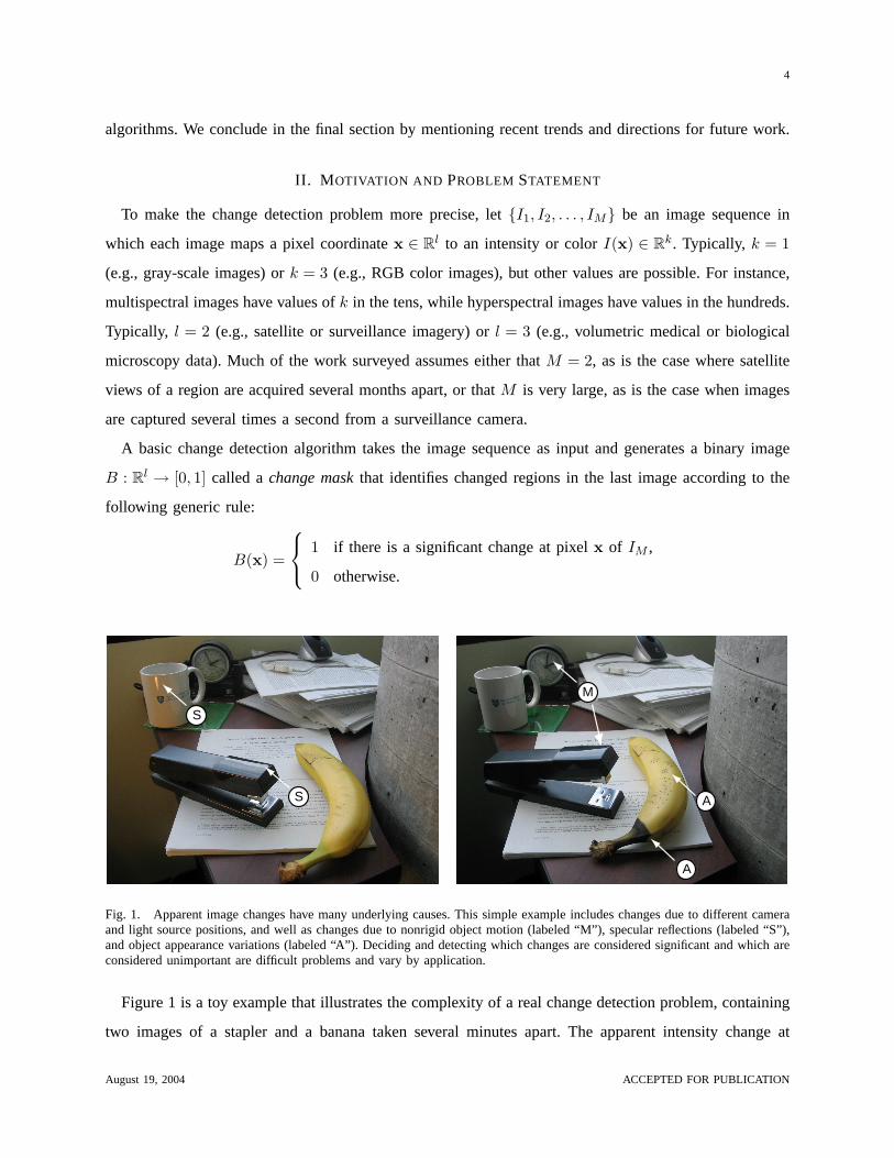
Fig. 1. Apparent image changes have many underlying causes. This simple example includes changes due to different cameraand light source positions, and well as changes due to nonrigid object motion (labeled “M”), specular reflections (labeled “S”),and object appearance variations (labeled “A”). Deciding and detecting which changes are considered significant and which areconsidered unimportant are difficult problems and vary by application.

Figure 1 is a toy example that illustrates the complexity of a real change detection problem, containing

two images of a stapler and a banana taken several minutes apart. The apparent intensity change at


5

V I

A

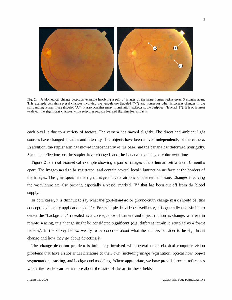
Fig. 2. A biomedical change detection example involving a pair of images of the same human retina taken 6 months apart.This example contains several changes involving the vasculature (labeled “V”) and numerous other important changes in thesurrounding retinal tissue (labeled “A”). It also contains many illumination artifacts at the periphery (labeled “I”). It is of interestto detect the significant changes while rejecting registration and illumination artifacts.

each pixel is due to a variety of factors. The camera has moved slightly. The direct and ambient light

sources have changed position and intensity. The objects have been moved independently of the camera.

In addition, the stapler arm has moved independently of the base, and the banana has deformed nonrigidly.

Specular reflections on the stapler have changed, and the banana has changed color over time.

Figure 2 is a real biomedical example showing a pair of images of the human retina taken 6 months

apart. The images need to be registered, and contain several local illumination artifacts at the borders of

the images. The gray spots in the right image indicate atrophy of the retinal tissue. Changes involving

the vasculature are also present, especially a vessel marked “V” that has been cut off from the blood

supply.

In both cases, it is difficult to say what the gold-standard or ground-truth change mask should be; this

concept is generally application-specific. For example, in video surveillance, it is generally undesirable to

detect the “background” revealed as a consequence of camera and object motion as change, whereas in

remote sensing, this change might be considered significant (e.g. different terrain is revealed as a forest

recedes). In the survey below, we try to be concrete about what the authors consider to be significant

change and how they go about detecting it.

The change detection problem is intimately involved with several other classical computer vision

problems that have a substantial literature of their own, including image registration, optical flow, object

segmentation, tracking, and background modeling. Where appropriate, we have provided recent references

where the reader can learn more about the state of the art in these fields.


6

III. PRE-PROCESSINGMETHODS

The goal of a change detection algorithm is to detect “significant” changes while rejecting “unimpor-

tant” ones. Sophisticated methods for making this distinction require detailed modeling of all the expected

types of changes (important and unimportant) for a given application, and integration of these models

into an effective algorithm. The following subsections describe pre-processing steps used to suppress or

filter out common types of “unimportant” changes before making the change detection decision. These

steps generally involve geometric and radiometric (i.e., intensity) adjustments.

A. Geometric Adjustments

Apparent intensity changes at a pixel resulting from camera motion alone are virtually never desired to

be detected as real changes. Hence, a necessary pre-processing step for all change detection algorithms

is accurateimage registration, the alignment of several images into the same coordinate frame.

When the scenes of interest are mostly rigid in nature and the camera motion is small, registration can

often be performed using low-dimensional spatial transformations such as similarity, affine, or projective

transformations. This estimation problem has been well-studied, and several excellent surveys [27], [28],

[29], [30], and software implementations (e.g., the Insight toolkit [31]) are available, so we do not detail

registration algorithms here. Rather, we note some of the issues that are important from a change detection

standpoint.

Choosing an appropriate spatial transformation is critical for good change detection. An excellent

example is registration of curved human retinal images [32], for which an affine transformation is

inadequate but a 12-parameter quadratic model suffices. Several modern registration algorithms are

capable of switching automatically to higher-order transformations after being initialized with a low-

order similarity transformation [33]. In some scenarios (e.g. when the cameras that produced the images

have widely-spaced optical centers, or when the scene consists of deformable/articulated objects) a non-

global transformation may need to be estimated to determine corresponding points between two images,

e.g. via optical flow [34], tracking [35], object recognition and pose estimation [36], [37], or structure-

from-motion [38], [39] algorithms.2

Another practical issue regarding registration is the selection of feature-based, intensity-based or hybrid

registration algorithms. In particular, when feature-based algorithms are used, the accuracy of the features

themselves must be considered in addition to the accuracy of the registration algorithm. One must

2We note that these non-global processes are ordinarily not referred to as “registration” in the literature.


7

consider the possibility of localized registration errors that can result in false change detection, even

when average/global error measures appear to be modest.

Several researchers have studied the effects of registration errors on change detection, especially in the

context of remote sensing [40], [41]. Dai and Khorram [42] progressively translated one multispectral

image against itself and analyzed the sensitivity of a difference-based change detection algorithm (see

Section IV). They concluded that highly accurate registration was required to obtain good change detection

results (e.g. one-fifth-pixel registration accuracy to obtain change detection error of less than 10%).

Bruzzone and Cossu [43] did a similar experiment on two-channel images, and obtained a nonparametric

density estimate of registration noise over the space of change vectors. They then developed a change-

detection strategy that incorporated thisa priori probability that change at a pixel was due to registration

noise.

B. Radiometric/Intensity Adjustments

In several change detection scenarios (e.g. surveillance), intensity variations in images caused by

changes in the strength or position of light sources in the scene are considered unimportant. Even in cases

where there are no actual light sources involved, there may be physical effects with similar consequences

on the image (e.g. calibration errors and variations in imaging system components in magnetic resonance

and computed tomography imagery). In this section, we describe several techniques that attempt to pre-

compensate for illumination variations between images. Alternately, some change detection algorithms

are designed to cope with illumination variation without explicit pre-processing; see Section VII.

1) Intensity Normalization:Some of the earliest attempts at illumination-invariant change detection

used intensity normalization [44], [45], and it is still used [42]. The pixel intensity values in one image

are normalized to have the same mean and variance as those in another, i.e.,

I2(x) =σ1

σ2I2(x)− µ2+ µ1, (1)

whereI2 is the normalized second image andµi, σi are the mean and standard deviation of the intensity

values ofIi, respectively. Alternatively, both images can be normalized to have zero mean and unit

variance. This allows the use of decision thresholds that are independent of the original intensity values

of the images.

Instead of applying the normalization (1) to each pixel using the global statisticsµi, σi, the images

can be divided into corresponding disjoint blocks, and the normalization independently performed using


8

the local statistics of each block. This can achieve better local performance at the expense of introducing

blocking artifacts.

2) Homomorphic Filtering:For images of scenes containing Lambertian surfaces, the observed image

intensity at a pixelx can be modeled as the product of two components: the illuminationIl(x) from the

light source(s) in the scene and the reflectanceIo(x) of the object surface to whichx belongs:

I(x) = Il(x)Io(x). (2)

This is called theshading model[46]. Only the reflectance componentIo(x) contains information about

the objects in the scene. A type of illumination-invariant change detection can hence be performed by

first filtering out the illumination component from the image. If the illumination due to the light sources

Il(x) has lower spatial frequency content than the reflectance componentIo(x), a homomorphic filter

can be used to separate the two components of the intensity signal. That is, logarithms are taken on both

sides of (2) to obtain

ln I(x) = ln Il(x) + ln Io(x).

Since the lower frequency componentln Il(x) is now additive, it can be separated using a high pass

filter. The reflectance component can thus be estimated as

Io(x) = expF (ln I(x)),

whereF (·) is a high pass filter. The reflectance component can be provided as input to the decision rule

step of a change detection process (see, e.g. [47], [48]).

3) Illumination Modeling: Modeling and compensating for local radiometric variation that deviates

from the Lambertian assumption is necessary in several applications (e.g. underwater imagery [49]). For

example, Can and Singh [50] modeled the illumination component as a piecewise polynomial function.

Negahdaripour [51] proposed a generic linear model for radiometric variation between images of the

same scene:

I2(x, y) = M(x, y)I1(x, y) + A(x, y),

whereM(x, y) andA(x, y) are piecewise smooth functions with discontinuities near region boundaries.

Hager and Belhumeur [52] used principal component analysis (PCA) to extract a set of basis images


9

Bk(x, y) that represent the views of a scene under all possible lighting conditions, so that after registration,

I2(x, y) = I1(x, y) +K∑

k=1

αkBk(x, y).

In our experience, these sophisticated models of illumination compensation are not commonly used in the

context of change detection. However, Bromiley et al. [53] proposed several ways that the scattergram,

or joint histogram of image intensities, could be used to estimate and remove a global non-parametric

illumination model from an image pair prior to simple differencing. The idea is related to mutual

information measures used for image registration [54].

4) Linear Transformations of Intensity:In the remote sensing community, it is common to transform

a multispectral image into a different intensity space before proceeding to change detection. For example,

Jensen [55] and Niemeyer et al. [56] discussed applying PCA to the set of all bands from two multispectral

images. The principal component images corresponding to large eigenvalues are assumed to reflect the

unchanged part of the images, and those corresponding to smaller eigenvalues to changed parts of the

images. The difficulty with this approach is determining which of the principal components represent

change without visual inspection. Alternately, one can apply PCA to difference images as in Gong [57],

in which case the first one or two principal component images are assumed to represent changed regions.

Another linear transformation for change detection in remote sensing applications using Landsat data

is the Kauth-Thomas or “Tasseled Cap” transform [58]. The transformed intensity axes are linear combi-

nations of the original Landsat bands and have semantic descriptions including “soil brightness”, “green

vegetation”, and “yellow stuff”. Collins and Woodcock [5] compared different linear transformations of

multispectral intensities for mapping forest changes using Landsat data. Morisette and Khorram [59]

discussed how both an optimal combination of multispectral bands and corresponding decision threshold

to discriminate change could be estimated using a neural network from training data regions labeled as

change/no-change.

In surveillance applications, Elgammal et al. [60] observed that the coordinates( GR+G+B , B

R+G+B , R+

G + B) are more effective than RGB coordinates for suppressing unwanted changes due to shadows of

objects.

5) Sudden Changes in Illumination:Xie et al. [61] observed that under the Phong shading model with

slowly spatially varying illumination, the sign of the difference between corresponding pixel measurements

is invariant to sudden changes in illumination. They used this result to create a change detection algorithm

that is able to discriminate between “uninteresting” changes caused by a sudden change in illumination


10

(e.g. turning on a light switch) and “interesting” changes caused by object motion. See also the background

modeling techniques discussed in Section VIII.

Watanabe et al. [21] discussed an interesting radiometric pre-processing step specifically for change

detection applied to overhead imagery of buildings. Using the known position of the sun and a method

for fitting building models to images, they were able to remove strong shadows of buildings due to direct

light from the sun, prior to applying a change detection algorithm.

6) Speckle Noise:Speckle is an important type of noise-like artifact found in coherent imagery such as

synthetic aperture radar and ultrasound. There is a sizable body of research (too large to summarize here)

on modeling and suppression of speckle (for example, see [62], [63], [64] and the survey by Touzi [65]).

Common approaches to suppressing false changes due to speckle include frame averaging (assuming

speckle is uncorrelated between successive images), local spatial averaging (albeit at the expense of

spatial resolution), thresholding, and statistical model-based and/or multi-scale filtering.

IV. SIMPLE DIFFERENCING

Early change detection methods were based on the signed difference imageD(x) = I2(x)−I1(x), and

such approaches are still widespread. The most obvious algorithm is to simply threshold the difference

image. That is, the change maskB(x) is generated according to the following decision rule:

B(x) =

1 if |D(x)| > τ

0 otherwise,

We denote this algorithm as “simple differencing”. Often the thresholdτ is chosen empirically. Rosin [66],

[67] surveyed and reported experiments on many different criteria for choosingτ . Smits and Annoni [68]

discussed how the threshold can be chosen to achieve application-specific requirements for false alarms

and misses (i.e. the choice of point on a receiver-operating-characteristics curve [69]; see Section X).

There are several methods that are closely related to simple differencing. For example, inchange vector

analysis(CVA) [4], [70], [71], [72], often used for multispectral images, a feature vector is generated for

each pixel in the image, considering several spectral channels. The modulus of the difference between the

two feature vectors at each pixel gives the values of the “difference image”.3 Image ratioingis another

related technique that uses the ratio, instead of the difference, between the pixel intensities of the two

images [19]. DiStefano et al. [73] performed simple differencing on subsampledgradient images. Tests

3In some cases, the direction of this vector can also be used to discriminate between different types of changes [43].


11

that have similar functional forms but are more well-defended from a theoretical perspective are discussed

further in Sections VI and VII below.

However the threshold is chosen, simple differencing with a global threshold is unlikely to outperform

the more advanced algorithms discussed below in any real-world application. This technique is sensitive

to noise and variations in illumination, and does not consider local consistency properties of the change

mask.

V. SIGNIFICANCE AND HYPOTHESISTESTS

The decision rule in many change detection algorithms is cast as a statistical hypothesis test. The

decision as to whether or not a change has occurred at a given pixelx corresponds to choosing one of

two competing hypotheses: thenull hypothesisH0 or the alternative hypothesisH1, corresponding to

no-changeandchangedecisions, respectively.

The image pair(I1(x), I2(x)) is viewed as a random vector. Knowledge of the conditional joint

probability density functions (pdfs)p(I1(x), I2(x)|H0) andp(I1(x), I2(x)|H1) allows us to choose the

hypothesis that best describes the intensity change atx using the classical framework of hypothesis testing

[69], [74].

Since interesting changes are often associated with localized groups of pixels, it is common for the

change decision at a given pixelx to be based on a small block of pixels in the neighborhood ofx in

each of the two images (such approaches are also called “geo-pixel” methods). Alternately, decisions can

be made independently at each pixel and then processed to enforce smooth regions in the change mask;

see Section IX.

We denote a block of pixels centered atx by Ωx. The pixel values in the block are denoted:

I(x) = I(y)|y ∈ Ωx.

Note that I(x) is an ordered set to ensure that corresponding pixels in the image pair are matched

correctly. We assume that the block containsN pixels. There are two methods for dealing with blocks,

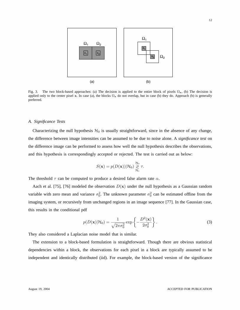
as illustrated in Figure 3. One option is to apply the decision reached atx to all the pixels in the block

Ωx (Figure 3a), in which case the blocks do not overlap, the change mask is coarse, and block artifacts

are likely. The other option is to apply the decision only to pixelx (Figure 3b), in which case the blocks

can overlap and there are fewer artifacts; however, this option is computationally more expensive.


12

x1 x2

Ω1 Ω2x1

x2

Ω1

Ω2

(a) (b)

Fig. 3. The two block-based approaches: (a) The decision is applied to the entire block of pixelsΩx, (b) The decision isapplied only to the center pixelx. In case (a), the blocksΩx do not overlap, but in case (b) they do. Approach (b) is generallypreferred.

A. Significance Tests

Characterizing the null hypothesisH0 is usually straightforward, since in the absence of any change,

the difference between image intensities can be assumed to be due to noise alone. Asignificance teston

the difference image can be performed to assess how well the null hypothesis describes the observations,

and this hypothesis is correspondingly accepted or rejected. The test is carried out as below:

S(x) = p(D(x))|H0)H0

≷H1

τ.

The thresholdτ can be computed to produce a desired false alarm rateα.

Aach et al. [75], [76] modeled the observationD(x) under the null hypothesis as a Gaussian random

variable with zero mean and varianceσ20. The unknown parameterσ2

0 can be estimated offline from the

imaging system, or recursively from unchanged regions in an image sequence [77]. In the Gaussian case,

this results in the conditional pdf

p(D(x)|H0) =1√2πσ2

0

exp−D2(x)

2σ20

. (3)

They also considered a Laplacian noise model that is similar.

The extension to a block-based formulation is straightforward. Though there are obvious statistical

dependencies within a block, the observations for each pixel in a block are typically assumed to be

independent and identically distributed (iid). For example, the block-based version of the significance


13

test (3) uses the test statistic

p(D(x)|H0) =

(1√2πσ2

0

)N

exp

−∑

y∈ΩxD2(y)

2σ20

=

(1√2πσ2

0

)N

exp−G(x)

2

.

Here G(x) =(∑

y∈ΩxD2(y)

)/σ2

0, which has aχ2 pdf with N degrees of freedom. Tables for the

χ2 distribution can be used to compute the decision threshold for a desired false alarm rate. A similar

computation can be performed when each observation is modelled as an independent Laplacian random

variable.

B. Likelihood Ratio Tests

Characterizing the alternative (change) hypothesisH1 is more challenging, since the observations

consist of change components that are not knowna priori or cannot easily be described by parametric

distributions. When both conditional pdfs are known, alikelihood ratio can be formed as:

L(x) =p(D(x)|H1)p(D(x)|H0)

.

This ratio is compared to a thresholdτ defined as:

τ =P (H0)(C10 − C00)P (H1)(C01 − C11)

,

whereP (Hi) is thea priori probability of hypothesisHi, andCij is the cost associated with making a

decision in favor of hypothesisHi whenHj is true. In particular,C10 is the cost associated with “false

alarms” andC01 is the cost associated with “misses”. If the likelihood ratio atx exceedsτ , a decision is

made in favor of hypothesisH1; otherwise, a decision is made in favor of hypothesisH0. This procedure

yields the minimumBayes riskby choosing the hypothesis that has the maximuma posterioriprobability

of having occurred given the observations(I1(x), I2(x)).

Aach et al. [75], [76] characterized both hypotheses by modelling the observations comprisingD(x)

underHi as iid zero-mean Gaussian random variables with varianceσ2i . In this case, the block-based

likelihood ratio is given by:

p(D(x)|H1)p(D(x)|H0)

=σN

0

σN1

exp

− ∑y∈Ωx

D2(y)(

12σ2

1

− 12σ2

0

) .


14

The parametersσ20 and σ2

1 were estimated from unchanged (i.e. very smallD(x)) and changed (i.e.

very largeD(x)) regions of the difference image respectively. As before, they also considered a similar

Laplacian noise model. Rignot and van Zyl [78] described hypothesis tests on the difference and ratio

images from SAR data assuming the true and observed intensities were related by a gamma distribution.

Bruzzone and Prieto [70] noted that while the variances estimated as above may serve as good initial

guesses, using them in a decision rule may result in a false alarm rate different from the desired value.

They proposed an automatic change detection technique that estimates the parameters of the mixture

distributionp(D) consisting of all pixels in the difference image. The mixture distributionp(D) can be

written as:

p(D(x)) = p(D(x)|H0)P (H0) + p(D(x)|H1)P (H1).

The means and variances of the class conditional distributionsp(D(x)|Hi) are estimated using an

expectation-maximization (EM) algorithm [79] initialized in a similar way to the algorithm of Aach

et al. In [4], Bruzzone and Prieto proposed a more general algorithm where the difference image is

initially modelled as a mixture of two nonparametric distributions obtained by the reduced Parzen estimate

procedure [80]. These nonparametric estimates are iteratively improved using an EM algorithm. We

note that these methods can be viewed as a precursor to the more sophisticated background modeling

approaches described in Section VIII.

C. Probabilistic Mixture Models

This category is best illustrated by Black et al. [81], who described an innovative approach to estimating

changes. Instead of classifying the pixels as change/no-change as above, or as object/background as in

Section VIII, they are softly classified into mixture components corresponding to different generative

models of change. These models included (1) parametric object or camera motion, (2) illumination

phenomena, (3) specular reflections and (4) “iconic/pictorial changes” in objects such as an eye blinking

or a nonrigid object deforming (using a generative model learned from training data). A fifth outlier

class collects pixels poorly explained by any of the four generative models. The algorithm operates on

the optical flow field between an image pair, and uses the EM algorithm to perform a soft assignment

of each vector in the flow field to the various classes. The approach is notable in that image registration

and illumination variation parameters are estimated in-line with the changes, instead of beforehand. This

approach is quite powerful, capturing multiple object motions, shadows, specularities, and deformable

models in a single framework.


15

D. Minimum Description Length

To conclude this section, we note that Leclerc et al. [82] proposed a change detection algorithm based

on a concept called “self-consistency” between viewpoints of a scene. The algorithm involves both raw

images and three-dimensional terrain models, so it is not directly comparable to the methods surveyed

above; the main goal of the work is to provide a framework for measuring the performance of stereo

algorithms. However, a notable feature of this approach is its use of the minimum description length

(MDL) model selection principle [83] to classify unchanged and changed regions, as opposed to the

Bayesian approaches discussed earlier. The MDL principle selects the hypothesisHi that more concisely

describes (i.e. using a smaller number of bits) the observed pair of images. We believe MDL-based

model selection approaches have great potential for “standard” image change-detection problems, and

are worthy of further study.

VI. PREDICTIVE MODELS

More sophisticated change detection algorithms result from exploiting the close relationships between

nearby pixels both in space and time (when an image sequence is available).

A. Spatial Models

A classical approach to change detection is to fit the intensity values of each block to a polynomial

function of the pixel coordinatesx. In two dimensions, this corresponds to

Ik(x, y) =p∑

i=0

p−i∑j=0

βkijx

iyj , (4)

where p is the order of the polynomial model. Hsu et al. [84] discussed generalized likelihood ratio

tests using a constant, linear, or quadratic model for image blocks. The null hypothesis in the test is that

corresponding blocks in the two images are best fit by the same polynomial coefficientsβ0ij , whereas the

alternative hypothesis is that the corresponding blocks are best fit by different polynomial coefficients

(β1ij , β

2ij). In each case, the various model parametersβk

ij are obtained by a least-squares fit to the intensity

values in one or both corresponding image blocks. The likelihood ratio is obtained based on derivations

by Yakimovsky [85] and is expressed as:

F (x) =σ2N

0

σN1 σN

2

,

whereN is the number of pixels in the block,σ21 is the variance of the residuals from the polynomial fit

to the block inI1, σ22 is the variance of the residuals from the polynomial fit to the block inI2, andσ2

0


16

is the variance of the residuals from the polynomial fit to both blocks simultaneously. The threshold in

the generalized likelihood ratio test can be obtained using thet-test (for a constant model) or theF -test

(for linear and quadratic models). Hsu et al. used these three models to detect changes between a pair of

surveillance images and concluded that the quadratic model outperformed the other two models, yielding

similar change detection results but with higher confidence.

Skifstad and Jain [86] suggested an extension of Hsu’s intensity modelling technique to make it

illumination-invariant. The authors suggested a test statistic that involved spatial partial derivatives of

Hsu’s quadratic model, given by:

T (x) =∑y∈Ωx

(∂I1

∂x(y)− ∂I2

∂x(y) +

∂I1

∂y(y)− ∂I2

∂y(y)

). (5)

Here, the intensity valuesIj(x) are modelled as quadratic functions of the pixel coordinates (i.e. (4) with

p = 2). The test statistic is compared to an empirical threshold to classify pixels as changed or unchanged.

Since the test statistic only involves partial derivatives, it is independent of linear variations in intensity.

As with homomorphic filtering, the implicit assumption is that illumination variations occur at lower

spatial frequencies than changes in the objects. It is also assumed that true changes in image objects will

be reflected by different coefficients in the quadratic terms that are preserved by the derivative.

B. Temporal Models

When the change detection problem occurs in the context of an image sequence, it is natural to exploit

the temporal consistency of pixels in the same location at different times.

Many authors have modeled pixel intensities over time as an autoregressive (AR) process. An early

reference is Elfishawy et al. [87]. More recently, Jain and Chau [88] assumed each pixel was identically

and independently distributed according to the same (time-varying) Gaussian distribution related to the

past by the same (time-varying) AR(1) coefficient. Under these assumptions, they derived maximum

likelihood estimates of the mean, variance, and correlation coefficient at each point in time, and used

these in likelihood ratio tests where the null (no-change) hypothesis is that the image intensities are

dependent, and the alternate (change) hypothesis is that the image intensities are independent. (This is

similar to Yakimovsky’s hypothesis test above.)

Similarly, Toyama et al. [89] described an algorithm called Wallflower that used a Wiener filter to

predict a pixel’s current value from a linear combination of itsk previous values. Pixels whose prediction

error is several times worse than the expected error are classified as changed pixels. The predictive


17

coefficients are adpatively updated at each frame. This can also be thought of as a background estimation

algorithm; see Section VIII. The Wallflower algorithm also tries to correctly classify the interiors of

homogeneously colored, moving objects by determining the histogram of connected components of change

pixels and adding pixels to the change mask based on distance and color similarity. Morisette and

Khorram’s work [59], discussed in Section III-B.4, can be viewed as a supervised method to determine

an optimal linear predictor.

Carlotto [90] claimed that linear models perform poorly, and suggested a nonlinear dependence to model

the relationship between two images in a sequenceIi(x) andIj(x) under the no-change hypothesis. The

optimal nonlinear function is simplyfij , the conditional expected value of the intensityIi(x) givenIj(x).

For anN -image sequence, there areN(N − 1)/2 total residual error images:

εij(x, y) = [Ii(x, y)− fij(Ij(x))]− [Ij(x, y)− fji(Ii(x))].

These images are then thresholded to produce binary change masks. Carlotto went on to detect specific

temporal patterns of change by matching the string ofN binary change decisions at a pixel with a desired

input pattern.

Clifton [91] used an adaptive neural network to identify small-scale changes from a sequence of

overhead multispectral imagery. This can be viewed as an unsupervised method for learning the parameters

of a nonlinear predictor. Pixels for which the predictor performs poorly are classified as changed. The

goal is to distinguish “unusual” changes from “expected” changes, but this terminology is somewhat

vague does not seem to correspond directly to the notions of “foreground” and “background” in Section

VIII.

VII. T HE SHADING MODEL

Several change detection techniques are based on the shading model for the intensity at a pixel as

described in Section III-B.2 to produce an algorithm that is said to be illumination-invariant. Such

algorithms generally compare the ratio of image intensities

R(x) =I2(x)I1(x)

.

to a threshold determined empirically. We now show the rationale for this approach.

Assuming shading models for the intensitiesI1(x) andI2(x), we can writeI1(x) = Il1(x)Io1(x) and


18

I2(x) = Il2(x)Io2(x), which implies

I2(x)I1(x)

=Il2(x)Io2(x)Il1(x)Io1(x)

. (6)

Since the reflectance componentIoi(x) depends only on the intrinsic properties of the object surface

imaged atx, Io1(x) = Io2(x) in the absence of a change. This observation simplifies (6) to:

I2(x)I1(x)

=Il2(x)Il1(x)

.

Hence, if the illuminationsIl1 andIl2 in each image are approximated as constant within a blockΩx,

the ratio of intensitiesI2(x)/I1(x) remains constant under the null hypothesisH0. This justifies a null

hypothesis that assumes linear dependence between vectors of corresponding pixel intensities, giving rise

to the test statisticR(x).

Skifstad and Jain [86] suggested the following method to assess the linear dependence between two

blocks of pixel valuesI1(x) and I2(x): construct

η(x) =1N

∑y∈Ωx

(R(x)− µx)2 , (7)

whereµx is given by:

µx =1N

∑y∈Ωx

R(x).

When η(x) exceeds a threshold, a decision is made in favor of a change. The linear dependence

detector (LDD) proposed by Durucan and Ebrahimi [92], [93] is closely related to the shading model in

both theory and implementation, mainly differing in the form of the linear dependence test (e.g. using

determinants of Wronskian or Grammian matrices [94]).

Mester, Aach and others [48], [95] criticized the test criterion (7) asad hoc, and expressed the

linear dependence model using a different hypothesis test. Under the null hypothesisH0, each image is

assumed to be a function of a noise-free underlying imageI(x). The vectors of image intensities from

correspondingN -pixel blocks centered atx under the null hypothesisH0 are expressed as:

I1(x) = I(x) + δ1;

I2(x) = kI(x) + δ2.

Here,k is an unknown scaling constant representing the illumination, andδ1, δ2 are two realizations of a

noise block in which each element is iidN (0, σ2n). The projection ofI2(x) onto the subspace orthogonal


19

to I1(x) is given by:

O(x) = I2(x)−

(I1(x)T I2(x)‖I1(x)‖2

)I1(x).

This is zero if and only ifI1(x) and I2(x) are linearly dependent. The authors showed that in an

appropriate basis, the joint pdf of the projectionO(x) under the null hypothesisH0 is approximately a

χ2 distribution withN − 1 degrees of freedom, and used this result both for significance and likelihood

ratio tests.

Li and Leung [96] also proposed a change detection algorithm involving the shading model, using a

weighted combination of the intensity difference and a texture difference measure involving the intensity

ratio. The texture information is assumed to be less sensitive to illumination variations than the raw

intensity difference. However, in homogeneous regions, the texture information becomes less valid and

more weight is given to the intensity difference.

Liu et al. [97] suggested another change detection scheme that uses a significance test based on the

shading model. The authors compared circular shift moments to detect changes instead of intensity ratios.

These moments are designed to represent the reflectance component of the image intensity, regardless

of illumination. The authors claimed that circular shift moments capture image object details better than

the second-order statistics used in (7), and derived a set of iterative formulas to calculate the moments

efficiently.

VIII. B ACKGROUND MODELING

In the context of surveillance applications, change detection is closely related to the well-studied

problem of background modeling. The goal is to determine which pixels belong to the background,

often prior to classifying the remaining foreground pixels (i.e. changed pixels) into different object

classes.4 Here, the change detection problem is qualitatively much different than in typical remote sensing

applications. A large amount of frame-rate video data is available, and the images between which it is

desired to detect changes are spaced apart by seconds rather than months. The entire image sequence is

used as the basis for making decisions about change, as opposed to a single image pair. Furthermore,

there is frequently an important semantic interpretation to the change that can be exploited (e.g. a person

enters a room, a delivery truck drives down a street).

4It is sometimes difficult to rigorously define what is meant by these terms. For example, a person may walk into a room andfall asleep in a chair. At what point does the motionless person transition from foreground to background?


20

Several approaches to background modeling and subtraction were recently collected in a special issue

of IEEE PAMI on video surveillance [1]. The reader is also referred to the results from the DARPA

VSAM (Visual Surveillance and Monitoring) project at Carnegie Mellon University [98] and elsewhere.

Most background modeling approaches assume the camera is fixed, meaning the images are already

registered (though see the last paragraph in this section). Toyama et al. [89] gave a good overview of

several background maintenance algorithms and provided a comparative example.

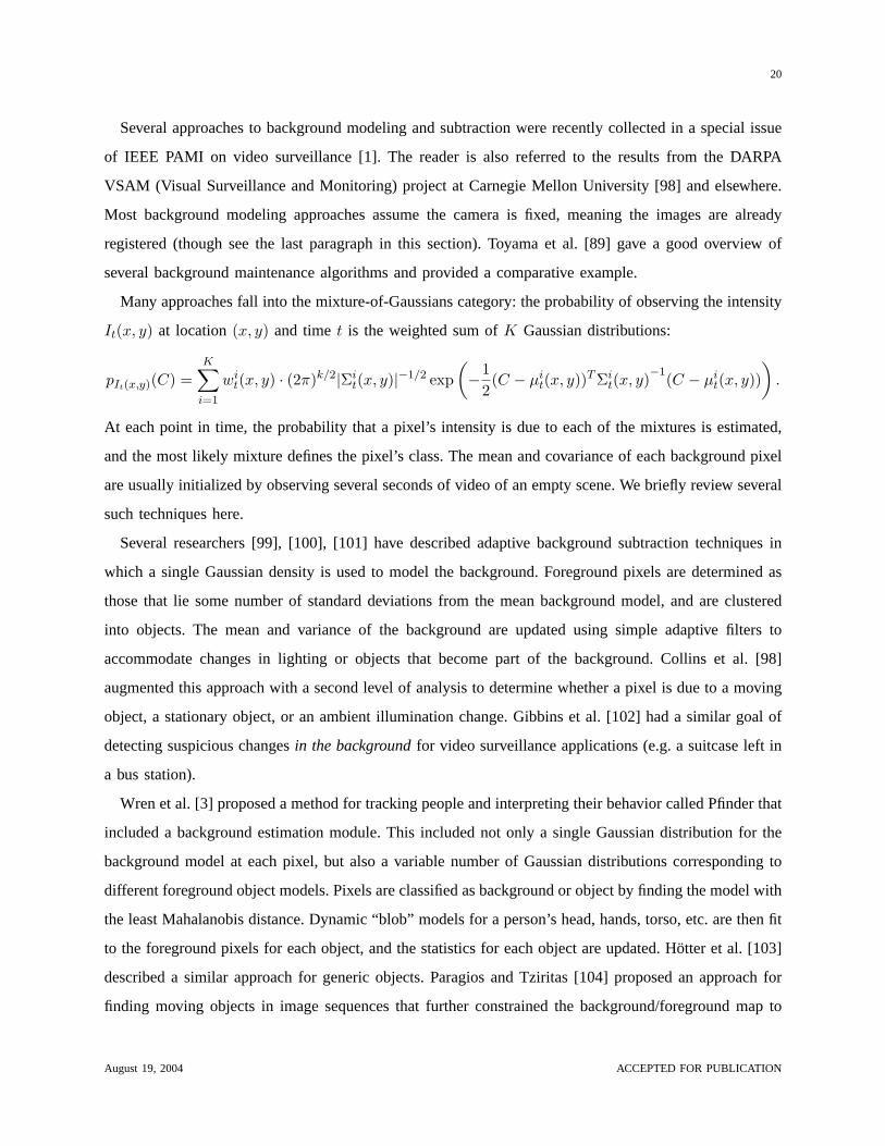
Many approaches fall into the mixture-of-Gaussians category: the probability of observing the intensity

It(x, y) at location(x, y) and timet is the weighted sum ofK Gaussian distributions:

pIt(x,y)(C) =K∑

i=1

wit(x, y) · (2π)k/2|Σi

t(x, y)|−1/2 exp(−1

2(C − µi

t(x, y))T Σit(x, y)−1(C − µi

t(x, y)))

.

At each point in time, the probability that a pixel’s intensity is due to each of the mixtures is estimated,

and the most likely mixture defines the pixel’s class. The mean and covariance of each background pixel

are usually initialized by observing several seconds of video of an empty scene. We briefly review several

such techniques here.

Several researchers [99], [100], [101] have described adaptive background subtraction techniques in

which a single Gaussian density is used to model the background. Foreground pixels are determined as

those that lie some number of standard deviations from the mean background model, and are clustered

into objects. The mean and variance of the background are updated using simple adaptive filters to

accommodate changes in lighting or objects that become part of the background. Collins et al. [98]

augmented this approach with a second level of analysis to determine whether a pixel is due to a moving

object, a stationary object, or an ambient illumination change. Gibbins et al. [102] had a similar goal of

detecting suspicious changesin the backgroundfor video surveillance applications (e.g. a suitcase left in

a bus station).

Wren et al. [3] proposed a method for tracking people and interpreting their behavior called Pfinder that

included a background estimation module. This included not only a single Gaussian distribution for the

background model at each pixel, but also a variable number of Gaussian distributions corresponding to

different foreground object models. Pixels are classified as background or object by finding the model with

the least Mahalanobis distance. Dynamic “blob” models for a person’s head, hands, torso, etc. are then fit

to the foreground pixels for each object, and the statistics for each object are updated. Hotter et al. [103]

described a similar approach for generic objects. Paragios and Tziritas [104] proposed an approach for

finding moving objects in image sequences that further constrained the background/foreground map to


21

be a Markov Random Field (see Section IX below).

Stauffer and Grimson [2] extended the multiple object model above to also allow the background model

to be a mixture of several Gaussians. The idea is to correctly classifydynamicbackground pixels, such

as the swaying branches of a tree or the ripples of water on a lake. Every pixel value is compared against

the existing set of models at that location to find a match. The parameters for the matched model are

updated based on a learning factor. If there is no match, the least-likely model is discarded and replaced

by a new Gaussian with statistics initialized by the current pixel value. The models that account for some

predefined fraction of the recent data are deemed “background” and the rest “foreground”. There are

additional steps to cluster and classify foreground pixels into semantic objects and track the objects over

time.

The Wallflower algorithm by Toyama et al. [89] described in Section VI also includes a frame-level

background maintenance algorithm. The intent is to cope with situations where the intensities of most

pixels change simultaneously, e.g. as the result of turning on a light. A “representative set” of background

models is learned via k-means clustering during a training phase. The best background model is chosen

on-line as the one that produces the lowest number of foreground pixels. Hidden Markov Models can be

used to further constrain the transitions between different models at each pixel [105], [106].

Haritaoglu et al. [107] described a background estimation algorithm as part of theirW 4 tracking

system. Instead of modeling each pixel’s intensity by a Gaussian, they analyzed a video segment of the

empty background to determine the minimum (m) and maximum (M ) intensity values as well as the

largest interframe difference (δ). If the observed pixel is more thanδ levels away from eitherm or M ,

it is considered foreground.

Instead of using Gaussian densities, Elgammal et al. [60] used a non-parametric kernel density estimate

for the intensity of the background and each foreground object. That is,

pIt(x,y)(C) =1N

N∑i=1

Kσ(C − It−i(x, y)),

whereKσ is a kernel function with bandwidthσ. Pixel intensities that are unlikely based on the instan-

taneous density estimate are classified as foreground. An additional step that allows for small deviations

in object position (i.e. by comparingIt(x, y) against the learned densities in a small neighborhood of

(x, y)) is used to suppress false alarms.

Ivanov et al. [108] described a method for background subtraction using multiple fixed cameras. A

disparity map of the empty background is interactively built off-line. On-line, foreground objects are


22

detected as regions where pixels put into correspondence by the learned disparity map have inconsistent

intensities. Latecki et al. [109] discussed a method for semantic change detection in video sequences

(e.g. detecting whether an object enters the frame) using a histogram-based approach that does not

identify which pixels in the image correspond to changes.

Ren et al. [110] extended a statistical background modeling technique to cope with a non-stationary

camera. The current image is registered to the estimated background image using an affine or projective

transformation. A mixture-of-Gaussians approach is then used to segment foreground objects from the

background. Collins et al. [98] also discussed a background subtraction routine for a panning and

tilting camera whereby the current image is registered using a projective transformation to one of many

background images collected off-line.

We stop at this point, though the discussion could range into many broad, widely studied computer

vision topics such as segmentation [111], [112], tracking [35], and layered motion estimation [113], [114].

IX. CHANGE MASK CONSISTENCY

The output of a change detection algorithm where decisions are made independently at each pixel will

generally be noisy, with isolated change pixels, holes in the middle of connected change components,

and jagged boundaries. Since changes in real image sequences often arise from the appearance or motion

of solid objects in a specific size range with continuous, differentiable boundaries, most change detection

algorithms try to conform the change mask to these expectations.

The simplest techniques simply postprocess the change mask with standard binary image processing

operations, such as median filters to remove small groups of pixels that differ from their neighbors’ labels

(salt and pepper noise) [115] or morphological operations [116] to smooth object boundaries.

Such approaches are less optimal than those that enforce spatial priors in the process of constructing

the change mask. For example, Yamamoto [117] described a method in which an image sequence

is collected into a three-dimensional stack, and regions of homogeneous intensity are unsupervisedly

clustered. Changes are detected at region boundaries perpendicular to the temporal axis.

Most attempts to enforce consistency in change regions apply concepts from Markov-Gibbs random

fields (MRFs), which are widely used in image segmentation. A standard technique is to apply a Bayesian

approach where the prior probability of a given change mask is

P (B) =1Z

exp−E(B),

whereZ is a normalization constant andE(B) is an energy term that is low when the regions inB


23

exhibit smooth boundaries and high otherwise. For example, Aach et al. choseE(B) to be proportional

to the number of label changes between 4- and 8-connected neighbors inB. They discussed both an

iterative method for a still image pair [75] and a non-iterative method for an image sequence [76] for

Bayesian change detection using such MRF priors. Bruzzone and Prieto [4], [70] used an MRF approach

with a similar energy function. They maximized thea posteriori probability of the change mask using

Besag’s iterated conditional modes algorithm [118].

Instead of using a prior that influences the final change mask to be close to an MRF, Kasetkasem

and Varshney [119] explicitly constrained the output change mask to be a valid MRF. They proposed

a simulated annealing algorithm [120] to search for the globally optimal change mask (i.e. the MAP

estimate). However, they assumed that the inputs themselves were MRFs, which may be a reasonable

assumption in terrain imagery, but less so for indoor surveillance imagery.

Finally, we note that some authors [103], [121] have taken an object-oriented approach to change

detection, in which pixels are unsupervisedly clustered into homogeneously-textured objectsbeforeap-

plying change detection algorithms. More generally, as stated in the introduction, there is a wide range of

algorithms that use prior models for expected objects (e.g. buildings, cars, people) to constrain the form

of the objects in the detected change mask. Such scene understanding methods can be quite powerful,

but are more accurately characterized as model-based segmentation and tracking algorithms than change

detection.

X. PRINCIPLES FORPERFORMANCEEVALUATION AND COMPARISON

The performance of a change detection algorithm can be evaluated visually and quantitatively based

on application needs. Components of change detection algorithms can also be evaluated individually. For

example, Toyama et al. [89] gave a good overview of several background maintenance algorithms and

provided a comparative example.

The most reliable approach for qualitative/visual evaluation is to display a flicker animation [122], a

short movie file containing a registered pair of images(I1(x), I2(x)) that are played in rapid succession at

intervals of about a second each. In the absence of change, one perceives a steady image. When changes

are present, the changed regions appear to flicker. The estimated change mask can also be superimposed

on either image (e.g. as a semitransparent overlay, with different colors for different types of change).

Quantitative evaluation is more challenging, primarily due to the difficulty of establishing a valid

“ground truth,” or “gold standard.” This is the process of establishing the “correct answer” for whatexactly

the algorithm is expected to produce. A secondary challenge with quantitative validation is establishing


24

the relative importance of different types of errors.

Arriving at the ground truth is an image analysis problem that is known to be difficult and time-

consuming [123]. Usually, the most appropriate source for ground truth data is an expert human observer.

For example, a radiologist would be an appropriate expert human observer for algorithms performing

change detection of X-ray images. As noted by Tan et al. [124], multiple expert human observers can

differ considerably even when they are provided with a common set of guidelines. The same human

observer can even generate different segmentations for the same data at two different times.

With the above-noted variability in mind, the algorithm designer may be faced with the need to establish

ground truth from multiple conflicting observers [125]. A conservative method is to compare the algorithm

against the set intersection of all human observers’ segmentations. In other words, a change detected by

the algorithm would be considered valid if every human observer considers it a change. A method that is

less susceptible to a single overly conservative observer is to use a majority rule. The least conservative

approach is to compare the algorithm against the set union of all human observers’ results. Finally, it

is often possible to bring the observers together after an initial blind markup to develop a consensus

markup.

Once a ground truth has been established, there are several standard methods for comparing the ground

truth to a candidate binary change mask. The following quantities are generally involved:

• True positives (TP): the number of change pixels correctly detected;

• False positives (FP): the number of no-change pixels incorrectly detected as change (also known as

false alarms);

• True negatives (TN): the number of no-change pixels correctly detected; and

• False negatives (FN): the number of change pixels incorrectly detected as no-change (also known

as misses).

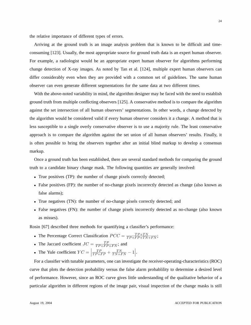
Rosin [67] described three methods for quantifying a classifier’s performance:

• The Percentage Correct ClassificationPCC = TP+TNTP+FP+TN+FN ;

• The Jaccard coefficientJC = TPTP+FP+FN ; and

• The Yule coefficientY C =∣∣∣ TPTP+FP + TN

TN+FN − 1∣∣∣.

For a classifier with tunable parameters, one can investigate the receiver-operating-characteristics (ROC)

curve that plots the detection probability versus the false alarm probablility to determine a desired level

of performance. However, since an ROC curve gives little understanding of the qualitative behavior of a

particular algorithm in different regions of the image pair, visual inspection of the change masks is still


25

recommended.

Finally, we note that when there is an expected semantic interpretation of the changed pixels in a

given application (e.g. an intruder in surveillance imagery), the algorithm designer should incorporate

higher-level constraints that reflect the ability of a given algorithm to detect the “most important” changes,

instead of treating every pixel equally.

XI. CONCLUSIONS ANDDISCUSSION

The two application domains that have seen the most activity in change detection algorithms are

remote sensing and video surveillance, and their approaches to the problem are often quite different. We

have attempted to survey the recent state of the art in image change detection without emphasizing a

particular application area. We hope that our classification of algorithms into a relatively small number

of categories will provide useful guidance to the algorithm designer. We note there are several software

packages that include some of the change detection algorithms discussed here (e.g. [126], [127]). In

particular, we have developed a companion website to this paper [128] that includes implementations,

results, and comparative analysis of several of the methods discussed above.

We have tried not to over-editorialize regarding the relative merits of the algorithms, leaving the reader

to decide which assumptions and constraints may be most relevant for his or her application. However,

our opinion is that two algorithms deserve special mention. Stauffer and Grimson’s background modeling

algorithm [2], covered in Section VIII, provides for multiple models of background appearance as well

as object appearance and motion. The algorithm by Black et al. [81], covered in Section V-C, provides

for multiple models of image change and requires no preprocessing to compensate for misregistration or

illumination variation. We expect that a combination of these approaches that uses soft assignment of

each pixel to an object class and one or more change models would produce a very general, powerful,

and theoretically well-justified change detection algorithm.

Despite the substantial amount of work in the field, change detection is still an active and interesting

area of research. We expect future algorithm developments to be fueled by increasingly more integrated

approaches combining elaborate models of change, implicit pre- and post-processing, robust statistics,

and global optimization methods. We also expect future developments to leverage progress in the related

areas of computer vision research (e.g. segmentation, tracking, motion estimation, structure-from-motion)

mentioned in the text. Finally, and perhaps most importantly, we expect a continued growth of societal

applications of change detection and interpretation in key areas such as biotechnology and geospatial

intelligence.


26

XII. A CKNOWLEDGMENTS

Thanks to the anonymous reviewers and associate editors for their important comments that helped

improve the quality of this work. This work was supported in part by CenSSIS, the Center for Subsurface

Sensing and Imaging Systems, under the Engineering Research Centers Program of the National Science

Foundation (Award Number EEC-9986821). Thanks to Dr. A. Majerovics at the Center for Sight in

Albany, NY for the images in Figure 2.

REFERENCES

[1] R. Collins, A. Lipton, and T. Kanade, “Introduction to the special section on video surveillance,”IEEE Trans. Pattern

Anal. Machine Intell., vol. 22, no. 8, pp. 745–746, August 2000.

[2] C. Stauffer and W. E. L. Grimson, “Learning patterns of activity using real-time tracking,”IEEE Trans. Pattern Anal.

Machine Intell., vol. 22, no. 8, pp. 747–757, August 2000.

[3] C. R. Wren, A. Azarbayejani, T. Darrell, and A. Pentland, “Pfinder: Real-time tracking of the human body,”IEEE Trans.

Pattern Anal. Machine Intell., vol. 19, no. 7, pp. 780–785, 1997.

[4] L. Bruzzone and D. F. Prieto, “An adaptive semiparametric and context-based approach to unsupervised change detection

in multitemporal remote-sensing images,”IEEE Trans. Image Processing, vol. 11, no. 4, pp. 452–466, April 2002.

[5] J. B. Collins and C. E. Woodcock, “An assessment of several linear change detection techniques for mapping forest

mortality using multitemporal Landsat TM data,”Remote Sensing Environment, vol. 56, pp. 66–77, 1996.

[6] A. Huertas and R. Nevatia, “Detecting changes in aerial views of man-made structures,”Image and Vision Computing,

vol. 18, no. 8, pp. 583–596, May 2000.

[7] M. Bosc, F. Heitz, J. P. Armspach, I. Namer, D. Gounot, and L. Rumbach, “Automatic change detection in multimodal

serial MRI: application to multiple sclerosis lesion evolution,”Neuroimage, vol. 20, pp. 643–656, 2003.

[8] M. J. Dumskyj, S. J. Aldington, C. J. Dore, and E. M. Kohner, “The accurate assessment of changes in retinal vessel

diameter using multiple frame electrocardiograph synchronised fundus photography,”Current Eye Research, vol. 15, no. 6,

pp. 652–632, June 1996.

[9] L. Lemieux, U. Wieshmann, N. Moran, D. Fish, , and S. Shorvon, “The detection and significance of subtle changes

in mixed-signal brain lesions by serial MRI scan matching and spatial normalization,”Medical Image Analysis, vol. 2,

no. 3, pp. 227–242, 1998.

[10] D. Rey, G. Subsol, H. Delingette, and N. Ayache, “Automatic detection and segmentation of evolving processes in 3D

medical images: Application to multiple sclerosis,”Medical Image Analysis, vol. 6, no. 2, pp. 163–179, June 2002.

[11] J.-P. Thirion and G. Calmon, “Deformation analysis to detect and quantify active lesions in three-dimensional medical

image sequences,”IEEE Transactions on Medical Image Analysis, vol. 18, no. 5, pp. 429–441, 1999.

[12] E. Landis, E. Nagy, D. Keane, and G. Nagy, “A technique to measure 3D work-of-fracture of concrete in compression,”

J. Engineering Mechanics, vol. 126, no. 6, pp. 599–605, June 1999.

[13] G. Nagy, T. Zhang, W. Franklin, E. Landis, E. Nagy, and D. Keane, “Volume and surface area distributions of cracks in

concrete,” inVisual Form 2001 (Springer LNCS 2059), 2001, pp. 759–768.

[14] D. Edgington, W. Dirk, K. Salamy, C. Koch, M. Risi, and R. Sherlock, “Automated event detection in underwater video,”

in Proc. MTS/IEEE Oceans 2003 Conference, 2003.


27

[15] K. Lebart, E. Trucco, and D. M. Lane, “Real-time automatic sea-floor change detection from video,” inMTS/IEEE

OCEANS 2000, September 2000, pp. 337–343.

[16] J. Whorff and L. Griffing, “A video recording and analysis system used to sample intertidal communities,”Journal of

Experimental Marine Biology and Ecology, vol. 160, pp. 1–12, 1992.

[17] C.-Y. Fang, S.-W. Chen, and C.-S. Fuh, “Automatic change detection of driving environments in a vision-based driver

assistance system,”IEEE Trans. Neural Networks, vol. 14, no. 3, pp. 646–657, May 2003.

[18] W. Y. Kan, J. V. Krogmeier, and P. C. Doerschuk, “Model-based vehicle tracking from image sequences with an application

to road surveillance,”Opt. Eng., vol. 35, no. 6, pp. 1723–1729, 1996.

[19] A. Singh, “Digital change detection techniques using remotely-sensed data,”Internat. Journal of Remote Sensing, vol. 10,

no. 6, pp. 989–1003, 1989.

[20] P. Coppin and M. Bauer, “Digital change detection in forest ecosystems with remote sensing imagery,”Remote Sensing

Reviews, vol. 13, pp. 207–234, 1996.

[21] S. Watanabe, K. Miyajima, and N. Mukawa, “Detecting changes of buildings from aerial images using shadow and

shading model,” inICPR 98, 1998, pp. 1408–1412.

[22] P. Deer and P. Eklund, “Values for the fuzzy C-means classifier in change detection for remote sensing,” inProceedings

of the 9th Int. Conf. on Information Processing and Management of Uncertainty (IPMU 2002), 2002, pp. 187–194.

[23] L. Bruzzone and S. Serpico, “An iterative technique for the detection of land-cover transitions in multitemporal remote-

sensing images,”IEEE Trans. Geosci. Remote Sensing, vol. 35, no. 4, pp. 858–867, July 1997.

[24] F. Gustafsson,Adaptive Filtering and Change Detection. John Wiley & Sons, 2000.

[25] M. Yeung, B. Yeo, and B. Liu, “Segmentation of video by clustering and graph analysis,”Computer Vision and Image

Understanding, vol. 71, no. 1, pp. 94–109, July 1998.

[26] H. Yu and W. Wolf, “A hierarchical multiresolution video shot transition detection scheme,”Computer Vision and Image

Understanding, vol. 75, no. 1/2, pp. 196–213, July 1999.

[27] L. G. Brown, “A survey of image registration techniques,”ACM Computer Surv., vol. 24, no. 4, 1992.

[28] S. Lavallee,Registration for computer-integrated surgery: methodology, state of the art. MIT Press, 1995.

[29] J. B. A. Maintz and M. A. Viergever, “A survey of medical image registration,”Medical Image Analysis, vol. 2, no. 1,

pp. 1–36, 1998.

[30] B. Zitova and J. Flusser, “Image registration methods: a survey,”Image and Vision Computing, vol. 21, pp. 977–1000,

2003.

[31] L. Ibanez, W. Schroeder, L. Ng, and J. Cates,The ITK Software Guide: The Insight Segmentation and Registration Toolkit

(version 1.4). Kitware Inc., 2003.

[32] A. Can, C. V. Stewart, B. Roysam, and H. L. Tanenbaum, “A feature-based robust hierarchical algorithm for registration

pairs of images of the curved human retina,”IEEE Transactions on Pattern Analysis and Machine Intelligence, vol. 24,

no. 3, March 2002.

[33] C. V. Stewart, C.-L. Tsai, and B. Roysam, “A dual bootstrap iterative closest point (icp) algorithm: Application to retinal

image registration,”IEEE Transactions on Medical Imaging - Special Issue on Medical Image Registration, vol. 22,

no. 11, November 2003.

[34] J. Barron, D. Fleet, and S. Beauchemin, “Performance of optical flow techniques,”International Journal of Computer

Vision, vol. 12, no. 1, pp. 43–77, 1994.

[35] A. Blake and M. Isard,Active Contours. Springer Verlag, 1999.


28

[36] D. G. Lowe, “Distinctive image features from scale-invariant keypoints,”International Journal of Computer Vision, 2004,

to appear.

[37] W. Wells, “Statistical approaches to feature-based object recognition,”International Journal of Computer Vision, vol. 21,

no. 1/2, pp. 63–98, 1997.

[38] D. Forsyth and J. Ponce,Computer Vision: A Modern Approach. Prentice Hall, 2003.

[39] R. Hartley and A. Zisserman,Multiple View Geometry in Computer Vision. Cambridge University Press, 2000.

[40] D. A. Stow, “Reducing the effects of misregistration on pixel-level change detection,”Int. J. Remote sensing, vol. 20,

no. 12, pp. 2477–2483, 1999.

[41] J. Townshend, C. Justice, C. Gurney, and J. McManus, “The impact of misregistration on change detection,”IEEE Trans.

Geosci. Remote Sensing, vol. 30, pp. 1054–1060, September 1992.

[42] X. Dai and S. Khorram, “The effects of image misregistration on the accuracy of remotely sensed change detection,”

IEEE Trans. Geoscience and Remote Sensing, vol. 36, no. 5, pp. 1566–1577, September 1998.

[43] L. Bruzzone and R. Cossu, “An adaptive approach to reducing registration noise effects in unsupervised change detection,”

IEEE Trans. Geoscience and Remote Sensing, vol. 41, no. 11, pp. 2455–2465, November 2003.

[44] R. Lillestrand, “Techniques for change detection,”IEEE Trans. on Computers, vol. 21, no. 7, pp. 654–659, 1972.

[45] M. S. Ulstad, “An algorithm for estimating small scale differences between two digital images,”Pattern Recognition,

vol. 5, pp. 323–333, 1973.

[46] B. Phong, “Illumination for computer generated pictures,”Commun. ACM, vol. 18, pp. 311–317, 1975.

[47] T. A. D. Toth and V. Metzler, “Illumination-invariant change detection,” inThe 4th IEEE Southwest Symposium on Image

Analysis and Interpretation, April 2000.

[48] T. Aach, L. Dumbgen, R. Mester, and D. Toth, “Bayesian illumination-invariant motion detection,” inProc. IEEE

International Conference on Image Processing, October 2001, pp. 640–643.

[49] O. Pizarro and H. Singh, “Toward large-area mosaicing for underwater scientific applications,”IEEE Journal of Oceanic

Engineering, vol. 28, no. 4, pp. 651–672, October 2003.

[50] A. Can and H. Singh, “Methods for correcting lighting pattern and attenuation in underwater imagery,”IEEE Journal of

Oceanic Engineering, April 2004, in review.

[51] S. Negahdaripour, “Revised definition of optical flow: integration of radiometric and geometric cues for dynamic scene

analysis,”IEEE Trans. Pattern Anal. Machine Intell., vol. 20, no. 9, pp. 961–979, September 1998.

[52] G. D. Hager and P. N. Belhumeur, “Efficient region tracking with parametric models of geometry and illumination,”IEEE

Trans. Pattern Anal. Machine Intell., vol. 20, no. 10, pp. 1025–1039, 1998.

[53] P. Bromiley, N. Thacker, and P. Courtney, “Non-parametric image subtraction using grey level scattergrams,”Image and

Vision Computing, vol. 20, no. 9-10, pp. 609–617, August 2002.

[54] P. Viola, “Alignment by maximization of mutual information,”International Journal of Computer Vision, vol. 24, no. 2,

pp. 137–154, September 1997.

[55] J. Jensen,Introductory Digital Image Processing, A Remote Sensing Perspective. Prentice Hall, 1996.

[56] I. Niemeyer, M. Canty, and D. Klaus, “Unsupervised change detection techniques using multispectral satellite images,”

in Proc. IEEE International Geoscience and Remote Sensing Symposium, 1999, pp. 327–329.

[57] P. Gong, “Change detection using principal components analysis and fuzzy set theory,”Canadian Journal of Remote

Sensing, vol. 19, January 1993.


29

[58] E. P. Crist and R. C. Cicone, “A physically-based transformation of Thematic Mapper data - the TM tasseled cap,”IEEE

Trans. Geoscience and Remote Sensing, vol. 22, pp. 256–263, 1984.

[59] J. Morisette and S. Khorram, “An introduction to using generalized linear models to enhance satellite-based change

detection,”Proc. IGARSS 1997, vol. 4, pp. 1769–1771, 1997.

[60] A. Elgammal, R. Duraiswami, D. Harwood, and L. S. Davis, “Background and foreground modeling using non-parametric

kernel density estimation for visual surveillance,”Proceedings of the IEEE, vol. 90, no. 7, pp. 1151–1163, July 2002.

[61] B. Xie, V. Ramesh, and T. Boult, “Sudden illumination change detection using order consistency,”Image and Vision

Computing, vol. 22, no. 2, pp. 117–125, February 2004.

[62] L. M. T. Carvalho, L. M. G. Fonseca, F. Murtagh, and J. G. P. W. Clevers, “Digital change detection with the aid of

multi-resolution wavelet analysis,”Int. J. Remote Sensing, vol. 22, no. 18, pp. 3871–3876, 2001.

[63] S. Fukuda and H. Hirosawa., “Suppression of speckle in synthetic aperture radar images using wavelet,”Int. J. Remote

Sensing, vol. 19, no. 3, pp. 507–519, 1998.

[64] S. Quegan and J. Schou, “The principles of polarimetric filtering,” inProc. IGARSS ’97, August 1997, pp. 1041–1043.

[65] R. Touzi, “A review of speckle filtering in the context of estimation theory,”IEEE Trans. Geoscience and Remote Sensing,

vol. 40, no. 11, pp. 2392–2404, November 2002.

[66] P. Rosin, “Thresholding for change detection,”Computer Vision and Image Understanding, vol. 86, no. 2, pp. 79–95,

May 2002.

[67] P. Rosin and E. Ioannidis, “Evaluation of global image thresholding for change detection,”Pattern Recognition Letters,

vol. 24, no. 14, pp. 2345–2356, October 2003.

[68] P. Smits and A. Annoni, “Toward specification-driven change detection,”IEEE Trans. Geoscience and Remote Sensing,

vol. 38, no. 3, pp. 1484–1488, May 2000.

[69] H. V. Poor,An Introduction to Signal Detection and Estimation, 2nd ed. Springer-Verlag, 1994.

[70] L. Bruzzone and D. F. Prieto, “Automatic analysis of the difference image for unsupervised change detection,”IEEE

Trans. on Geosci. Remote Sensing, vol. 38, no. 3, pp. 1171–1182, May 2000.

[71] J. E. Colwell and F. P. Weber, “Forest change detection,” inProc. of the 15th International Symposium on Remote Sensing

of Environment, 1981, pp. 839–852.

[72] W. A. Malila, “Change vector analysis: an approach for detecting forest changes with Landsat,” inProc. of the 6th Annual

Symposium on Machine Processing of Remotely Sensed Data, 1980, pp. 326–335.

[73] L. di Stefano, S. Mattoccia, and M. Mola, “A change-detection algorithm based on structure and colour,” inIEEE

Conference on Advanced Video and Signal-Based Surveillance 2003, 2003, pp. 252–259.

[74] S. M. Kay, Fundamentals of Statistical Signal Processing: Detection Theory. Prentice-Hall, 1993.

[75] T. Aach and A. Kaup, “Statistical model-based change detection in moving video,”Signal Processing, vol. 31, pp. 165–

180, March 1993.

[76] ——, “Bayesian algorithms for adaptive change detection in image sequences using Markov random fields,”Signal

Processing: Image Communication, vol. 7, pp. 147–160, August 1995.

[77] R. Thoma and M. Bierling, “Motion compensating interpolation considering covered and uncovered background,”Signal

Processing: Image Communication, vol. 1, no. 2, pp. 191–212, October 1989.

[78] E. Rignot and J. van Zyl, “Change detection techniques for ERS-1 SAR data,”IEEE Trans. Geosci. Remote Sensing,

vol. 31, no. 4, pp. 896–906, July 1993.


30

[79] A. P. Dempster, N. M. Laird, and D. B. Rubin, “Maximum likelihood from imcomplete data via the EM algorithm,”J.

Royal Statist. Soc., vol. 39, no. 1, pp. 1–38, 1977.

[80] K. Fukunaga and R. Hayes, “The reduced Parzen classifier,”IEEE Trans. Pattern Anal. Machine Intell., vol. 11, April

1989.

[81] M. J. Black, D. J. Fleet, and Y. Yacoob, “Robustly estimating changes in image appearance,”Computer Vision and Image

Understanding, vol. 78, no. 1, pp. 8–31, 2000.

[82] Y. G. Leclerc, Q.-T. Luong, and P. V. Fua, “Self-consistency and MDL: A paradigm for evaluating point-correspondence

algorithms, and its application to detecting changes in surface elevation,”International Journal of Computer Vision,

vol. 51, no. 1, pp. 63–83, January 2003.

[83] J. Rissanen, “Minimum-description-length principle,” inEncyclopedia of Statistical Sciences, 5th ed. John Wiley, 1987,

pp. 523–527.

[84] Y. Z. Hsu, H.-H. Nagel, and G. Reckers, “New likelihood test methods for change detection in image sequences,”Computer

Vision, Graphics, and Image Processing, vol. 26, pp. 73–106, 1984.

[85] Y. Yakimovsky, “Boundary and object detection in real world images,”Journal of the ACM, vol. 23, no. 4, pp. 599–618,

October 1976.

[86] K. Skifstad and R. Jain, “Illumination independent change detection for real world image sequences,”Computer Vision,

Graphics, and Image Processing, vol. 46, no. 3, pp. 387–399, 1989.

[87] A. Elfishawy, S. Kesler, and A. Abutaleb, “Adaptive algorithms for change detection in image sequence,”Signal Processing,

vol. 23, no. 2, pp. 179–191, 1991.

[88] Z. Jain and Y. Chau, “Optimum multisensor data fusion for image change detection,”IEEE Trans. Systems, Man and

Cybernetics, vol. 25, no. 9, pp. 1340–1347, September 1995.

[89] K. Toyama, J. Krumm, B. Brumitt, and B. Meyers, “Wallflower: Principles and practice of background maintenance,” in

Proc. ICCV ’99, 1999, pp. 255–261.

[90] M. Carlotto, “Detection and analysis of change in remotely sensed imagery with application to wide area surveillance,”

IEEE Trans. Image Processing, vol. 6, no. 1, pp. 189–202, January 1997.

[91] C. Clifton, “Change detection in overhead imagery using neural networks,”Applied Intelligence, vol. 18, pp. 215–234,

2003.

[92] E. Durucan and T. Ebrahimi, “Change detection and background extraction by linear algebra,”Proc. of IEEE, vol. 89,

no. 10, pp. 1368–1381, October 2001.

[93] ——, “Change detection by nonlinear Grammian,” inNSIP ’01, September 2001.

[94] H. Anton and C. Rorres,Elementary Linear Algebra. Wiley, 1994.

[95] R. Mester, T. Aach, and L. D umbgen, “Illumination-invariant change detection using a statistical colinearity criterion,”

in Proceedings 23rd DAGM Symposium, September 2001, pp. 170–177.

[96] L. Li and M. K. H. Leung, “Integrating intensity and texture differences for robust change detection,”IEEE Trans. Image

Processing, vol. 11, no. 2, pp. 105–112, February 2002.

[97] S. Liu, C. Fu, and S. Chang, “Statistical change detection with moments under time-varying illumination,”IEEE Trans.

Image Processing, vol. 7, no. 9, pp. 1258–1268, September 1998.

[98] R. Collins, A. Lipton, T. Kanade, H. Fujiyoshi, D. Duggins, Y. Tsin, D. Tolliver, N. Enomoto, and O. Hasegawa, “A

system for video surveillance and monitoring,” Robotics Institute, Carnegie Mellon University, Pittsburgh, PA, Tech. Rep.

CMU-RI-TR-00-12, May 2000.


31

[99] A. Cavallaro and T. Ebrahimi, “Video object extraction based on adaptive background and statistical change detection,”

in Proc. SPIE Visual Communications and Image Processing, January 2001, pp. 465–475.

[100] S. Huwer and H. Niemann, “Adaptive change detection for real-time surveillance applications,” inProc. Visual Surveillance

2000, 2000.

[101] T. Kanade, R. Collins, A. Lipton, P. Burt, and L. Wixson, “Advances in cooperative multi-sensor video surveillance,” in

Proc. of the DARPA Image Understanding Workshop, vol. 1, November 1998, pp. 3–24.

[102] D. Gibbins, N. G.N., and B. M.J., “Detecting suspicious background changes in video surveillance of busy scenes,” in

Proceedings Third IEEE Workshop on Applications in Computer Vision (WACV 1996), December 1996, pp. 22–26.

[103] M. Hotter, R. Mester, and M. Meyer, “Detection of moving objects using a robust displacement estimation including a

statistical error analysis,” inInternational Conference on Pattern Recognition, 1996, pp. 249–255.

[104] N. Paragios and G. Tziritas, “Adaptive detection and localization of moving objects in image sequences,”Signal

Processing: Image Communication, vol. 14, no. 4, pp. 277–296, January 1999.

[105] J. Rittscher, J. Kato, S. Joga, and A. Blake, “A probabilistic background model for tracking,” inProc. 6th ECCV, 2000.

[106] B. Stenger, R. Visvanathan, N. Paragios, F. Coetzee, and J. Buhmann, “Topology free Hidden Markov Models: Applications

to background modeling,” inIEEE International Conference on Computer Vision, July 2001, pp. 294–301.

[107] I. Haritaoglu, D. Harwood, and L. S. Davis, “W4: Real-time surveillance of people and their activities,”IEEE Trans.

Pattern Anal. Machine Intell., vol. 22, no. 8, pp. 809–830, August 2000.

[108] Y. Ivanov, A. Bobick, and J. Liu, “Fast lighting independent background subtraction,”International Journal of Computer

Vision, vol. 37, no. 2, pp. 199–207, June 2000.

[109] L. J. Latecki, X. Wen, and N. Ghubade, “Detection of changes in surveillance videos,” inIEEE Int. Conf. on Advanced

Video and Signal Based Surveillance, July 2003.

[110] Y. Ren, C. Chua, and Y. Ho, “Statistical background modeling for non-stationary camera,”Pattern Recognition Letters,

vol. 24, no. 1-3, pp. 183–196, January 2003.

[111] S. Z. Li, Markov Random Field Modeling in Image Analysis, 2nd ed. Springer-Verlag, 2001.

[112] N. Pal and S. Pal, “A review on image segmentation techniques,”Pattern Recognition, vol. 26, no. 9, pp. 1277–1294,

1993.

[113] S. Ayer and H. Sawhney, “Layered representation of motion video using robust maximum-likelihood estimation of mixture

models and MDL encoding,” inProc. ICCV ’95, June 1995.

[114] J. Wang and E. Adelson, “Representing moving objects with layers,”IEEE Transactions on Image Processing Special

Issue: Image Sequence Compression, vol. 3, no. 5, pp. 625–638, September 1994.

[115] R. M. Haralick and L. G. Shapiro,Computer and Robot Vision. Addison-Wesley, 1992, vol. 1.

[116] E. Stringa, “Morphological change detection algorithms for surveillance applications,” inBritish Machine Vision

Conference, 2000.

[117] T. Yamamoto, H. Hanaizumi, and S. Chino, “A change detection method for remotely sensed multispectral and

multitemporal images using 3-D segmentation,”IEEE Trans. Geoscience and Remote Sensing, vol. 39, no. 5, pp. 976–985,

May 2001.

[118] J. Besag, “On the statistical analysis of dirty pictures,”J. Royal Statist. Soc. B, vol. 48, pp. 259–302, 1986.

[119] T. Kasetkasem and P. Varshney, “An image change detection algorithm based on Markov random field models,”IEEE

Trans. on Geosci. Remote Sensing, vol. 40, no. 8, pp. 1815–1823, August 2002.


32

[120] S. Geman and D. Geman, “Stochastic relaxation, Gibbs distributions, and the Bayesian restoration of images,”IEEE

Trans. Pattern Anal. Mach. Intell., vol. 6, no. 6, pp. 721–741, 1984.

[121] O. Hall and G. Hay, “A multi-scale object-specific approach to digital change detection,”International Journal of Applied

Earth Observation and Geoinformation, vol. 4, no. 4, pp. 311–327, 2003.

[122] J. W. Berger, T. R. Patel, D. S. Shin, J. R. Piltz, and R. A. Stone, “Computerized stereochronoscopy and alteration flicker

to detect optic nerve head contour change,”Ophthalmology, vol. 107, no. 7, July 2000.

[123] J. Hu, R. Kahsi, D. Lopresti, G. Nagy, and G. Wilfong, “Why table ground-truthing is hard,” inProc. Sixth Int. Conf.

Document Analysis and Recognition, 2001, pp. 129–133.

[124] I. L. Tan, R. van Schijndel, F. Fazekas, M. Filippi, P. Freitag, D. H. Miller, T. A. Yousry, P. J. W. Pouwels, H. J. Ader,

and F. Barkhof, “Image registration and subtraction to detect activeT2 lesions in MS: An interobserver study,”J. Neurol,

vol. 249, pp. 767–773, 2002.

[125] K. H. Fritzsche, A. Can, H. Shen, C.-L. Tsai, J. N. Turner, H. L. Tanenbaum, C. V. Stewart, and B. Roysam, “Automated

model-based segmentation, tracing, and analysis of retinal vasculature from digital fundus images,” inAngiography and

Plaque Imaging: Advanced Segmentation Techniques. CRC Press, 2003, pp. 225–297.

[126] Applied Analysis Inc., “Adaptive terrain change analysis (ATCA) software,” Billerica, MA, USA. [Online]. Available:

http://www.discover-aai.com/software/products/ATCA.htm

[127] Research Systems Inc., “Environment for visualizing images (ENVI) software,” 2001, Boulder, CO, USA. [Online].

Available: http://www.rsinc.com/envi/index.cfm

[128] S. Andra and O. Al-Kofahi, “Matlab change detection suite,” 2004, Rensselaer Polytechnic Institute, Troy, NY, USA.

[Online]. Available: http://www.ecse.rpi.edu/censsis/papers/change/


Documents

Image Change Detection Algorithms: A Systematic …rjradke/papers/radketip04.pdf1 Image Change Detection Algorithms: A Systematic Survey Richard J. Radke∗, Srinivas Andra, Omar Al-Kofahi,