Embed Size (px)
Citation preview
International Journal of Computer Applications (0975 – 8887)
Volume 42– No.17, March 2012
8
Image Denoising using Neighbors Variation with Wavelet
S D Ruikar
Research Scholar SGGS IET
Nanded, India
D D Doye Professor E&TC
SGGS IET 2nd line of address
ABSTRACT
The image gets corrupted by Additive White Gaussian Noise
during the process of acquisition, transmission, storage and
retrieval. Denoising refers to suppressing the noise while
retaining the edges and other important detailed structures as
much as possible. This paper presents a general structure of
the recovery of images using a combination of variation
methods and wavelet analysis. The variation formulation of
the problem allows us to build the properties of the recovered
signal directly into the analytical machinery. The efficient
wavelet representation allows us to capture and preserve sharp
features in the signal while it evolves in accordance with the
variation laws. We propose the three different variation model
for removing noise as Horizontal, vertical and Cluster.
Horizontal and Vertical variation model obtained the
threshold at each decomposed level of Wavelet. Cluster
variation model moving mask in different wavelet sub band.
This proposed scheme has better PSNR as compared to other
existing technique.
General Terms
Image Processing
Keywords
Horizontal Variation, Vertical Variation, Cluster Variation,
Wavelet, Noise, etc.
1. INTRODUCTION Image processing is a field that continues to grow, with new
applications being developed at an ever increasing pace; it
includes digital cameras, intelligent traffic monitoring,
handwriting recognition on checks, signature validation and
so on. It is a fascinating and exciting area to be involved in
today with application areas ranging from the entertainment
industry to the space program. One of the most interesting
aspects of this information revolution is the ability to send and
receive complex data that transcends ordinary written text.
Visual information, transmitted in the form of digital images,
has become a major method of communication for the 21st
century. During transmission and acquisition, images are
often corrupted by various noises. The aim of image denoising
is to reduce the noise level while keeping the image features
as much as possible [1] [2]. The image denoising approaches
can put into two broad categories like spatial domain and
frequency domain [3]. In the spatial domain approach the
pixels of an image are manipulated directly, such as median
filter, averaging filter, point processing, Weiner filter, etc [4].
The frequency domain approach is based on modifying the
transformed image such as Fourier transform and Wavelet
transform of an image. One of the widely used techniques is
the wavelet thresholding. This scheme performs on noisy
images as small coefficients in the high frequencies. A
thresholding can be done by setting these small coefficients to
zero; will eliminate much of the noise in the image [5] [6].
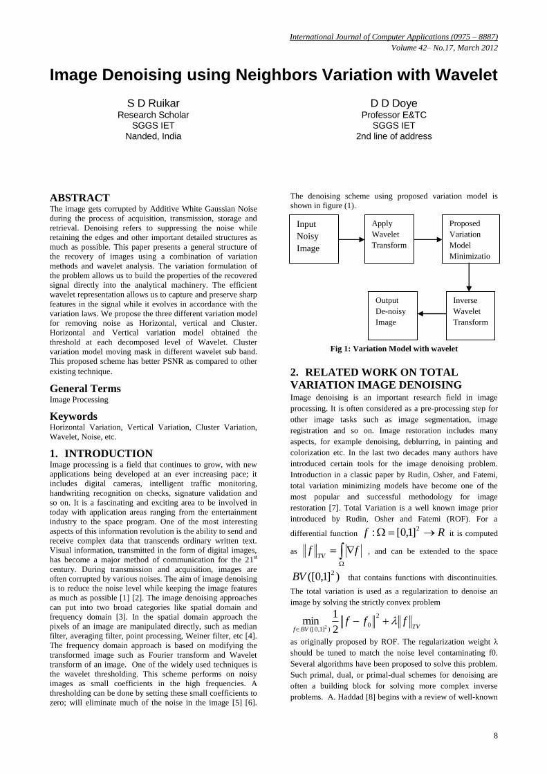
The denoising scheme using proposed variation model is
shown in figure (1).
Fig 1: Variation Model with wavelet
2. RELATED WORK ON TOTAL
VARIATION IMAGE DENOISING Image denoising is an important research field in image
processing. It is often considered as a pre-processing step for
other image tasks such as image segmentation, image
registration and so on. Image restoration includes many
aspects, for example denoising, deblurring, in painting and
colorization etc. In the last two decades many authors have
introduced certain tools for the image denoising problem.
Introduction in a classic paper by Rudin, Osher, and Fatemi,
total variation minimizing models have become one of the
most popular and successful methodology for image
restoration [7]. Total Variation is a well known image prior
introduced by Rudin, Osher and Fatemi (ROF). For a
differential function Rf 2]1,0[: it is computed
as
ffTV
, and can be extended to the space
)]1,0([ 2BV that contains functions with discontinuities.
The total variation is used as a regularization to denoise an
image by solving the strictly convex problem
TVBVffff
2
0)]1,0([ 2
1min
2
as originally proposed by ROF. The regularization weight λ
should be tuned to match the noise level contaminating f0.
Several algorithms have been proposed to solve this problem.
Such primal, dual, or primal-dual schemes for denoising are
often a building block for solving more complex inverse
problems. A. Haddad [8] begins with a review of well-known
Output
De-noisy
Image
Inverse
Wavelet
Transform
Proposed
Variation
Model
Minimizatio
n
Input
Noisy
Image
Apply
Wavelet
Transform
International Journal of Computer Applications (0975 – 8887)
Volume 42– No.17, March 2012
9
properties of BV. They define the space of functions of
bounded variation BV. This space is endowed with an
isotropic norm BV. . They fix the dimension to 2 and
choose 2R so that concentrates on dilatation. S
Osher[9] propose a new model for image restoration and
image decomposition into cartoon and texture, based on the
total variation minimization of Rudin, Osher, and Fatemi, and
on oscillatory functions, which follows results of Meyer[10],
involving H-1 norm. This model performs better on textured
images, and the “residual” component has less structure than
in the standard TV model. Fang fang Dong [11] proposed
vectorial algorithm to some applications besides image
denoising. They stated that vectorial algorithm can be used in
many problems which need the 1l regularization. Yang
Wang and Haomin Zhou [12] propose a denoising algorithm
for medical images based on a combination of the total
variation minimization scheme and the wavelet scheme. This
method offers effective noise removal in real noisy medical
images while maintaining sharpness of objects. More
importantly, this scheme allows us to implement an effective
automatic stopping time criterion. Another improvement is the
multiscale fitting parameters targeting denoising in the high
frequency domain, which yields a significant reduction in
number of iterations needed to achieve the desired denoising
as well as a small performance improvement in terms of
PSNR on simulated noisy images. Kossi Edoh and John Paul
Roop[13] , presents an adaptive multilevel total variation
(TV) method for image denoising which utilizes TV partial
differential equation (PDE) model and exploits the
multiresolution properties of wavelets. They develop a fast
method which combines TV denoising with denoising from
wavelet compression, which is known to produce results
which are superior to either method alone. Gabriele Steidl,
Joachim Weickert, Thomas Brox, Pavel Mrazek, And Martin
Welk [14] investigate under which conditions one can prove
equivalence between four discontinuity preserving denoising
techniques in the 1-D case: soft wavelet thresholding, TV
diffusion, TV regularization, and SIDEs. Starting from a
simple two-pixel case they were able to derive analytical
solutions. Antonin Chambolle [15] proposes an algorithm for
minimizing the total variation of an image, and provides a
proof of convergence. He has work on applications to image
denoising, zooming, and the computation of the mean
curvature motion of interfaces. Paul Rodriguez, Brendt
Wohlberg [16] proposes a simple but flexible method for
solving the generalized vector-valued TV (VTV) functional,
which includes both the 2l -VTV and
1l -VTV
regularizations as special cases, to address the problems of
deconvolution and denoising of vector-valued images with
Gaussian or salt-and pepper noise. Yilun Wang, Junfeng
Yang, Wotao Yin, And Yin Zhang [17], proposes, analyze
and test an alternating minimization algorithm for recovering
images from blurry and noisy observations with total variation
(TV) regularization. Their algorithm arises from a new half-
quadratic model applicable to not only the anisotropic but also
isotropic forms of total variation discretizations. Banazier A.
Abrahim, Yasser Kadah[18], proposes a new speckle
reduction method and coherence enhancement of ultrasound
images based on method that combines total variation (TV)
method and wavelet shrinkage. In this method, a noisy image
is decomposed into sub bands of LL, LH, HL, and HH in
wavelet domain. LL sub band contains the low frequency
coefficients along with less noise, which can be easily
eliminated using TV based method. More edges and other
detailed information like textures are contained in the other
three sub bands. They propose a shrinkage method based on
the local variance to extract them from high frequency noise.
David C. Dobsony and Curtis R. Vogel [19], analyzes the
convergence of an iterative method for solving nonlinear
minimization problems. The iterative method involves a
lagged diffusivity approach in which sequences of linear
diffusion problems are solved. Global convergence in a finite-
dimensional setting is established, and local convergence
properties, including rates and their dependence on various
parameters, are examined. Rick Chartrand [20] considers the
problem of differentiating a function specified by noisy data.
Regularizing the differentiation process avoids the noise
amplification of finite-difference methods. He used total
variation regularization, which allows for discontinuous
solutions. The resulting simple algorithm accurately
differentiates noisy functions, including those which have a
discontinuous derivative.
3. DISCRETE WAVELET TRANSFORM Wavelets are the functions generated from one single function
by dilations and translations [21] [22] where dilation means
scaling the wavelet and translation meaning shifting the
wavelet. The wavelet expansion set is not unique. A wavelet
system is a set of building blocks to construct or represent a
signal or function. It is a two- dimensional expansion set,
usually a basis for some class one or higher dimensional
signals.
The wavelet can be represented by a weighted sum of shifted
scaling function t2 as,
Zn ),2(2)()( 1 n
ntnht ----- (1)
For some set of coefficient h1 (n), this function gives the
prototype or mother wavelet )(t for a class of expansion
function of the form
)2(2)( 2/
, ktt jj
kj ----------- (2)
Where j2 the scaling of is
jt 2, is the translation in t ,
and 2/2 j
maintains the2L norms of the wavelet at
different scales. The construction of wavelet using a set of
scaling function )(tk and )(, tkj that
could span all of )(2 RL therefore function
)()( 2 RLtg can be written as
k j
kjk tkjdtkctg0
, )(),()()()( ------- (3)
First summation in the above equation gives a function that is
low resolution of ),(tg for each increasing index j in the
International Journal of Computer Applications (0975 – 8887)
Volume 42– No.17, March 2012
10
second summation, a higher resolution function is added
which gives increasing details. The function
),( kjd indicates the differences between the translation
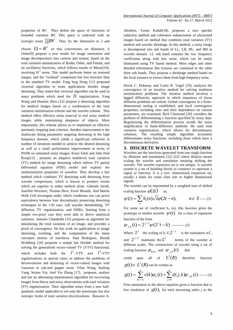
index k, and the scale parameter j. Figure (2 a) shows the
structure of two stages down sampling filter banks in terms of
coefficients.
(a) Two stages down sampling Filter bank
(b) Two stages up sampling filter.
Fig 2: down sampling and up sampling filter.
(a): Row wise decomposition (b) One dimensional decomposition (c)Two dimensional decomposition
Fig 3: Two-dimensional wavelet transform
A reconstruction of the original fine scale coefficient of the
signal made from a combination of the scaling function and
wavelet coefficient at a course resolution is derived by
considering a signal in the j+1 scaling function space
1)( jtf . Figure (2 b) shows the structure of two
stages up sampling filter banks in terms of coefficients i.e.
synthesis from coarse scale to fine scale [23] [24] [25].
The DWT is identical with a hierarchical sub band system
where the sub bands are logarithmically spaced in frequency
and represent octave-band decomposition. By applying DWT,
the image is actually divided i.e. decomposed into four sub
bands and critically sub-sampled as shown in Figure (3 a).
These four sub bands arise from separable applications of
vertical and horizontal analysis filters for wavelet
decomposition as shown in Figure (3 b). The filters h0 and h1
shown in Figure (2) are one-dimensional Low Pass Filter
(LPF) and High Pass Filter (HPF), respectively. Thus,
decomposition provides sub bands corresponding to different
resolution levels and orientation.
These sub bands labeled LH, LH, HL and HH represent the
finest scale wavelet coefficients, i.e. detail images while the
sub band LL corresponds to coarse level coefficients, i.e.
approximation image. To obtain the next coarse level of
wavelet coefficients, the sub band LL alone is further
decomposed and critically sampled using similar filter bank
shown in Figure (2). This results in two-level wavelet
decomposition as shown in Figure (3 c). The decomposed
image can be reconstructed using a reconstruction (i.e. Inverse
DWT) or synthesis filter.
4. PROPOSED VARIATION
TECHNIQUE Image denoising is one of the measure issues in image
processing, not only because it plays a key preliminary role in
many computer vision systems, but also because it is probably
the simplest way to address the fundamental issue of image
dj
g0(n)
g1(n)
g0(n)
2
2
2
2 g1(n)
cj-1
dj-1
cj+1
cj
2
2
2
h1(-n)
h0(-n)
dj
cj
dj+1
cj+1
h1(-n)
h0(-n)
cj+1
2
L H
LL
LH
HL
HH
LL
LH
LH
HH
LH
HL
HH
International Journal of Computer Applications (0975 – 8887)
Volume 42– No.17, March 2012
11
modeling, as a starting point towards more complex tasks like
deblurring, demosaicking, in painting, etc. We propose the
new method to determine variation around the neighbor and
modify the pixel according to the energy in that block. A
discretized gradient for an image NRf is defined as
),(),,((),( jifjifjif yx where
otherwise 0
1-ni0 if ),(),1(),(
jifjif
jifx
otherwise 0
1-nj0 if ),()1,(),(
jifjif
jify
These equations give the gradient with respect to horizontal
and vertical axis in image. Figure (4) shows a technique of
horizontal, vertical and neighboring variation proposed model
where, X is marked as the location of the pixel in an image.
(a)Horizontal Variation (b) Vertical Variation
(c) Cluster Variation
Fig 4: Variation Model
4.1 Horizontal Variation: We propose a wavelet based Variation denoising scheme. In
our scheme, the wavelet coefficients are selected and modified
by applying the horizontal and vertical variation model.
The horizontal variation model applied to the image noisy
image patch.
n
j
jiji XXH1
1,,var )(
Where, Hvar is the horizontal variation. To obtain the
regularization parameter of the patch we need to calculate
energy of the patch.
nm
ji
jiX,
,
,nm1Energy
varH
Energy
Where, is the regularization parameter of the patch. The
coefficient can be modified by
nm
ji
X
ji
jiX,
,
,
,
The horizontal coefficients are get modified by regularization
parameter.
A. Vertical Variation
The vertical variation model applied to the image noisy image
patch.
n
i
jiji XXV1
,1,var )(
here, Hvar is the horizontal variation. To obtain the
regularization parameter of the patch we need to calculate
energy of the patch.
nm
ji
jinmXEnergy
,
,
,1
varV
Energy
Where, is the regularization parameter of the patch. The
coefficient can be modified by
nm
ji
X
ji
jiX,
,
,
,
The vertical coefficients are get modified by regularization
parameter.
4.2 Cluster Variation The cluster variation can be obtained by measuring the
variation at its neighbor. Consider 3*3 clusters apply to the
wavelet as shown in figure (5).
1,1,11,1
1,,1,
1,1,11,1
jijiji
jijiji
jijiji
Fig 5: 3*3 cluster
d (1) =(x (i, j)-x (i-1,j-1))
d(2) =(x(i,j)-x(i-1,j))
d(3) =(x(i,j)-x(i-1,j+1))
d(4) =(x(i,j)-x(i,j-1))
d(5) =(x(i,j)-x(i,j+1))
d(6) =(x(i,j)-x(i+1,j-1))
d(7) =(x(i,j)-x(i+1,j))
d(8) =(x(i,j)-x(i+1,j+1))
8
1
1
k
kkdd
The obtained cluster variation coefficients d will be replaced
by modified coefficients x (i, j). Repeat this procedure to all
sub band of Wavelet Transform and modified the Wavelet
coefficient. This 3*3 mask will move through the sub band
International Journal of Computer Applications (0975 – 8887)
Volume 42– No.17, March 2012
12
and get modified coefficients. This method will not add any
blur in the image.
5. IMPLEMENTATION AND RESULTS We demonstrate the Variation scheme for removing
noise. The wavelet Variation scheme allows us to modify the
wavelet coefficients primarily in the high frequency domain.
The proposed variation model obtained through the horizontal
and vertical variation technique gives comparative result at all
type of noise. The coefficients modified at any level patch by
patch in this technique. The horizontal and vertical variation
technique gives us the threshold value at each level of the sub
band. These threshold coefficients will further modified by
taking inverse Wavelet Transform. The noise is removed by
taking the inverse wavelet transform of modified coefficients.
The cluster variation is performed by modification of each
pixel done at the center pixel level at all direction. This 3*3
mask will be moving in the each sub band of decomposed
Wavelet. This modified Wavelet coefficients at each
decomposition level using cluster variation will further
processed. This sub band will further up sampled by inverse
Wavelet Transform. We get better result to all types of noise
for this variation based regularization method with wavelet as
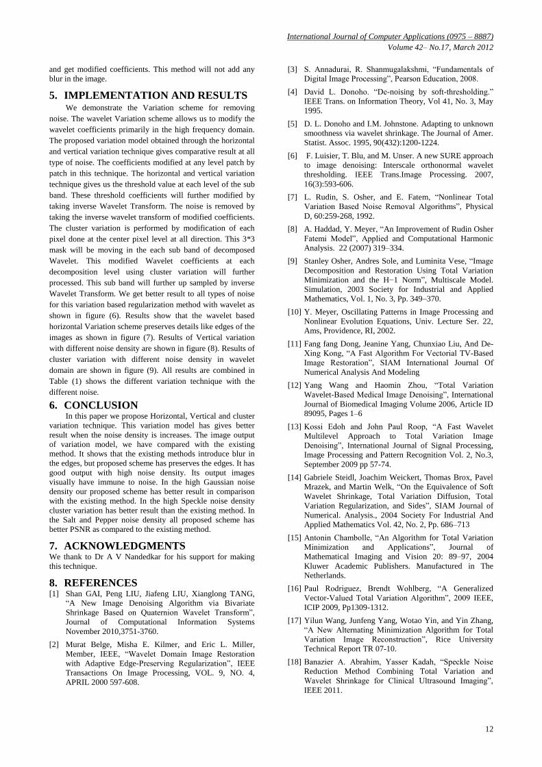
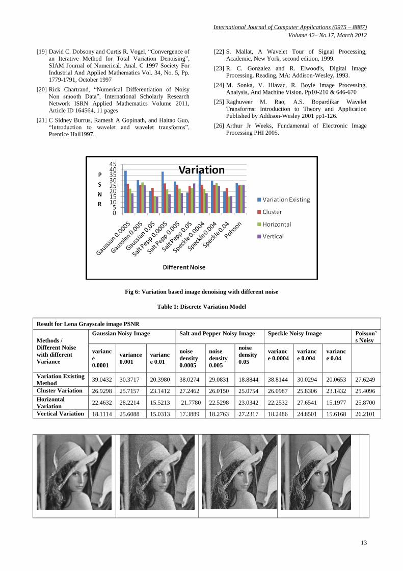
shown in figure (6). Results show that the wavelet based
horizontal Variation scheme preserves details like edges of the
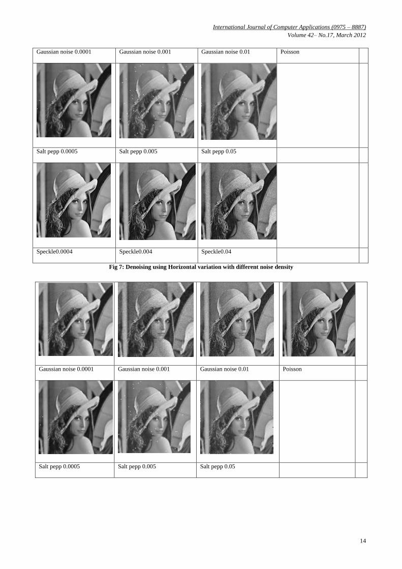
images as shown in figure (7). Results of Vertical variation
with different noise density are shown in figure (8). Results of
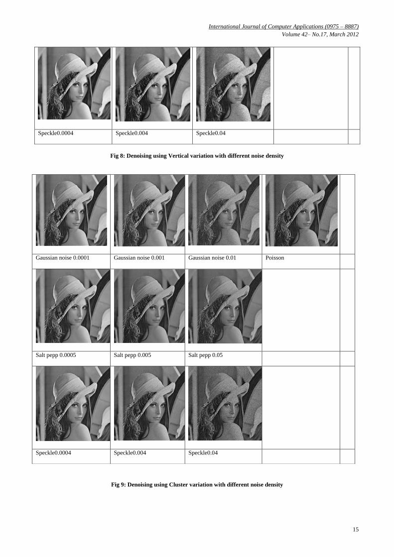
cluster variation with different noise density in wavelet
domain are shown in figure (9). All results are combined in
Table (1) shows the different variation technique with the
different noise.
6. CONCLUSION In this paper we propose Horizontal, Vertical and cluster
variation technique. This variation model has gives better
result when the noise density is increases. The image output
of variation model, we have compared with the existing
method. It shows that the existing methods introduce blur in
the edges, but proposed scheme has preserves the edges. It has
good output with high noise density. Its output images
visually have immune to noise. In the high Gaussian noise
density our proposed scheme has better result in comparison
with the existing method. In the high Speckle noise density
cluster variation has better result than the existing method. In
the Salt and Pepper noise density all proposed scheme has
better PSNR as compared to the existing method.
7. ACKNOWLEDGMENTS We thank to Dr A V Nandedkar for his support for making
this technique.
8. REFERENCES [1] Shan GAI, Peng LIU, Jiafeng LIU, Xianglong TANG,
“A New Image Denoising Algorithm via Bivariate
Shrinkage Based on Quaternion Wavelet Transform”,
Journal of Computational Information Systems
November 2010,3751-3760.
[2] Murat Belge, Misha E. Kilmer, and Eric L. Miller,
Member, IEEE, “Wavelet Domain Image Restoration
with Adaptive Edge-Preserving Regularization”, IEEE
Transactions On Image Processing, VOL. 9, NO. 4,
APRIL 2000 597-608.
[3] S. Annadurai, R. Shanmugalakshmi, “Fundamentals of
Digital Image Processing”, Pearson Education, 2008.
[4] David L. Donoho. “De-noising by soft-thresholding.”
IEEE Trans. on Information Theory, Vol 41, No. 3, May
1995.
[5] D. L. Donoho and I.M. Johnstone. Adapting to unknown
smoothness via wavelet shrinkage. The Journal of Amer.
Statist. Assoc. 1995, 90(432):1200-1224.
[6] F. Luisier, T. Blu, and M. Unser. A new SURE approach
to image denoising: Interscale orthonormal wavelet
thresholding. IEEE Trans.Image Processing. 2007,
16(3):593-606.
[7] L. Rudin, S. Osher, and E. Fatem, “Nonlinear Total
Variation Based Noise Removal Algorithms”, Physical
D, 60:259-268, 1992.
[8] A. Haddad, Y. Meyer, “An Improvement of Rudin Osher
Fatemi Model”, Applied and Computational Harmonic
Analysis. 22 (2007) 319–334.
[9] Stanley Osher, Andres Sole, and Luminita Vese, “Image
Decomposition and Restoration Using Total Variation
Minimization and the H−1 Norm”, Multiscale Model.
Simulation, 2003 Society for Industrial and Applied
Mathematics, Vol. 1, No. 3, Pp. 349–370.
[10] Y. Meyer, Oscillating Patterns in Image Processing and
Nonlinear Evolution Equations, Univ. Lecture Ser. 22,
Ams, Providence, RI, 2002.
[11] Fang fang Dong, Jeanine Yang, Chunxiao Liu, And De-
Xing Kong, “A Fast Algorithm For Vectorial TV-Based
Image Restoration”, SIAM International Journal Of
Numerical Analysis And Modeling
[12] Yang Wang and Haomin Zhou, “Total Variation
Wavelet-Based Medical Image Denoising”, International
Journal of Biomedical Imaging Volume 2006, Article ID
89095, Pages 1–6
[13] Kossi Edoh and John Paul Roop, “A Fast Wavelet
Multilevel Approach to Total Variation Image
Denoising”, International Journal of Signal Processing,
Image Processing and Pattern Recognition Vol. 2, No.3,
September 2009 pp 57-74.
[14] Gabriele Steidl, Joachim Weickert, Thomas Brox, Pavel
Mrazek, and Martin Welk, “On the Equivalence of Soft
Wavelet Shrinkage, Total Variation Diffusion, Total
Variation Regularization, and Sides”, SIAM Journal of
Numerical. Analysis., 2004 Society For Industrial And
Applied Mathematics Vol. 42, No. 2, Pp. 686–713
[15] Antonin Chambolle, “An Algorithm for Total Variation
Minimization and Applications”, Journal of
Mathematical Imaging and Vision 20: 89–97, 2004
Kluwer Academic Publishers. Manufactured in The
Netherlands.
[16] Paul Rodriguez, Brendt Wohlberg, “A Generalized
Vector-Valued Total Variation Algorithm”, 2009 IEEE,
ICIP 2009, Pp1309-1312.
[17] Yilun Wang, Junfeng Yang, Wotao Yin, and Yin Zhang,
“A New Alternating Minimization Algorithm for Total
Variation Image Reconstruction”, Rice University
Technical Report TR 07-10.
[18] Banazier A. Abrahim, Yasser Kadah, “Speckle Noise
Reduction Method Combining Total Variation and
Wavelet Shrinkage for Clinical Ultrasound Imaging”,
IEEE 2011.
International Journal of Computer Applications (0975 – 8887)
Volume 42– No.17, March 2012
13
[19] David C. Dobsony and Curtis R. Vogel, “Convergence of
an Iterative Method for Total Variation Denoising”,
SIAM Journal of Numerical. Anal. C 1997 Society For
Industrial And Applied Mathematics Vol. 34, No. 5, Pp.
1779-1791, October 1997
[20] Rick Chartrand, “Numerical Differentiation of Noisy
Non smooth Data”, International Scholarly Research
Network ISRN Applied Mathematics Volume 2011,
Article ID 164564, 11 pages
[21] C Sidney Burrus, Ramesh A Gopinath, and Haitao Guo,
“Introduction to wavelet and wavelet transforms”,
Prentice Hall1997.
[22] S. Mallat, A Wavelet Tour of Signal Processing,
Academic, New York, second edition, 1999.
[23] R. C. Gonzalez and R. Elwood's, Digital Image
Processing. Reading, MA: Addison-Wesley, 1993.
[24] M. Sonka, V. Hlavac, R. Boyle Image Processing,
Analysis, And Machine Vision. Pp10-210 & 646-670
[25] Raghuveer M. Rao, A.S. Bopardikar Wavelet
Transforms: Introduction to Theory and Application
Published by Addison-Wesley 2001 pp1-126.
[26] Arthur Jr Weeks, Fundamental of Electronic Image
Processing PHI 2005.
Fig 6: Variation based image denoising with different noise
Table 1: Discrete Variation Model
Result for Lena Grayscale image PSNR
Methods /
Different Noise
with different
Variance
Gaussian Noisy Image Salt and Pepper Noisy Image Speckle Noisy Image Poisson’
s Noisy
varianc
e
0.0001
variance
0.001
varianc
e 0.01
noise
density
0.0005
noise
density
0.005
noise
density
0.05
varianc
e 0.0004
varianc
e 0.004
varianc
e 0.04
Variation Existing
Method 39.0432 30.3717 20.3980 38.0274 29.0831 18.8844 38.8144 30.0294 20.0653 27.6249
Cluster Variation 26.9298 25.7157 23.1412 27.2462 26.0150 25.0754 26.0987 25.8306 23.1432 25.4096
Horizontal
Variation 22.4632 28.2214 15.5213 21.7780 22.5298 23.0342 22.2532 27.6541 15.1977 25.8700
Vertical Variation 18.1114 25.6088 15.0313 17.3889 18.2763 27.2317 18.2486 24.8501 15.6168 26.2101
International Journal of Computer Applications (0975 – 8887)
Volume 42– No.17, March 2012
14
Gaussian noise 0.0001 Gaussian noise 0.001 Gaussian noise 0.01 Poisson
Salt pepp 0.0005 Salt pepp 0.005 Salt pepp 0.05
Speckle0.0004 Speckle0.004 Speckle0.04
Fig 7: Denoising using Horizontal variation with different noise density
Gaussian noise 0.0001 Gaussian noise 0.001 Gaussian noise 0.01 Poisson
Salt pepp 0.0005 Salt pepp 0.005 Salt pepp 0.05
International Journal of Computer Applications (0975 – 8887)
Volume 42– No.17, March 2012
15
Fig 8: Denoising using Vertical variation with different noise density
Fig 9: Denoising using Cluster variation with different noise density
Speckle0.0004 Speckle0.004 Speckle0.04
Gaussian noise 0.0001 Gaussian noise 0.001 Gaussian noise 0.01 Poisson
Salt pepp 0.0005 Salt pepp 0.005 Salt pepp 0.05
Speckle0.0004 Speckle0.004 Speckle0.04

![Optimal rates for total variation denoising - arXiv · arXiv:1603.09388v3 [math.ST] 16 Jun 2016 Optimal rates for total variation denoising Jan-Christian H¨utter and Philippe Rigollet](https://img.pdfslide.net/doc/110x75/5b84535b7f8b9a784a8c10c1/optimal-rates-for-total-variation-denoising-arxiv-arxiv160309388v3-mathst.jpg)


![Analogue of the Total Variation Denoising Model in the ...esedoglu/Papers_Preprints/elsey_esedoglu.pdftotal variation based image denoising model of Rudin, Osher, and Fatemi [32] (ROF)](https://img.pdfslide.net/doc/110x75/5f09a4607e708231d427d056/analogue-of-the-total-variation-denoising-model-in-the-esedoglupaperspreprintselsey.jpg)