Embed Size (px)
Citation preview

Digital Image Processing
Image Enhancement in the
Frequency Domain
(Chapter 5)

Any function that periodically repeats itself can be expressedas the sum of sines and/or cosines of different frequencies, each multiplied by a different coefficients.This sum is called a Fourierseries.
Fourier Series

00
0
00
0
00
0
0
0
0
0
0
0
1
000
sin)(2
cos)(2
)(1
sincos)(
Tt
t
n
Tt
t
n
Tt
t
n
nn
dttnwtgT
b
dttnwtgT
a
dttgT
a
tnwbtnwaatg
Fourier Series

A function that is not periodic but the area under its curve is finite can be expressed as the integral of sines and/or cosines multiplied by a weighing function. The formulation in this case is Fourier transform.
Fourier Transform
dueuFxf
dxexfuF
uxj
uxj
2
2
)()(
)()(
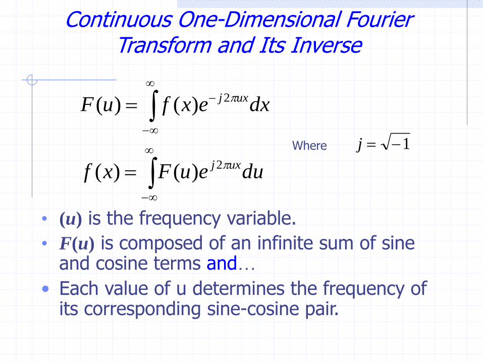
Continuous One-Dimensional Fourier Transform and Its Inverse
Where 1j
• (u) is the frequency variable.
• F(u) is composed of an infinite sum of sine and cosine terms and…
• Each value of u determines the frequency of its corresponding sine-cosine pair.

2
10
2
11
)(
x
xx
2 sinc )(
uuF
0.5- 0.5
x
2
4
u
Continuous One-Dimensional Fourier Transform and Its Inverse
ExampleFind the Fourier transform of a gate function (t) defined by

Discrete One-Dimensional Fourier Transform and Its Inverse
• A continuous function f(x) is discretized into a sequence:
)}]1[(),...,2(),(),({ 0000 xNxfxxfxxfxf
by taking N or M samples x units apart.

Discrete One-Dimensional Fourier Transform and Its Inverse
• Where x assumes the discrete values (0,1,2,3,…,M-1) then
)()( 0 xxxfxf
• The sequence {f(0),f(1),f(2),…f(M-1)} denotes any
M uniformly spaced samples from a corresponding
continuous function.

1
0
1
0
2
2sin2cos)(1
)(
)(1
)(
M
x
M
x
M
xuj
M
xuj
M
xuxf
MuF
exfM
uF
1
0
2
)()(M
u
xM
uj
euFxf
u =[0,1,2, …, M-1]
x =[0,1,2, …, M-1]
Discrete One-Dimensional Fourier Transform and Its Inverse

Discrete One-Dimensional Fourier Transform and Its Inverse
• The values u = 0, 1, 2, …, M-1 correspond to
samples of the continuous transform at values 0, u, 2u, …, (M-1)u.
i.e. F(u) represents F(uu), where:
u 1
Mx

Discrete One-Dimensional Fourier Transform and Its Inverse
• The Fourier transform of a real function is generally complex and we use polar coordinates:
• Its phase angle
)(
)(tan)(
)]()([)(
)()(
)()()(
1
2/122
)(
uR
uIu
uIuRuF
euFuF
ujIuRuF
uj

• The square of the spectrum
)()()()( 222uIuRuFuP
is referred to as the Power Spectrum of f(x)
(spectral density).
Discrete One-Dimensional Fourier Transform and Its Inverse

• Fourier spectrum: 2/122 ),(),(),( vuIvuRvuF
• Phase:
),(
),(tan),( 1
vuR
vuIvu
• Power spectrum: ),(),(),(),( 222vuIvuRvuFvuP
Discrete 2-Dimensional Fourier Transform

Discrete One-Dimensional Fourier Transform and Its Inverse
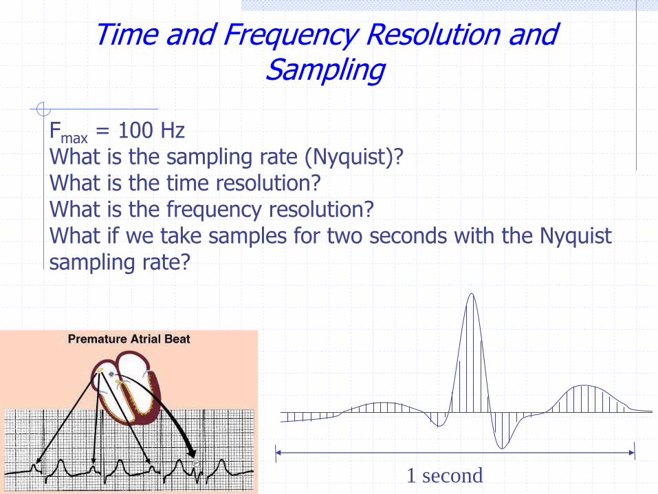
1 second
Fmax = 100 HzWhat is the sampling rate (Nyquist)?What is the time resolution?What is the frequency resolution?What if we take samples for two seconds with the Nyquist sampling rate?
Time and Frequency Resolution and Sampling

2/122
1
0
1
0
)(2
1
0
1
0
)(2
),(),(),(
),(),(
),(1
),(
vuIvuRvuF
evuFyxf
eyxfMN
vuF
M
u
N
v
yN
vx
M
uj
M
x
N
y
N
yv
M
xuj
Fourier Spectrum
Discrete Two-Dimensional Fourier Transform and Its Inverse
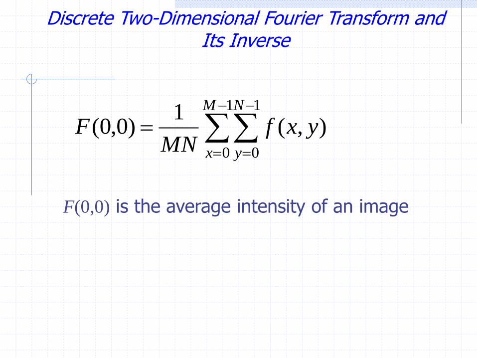
1
0
1
0
),(1
)0,0(M
x
N
y
yxfMN
F
F(0,0) is the average intensity of an image
Discrete Two-Dimensional Fourier Transform and Its Inverse

Use Matlab to generate the above figures
Discrete Two-Dimensional Fourier Transform and Its Inverse

),(),(
)()(
then
)()(
If
00
)(2
0
00
0
vvuuFeyxf
Getg
Gtg
N
yv
M
xuj
tj
Frequency Shifting Property of the Fourier Transform

Frequency Shifting Property of the Fourier Transform

function Normalized_DFT = Img_DFT(img)
img=double(img); % So mathematical operations can be conducted on
% the image pixels.
[R,C]=size(img);
for r = 1:R % To phase shift the image so the DFT will be
for c=1:C % centered on the display monitor
phased_img(r,c)=(img(r,c))*(-1)^(r+c);
end
end
fourier_img = fft2(phased_img); %Discrete Fourier Transform
mag_fourier_img = abs(fourier_img ); % Magnitude of DFT
Log_mag_fourier_img = log10(mag_fourier_img +1);
Max = max(max(Log_mag_fourier_img ));
Normalized_DFT = (Log_ mag_fourier_img )*(255/Max);
imshow(uint8(Normalized_DFT))
Basic Filtering in the Frequency Domain using Matlab

1. Multiply the input image by (-1)x+y to center the transform2. Compute F(u,v), the DFT of the image from (1)3. Multiply F(u,v) by a filter function H(u,v)4. Compute the inverse DFT of the result in (3)5. Obtain the real part of the result in (4)6. Multiply the result in (5) by (-1)x+y
Basic Filtering in the Frequency Domain

An image and its Frequency information
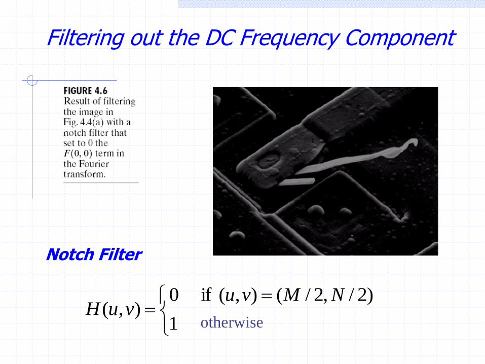
1
)2/,2/(),( if 0),(
NMvuvuH
otherwise
Notch Filter
Filtering out the DC Frequency Component

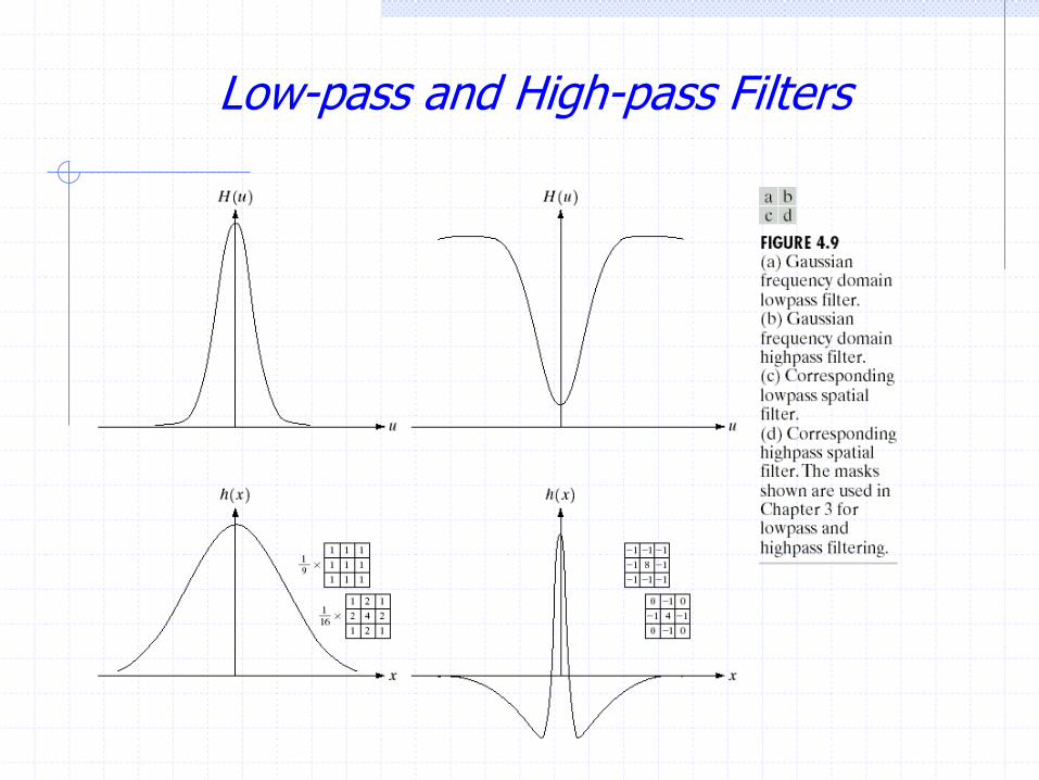
Low Pass Filter attenuate high frequencies while “passing” low frequencies.
High Pass Filterattenuate low frequencies while “passing” high frequencies.
Low-pass and High-pass Filters

High-pass Filtering
Low-pass and High-pass Filters
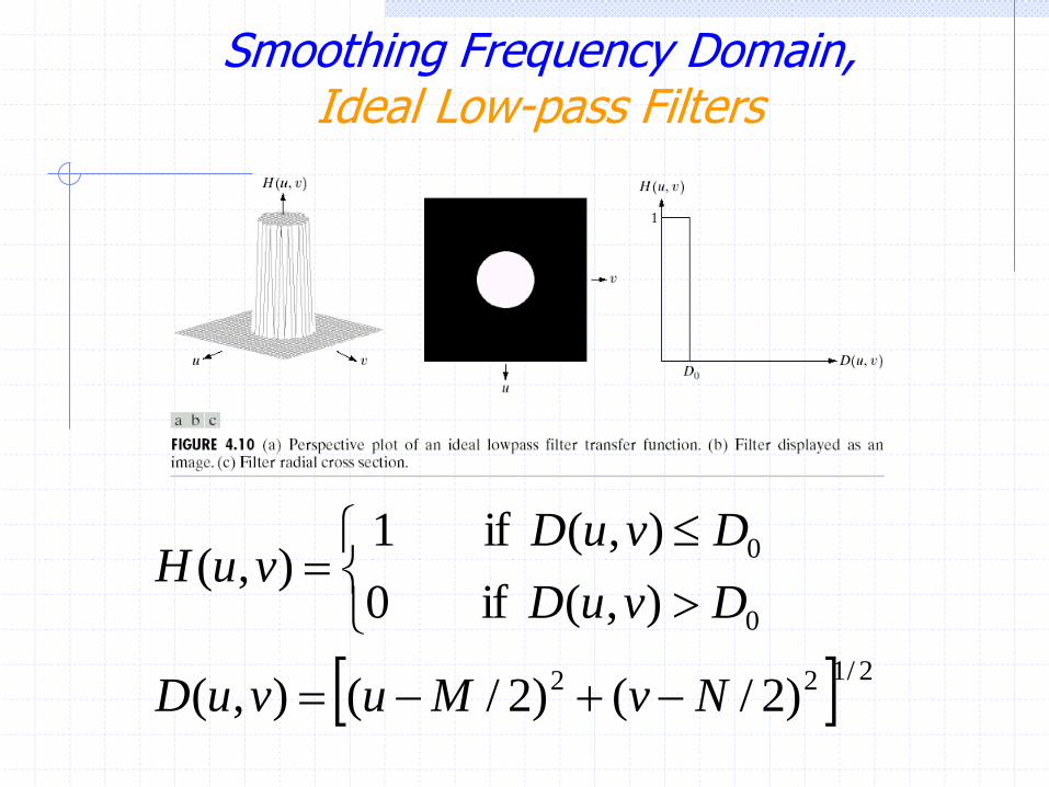
2/122
0
0
)2/()2/(),(
),( if 0
),( if 1),(
NvMuvuD
DvuD
DvuDvuH
Smoothing Frequency Domain, Ideal Low-pass Filters
u v
T
M
u
N
v
T
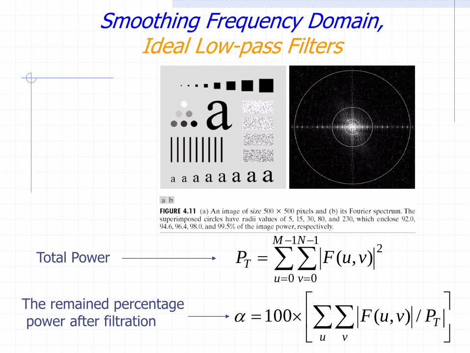
PvuF
vuFP
/),(100
),(1
0
1
0
2
Total Power
The remained percentagepower after filtration
Smoothing Frequency Domain, Ideal Low-pass Filters

For circle radius fc =5
Enclose image power = 92%
fc =15
= 94.6%
fc =30
= 96.4%
fc =80
= 98%fc =230
= 99.5%
Smoothing Frequency Domain,Ideal Low-pass Filters

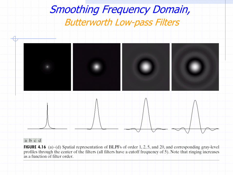
Cause of Ringing

nDvuD
vuH2
0/),(1
1),(
Smoothing Frequency Domain, Butterworth Low-pass Filters

Smoothing Frequency Domain, Butterworth Low-pass Filters
Radii= 5
Radii= 15Radii= 30
Radii= 80 Radii= 230
Butterworth Low-pass Filter: n=2
Smoothing Frequency Domain,Butterworth Low-pass Filters

20
2 2/),(),(
DvuDevuH
Smoothing Frequency Domain, Gaussian Low-pass Filters

Radii= 5
Radii= 15Radii= 30
Radii= 80 Radii= 230
Gaussian Low-pass
Smoothing Frequency Domain, Gaussian Low-pass Filters

Smoothing Frequency Domain, Gaussian Low-pass Filters

Smoothing Frequency Domain, Gaussian Low-pass Filters

Smoothing Frequency Domain, Gaussian Low-pass Filters

Hhp(u,v) = 1 - Hlp(u,v)
Ideal HPF
Butterworth HPF
Gaussian HPF
Sharpening Frequency Domain Filters

Sharpening Frequency Domain Filters

),( if 1
),( if 0),(
0
0
DvuD
DvuDvuH
Sharpening Frequency Domain, Ideal High-pass Filters

nvuDD
vuH2
0 ),(/1
1),(
Sharpening Frequency Domain,Butterworth High-pass Filters

20
2 2/),(1),(
DvuDevuH
Sharpening Frequency Domain,Gaussian High-pass Filters

Homomorphic Filtering

Homomorphic Filtering

g t k t h tM
k t m h mm
M
( ) ( ) * ( ) ( ) ( )
1
0
1
h(t) g(t)k(t)g(t) = k(t)*h(t)
G(f) = K(f)H(f)
-1
1
t
h(t)
1
2
3
t
k(t)
1 2 3
* is a convolution operator and not multiplication
Convolution
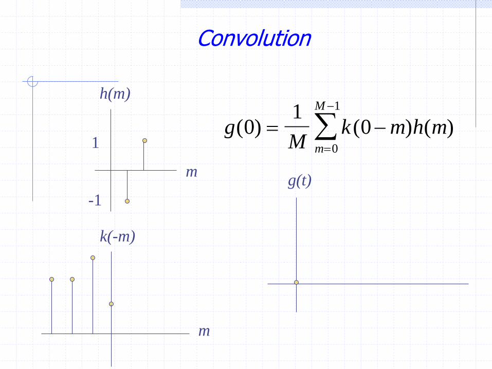
gM
k m h mm
M
( ) ( ) ( )01
00
1
m
k(-m)
-1
1
m
h(m)
g(t)
Convolution

-1
1
m
h(m)
Convolution
m
k(1-m)
g(t)

-1
1
m
h(m)
Convolution
m
k(2-m)
g(t)

-1
1
m
h(m)
Convolution
m
k(3-m)
g(t)

-1
1
m
h(m)
Convolution
m
k(4-m)
g(t)

-1
1
m
h(m)
Convolution
m
k(5-m)
g(t)

-1
1
m
h(m)
Convolution
m
k(6-m)
g(t)

f x y h x yMN
f m n h x m y nn
N
m
M
( , ) ( , ) ( , ) ( , )
1
0
1
0
1
2-Dimensions Convolution

g t k t h tM
k t m h mm
M
( ) ( ) ( ) ( ) ( )
1
0
1
h(t) g(t)k(t)g(t) = k(t)h(t)
G(f) = K(f)* H(f)
-1
1 1
2
t t
k(t)
h(t)
g(t)
2
Correlation

Correlation

Convolution

Convolution

Convolution

Convolution