Image Matching via Saliency Region Correspondences Alexander Toshev Jianbo Shi Kostas Daniilidis IEEE Conference on Computer Vision and Pattern Recognition

Image Matching via Saliency Region Correspondences

Alexander ToshevJianbo ShiKostas Daniilidis

IEEE Conference on Computer Vision and Pattern Recognition (CVPR), 2007

Outline

IntroductionJoint-Image Graph (JIG) Matching ModelOptimization in the JIGEstimation of Dense CorrespondencesImplementation DetailsExperimentsConclusion

Outline

IntroductionJoint-Image Graph (JIG) Matching ModelOptimization in the JIGEstimation of Dense Correspondences Implementation DetailsExperimentsConclusion

Introduction

Correspondence estimation is one of the fundamental challenges in computer vision lying in the core of many problems

To find the correspondence of interest points, whose power is in the ability to robustly capture discriminative image structures

Introduction

Feature-based approaches suffer from the ambiguity of local feature descriptors

To address matching ambiguities is to provide grouping constraints via segmentation

Disadvantage： changing drastically even for small deformation of the scene

Introduction

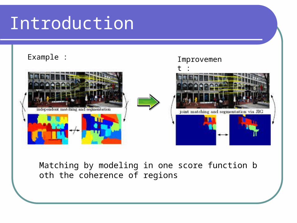
Example : Improvement :

Matching by modeling in one score function both the coherence of regions

Introduction

A pair of corresponding regions as co-salient define them as follows: Each region in the pair should exhibit strong

internal coherence with respect to the background in the image

The correspondence between the regions from the two images should be supported by high similarity of features extracted from these regions

Outline


Joint-Image Graph Matching Model

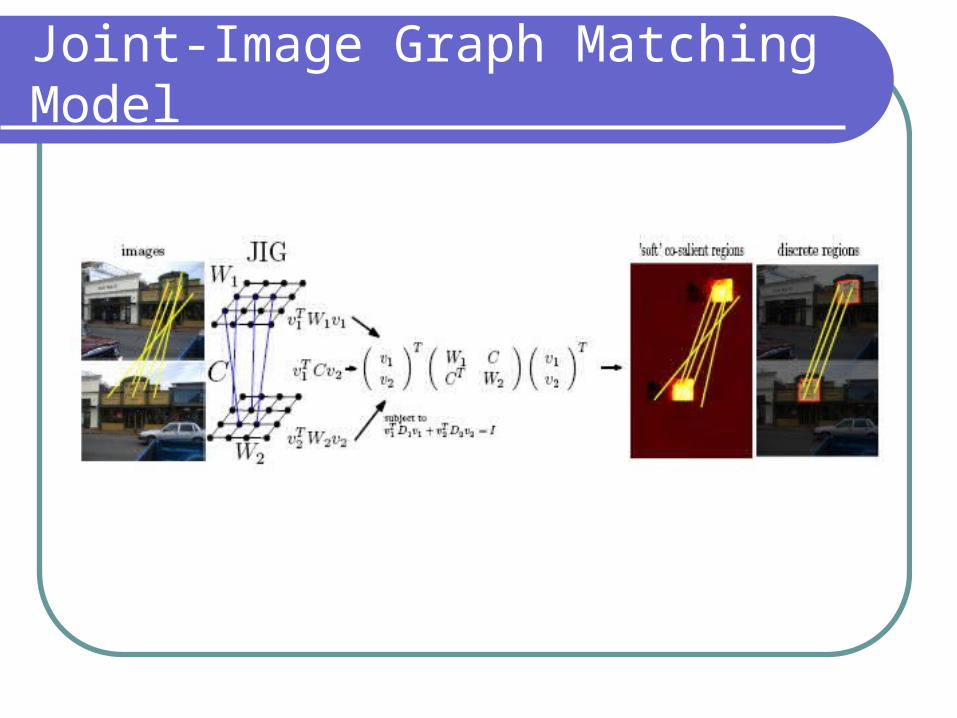
To formalize this model Introduce the joint-image graph (JIG) which contains vertices the pixels of both images edges represent intra-image similarities and inter-image

feature matches

A good cluster in the JIG consists of a pair of coherent segments describing corresponding scene parts from the two image


1 2

1

2

, ,

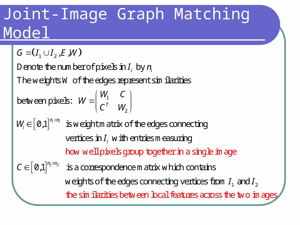
Denote the number of pixels in by

The weights W of the edges represent similarities

between pixels:

0,1 is weight matrix of the edges connecting

i i

i i

T

n n

i

G I I E W

I n

W CW

C W

W

1 2

how well pixels group together in a single imag

vertices in with entries measuring

0,1 is a correspondence matrix which contains

weigh

e

t

i

n n

I

C

1 2s of the edges connecting vertices from and

the similarities between local features across the two images

I I


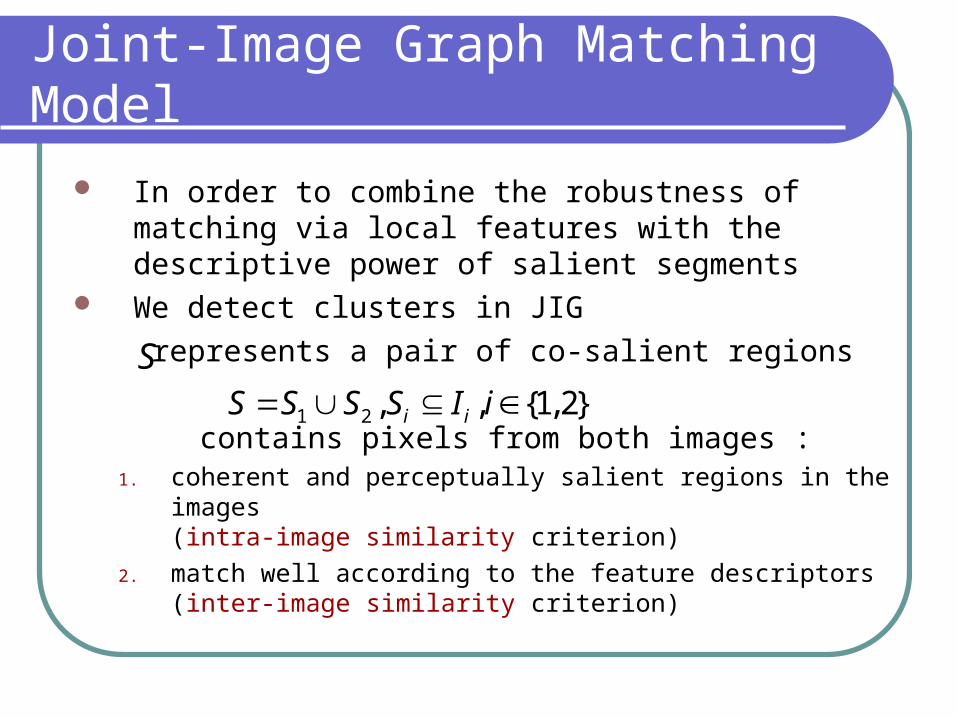
In order to combine the robustness of matching via local features with the descriptive power of salient segments

We detect clusters in JIG

represents a pair of co-salient regions

contains pixels from both images :1. coherent and perceptually salient regions in the images

(intra-image similarity criterion)

2. match well according to the feature descriptors (inter-image similarity criterion)

1 2 , , {1,2}i iS S S S I i S


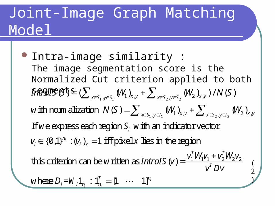
Intra-image similarity :The image segmentation score is the Normalized Cut criterion applied to both segments

1 1 2 2

1 1 2 2

1 , 2 ,, ,

1 , 2 ,, ,

( ) ( ( ) ( ) ) / ( )

with normalization ( ) ( ) ( )

If we express each region with an indicator vector

{0,1} : ( ) 1 iff pixel liei

x y x yx S y S x S y S

x y x yx S y I x S y I

i

ni i x

IntraIS S W W N S

N S W W

S

v v x

1 1 1 2 2 2

s in the region

this criterion can be written as ( )

where =W1 : 1 [1 1] i

i i

T T

T

nTi i n n

v W v v W vIntraIS v

v Dv

D

(2)


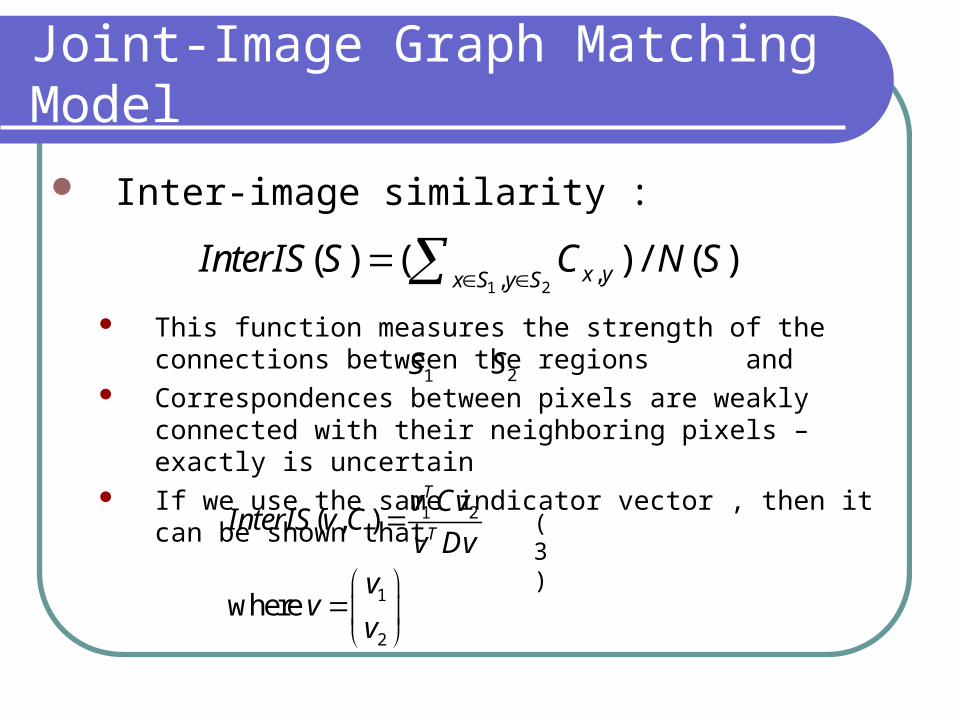
Inter-image similarity :

This function measures the strength of the connections

between the regions and Correspondences between pixels are weakly connected with

their neighboring pixels – exactly is uncertain If we use the same indicator vector , then it can be shown

that

1 2,,

( ) ( ) / ( )x yx S y SInterIS S C N S

1 2

1

2

( , )

where

T

T

v CvInterIS v C

v Dvv

vv

1S 2S

(3)


The correspondence matrix is defined in terms of feature correspondences encoded in a matrix

should select from pixel matches which connect each pixel of one of the images with at most one pixel of the other image

This can be written as

1 2n n

1/2 1/21 2

, , ,

( is the elementwise matrix multiplication)

with {0,1} , 1 ,and 1x y x y x yx y

D CD P M

P P P

MM

C

C


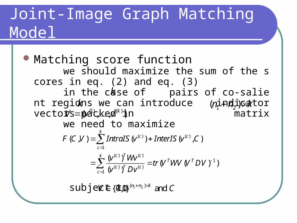
Matching score function we should maximize the sum of the scores in eq. (2) and eq. (3) in the case of pairs of co-salient regions we can introduce indicator vectors packed in matrix we need to maximize

subject to

kk 1 2( )n n k

(1) ( )( , , )kV v v

( ) ( )

1

( ) ( )1

( ) ( )1

( , ) ( ) ( , )

( )( ( ) )

( )

kc c

c

c T ckT T

c T cc

F C V IntraIS v InterIS v C

v Wvtr V WV V DV

v Dv

1 2( ){0,1} and n n kV C


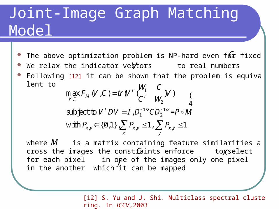
The above optimization problem is NP-hard even for fixed We relax the indicator vectors to real numbers Following [12] it can be shown that the problem is equivalent to

where is a matrix containing feature similarities across the images the constraints enforce to select for each pixel in one of the images only one pixel in the another which it can be mapped

1

,2

1/2 1/21 2

, , ,

max ( , ) ( ( ) )

subject to , =

with {0,1}, 1, 1

TM TV C

T

x y x y x yx y

W CF V C tr V V

C W

V DV I D CD P M

P P P

(4)

[12] S. Yu and J. Shi. Multiclass spectral clustering. In ICCV,2003

xy

C

V

MC


Outline

IntroductionJoint-Image Graph (JIG) Matching ModelOptimization in the JIGImplementation DetailsEstimation of Dense CorrespondencesExperimentsConclusion

Optimization in the JIG

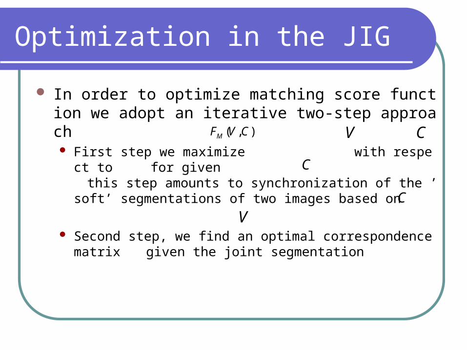
In order to optimize matching score function we adopt an iterative two-step approach First step we maximize with respect to for given

this step amounts to synchronization of the ’soft’ segmentations of two images based on

Second step, we find an optimal correspondence matrix given the joint segmentation

( , )MF V C CV

C

C

V


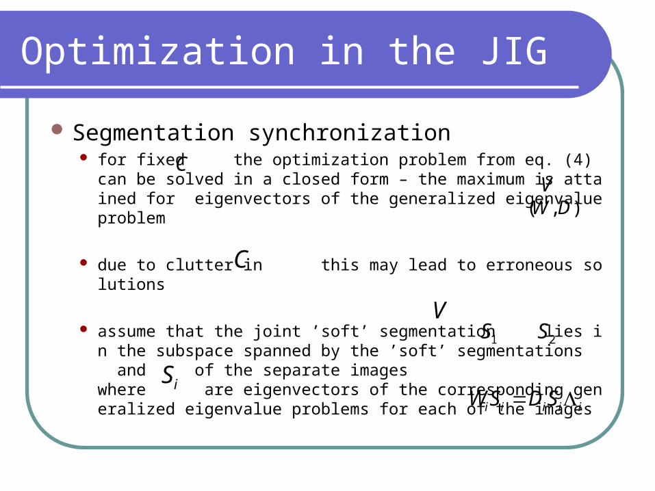
Segmentation synchronization for fixed the optimization problem from eq. (4) can be solve

d in a closed form – the maximum is attained for eigenvectors of the generalized eigenvalue problem

due to clutter in this may lead to erroneous solutions

assume that the joint ’soft’ segmentation lies in the subspace spanned by the ’soft’ segmentations and of the separate imageswhere are eigenvectors of the corresponding generalized eigenvalue problems for each of the images

1S 2S

iSi i i i iWS D S

C

V( , )W D

V

C


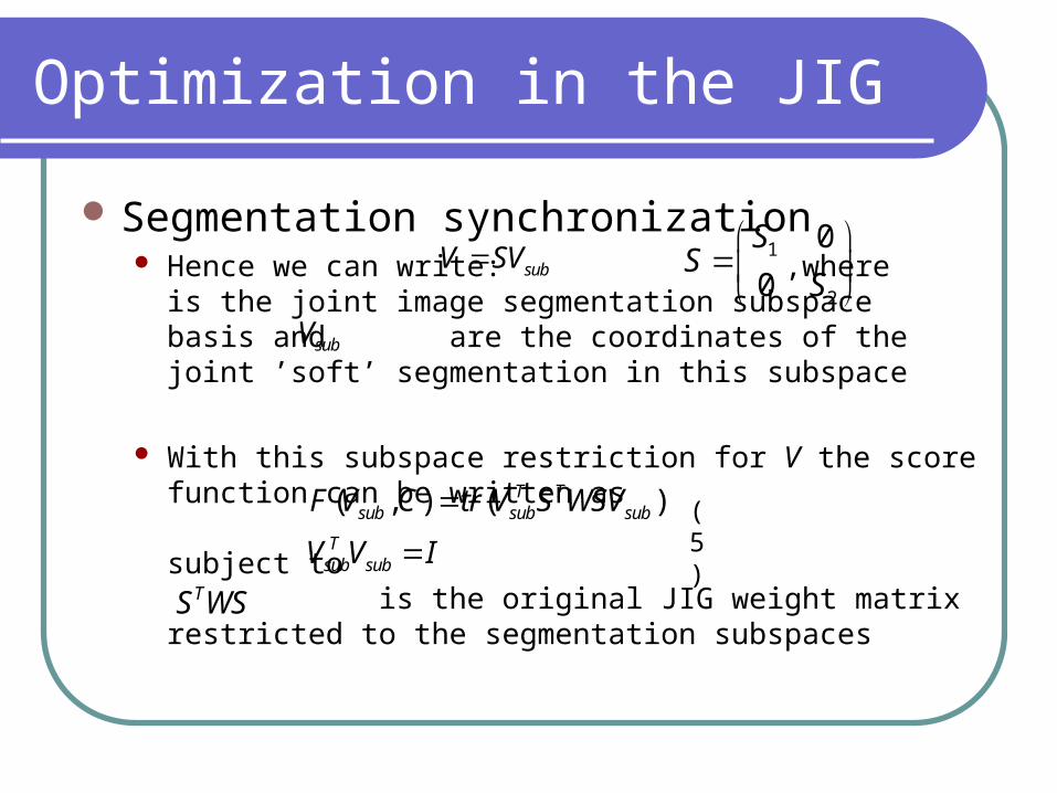
Segmentation synchronization Hence we can write: ,where

is the joint image segmentation subspace basis and are the coordinates of the joint ’soft’ segmentation in this subspace

With this subspace restriction for V the score function can be written as

subject to is the original JIG weight matrix restricted to the segmentation subspaces

subV SV 1

2

0

0

SS

S

subV

( , ) ( )T Tsub sub subF V C tr V S WSV (5

)Tsub subV V I

TS WS


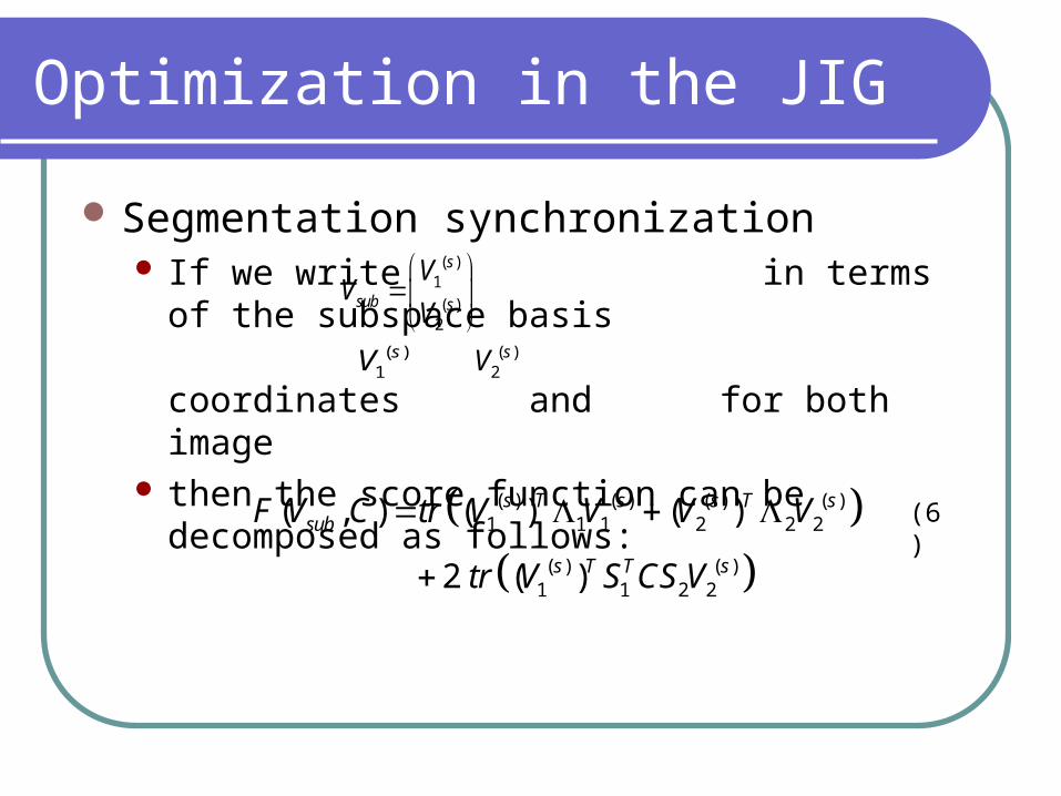
Segmentation synchronization If we write in terms of the subspace basis

coordinates and for both image then the score function can be decomposed as

follows:

( )1( )

2

s

sub s

VV

V

( )1sV ( )

2sV

( ) ( ) ( ) ( )1 1 1 2 2 2

( ) ( )1 1 2 2

( , ) ( ) ( )

2 ( )

s T s s T ssub

s T T s

F V C tr V V V V

tr V S CS V

(6)


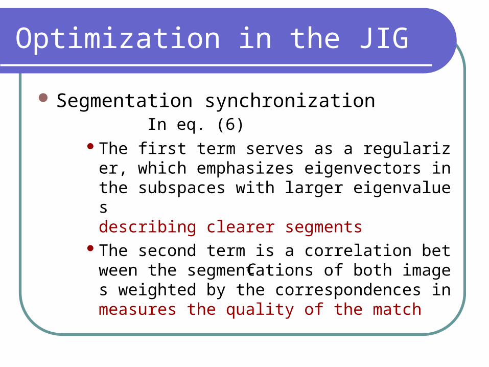
Segmentation synchronization In eq. (6)

The first term serves as a regularizer, which emphasizes eigenvectors in the subspaces with larger eigenvaluesdescribing clearer segments

The second term is a correlation between the segmentations of both images weighted by the correspondences inmeasures the quality of the match

C


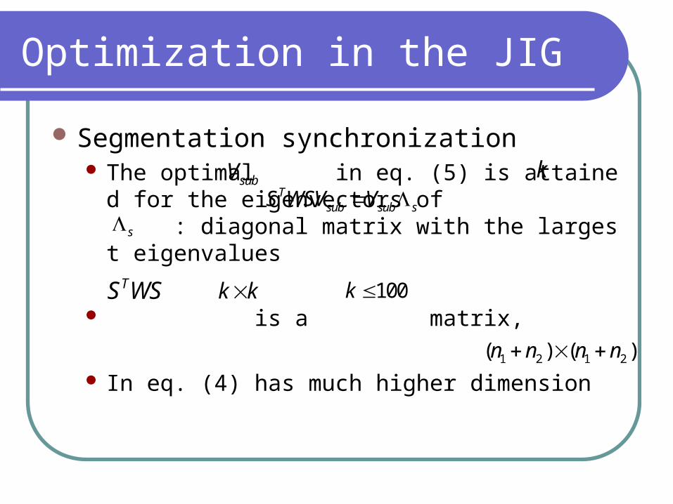
Segmentation synchronization The optimal in eq. (5) is attained for the eigenve

ctors of : diagonal matrix with the largest eigenvalues

is a matrix,

In eq. (4) has much higher dimension

subV kT

sub sub sS WSV V s

TS WS k k 100k

1 2 1 2( ) ( )n n n n


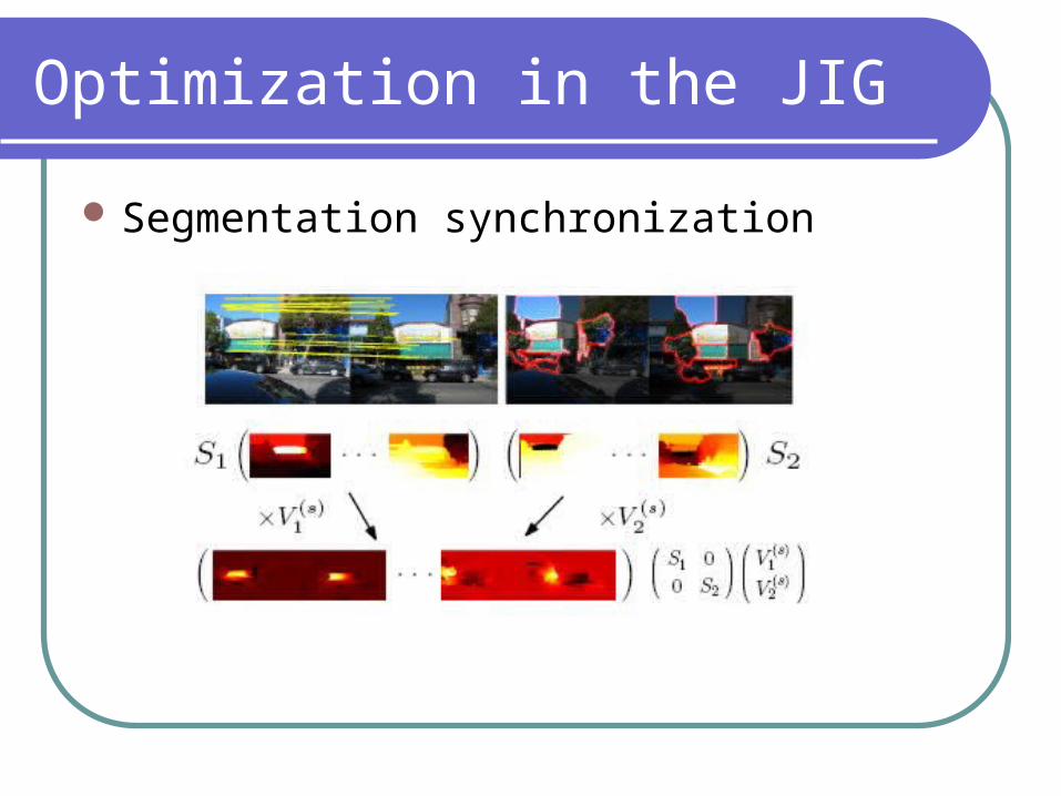
Segmentation synchronization


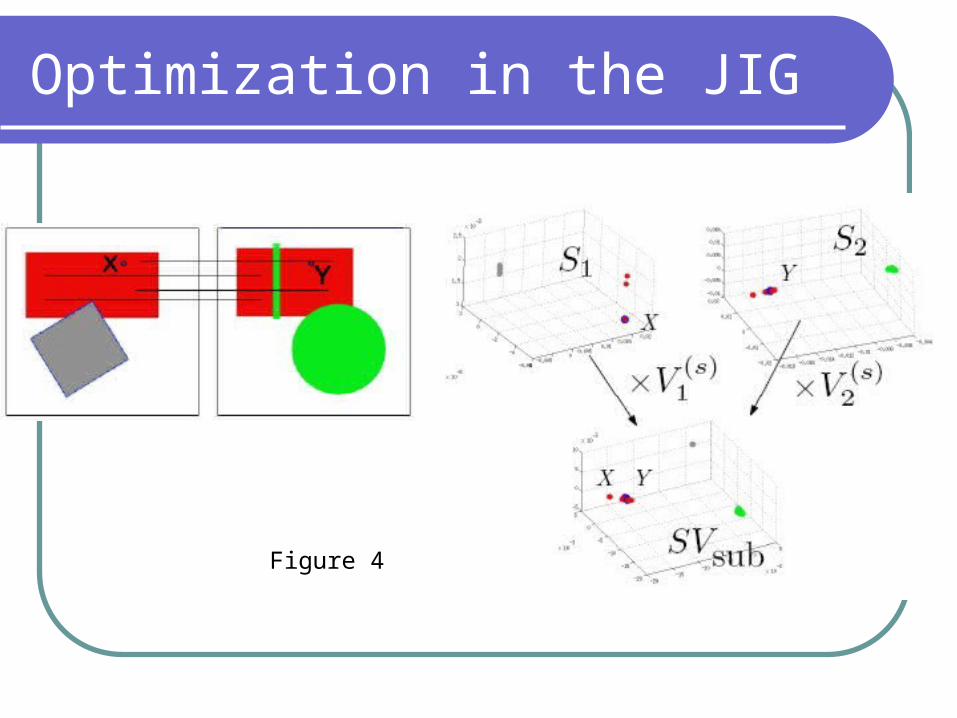
Segmentation synchronization A different view of the above process can be obtained by representing the eigenvectors by their rows: denote by the row of We can assign to each pixel in the image a k-dimensional vector which we will call the embedding vector of this pixel The segmentation synchronization can be viewed as a rotation of the segmentation embeddings of both images such that corresponding pixels are close in the embedding

sbths subSV

xbx


Figure 4


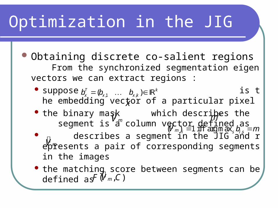
Obtaining discrete co-salient regions From the synchronized segmentation eigenvectors we can extract regions : suppose is the embedding vector

of a particular pixel the binary mask which describes the segment

is a column vector defined as describes a segment in the JIG and represents a

pair of corresponding segments in the images the matching score between segments can be define

d as

,1 ,( )T kx x x kb b b

xmV

thm

,( ) 1 iff arg maxm i s i sV b m

( , )mF V C

mV


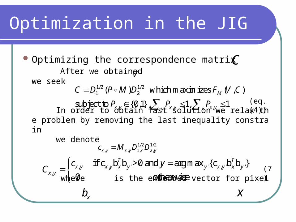
Optimizing the correspondence matrix After we obtained we seek

In order to obtain fast solution we relax the problem by removing the last inequality constrain we denote

where is the embedded vector for pixel

1/2 1/21 2

, , ,

( ) which maximizes ( , )

subject to {0,1}, 1, 1M

x y x y x yy x

C D P M D F V C

P P P

(eq. (4))

1/2 1/2, , 1, 2,x y x y x yc M D D

, , ' ' , ' ',

if c b b >0 and arg max {c b b }

0 otherwise

T Tx y x y x y y x y x y

x y

c yC

xb

(7)

x

V

C


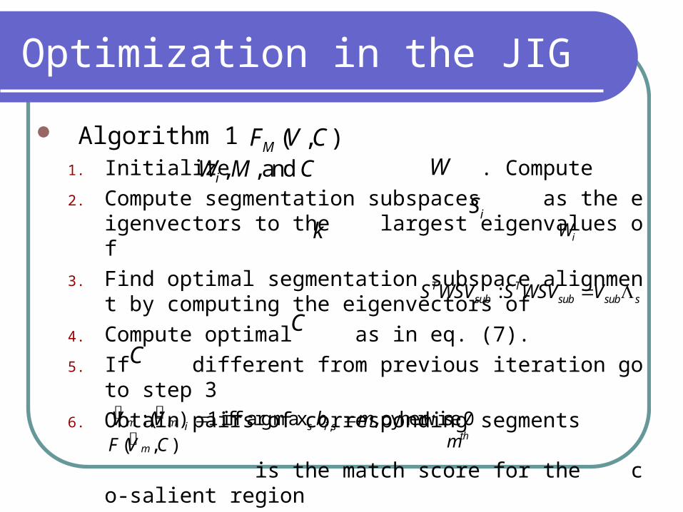
Algorithm 11. Initialize . Compute

2. Compute segmentation subspaces as the eigenvectors to the largest eigenvalues of

3. Find optimal segmentation subspace alignment by computing the eigenvectors of

4. Compute optimal as in eq. (7).

5. If different from previous iteration go to step 3

6. Obtain pairs of corresponding segments

is the match score for the co-salient region

( , )MF V C, , and iW M C W

iSiW

,: ( ) 1 iff arg max , oyherwise 0m m i s i sV V b m

( , )mF V Cthm

:T Tsub sub sub sS WSV S WSV V

C

C

k

Outline


Estimation of Dense Correspondences

Initially we choose a sparse set of feature matches extracted using a feature detector

In order to obtain denser set of correspondences we use a larger set of matches between features extracted everywhere in the image

Since this set can potentially contain many more wrong matches than , running algorithm 1 directly on does not give always satisfactory results

M

M

M

M


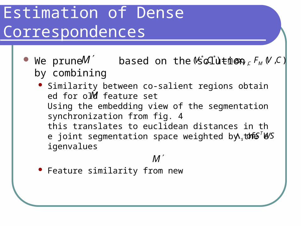
We prune based on the solution by combining Similarity between co-salient regions obtained for old featur

e set Using the embedding view of the segmentation synchronization from fig. 4this translates to euclidean distances in the joint segmentation space weighted by the eigenvalues

Feature similarity from new

M * *,( , ) max ( , )V C MV C F V C

of Ts S WS

M

M


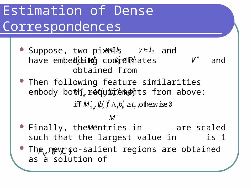
Suppose, two pixels and have embedding coordinates and obtained from

Then following feature similarities embody both requirements from above:

Finally, the entries in are scaled such that the largest value in is 1

The new co-salient regions are obtained as a solution of

1x I 2y I* kxb

* kyb

*V

* *, ,

* *,

( )

iff ( ) ,otherwise 0

Tx y x y x s y

Tx y x s y c

M M b b

M b b t

M M

( , )MF V C


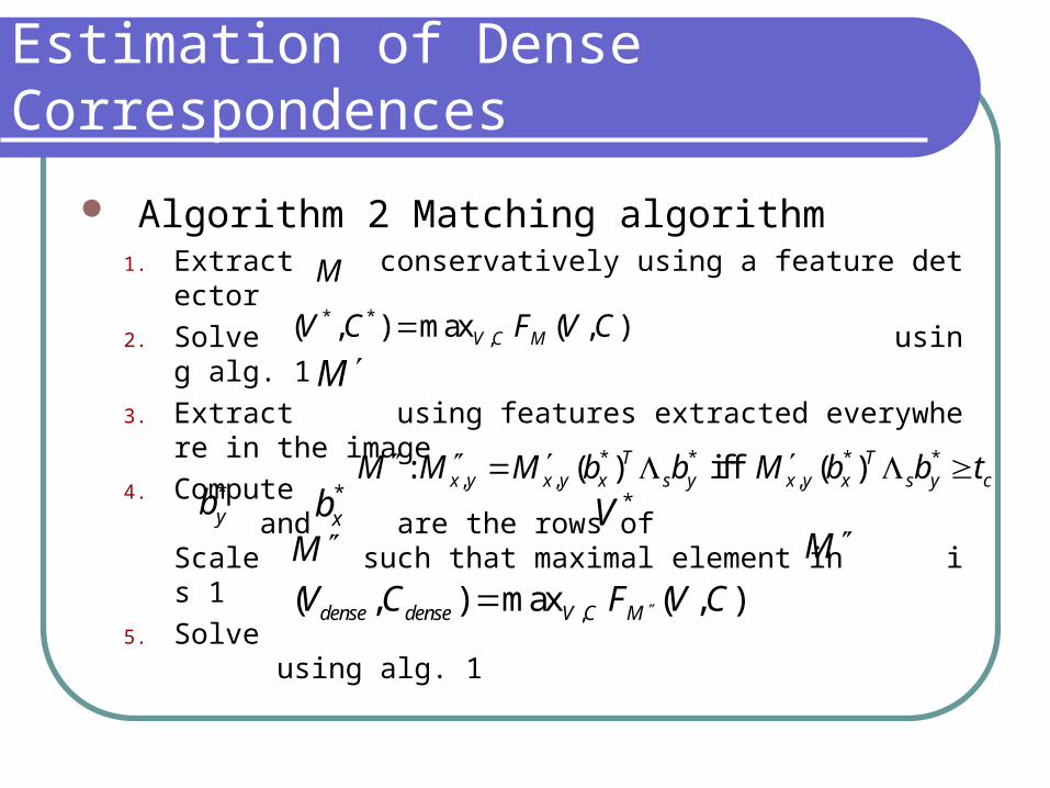
Algorithm 2 Matching algorithm1. Extract conservatively using a feature detector

2. Solve using alg. 1

3. Extract using features extracted everywhere in the image

4. Compute and are the rows of Scale such that maximal element in is 1

5. Solve using alg. 1

* *,( , ) max ( , )V C MV C F V C

M

* * * *, , ,: ( ) iff ( )T Tx y x y x s y x y x s y cM M M b b M b b t

*yb

*xb *V

M M

,( , ) max ( , )dense dense V C MV C F V C

M

Outline


Implementation Details

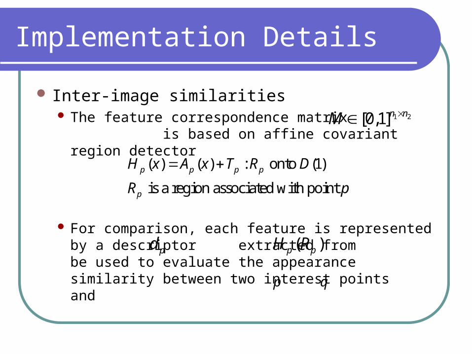
Inter-image similarities The feature correspondence matrix is

based on affine covariant region detector

For comparison, each feature is represented by a descriptor extracted frombe used to evaluate the appearance similarity between two interest points and

1 2[0,1]n nM

( ) ( ) : onto (1)

is a region associated with point

p p p p

p

H x A x T R D

R p

pd ( )p pH R

p q


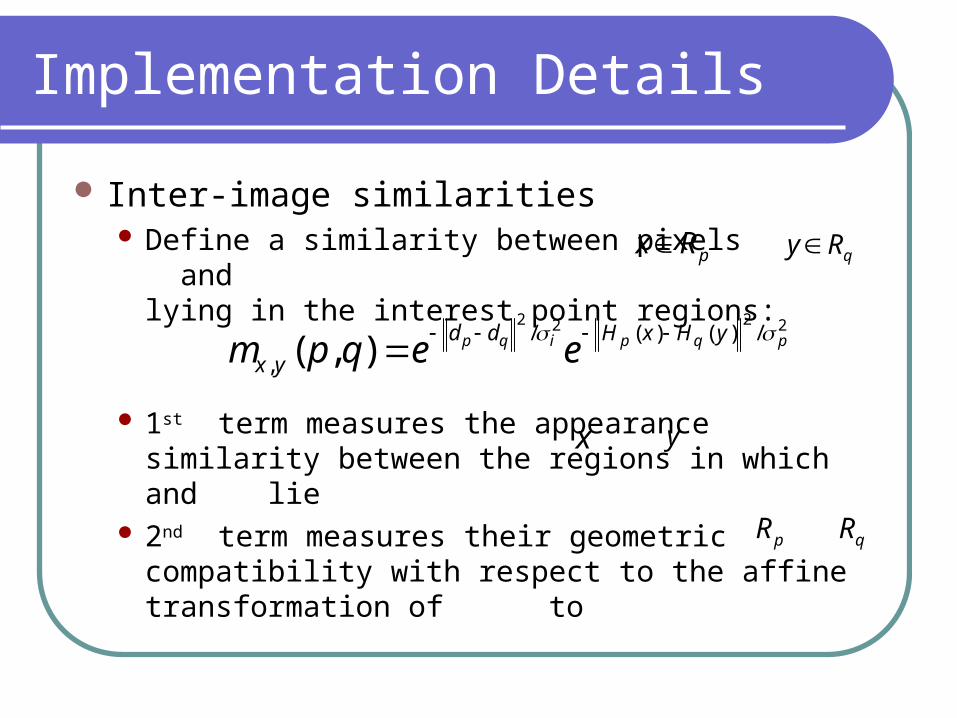
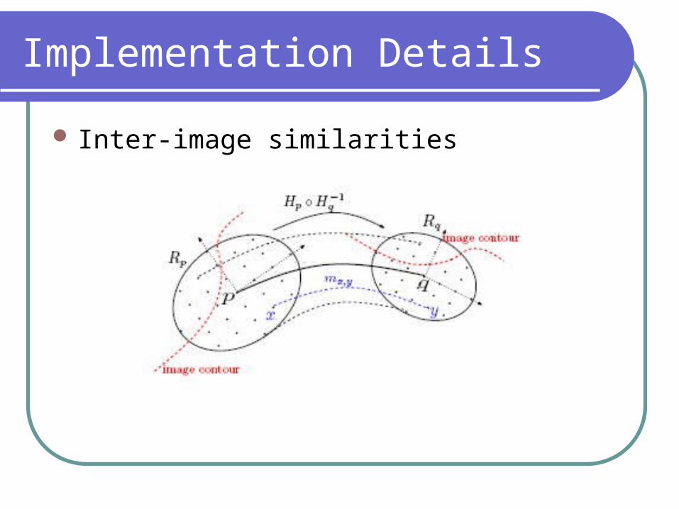
Inter-image similarities Define a similarity between pixels and

lying in the interest point regions:

1st term measures the appearance similarity between the regions in which and lie

2nd term measures their geometric compatibility with respect to the affine transformation of to

px R qy R

2 22 2/ ( ) ( ) /

, ( , ) p q i p q pd d H x H y

x ym p q e e

x y

pR qR


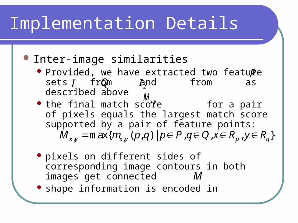
Inter-image similarities Provided, we have extracted two feature sets

from and from as described above the final match score for a pair of pixels equals

the largest match score supported by a pair of feature points:

pixels on different sides of corresponding image contours in both images get connected

shape information is encoded in

P1I Q 2I

,x yM

, ,max{ ( , ) | , , , }x y x y p qM m p q p P q Q x R y R

M


Inter-image similarities


Inter-image similarities The final is obtained by pruning:

retain

For feature extraction we use the MSER detector[12] combined with SIFT descriptor[4]

For the dense correspondences we use features extracted on a dense grid in the image and use the same descriptor

M

, , for , otherwise 0

where is a threshold

x y x y c

c

M M t

t

[10] T. Tuytelaars and L. V. Gool. Matching widely separated views based on affine invariant regions. IJCV, 59(1):61–85,2004[4] D. Lowe. Distinctive image features from scale-invariant keypoints. IJCV, 60(2), 91-110, 2004

M


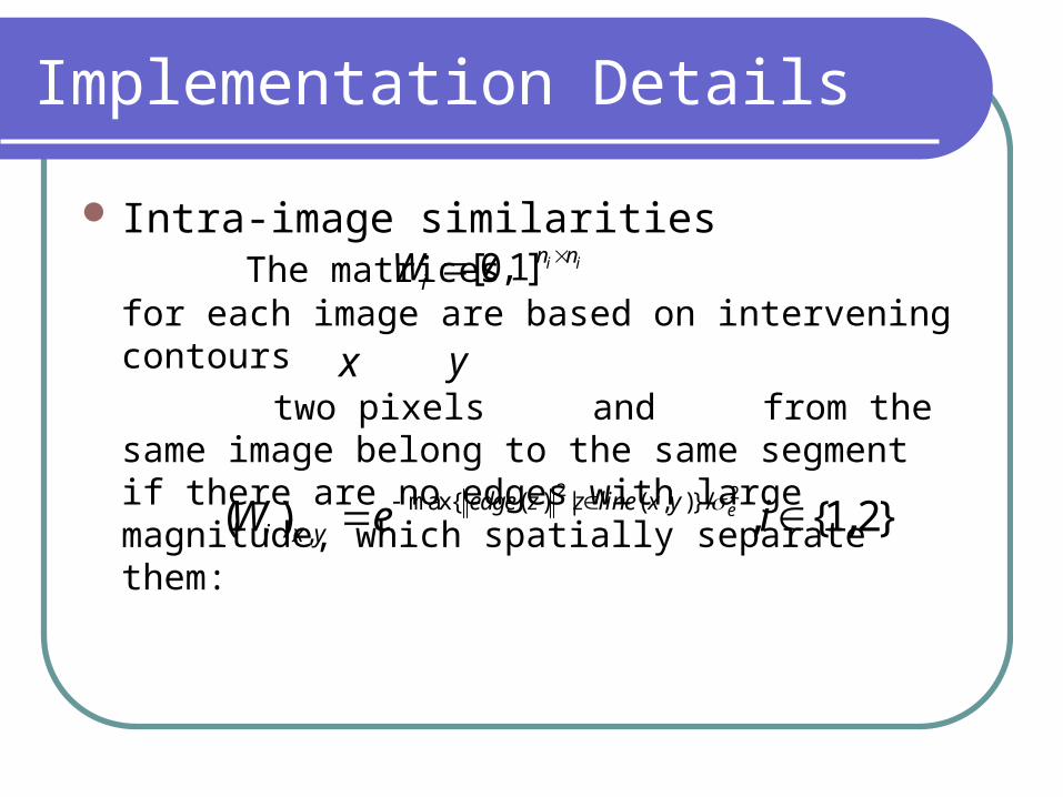
Intra-image similarities The matrices for each image are based on intervening contours

two pixels and from the same image belong to the same segment if there are no edges with large magnitude, which spatially separate them:

[0,1] i in niW

x y

2 2max{ ( ) | ( , )}/,( ) , {1,2}eedge z z line x y

i x yW e i


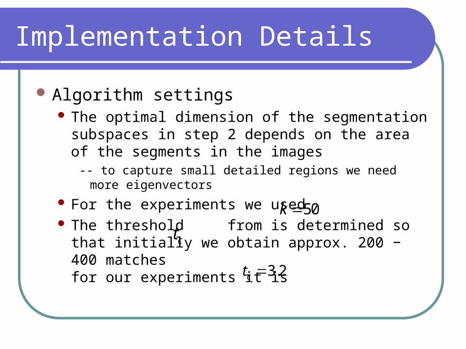
Algorithm settings The optimal dimension of the segmentation

subspaces in step 2 depends on the area of the segments in the images

-- to capture small detailed regions we need more eigenvectors

For the experiments we used The threshold from is determined so that initially

we obtain approx. 200 − 400 matchesfor our experiments it is

50k

ct

3.2ct


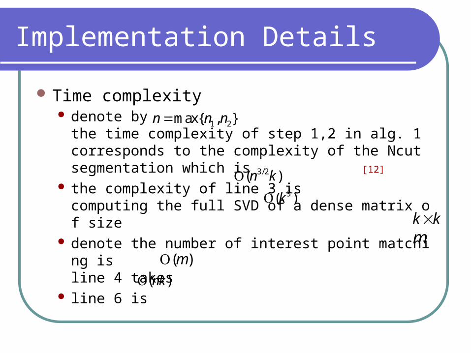
Time complexity denote by

the time complexity of step 1,2 in alg. 1 corresponds to the complexity of the Ncut segmentation which is [12]

the complexity of line 3 is computing the full SVD of a dense matrix of size

denote the number of interest point matching isline 4 takes

line 6 is

1 2max{ , }n n n

3/2( )n k

k k

3( )k

m( )m

( )nk


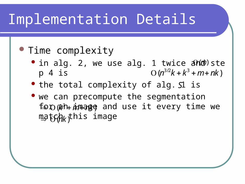
Time complexity in alg. 2, we use alg. 1 twice and step 4 is the total complexity of alg. 1 is we can precompute the segmentation for an ima

ge and use it every time we match this image

( )m3/2 3( )n k k m nk

S

3( )

( )

k m nk

nk

Outline


Experiments

We conduct two experiments: 1. detection of matching regions

2. place recognition datasets :

ICCV2005 Computer Vision Contest : Test4 & Final5

containing each 38 and 29 images of buildings each building is shown under different viewpoints

Experiments

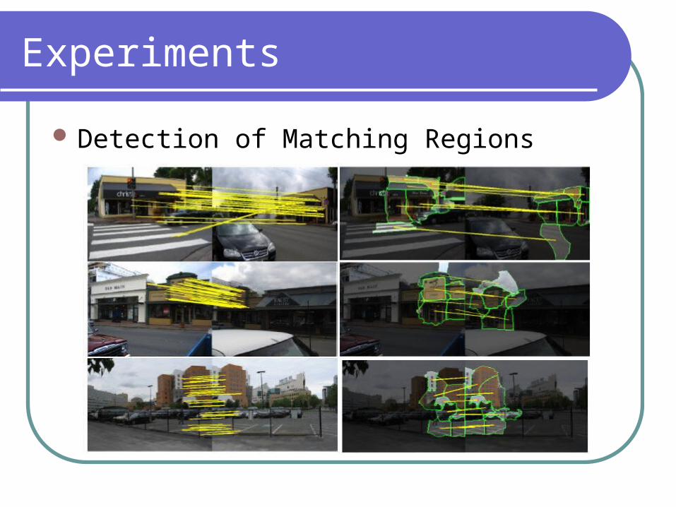
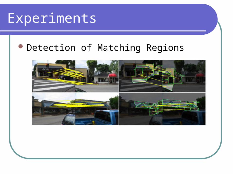
Detection of Matching Regions

Experiments


Experiments

Detection of Matching Regions detect matching regions, enhance the feature

matches, and segment common objects in manually selected image pairs

the 30 matches with highest score in of the output

the top 6 matching regions

denseC

Experiments


Finding the correct match for a given point may fail usually because :

1. The appearance similarity to the matching point is not as high as the score of the best matches ( not ranked high in the initial )

2. There are several matches with high scores due to similar or repeating structure

C

Experiments

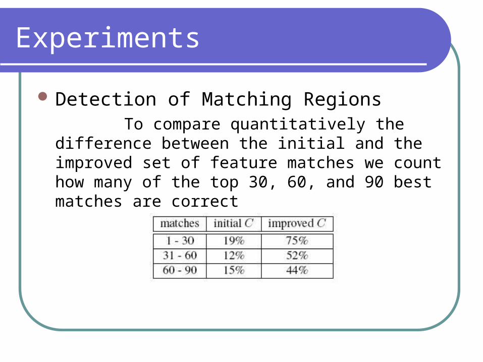
Detection of Matching Regions To compare quantitatively the difference between

the initial and the improved set of feature matches we count how many of the top 30, 60, and 90 best matches are correct

Experiments

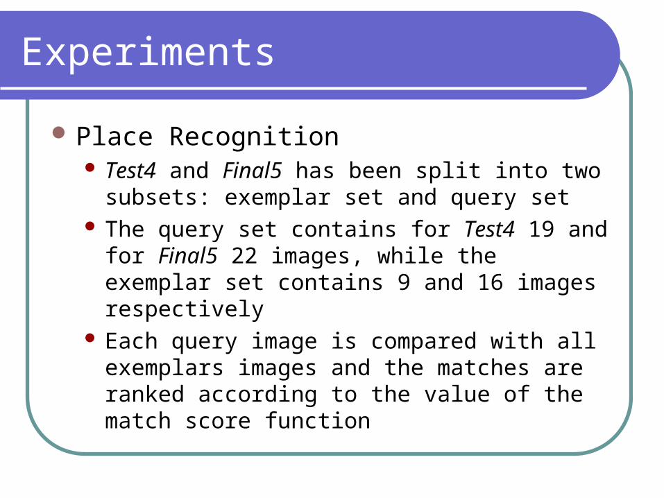
Place Recognition Test4 and Final5 has been split into two subsets:

exemplar set and query set The query set contains for Test4 19 and for Final5

22 images, while the exemplar set contains 9 and 16 images respectively

Each query image is compared with all exemplars images and the matches are ranked according to the value of the match score function

Experiments

Place Recognition For all queries, which have at least similar

exemplars in the datasetcompute how many of them are among the top matches

k

k

Outline


Conclusion

Present an algorithm to detects co-salient regions These regions are obtained through synchronization of

the segmentations using local feature matches Dense correspondence between coherent segments

are obtained The approach has shown promising results for

correspondence detection in the context of place recognition

Documents

Image Matching via Saliency Region Correspondences Alexander Toshev Jianbo Shi Kostas Daniilidis IEEE Conference on Computer Vision and Pattern Recognition