Image Morphing(4541.762 Computational Photography)

Jehee Lee

Seoul National University

With a lot of slides stolen from Alexei Efros and Seungyong Lee

Morphing = Object Averaging

• The aim is to find “an average” between two objects– Not an average of two images of objects…– …but an image of the average object!– How can we make a smooth transition in time?

• Do a “weighted average” over time t

• How do we know what the average object looks like?– We haven’t a clue!– But we can often fake something reasonable

• Usually required user/artist input

P

Qv = Q - P

P + 0.5v= P + 0.5(Q – P)= 0.5P + 0.5 Q

P + 1.5v= P + 1.5(Q – P)= -0.5P + 1.5 Q(extrapolation)Linear Interpolation

(Affine Combination):New point aP + bQ,defined only when a+b = 1So aP+bQ = aP+(1-a)Q

Averaging Points

• P and Q can be anything:– points on a plane (2D) or in space (3D)

– Colors in RGB or HSV (3D)

– Whole images (m-by-n D)… etc.

What’s the averageof P and Q?

Idea #1: Cross-Dissolve

• Interpolate whole images:

• Imagehalfway = (1-t)*Image1 + t*image2

• This is called cross-dissolve in film industry

• But what is the images are not aligned?

Idea #2: Align, then cross-disolve

• Align first, then cross-dissolve– Alignment using global warp – picture still valid

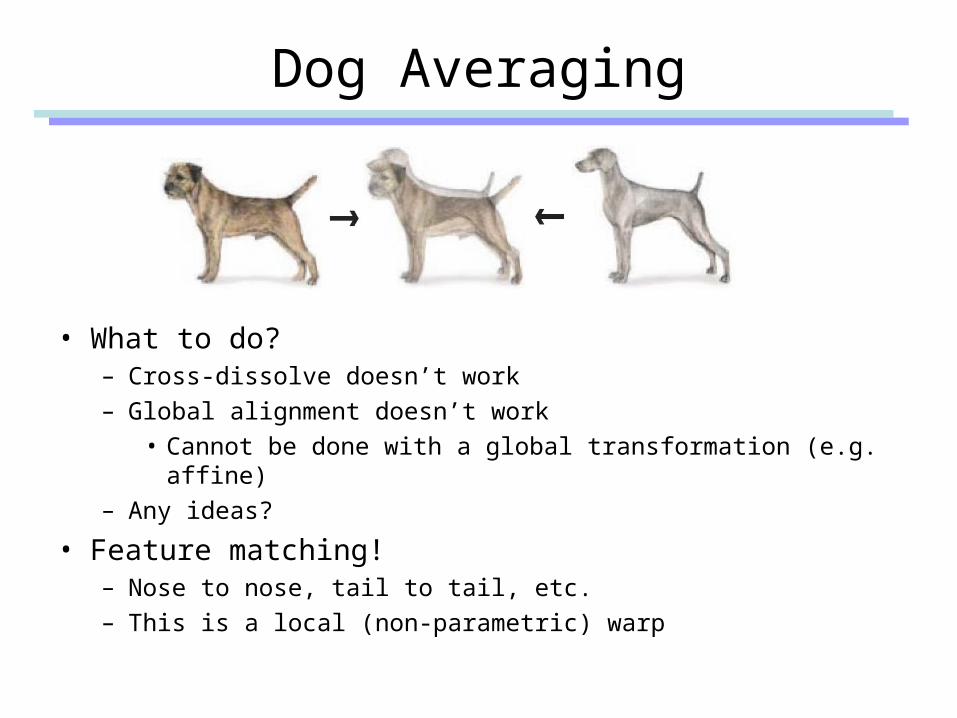
Dog Averaging

• What to do?– Cross-dissolve doesn’t work– Global alignment doesn’t work

• Cannot be done with a global transformation (e.g. affine)– Any ideas?

• Feature matching!– Nose to nose, tail to tail, etc.– This is a local (non-parametric) warp

Idea #3: Local warp, then cross-dissolve

Morphing procedure: for every t,1. Find the average shape (the “mean dog”)

– local warping

2. Find the average color– Cross-dissolve the warped images

Local (non-parametric) Image Warping

• Need to specify a more detailed warp function– Global warps were functions of a few (2,4,8) parameters– Non-parametric warps u(x,y) and v(x,y) can be defined independ

ently for every single location x,y!– Once we know vector field u,v we can easily warp each pixel (us

e backward warping with interpolation)

Image Warping – non-parametric

• Move control points to specify a spline warp• Spline produces a smooth vector field

Warp specification - dense

• How can we specify the warp?Specify corresponding spline control points

• interpolate to a complete warping function

But we want to specify only a few points, not a grid

Warp specification - sparse

• How can we specify the warp?Specify corresponding points

• interpolate to a complete warping function• How do we do it?

How do we go from feature points to pixels?

Triangular Mesh

1. Input correspondences at key feature points

2. Define a triangular mesh over the points– Same mesh in both images!– Now we have triangle-to-triangle correspondences

3. Warp each triangle separately from source to destination– How do we warp a triangle?– 3 points = affine warp!– Just like texture mapping

Triangulations

• A triangulation of set of points in the plane is a partition of the convex hull to triangles whose vertices are the points, and do not contain other points.

• There are an exponential number of triangulations of a point set.

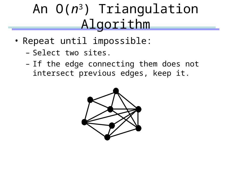
An O(n3) Triangulation Algorithm

• Repeat until impossible:– Select two sites.– If the edge connecting them does not intersect

previous edges, keep it.

“Quality” Triangulations

• Let (T) = (1, 2 ,.., 3t) be the vector of angles in the triangulation T in increasing order.

• A triangulation T1 will be “better” than T2 if (T1) > (T

2) lexicographically.• The Delaunay triangulation is the “best”

– Maximizes smallest angles

good bad

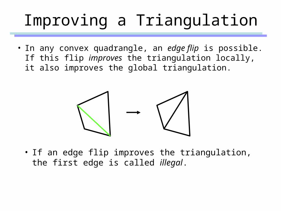
Improving a Triangulation

• In any convex quadrangle, an edge flip is possible. If this flip improves the triangulation locally, it also improves the global triangulation.

• If an edge flip improves the triangulation, the first edge is called illegal.

Illegal Edges• Lemma: An edge pq is illegal iff one of its opposite vertices is in

side the circle defined by the other three vertices.• Proof: By Thales’ theorem.

• Theorem: A Delaunay triangulation does not contain illegal edges.• Corollary: A triangle is Delaunay iff the circle through its vertices is empty of other sites.• Corollary: The Delaunay triangulation is not unique if more than three sites are co-circular.

p

q

Naïve Delaunay Algorithm

• Start with an arbitrary triangulation. Flip any illegal edge until no more exist.

• Could take a long time to terminate.

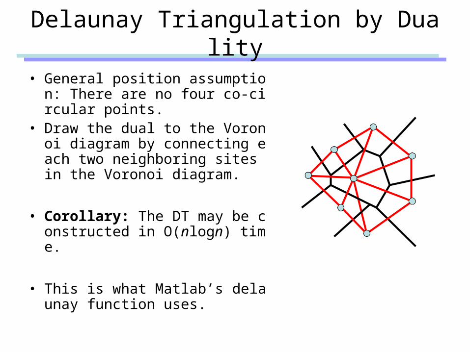
Delaunay Triangulation by Duality

• General position assumption: There are no four co-circular points.

• Draw the dual to the Voronoi diagram by connecting each two neighboring sites in the Voronoi diagram.

• Corollary: The DT may be constructed in O(nlogn) time.

• This is what Matlab’s delaunay function uses.

Image Morphing

• We know how to warp one image into the other, but how do we create a morphing sequence?

1. Create an intermediate shape (by interpolation)

2. Warp both images towards it

3. Cross-dissolve the colors in the newly warped images

Warp interpolation

• How do we create an intermediate warp at time t?– Assume t = [0,1]– Simple linear interpolation of each feature pair– (1-t)*p1+t*p0 for corresponding features p0 and p1

Other Issues

• Beware of folding– You are probably trying to do something 3D-ish

• Morphing can be generalized into 3D– If you have 3D data, that is!

• Extrapolation can sometimes produce interesting effects– Caricatures

23

Image Metamorphosis

• Uniform Transition

24

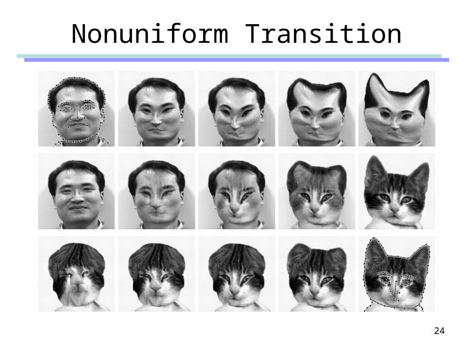
Nonuniform Transition

Dynamic Scene

26

Warp Generation (7)

destination

• Scattered Data Interpolation – Scattered points for specifying features– Point sampling of polylines, curves and graphs– Convenient feature specification– Precise, smooth, and intuitive warps– Various methods

source

27

•Surface Construction – Basic idea

• construct two surfaces for x- and y-components• W(u, v) = (X(u, v), Y(u, v))

• X(u, v) = u + X(u, v), Y(u, v) = v + Y(u, v)

• X(uk, vk) = Xk = xk uk

• Y(uk, vk) = yk = yk vk

X(u, v)

(u, v)

Warp Generation (8)

source destination

W

(uk, vk)(xk, vk)

28

Warp Generation (9)

• Surface Construction (2)– Thin plate spline

• requirements– positional constraints– smoothness

• minimize

• numerical solution– Results

– precise and C1-continuous warps– intuitive distortions

f(u, v)

(u, v)

E ff

u

f

u v

f

vdudv f u v xk k k

k

( ) ( ( , ) )

2

2

2 2 2 2

2

2

22

29

Warp Generation (11)

• Energy Minimization (2)– Numerical solution

• variational derivative: a differential equation• finite differencing: a nonlinear system• diffusion equation: an equilibrium solution• differencing with time: a sequence of equations• multigrid relaxation method

– Result• precise, C1-continuous, and one-to-one warps• natural and Intuitive distortions

Radial Basis Functions

• Radial refers to the pattern that you get when straight lines are drawn from the center of a circle to a number of points round the edge

• Radial basis function – A real valued function

– having a center in a parameter space

– The function value is determined by a distance from the center

:

Ni x

ixx

Scattered Data Interpolation using RBF

• Find a function that interpolate given points such that

• RBF interpolation

– We use n basis functions (same as # of given data points)– We don’t have a grid structure (compare to tensor-product

surfaces)– Radial basis function is easily defined in any dimensional spaces

N:)S(x}1|),{( nihii x ih ii allfor )S(x

n

jjj

1

)()S( xxx

Scattered Data Interpolation using RBF

• RBF interpolation as a linear system

n

jjj

1

)()S( xxx

nnnnn

n

n

h

h

h

)()()S(

)()()S(

)()()S(

1

22212

11111

xxxxx

xxxxx

xxxxx

Scattered Data Interpolation using RBF

• RBF interpolation as a linear system

n

jjj

1

)()S( xxx

nnnn h

h

h

2

1

2

1

22

11

)()(

)()(

)()(

xxxx

xxxx

xxxx

Popular Choices for RBF

• Thin-Plate

• Multiquadric

• Gaussian

• Biharmonic

• Triharmonic

• See demo: RBFwithoutLinearApproximation.exe

rrr log2

22 crr

rr

3rr

)exp( 2crr

for some constant c

for some constant c

Augmented Polynomial Function

• A linear function or a low-order polynomial is augmented for better extrapolation

• Under-specified linear system is obtained• Orthogonality conditions give a unique solution

M

jjjP

1

)()()S( xxxx

zcycxcczyxP

ycxccyxP

3210

210

),,( 3D,In

),( 2D,In

Demo

• Using orthogonality conditions– RBF.exe

• Using pseudo inverse– RBFpseudoInverse.exe

Programming Assignment #2 (Image Morphing)

• Requirements– Create a sequence of your face images that morphs

into another person– Implement your own choice of warping methods

• Optional– User interfaces for specifying correspondences

between images are not mandatory. Do it for your own fun

– You can create a movie file