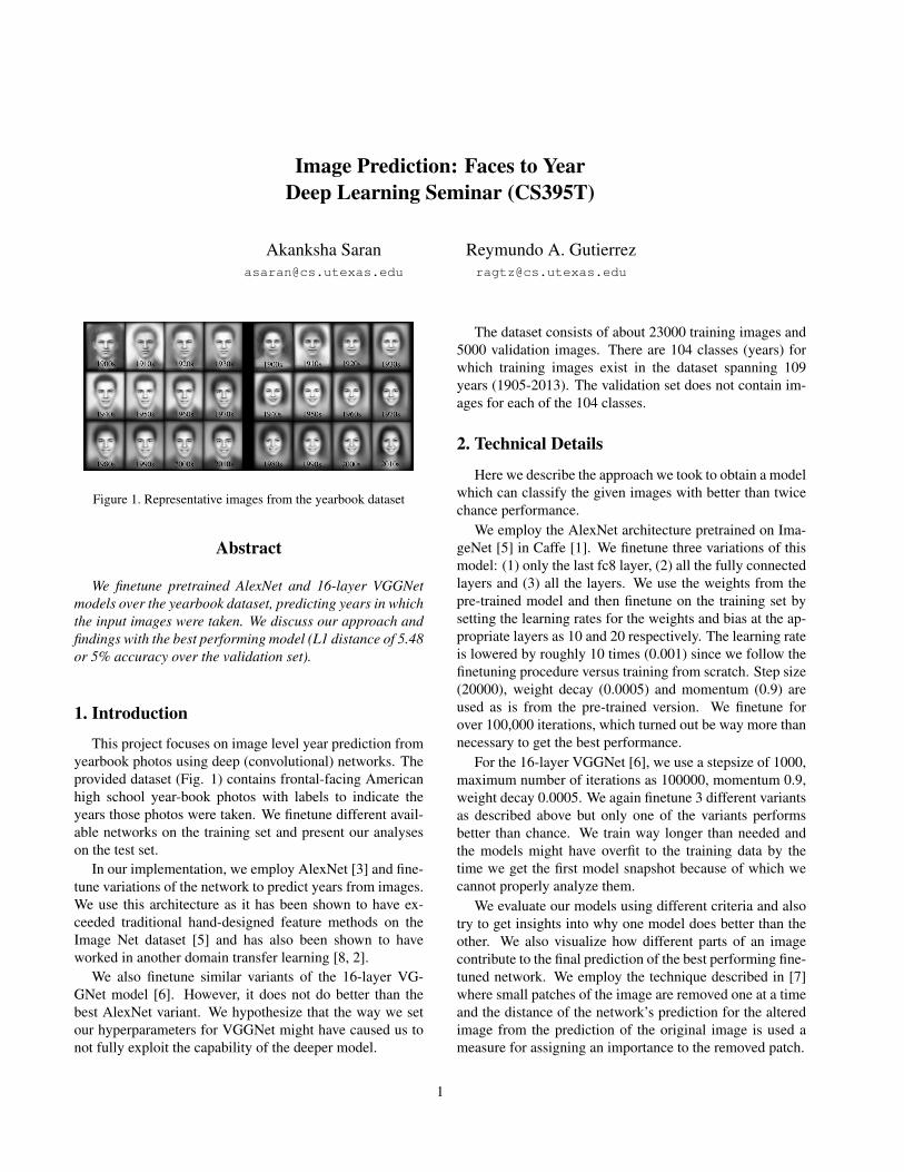
Image Prediction: Faces to YearDeep Learning Seminar (CS395T)

Akanksha Saranasaran@cs.utexas.edu

Reymundo A. Gutierrezragtz@cs.utexas.edu

Figure 1. Representative images from the yearbook dataset

Abstract

We finetune pretrained AlexNet and 16-layer VGGNetmodels over the yearbook dataset, predicting years in whichthe input images were taken. We discuss our approach andfindings with the best performing model (L1 distance of 5.48or 5% accuracy over the validation set).

1. Introduction

This project focuses on image level year prediction fromyearbook photos using deep (convolutional) networks. Theprovided dataset (Fig. 1) contains frontal-facing Americanhigh school year-book photos with labels to indicate theyears those photos were taken. We finetune different avail-able networks on the training set and present our analyseson the test set.

In our implementation, we employ AlexNet [3] and fine-tune variations of the network to predict years from images.We use this architecture as it has been shown to have ex-ceeded traditional hand-designed feature methods on theImage Net dataset [5] and has also been shown to haveworked in another domain transfer learning [8, 2].

We also finetune similar variants of the 16-layer VG-GNet model [6]. However, it does not do better than thebest AlexNet variant. We hypothesize that the way we setour hyperparameters for VGGNet might have caused us tonot fully exploit the capability of the deeper model.

The dataset consists of about 23000 training images and5000 validation images. There are 104 classes (years) forwhich training images exist in the dataset spanning 109years (1905-2013). The validation set does not contain im-ages for each of the 104 classes.

2. Technical Details

Here we describe the approach we took to obtain a modelwhich can classify the given images with better than twicechance performance.

We employ the AlexNet architecture pretrained on Ima-geNet [5] in Caffe [1]. We finetune three variations of thismodel: (1) only the last fc8 layer, (2) all the fully connectedlayers and (3) all the layers. We use the weights from thepre-trained model and then finetune on the training set bysetting the learning rates for the weights and bias at the ap-propriate layers as 10 and 20 respectively. The learning rateis lowered by roughly 10 times (0.001) since we follow thefinetuning procedure versus training from scratch. Step size(20000), weight decay (0.0005) and momentum (0.9) areused as is from the pre-trained version. We finetune forover 100,000 iterations, which turned out be way more thannecessary to get the best performance.

For the 16-layer VGGNet [6], we use a stepsize of 1000,maximum number of iterations as 100000, momentum 0.9,weight decay 0.0005. We again finetune 3 different variantsas described above but only one of the variants performsbetter than chance. We train way longer than needed andthe models might have overfit to the training data by thetime we get the first model snapshot because of which wecannot properly analyze them.

We evaluate our models using different criteria and alsotry to get insights into why one model does better than theother. We also visualize how different parts of an imagecontribute to the final prediction of the best performing fine-tuned network. We employ the technique described in [7]where small patches of the image are removed one at a timeand the distance of the network’s prediction for the alteredimage from the prediction of the original image is used ameasure for assigning an importance to the removed patch.

1

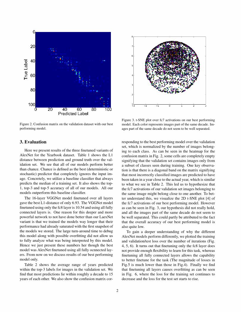
Figure 2. Confusion matrix on the validation dataset with our bestperforming model.

3. Evaluation

Here we present results of the three finetuned variants ofAlexNet for the Yearbook dataset. Table 1 shows the L1distance between prediction and ground truth over the val-idation set. We see that all of our models perform betterthan chance. Chance is defined as the best (deterministic orstochastic) predictor that completely ignores the input im-age. Concretely, we utilize a baseline classifier that alwayspredicts the median of a training set. It also shows the top-1, top-3 and top-5 accuracy of all of our models. All ourmodels outperform this baseline classifier.

The 16-layer VGGNet model finetuned over all layersgave the best L1-distance of only 6.93. The VGGNet modelfinetuned using only the fc8 layer is 10.54 and using all fullyconnected layers is. One reason for this deeper and morepowerful network to not have done better than our LaexNetvariant is that we trained the models way longer that theirperformance had already saturated with the first snapshot ofthe models we stored. The large turn-around time to debugthis model along with possible overfitting did not allow usto fully analyze what was being interpreted by this model.Hence we just present these numbers her though the bestmodel was AlexNet finetuned using all fully ocnnected lay-ers. From now on we discuss results of our best performingmodel only.

Table 2 shows the average range of years predictedwithin the top-3 labels for images in the validation set. Wefind that most predictions lie within roughly a decade to 15years of each other. We also show the confusion matrix cor-

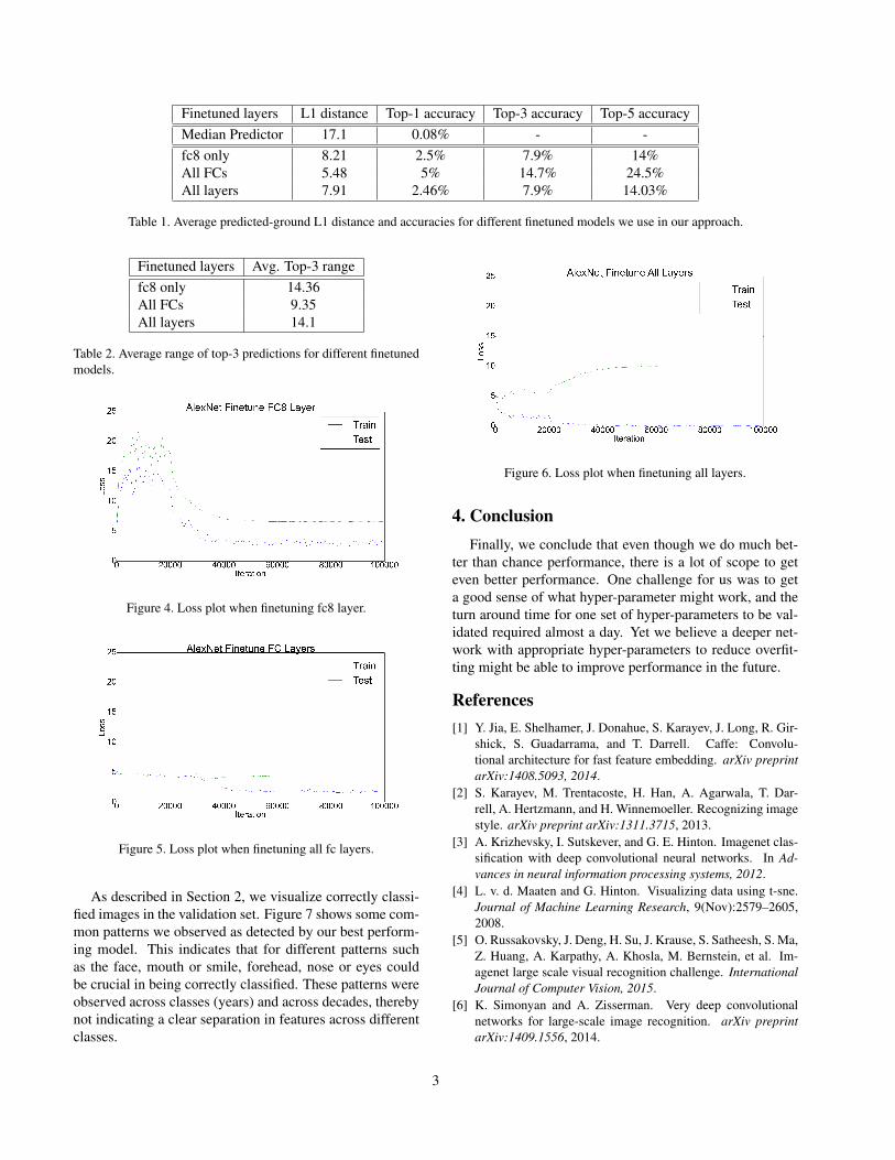
Figure 3. t-SNE plot over fc7 activations on our best performingmodel. Each color represents images part of the same decade. Im-ages part of the same decade do not seem to be well separated.

responding to the best performing model over the validationset, which is normalized by the number of images belong-ing to each class. As can be seen in the heatmap for theconfusion matrix in Fig. 2, some cells are completely emptysignifying that the validation set contains images only froma subset of classes seen during training. One key observa-tion is that there is a diagonal band on the matrix signifyingthat most incorrectly classified images are predicted to havebeen taken in a year close to the actual year, which is similarto what we see in Table 2. This led us to hypothesize thatthe fc7 activations of our validation set images belonging tothe same image might belong close to one another. To bet-ter understand this, we visualize the 2D t-SNE plot [4] ofthe fc7 activations of our best performing model. Howeveras can be seen in Fig. 3, our hypothesis did not really hold,and all the images part of the same decade do not seem tobe well separated. This could partly be attributed to the factthat the overall accuracy of our best performing model isalso quite low.

To gain a deeper understanding of why the differentAlexNet models perform differently, we plotted the trainingand validation/test loss over the number of iterations (Fig.4, 5, 6). It turns out that finetuning only the fc8 layer doesnot provide enough flexibility to learn for this task, whereasfinetuning all fully connected layers allows the capabilityto better finetune for the task (The magnitude of losses inFig.5 is much lower than those in Fig.4). Finally we findthat finetuning all layers causes overfitting as can be seenin Fig. 6, where the loss for the training set continues todecrease and the loss for the test set starts to rise.

2

Finetuned layers L1 distance Top-1 accuracy Top-3 accuracy Top-5 accuracyMedian Predictor 17.1 0.08% - -fc8 only 8.21 2.5% 7.9% 14%All FCs 5.48 5% 14.7% 24.5%All layers 7.91 2.46% 7.9% 14.03%

Table 1. Average predicted-ground L1 distance and accuracies for different finetuned models we use in our approach.

Finetuned layers Avg. Top-3 rangefc8 only 14.36All FCs 9.35All layers 14.1

Table 2. Average range of top-3 predictions for different finetunedmodels.

Figure 4. Loss plot when finetuning fc8 layer.

Figure 5. Loss plot when finetuning all fc layers.

As described in Section 2, we visualize correctly classi-fied images in the validation set. Figure 7 shows some com-mon patterns we observed as detected by our best perform-ing model. This indicates that for different patterns suchas the face, mouth or smile, forehead, nose or eyes couldbe crucial in being correctly classified. These patterns wereobserved across classes (years) and across decades, therebynot indicating a clear separation in features across differentclasses.

Figure 6. Loss plot when finetuning all layers.

4. ConclusionFinally, we conclude that even though we do much bet-

ter than chance performance, there is a lot of scope to geteven better performance. One challenge for us was to geta good sense of what hyper-parameter might work, and theturn around time for one set of hyper-parameters to be val-idated required almost a day. Yet we believe a deeper net-work with appropriate hyper-parameters to reduce overfit-ting might be able to improve performance in the future.

References[1] Y. Jia, E. Shelhamer, J. Donahue, S. Karayev, J. Long, R. Gir-

shick, S. Guadarrama, and T. Darrell. Caffe: Convolu-tional architecture for fast feature embedding. arXiv preprintarXiv:1408.5093, 2014.

[2] S. Karayev, M. Trentacoste, H. Han, A. Agarwala, T. Dar-rell, A. Hertzmann, and H. Winnemoeller. Recognizing imagestyle. arXiv preprint arXiv:1311.3715, 2013.

[3] A. Krizhevsky, I. Sutskever, and G. E. Hinton. Imagenet clas-sification with deep convolutional neural networks. In Ad-vances in neural information processing systems, 2012.

[4] L. v. d. Maaten and G. Hinton. Visualizing data using t-sne.Journal of Machine Learning Research, 9(Nov):2579–2605,2008.

[5] O. Russakovsky, J. Deng, H. Su, J. Krause, S. Satheesh, S. Ma,Z. Huang, A. Karpathy, A. Khosla, M. Bernstein, et al. Im-agenet large scale visual recognition challenge. InternationalJournal of Computer Vision, 2015.

[6] K. Simonyan and A. Zisserman. Very deep convolutionalnetworks for large-scale image recognition. arXiv preprintarXiv:1409.1556, 2014.

3

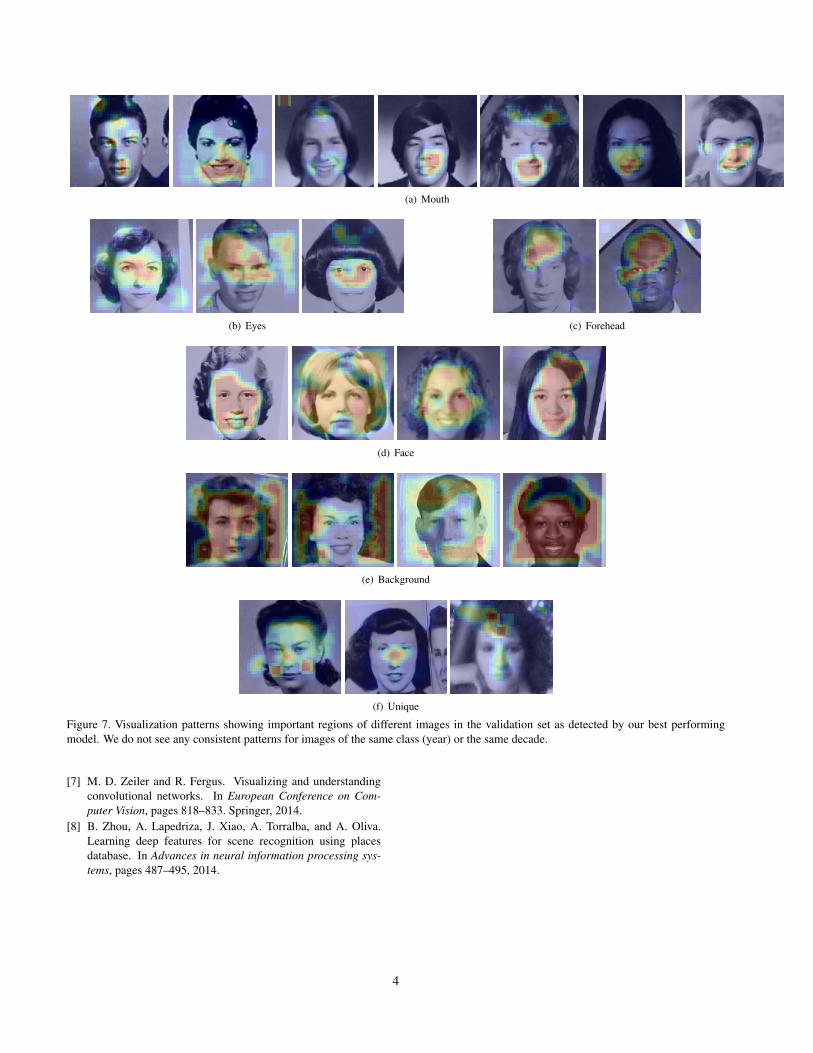
(a) Mouth

(b) Eyes (c) Forehead

(d) Face

(e) Background

(f) Unique

Figure 7. Visualization patterns showing important regions of different images in the validation set as detected by our best performingmodel. We do not see any consistent patterns for images of the same class (year) or the same decade.

[7] M. D. Zeiler and R. Fergus. Visualizing and understandingconvolutional networks. In European Conference on Com-puter Vision, pages 818–833. Springer, 2014.

[8] B. Zhou, A. Lapedriza, J. Xiao, A. Torralba, and A. Oliva.Learning deep features for scene recognition using placesdatabase. In Advances in neural information processing sys-tems, pages 487–495, 2014.

4