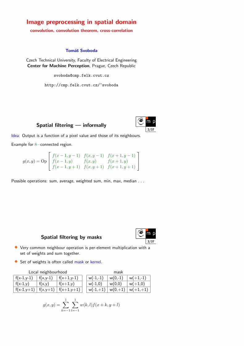
Image preprocessing in spatial domainconvolution, convolution theorem, cross-correlation

Tomas Svoboda

Czech Technical University, Faculty of Electrical Engineering

Center for Machine Perception, Prague, Czech Republic

svoboda@cmp.felk.cvut.cz

http://cmp.felk.cvut.cz/~svoboda

2/37Spatial filtering — informally

Idea: Output is a function of a pixel value and those of its neighbours.

Example for 8−connected region.

g(x, y) = Op

f(x− 1, y − 1) f(x, y − 1) f(x + 1, y − 1)f(x− 1, y) f(x, y) f(x + 1, y)f(x− 1, y + 1) f(x, y + 1) f(x + 1, y + 1)

Possible operations: sum, average, weighted sum, min, max, median . . .

3/37Spatial filtering by masks

� Very common neighbour operation is per-element multiplication with a

set of weights and sum together.

� Set of weights is often called mask or kernel.

Local neighbourhood mask

f(x-1,y-1) f(x,y-1) f(x+1,y-1)

f(x-1,y) f(x,y) f(x+1,y)

f(x-1,y+1) f(x,y+1) f(x+1,y+1)

w(-1,-1) w(0,-1) w(+1,-1)

w(-1,0) w(0,0) w(+1,0)

w(-1,+1) w(0,+1) w(+1,+1)

g(x, y) =1∑

k=−1

1∑l=−1

w(k, l)f(x + k, y + l)

4/372D convolution

� Spatial filtering is often referred to as convolution.

� We say, we convolve the image by a kernel or mask.

� Though, it is not the same. Convolution uses a flipped kernel.

Local neighbourhood mask

f(x-1,y-1) f(x,y-1) f(x+1,y-1)

f(x-1,y) f(x,y) f(x+1,y)

f(x-1,y+1) f(x,y+1) f(x+1,y+1)

w(+1,+1) w(0,+1) w(-1,+1)

w(+1,0) w(0,0) w(-1,0)

w(+1,-1) w(0,-1) w(-1,-1)

g(x, y) =1∑

k=−1

1∑l=−1

w(k, l)f(x− k, y − l)

5/372D Convolution — Why is it important?

� Input and output signals need not to be related through convolution,

but if they are (and only if) the system is linear and time invariant.

� 2D convolution describes well the formation of images.

� Many image distortions made by imperfect acquisition may be modelled

by 2D convolution, too.

� It is a powerful thinking tool.

6/372D convolution — definition

Convolution integral

g(x, y) =∫ ∞

−∞

∫ ∞

−∞f(x− k, y − l)h(k, l)dkdl

Symbolic abbreviation

g(x, y) = f(x, y) ∗ h(x, y)

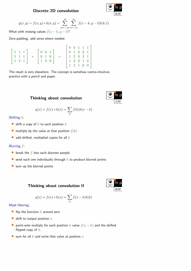
6/37Discrete 2D convolution

g(x, y) = f(x, y) ∗ h(x, y) =∞∑

k=−∞

∞∑l=−∞

f(x− k, y − l)h(k, l)

What with missing values f(x− k, y − l)?

Zero-padding: add zeros where needed.

1 1 11 1 11 2 1

∗

0 0 10 1 01 0 0

=

0 0 1 1 10 1 2 2 11 2 3 3 11 2 3 1 01 2 1 0 0

The result is zero elsewhere. The concept is somehow contra-intuitive,

practice with a pencil and paper.

7/37Thinking about convolution

g(x) = f(x) ∗ h(x) =∑

k

f(k)h(x− k)

Shifting h:

� shift a copy of h to each position k

� multiply by the value at that position f(k)

� add shifted, multiplied copies for all k

Blurring f :

� break the f into each discrete sample

� send each one individually through h to produce blurred points

� sum up the blurred points

8/37Thinking about convolution II

g(x) = f(x) ∗ h(x) =∑

k

f(x− k)h(k)

Mask filtering:

� flip the function h around zero

� shift to output position x

� point-wise multiply for each position k value f(x− k) and the shifted

flipped copy of h.

� sum for all k and write that value at position x

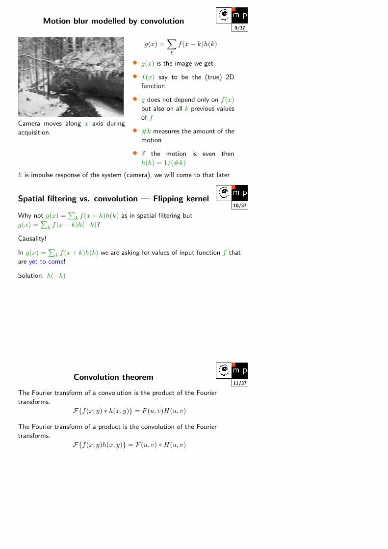
9/37Motion blur modelled by convolution

Camera moves along x axis during

acquisition.

g(x) =∑

k

f(x− k)h(k)

� g(x) is the image we get

� f(x) say to be the (true) 2D

function

� g does not depend only on f(x)but also on all k previous values

of f

� #k measures the amount of the

motion

� if the motion is even then

h(k) = 1/(#k)

h is impulse response of the system (camera), we will come to that later

10/37Spatial filtering vs. convolution — Flipping kernel

Why not g(x) =∑

k f(x + k)h(k) as in spatial filtering but

g(x) =∑

k f(x− k)h(−k)?

Causality!

In g(x) =∑

k f(x + k)h(k) we are asking for values of input function f that

are yet to come!

Solution: h(−k)

11/37Convolution theorem

The Fourier transform of a convolution is the product of the Fourier

transforms.

F{f(x, y) ∗ h(x, y)} = F (u, v)H(u, v)

The Fourier transform of a product is the convolution of the Fourier

transforms.

F{f(x, y)h(x, y)} = F (u, v) ∗H(u, v)

12/37Convolution theorem — proof

F{f(x, y) ∗ h(x, y)} = F (u, v)H(u, v)

F (u) = 1M

∑M−1x=0 f(x) exp (−i2πux/M) and g(x) =

∑M−1k=0 f(k)h(x− k)

F{g(x)} = . . .

� 1M

∑M−1x=0

∑M−1k=0 f(k)h(x− k)e(−i2πux/M)

� introduce new (dummy) variable w = x− k

� 1M

∑M−1k=0 f(k)

∑(M−1)−kw=−k h(w)e(−i2πu(w+k)/M)

� remember that all functions g, h, f are assumed to be periodic with

period M

� 1M

∑M−1k=0 f(k)e(−i2πuk/M)

∑M−1w=0 h(w)e(−i2πuw/M)

� which is indeed F (u)H(u)

13/37Convolution theorem — what is it good for?

� Direct relationship between filtering in spatial and frequency domain.

See few slides later.

� Image restoration, sometimes called deconvolution

� Speed of computation. Convolution has O(M2), Fast Fourier

Transform (FFT) has O(M log2 M)

Enough theory for now. Go for examples . . .

14/37Spatial filtering

What is it good for?

� smoothing

� sharpening

� noise removal

� edge detection

� pattern matching

� ...

15/37Smoothing

Output value is computed as an average of the input value and its

neighbourhood.

� Advantage: less noise

� Disadvantage: blurring

� Any kernel with all positive weights causes smoothing or blurring

� They are called low-pass filters (We know them already!)

Averaging:

g(x, y) =∑

k

∑l w(k, l)f(x + k, y + l)∑

k

∑l w(k, l)

16/37Smoothing kernels

Can be of any size, any shape

h =19

1 1 11 1 11 1 1

, h =116

1 2 12 4 21 2 1

,

h =125

1 1 1 1 11 1 1 1 11 1 1 1 11 1 1 1 11 1 1 1 1

.

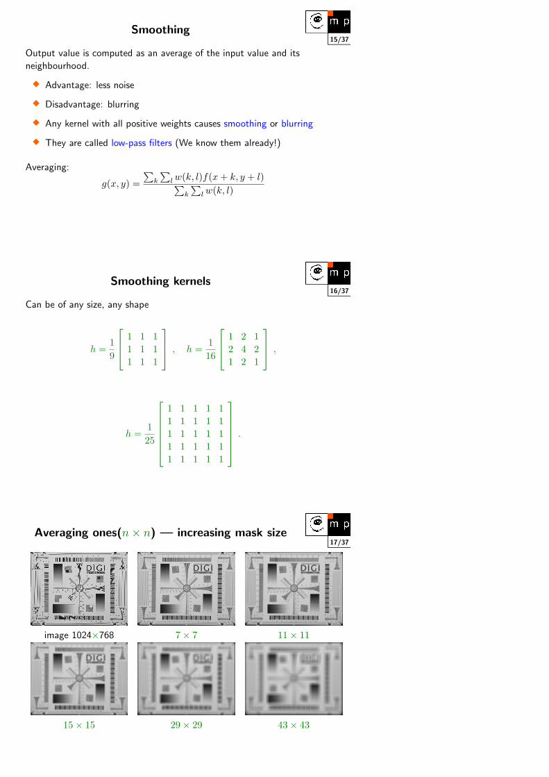
17/37Averaging ones(n× n) — increasing mask size

image 1024×768 7× 7 11× 11

15× 15 29× 29 43× 43

18/37

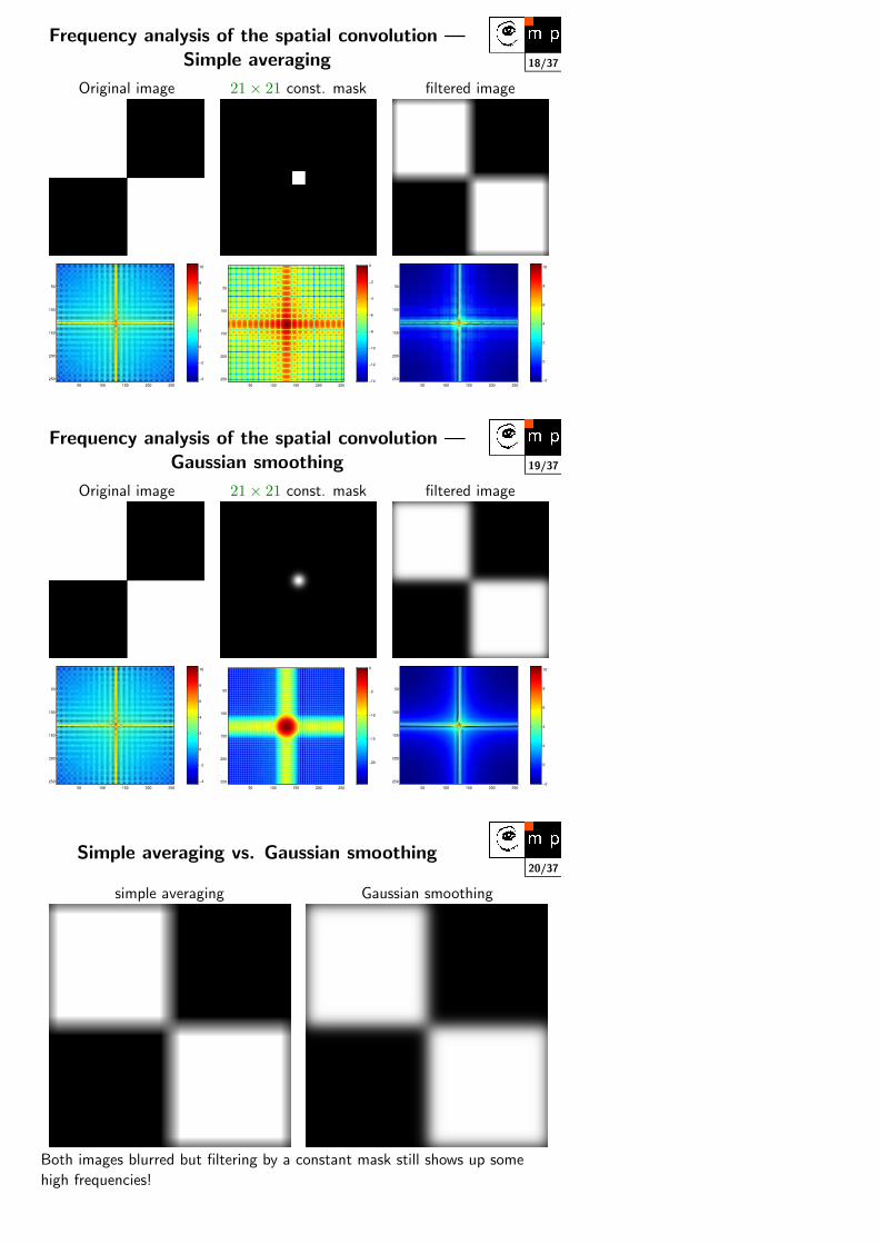
Frequency analysis of the spatial convolution —Simple averaging

Original image 21× 21 const. mask filtered image

50 100 150 200 250

50

100

150

200

250 −4

−2

0

2

4

6

8

10

50 100 150 200 250

50

100

150

200

250 −14

−12

−10

−8

−6

−4

−2

0

50 100 150 200 250

50

100

150

200

250 −2

0

2

4

6

8

10

19/37

Frequency analysis of the spatial convolution —Gaussian smoothing

Original image 21× 21 const. mask filtered image

50 100 150 200 250

50

100

150

200

250 −4

−2

0

2

4

6

8

10

50 100 150 200 250

50

100

150

200

250

−20

−15

−10

−5

0

50 100 150 200 250

50

100

150

200

250 −2

0

2

4

6

8

10

20/37Simple averaging vs. Gaussian smoothing

simple averaging Gaussian smoothing

Both images blurred but filtering by a constant mask still shows up some

high frequencies!

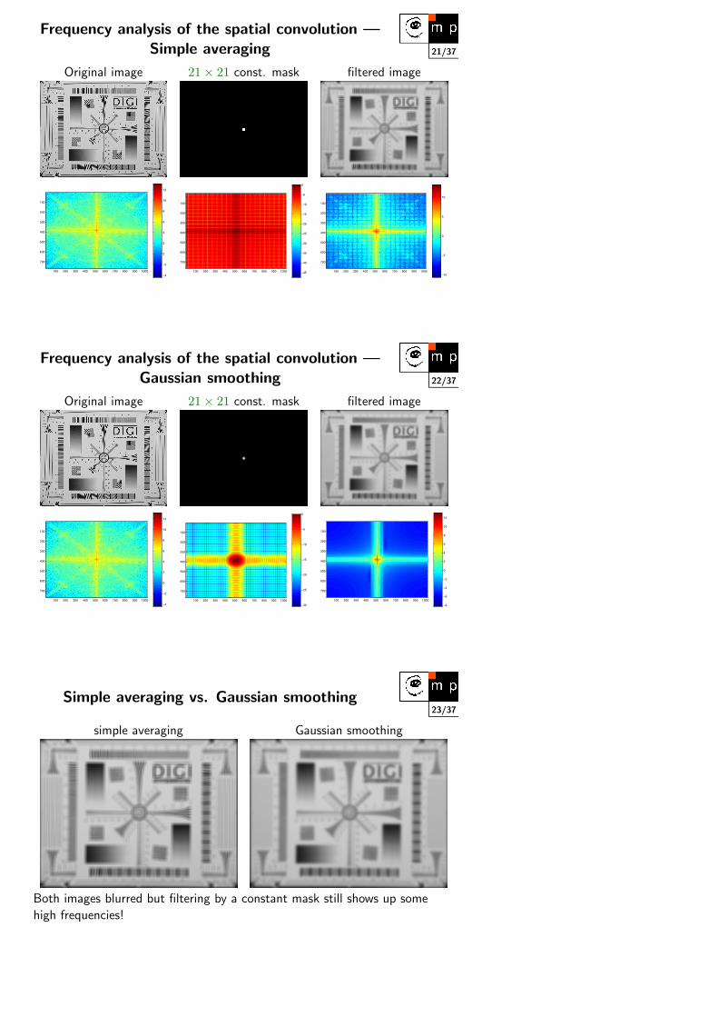
21/37

Frequency analysis of the spatial convolution —Simple averaging

Original image 21× 21 const. mask filtered image

100 200 300 400 500 600 700 800 900 1000

100

200

300

400

500

600

700

−4

−2

0

2

4

6

8

10

12

100 200 300 400 500 600 700 800 900 1000

100

200

300

400

500

600

700

−45

−40

−35

−30

−25

−20

−15

−10

−5

0

100 200 300 400 500 600 700 800 900 1000

100

200

300

400

500

600

700

−10

−5

0

5

10

22/37

Frequency analysis of the spatial convolution —Gaussian smoothing

Original image 21× 21 const. mask filtered image

100 200 300 400 500 600 700 800 900 1000

100

200

300

400

500

600

700

−4

−2

0

2

4

6

8

10

12

100 200 300 400 500 600 700 800 900 1000

100

200

300

400

500

600

700

−30

−25

−20

−15

−10

−5

0

100 200 300 400 500 600 700 800 900 1000

100

200

300

400

500

600

700

−8

−6

−4

−2

0

2

4

6

8

10

12

23/37Simple averaging vs. Gaussian smoothing

simple averaging Gaussian smoothing

Both images blurred but filtering by a constant mask still shows up some

high frequencies!

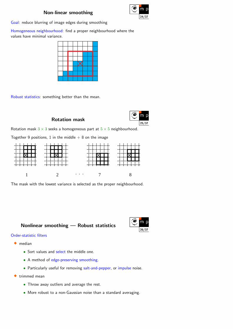
24/37Non-linear smoothing

Goal: reduce blurring of image edges during smoothing

Homogeneous neighbourhood: find a proper neighbourhood where the

values have minimal variance.

Robust statistics: something better than the mean.

25/37Rotation mask

Rotation mask 3× 3 seeks a homogeneous part at 5× 5 neighbourhood.

Together 9 positions, 1 in the middle + 8 on the image

1 2 7 8. . .

The mask with the lowest variance is selected as the proper neighbourhood.

26/37Nonlinear smoothing — Robust statistics

Order-statistic filters

� median

• Sort values and select the middle one.

• A method of edge-preserving smoothing.

• Particularly useful for removing salt-and-pepper, or impulse noise.

� trimmed mean

• Throw away outliers and average the rest.

• More robust to a non-Gaussian noise than a standard averaging.

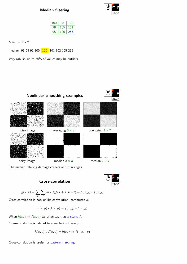
27/37Median filtering

100 98 102

99 105 101

95 100 255

Mean = 117.2

median: 95 98 99 100 100 101 102 105 255

Very robust, up to 50% of values may be outliers.

28/37Nonlinear smoothing examples

noisy image averaging 3× 3 averaging 7× 7

noisy image median 3× 3 median 7× 7

The median filtering damage corners and thin edges.

29/37Cross-correlation

g(x, y) =∑

k

∑l

h(k, l)f(x + k, y + l) = h(x, y) ? f(x, y)

Cross-correlation is not, unlike convolution, commutative

h(x, y) ? f(x, y) 6= f(x, y) ? h(x, y)

When h(x, y) ? f(x, y) we often say that h scans f .

Cross-correlation is related to convolution through

h(x, y) ? f(x, y) = h(x, y) ∗ f(−x,−y)

Cross-correlation is useful for pattern matching

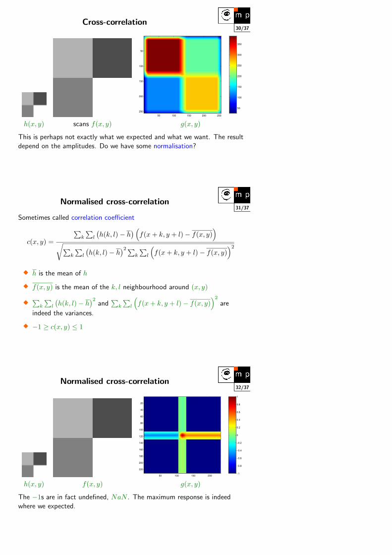
30/37Cross-correlation

50 100 150 200 250

50

100

150

200

25050

100

150

200

250

300

350

h(x, y) scans f(x, y) g(x, y)

This is perhaps not exactly what we expected and what we want. The result

depend on the amplitudes. Do we have some normalisation?

31/37Normalised cross-correlation

Sometimes called correlation coefficient

c(x, y) =

∑k

∑l

(h(k, l)− h

) (f(x + k, y + l)− f(x, y)

)√∑

k

∑l

(h(k, l)− h

)2 ∑k

∑l

(f(x + k, y + l)− f(x, y)

)2

� h is the mean of h

� f(x, y) is the mean of the k, l neighbourhood around (x, y)

�∑

k

∑l

(h(k, l)− h

)2and

∑k

∑l

(f(x + k, y + l)− f(x, y)

)2

are

indeed the variances.

� −1 ≥ c(x, y) ≤ 1

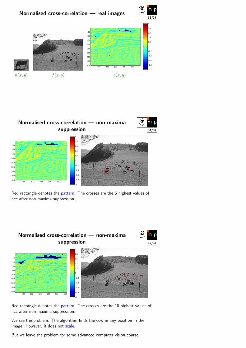
32/37Normalised cross-correlation

50 100 150 200

20

40

60

80

100

120

140

160

180

200

220

−1

−0.8

−0.6

−0.4

−0.2

0

0.2

0.4

0.6

0.8

1

h(x, y) f(x, y) g(x, y)

The −1s are in fact undefined, NaN . The maximum response is indeed

where we expected.

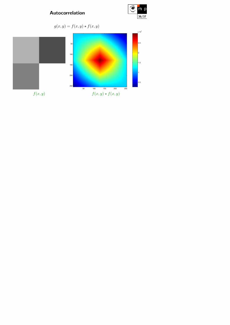
33/37Normalised cross-correlation — real images

100 200 300 400 500

50

100

150

200

250

300

350

400

450

−1

−0.8

−0.6

−0.4

−0.2

0

0.2

0.4

0.6

0.8

1

h(x, y) f(x, y) g(x, y)

34/37

Normalised cross-correlation — non-maximasuppression

100 200 300 400 500

50

100

150

200

250

300

350

400

450

−1

−0.8

−0.6

−0.4

−0.2

0

0.2

0.4

0.6

0.8

1

Red rectangle denotes the pattern. The crosses are the 5 highest values of

ncc after non-maxima suppression.

35/37

Normalised cross-correlation — non-maximasuppression

100 200 300 400 500 600

50

100

150

200

250

300

350

400

450

−1

−0.8

−0.6

−0.4

−0.2

0

0.2

0.4

0.6

0.8

1

Red rectangle denotes the pattern. The crosses are the 10 highest values of

ncc after non-maxima suppression.

We see the problem. The algorithm finds the cow in any position in the

image. However, it does not scale.

But we leave the problem for some advanced computer vision course.

36/37Autocorrelation

g(x, y) = f(x, y) ? f(x, y)

50 100 150 200 250

50

100

150

200

250

0.5

1

1.5

2

2.5

x 104

f(x, y) f(x, y) ? f(x, y)