11

IMAGE PROCESSINGIMAGE PROCESSING

Sonia TangaroSonia TangaroIstituto Nazionale di Fisica NucleareIstituto Nazionale di Fisica Nucleare

Sonia.Tangaro@ba.infn.itSonia.Tangaro@ba.infn.it

22

Programma del CorsoProgramma del Corso

1.1. IntroductionIntroduction2.2. ComponentiComponenti di un di un SistemaSistema di Image Processingdi Image Processing3.3. Digital Image FundamentalsDigital Image Fundamentals

1.1. Basic ConceptsBasic Concepts2.2. Spatial and GraySpatial and Gray--Level ResolutionLevel Resolution3.3. Some basic Relationships between PixelsSome basic Relationships between Pixels

4.4. Image Enhancement in the Spatial Domain Image Enhancement in the Spatial Domain 1.1. Basic Gray Level TransformationsBasic Gray Level Transformations2.2. Histogram ProcessingHistogram Processing3.3. FilteringFiltering

5.5. Image Enhancement in the Frequency Domain Image Enhancement in the Frequency Domain 6.6. SegmentationSegmentation7.7. Pattern recognitionPattern recognition8.8. Classification SystemsClassification Systems

1.1. RegressioneRegressione LogisticaLogistica2.2. RetiReti NeuraliNeurali ArtificialiArtificiali

9.9. Valutazione della qualitValutazione della qualitàà dei Modellidei Modelli

33

Libri di testo ConsigliatiLibri di testo Consigliati

Giudici Giudici -- Data Data MiningMining -- McMc GrawGraw HillHillBishopBishop -- StatisticalStatistical Pattern Pattern RecognitionRecognition -- YYYYYYGonzalesGonzales & & WoodsWoods -- DigitalDigital ImageImage Processing Processing -- PrencticePrenctice HallHall

44

Un processo complessoUn processo complesso

55

Descrizione

In ingresso al sistema di riconoscimento èpresentata una descrizione, cioè un insieme di misure (features) che caratterizza l’oggetto da riconoscere.L’insieme di misure èscelto sulla base delle esigenze specifiche

66

RepresentingRepresenting DigitalDigital ImageImage

The results of sampling and quantization is a matrix of real number.

f (x,y) =

f (0,0) f (0,1)... f (0,N −1)f (1,0) f (1,1)... f (1,N −1)...f (M −1,0) f (M −1,1)... f (M −1,N −1)

⎡

⎣

⎢ ⎢ ⎢ ⎢ ⎢ ⎢ ⎢ ⎢ ⎢

⎤

⎦

⎥ ⎥ ⎥ ⎥ ⎥ ⎥ ⎥ ⎥ ⎥

pixel

image

77

f (x,y) =

f (0,0) f (0,1)... f (0,N −1)f (1,0) f (1,1)... f (1,N −1)...f (M −1,0) f (M −1,1)... f (M −1,N −1)

⎡

⎣

⎢ ⎢ ⎢ ⎢ ⎢ ⎢ ⎢ ⎢ ⎢

⎤

⎦

⎥ ⎥ ⎥ ⎥ ⎥ ⎥ ⎥ ⎥ ⎥

pixel

Y

X

Origin

(x,y)

88

SpatialSpatial and and GrayGray--LevelLevel ResolutionResolution

Sampling is the principal factor determining the spatial resolution of an image.Basically,spatial resolution is the smallest discernible detail in an image.Suppose that we construct a chart with vertical lines of width W,with the space between the lines also having width W.A line pair consists of one such line and its adjacent space. Thus,the width of a line pair is 2W, and there are 1/2W line pairs per unit distance. A widely used definition of resolution is simply the smallest number of discernible line pairs per unit distance; for example,100 line pairs per millimeter.

Gray-level resolution similarly refers to the smallest discernible change in gray level (measuring discernible changes in gray level is a highly subjective process). Due to hardware considerations,the number of gray levels is usually an integer power of 2. The most common number is 8 bits, with 16 bits being used in some applications where enhancement of specific gray-level ranges is necessary. Sometimes we find systems that can digitize the gray levels of an image with 10 or 12 bits of accuracy,but these are the exception rather than the rule.

99

NeighborsNeighbors of a Pixelof a Pixel

pixel p at coordinates (x,y)

horizontal and vertical 4-neighbors of p = N4(p) = (x+1,y) , (x-1,y) , (x,y+1) , (x,y-1)

diagonal 4-neighbors of p = ND(p) = (x+1,y+1) , (x+1,y-1) , (x-1,y+1) , (x+1,y+1)

N4(p) + ND(p) = N8(p) = 8-neighbors

1010

AdjacencyAdjacency1. Connectivity = two pixels are connected if they are neighbors and if their

gray levels satisfy a specified criterion of similarity (say,if their gray levelsare equal)

2. Adjacency. Let V be the set of gray-level values used to define adjacency.Weconsider three types of adjacency: a. 4-adjacency: Two pixels pand qwith values from Vare 4-adjacent if q

is in the set N4(p). b. 8-adjacency: Two pixels pand qwith values from Vare 8-adjacent if q

is in the set N(p). c. m-adjacency (mixed adjacency): Two pixels pand qwith values from V

are m-adjacent if(i) q is in in N4(p),or (ii) q is in ND(p)andthe set has no pixels whose values are from VMixed adjacency is a modification of 8-adjacency.It is introduced to

eliminate the ambiguities that often arise when 8-adjacency isused.

For example

1111

ConnectivityConnectivity, , RegionsRegions, and , and BoundariesBoundaries

A (digital) path(or curve) from pixel p (x, y) to pixel q (s,t) is a sequence of distinct pixels with coordinates

(x0 , y0), (x1 , y1), … , (xn , yn)where (x0 , y0) =(x, y), (xi-1 , yi-1), (xi , yi) (xn , yn) =(s, t), and pixels and are adjacent for 1< i < n. In this case, n is the length of the path. If (x0 , y0) =(xn , yn), the path is a closed pathLet S represent a subset of pixels in an image.Two pixels p and q are said tobe connected in S if there exists a path between them consisting entirely of pixels in S. For any pixel p in S, the set of pixels that are connected to it in S is called a connected component of S. If it only has one connectedcomponent, then set S is called a connected set.Let R be a subset of pixels in an image. We call R a region of the image if R is a connected set.The boundary (also called border or contour) of a region R is the set of pixelsin the region that have one or more neighbors that are not in R.

1212

EnhancementEnhancement isis toto processprocess anan imageimage so so thatthat the the resultresult isis more more suitablesuitable thanthan the the originaloriginal imageimage forfor a a specificspecific applicationapplication

SpatialSpatial domaindomain = direct = direct manipulationmanipulation of of pixelspixels in in anan imageimage

FrequencyFrequency domaindomain = = modifyingmodifying the the FourierFourier transormtransorm of of ananimageimage

ImageImage EnhancementEnhancement in the in the SpatialSpatialDomainDomain

1313

EnhancementEnhancement techniquestechniques basedbasedon on PointPoint Processing Processing

g(x,y)g(x,y)=T=T[f(x,y)][f(x,y)]s=Ts=T( r )( r )

Contrast stretching:the values of r below m are compressed by the transformation function into a narrow range of s,toward black; the opposite effect takes place for values of rabove m.In the limiting case shown in Fig.(b), T(r)produces a two-level (binary) image.A mapping of this form is called a thresholding function.

1414

EnhancementEnhancement techniquestechniques basedbased on on maskmask processing or processing or filteringfiltering

Y

X

Origin

(x,y)

One of the principal approaches in this formulation is based on the use of so-called masks (also referred to as filters, kernels, templates, or windows). Basically, a mask is a small (say, 3*3) 2-D array,such as the one shown in Fig., in which the values of the mask coefficients determine the nature of the process, such as image sharpening.

(3x3 mask)

1515

GrayGray LevelLevel TransformationsTransformations

1. Image Negatives : s =L-1-r2. Log Transformations : s =c log (1+r)3. Power-Law Transformations : s = c rγ

1616

Image Negatives : s =L-1-r

ThisThis typetype of processing of processing isis particularlyparticularly suitedsuited forfor enhancingenhancing whitewhite or or graygraydetaildetail embeddedembedded in dark in dark regionsregions of of anan imageimage,,eses-- peciallypecially whenwhen the the black black areasareas are are dominantdominant in in sizesize..AnAn exampleexample isis shownshown in in FigFig..The ..The originaloriginal imageimage isis a a digitaldigital mammogrammammogram showingshowing a a smallsmall lesionlesion.In .In spitespiteof the of the factfact thatthat the visual the visual contentcontent isis the the samesame in in bothboth imagesimages, note , note howhowmuchmuch easiereasier itit isis toto analyzeanalyze the the breastbreast tissuetissue in the negative in the negative imageimage in in thisthis particularparticular case.case.

1717

Log Transformations : s =c log (1+r)

(a)(a)FourierFourier spectrumspectrum. . (b)(b)ResultResult of of applyingapplying the log the log transformationtransformation

givengiven in in EqEq. . withwith c=1c=1. .

1818

Power-Law Transformations : s = c rγ

(a)(a)MagneticMagnetic resonanceresonance (MR) (MR) imageimage of a of a fracturedfractured humanhuman spine. spine. (b)(b)��((d)d)ResultsResults of of applyingapplying the the transformationtransformation in in EqEq. . withwith c=1andc=1and γγ==0.6,0.4,and 0.3,0.6,0.4,and 0.3,respectively.respectively.

1919

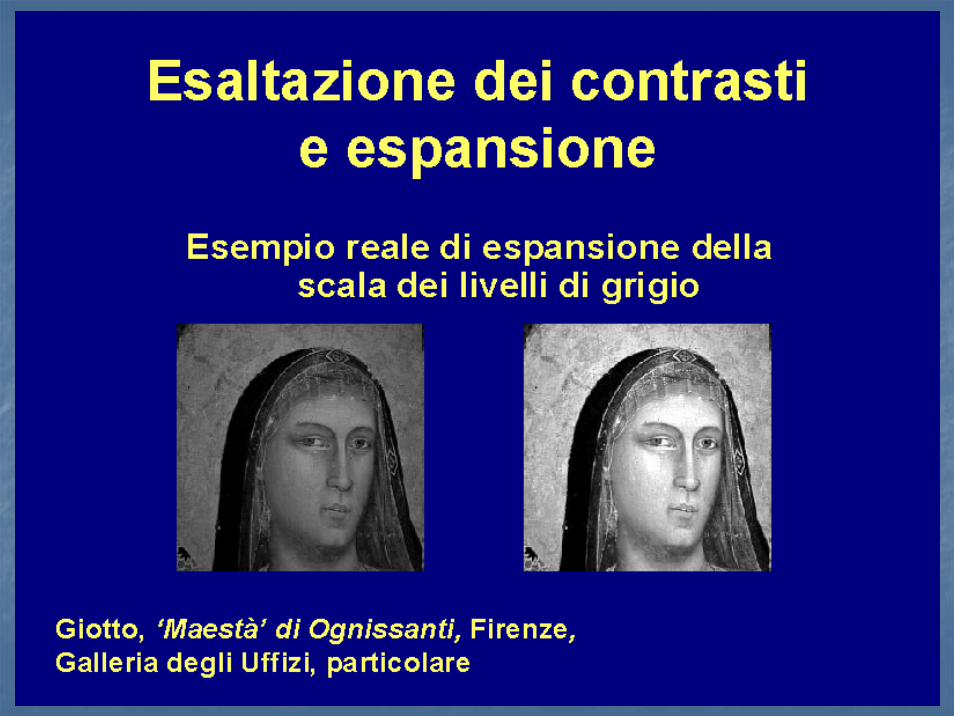
Elaborazioni locali spazialiElaborazioni locali spaziali

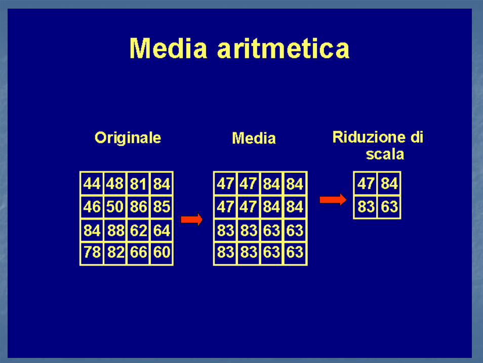
Esaltazione dei contrasti e espansioneEsaltazione dei contrasti e espansioneIstogrammaIstogrammaMedia AritmeticaMedia Aritmetica

2020

2121

2222

2323

2424

2525

2626

2727

2828

2929

3030

3131

3232

3333

3434

3535

3636

3737

3838

3939

Elaborazioni locali spazialiElaborazioni locali spaziali

Esaltazione dei contrasti e espansioneEsaltazione dei contrasti e espansioneIstogrammaIstogrammaMedia AritmeticaMedia Aritmetica

4040

414130

4242

4343

4444

4545

4646

4747

4848

4949

5050

5151

5252

5353

5454

5555

Elaborazioni locali spazialiElaborazioni locali spazialiSommarioSommario

Esaltazione dei contrasti e espansioneEsaltazione dei contrasti e espansioneIstogrammaIstogrammaMedia AritmeticaMedia Aritmetica

5656

5757

5858

5959

6060

6161

6262

6363

6464

6565

6666

6767

6868

6969

7070

717160

7272

FILTRIFILTRI

Possiamo considerare la media aritmetica Possiamo considerare la media aritmetica come un filtro applicato allcome un filtro applicato all’’immagineimmagineSono stati studiati unSono stati studiati un’’infinitinfinitàà di filtri di filtri Esempio: il filtro Esempio: il filtro gaussianogaussiano

7373

7474

7575

GrayGray--level discontinuity detectionlevel discontinuity detection

Basic types of grayBasic types of gray--level discontinuities in a digital image: level discontinuities in a digital image: -- pointspoints-- lineslines-- edgesedges

Main approach for their identification: to run a Main approach for their identification: to run a maskmask through the through the images, computing the sum of products of the coefficients with timages, computing the sum of products of the coefficients with the he gray levels contained in the region encompassed by the mask. gray levels contained in the region encompassed by the mask.

a general 3x3 mask

(*)Response of the mask at any point in the image, defined with respect to its center location.

zi= gray level of the pixel ωi =associated mask coefficient

7676

MASKMASK

In general, linear filtering of animage f of size M*Nwith a filter mask of size m*n isgiven by the expression:

where, from the previousparagraph, a=(m-1)/2 and b=(n-1)/2. To generate a complete filtered image thisequation must be applied forx=0, 1,2, … , M-1 and y=0, 1, 2, … , N-1. In this way, weare assured that the

7777

7878

7979

8080

8181

8282

8383

8484

8585

8686

8787

8888

8989

9090

9191

9292

9393

9494

9595

9696

9797

9898

9999

100100

101101

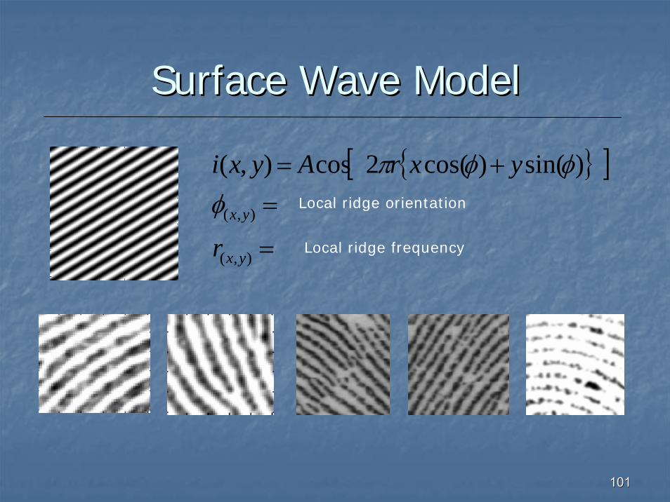
Surface Wave ModelSurface Wave Model

[ { } ]

=

=+=

),(

),(

)sin()cos(2cos),(

yx

yx

r

yxrAyxiφ

φφπLocal ridge orientation

Local ridge frequency

102102

Validity of the modelValidity of the model

With the exception of singularities such as core and delta, any local region of the fingerprint has consistent ridge orientationand frequency. The ridge flow may be coarsely approximated using an oriented surface wave that can be identified using a single frequency f and orientation θ. However, a real fingerprint is marked by a distribution of multiple frequencies and orientation.