Embed Size (px)
Citation preview
Image Processing
Traitement d’images
Silvia Valerosilvia.valerosilvia.valero--valbuena@[email protected]
http://www.gipsahttp://www.gipsa--lab.inpg.fr/~silvia.valerolab.inpg.fr/~silvia.valero--valbuena/valbuena/

Image Processing
Outline
• Introduction: Digital images• Histogram modification• Noise reduction• Edge detection• 2D Fourier Transform• Bases of mathematical morphology• Examples of image processing
Image Processing
Bibliography
• Digital Image Processing, 2nd Edition by Gonzalez and Woods Prentice Hall, 2002
• Digital Image Processing Using MATLABby Gonzalez, Woods, and Eddins, PrenticeHall, 2004
• Analyse d'images : Filtrage et segmentationBy Cocquerez and Philipp, Masson, 1995
• Traitement et analyse des images num ériquesBy Bres, Jolion and Lebourgeois, Herm ès, 2003

Introduction:Digital images
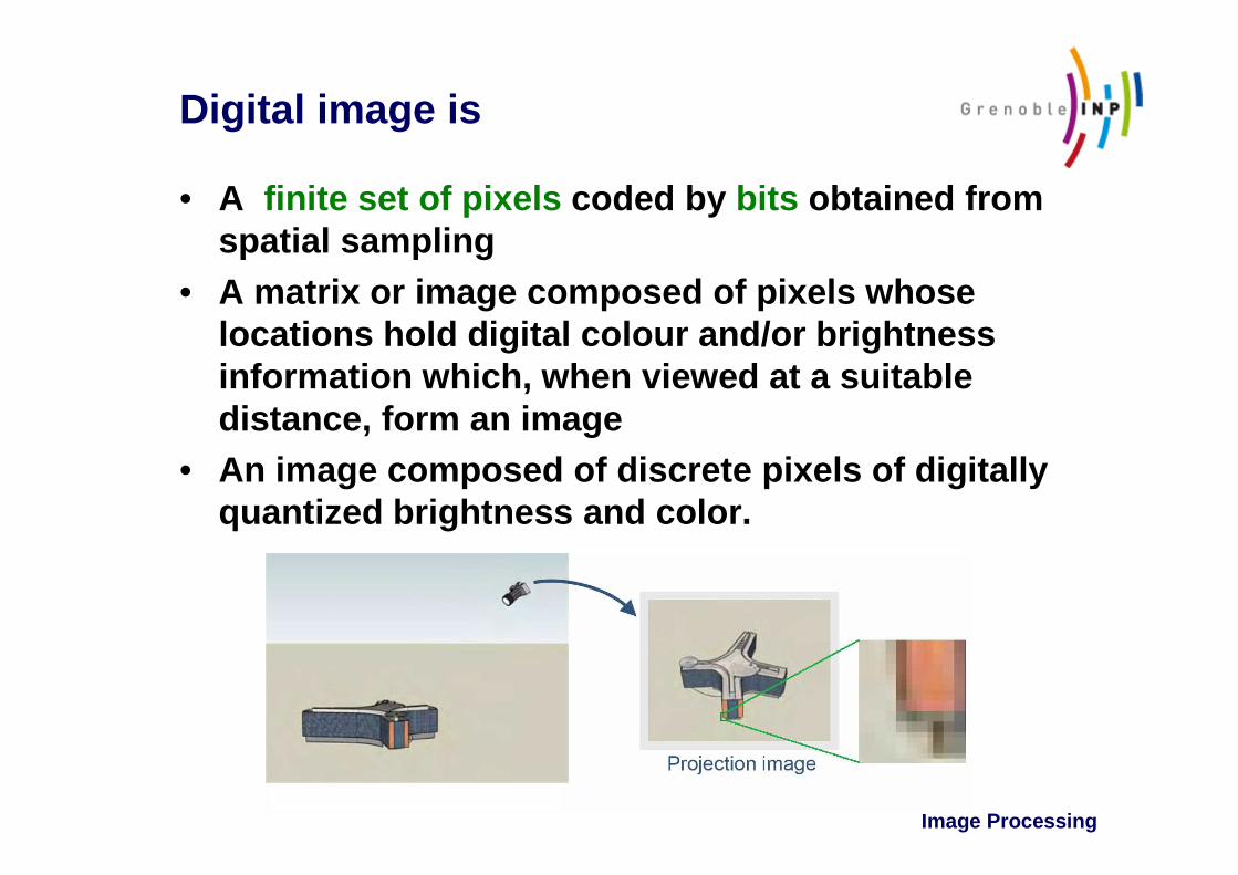
Image Processing
Digital image is
• A finite set of pixels coded by bits obtained from spatial sampling
• A matrix or image composed of pixels whose locations hold digital colour and/or brightness information which, when viewed at a suitable distance, form an image
• An image composed of discrete pixels of digitally quantized brightness and color.
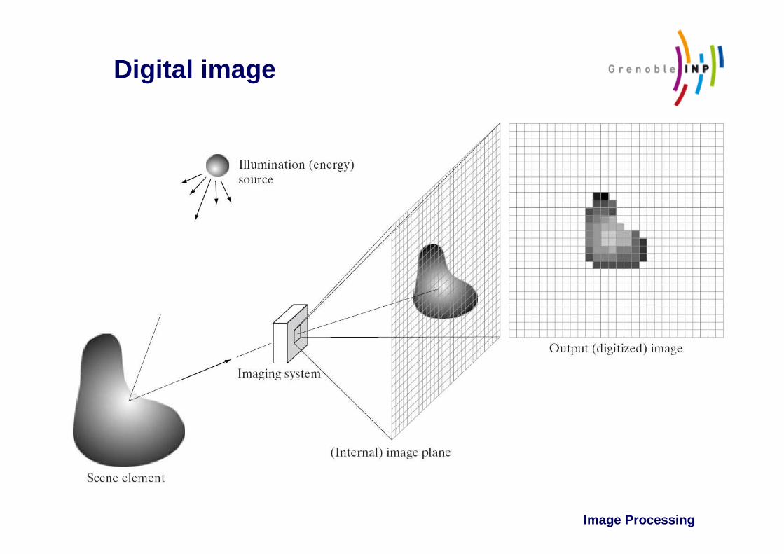
Image Processing
Digital image
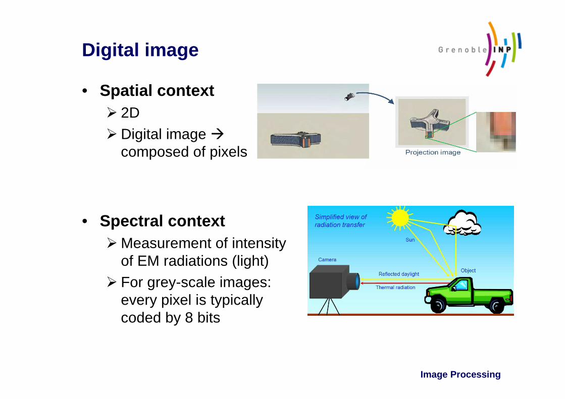
Image Processing
Digital image
• Spatial context� 2D
� Digital image �composed of pixels
• Spectral context� Measurement of intensity
of EM radiations (light)
� For grey-scale images:every pixel is typicallycoded by 8 bits
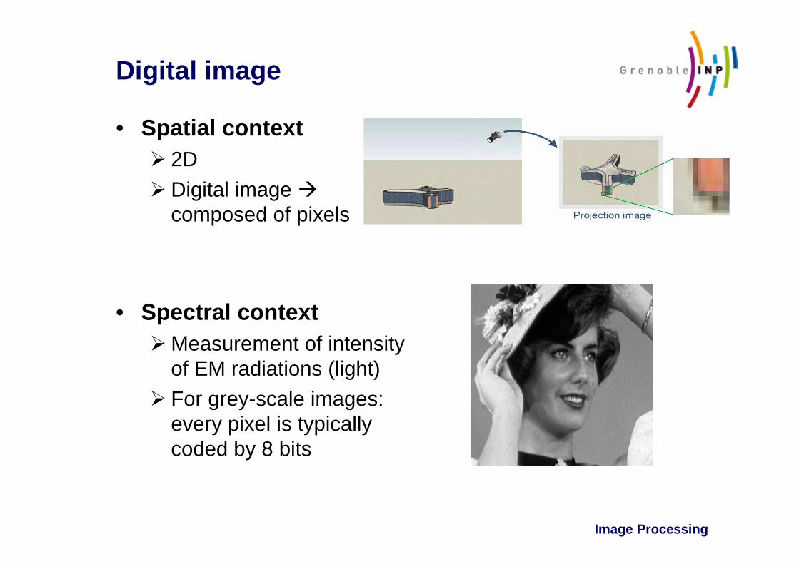
Image Processing
Digital image
• Spatial context� 2D
� Digital image �composed of pixels
• Spectral context� Measurement of intensity
of EM radiations (light)
� For grey-scale images:every pixel is typicallycoded by 8 bits

Image Processing
Digital image
• Spatial context� 2D
� Digital image �composed of pixels
• Spectral context� For grey-scale images:
every pixel is typicallycoded by 8 bits
� For color images:every pixel has 3 components:red, green, blue,each of them coded by 8 bits

Image Processing
Grey levels and look-up table
• Every value of the pixelis associated with one coloraccording to the color look-up table
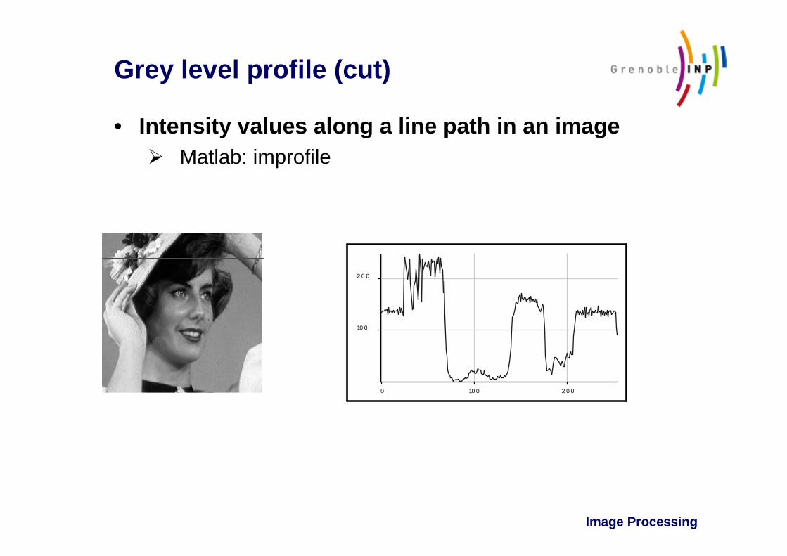
Image Processing
Grey level profile (cut)
• Intensity values along a line path in an image� Matlab: improfile
0 10 0 2 0 0
10 0
2 0 0

Image Processing
Image sampling and quantization
• Sampling meansdigitizing thecoordinatevalues
• Quantizationmeansdigitizingthe amplitudevalues
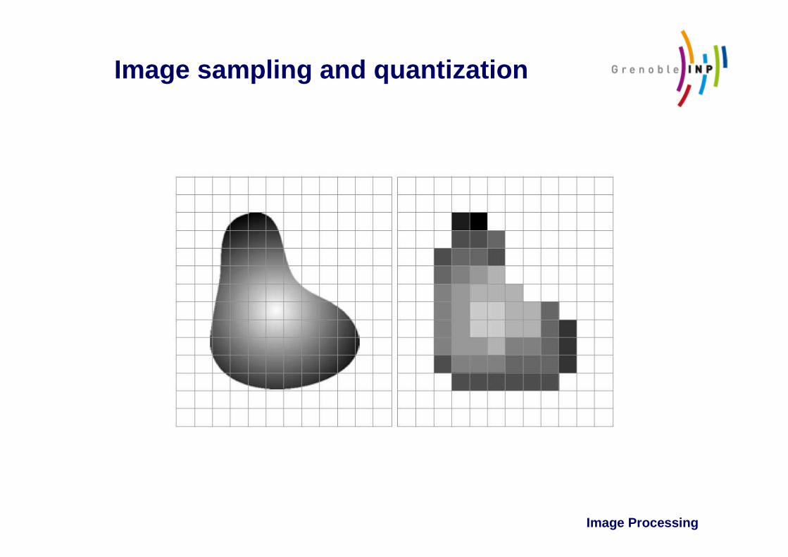
Image Processing
Image sampling and quantization

Image Processing
Quantization
Muscle cells:
4 bits 2 bits
8 bits 3 bits
Face:

Image Processing
Sampling
• Sampling is the principal factor determining the spatial resolution of an image
• Not relevant sampling can result in image pixelization
Pixelization is primarily used for censorship
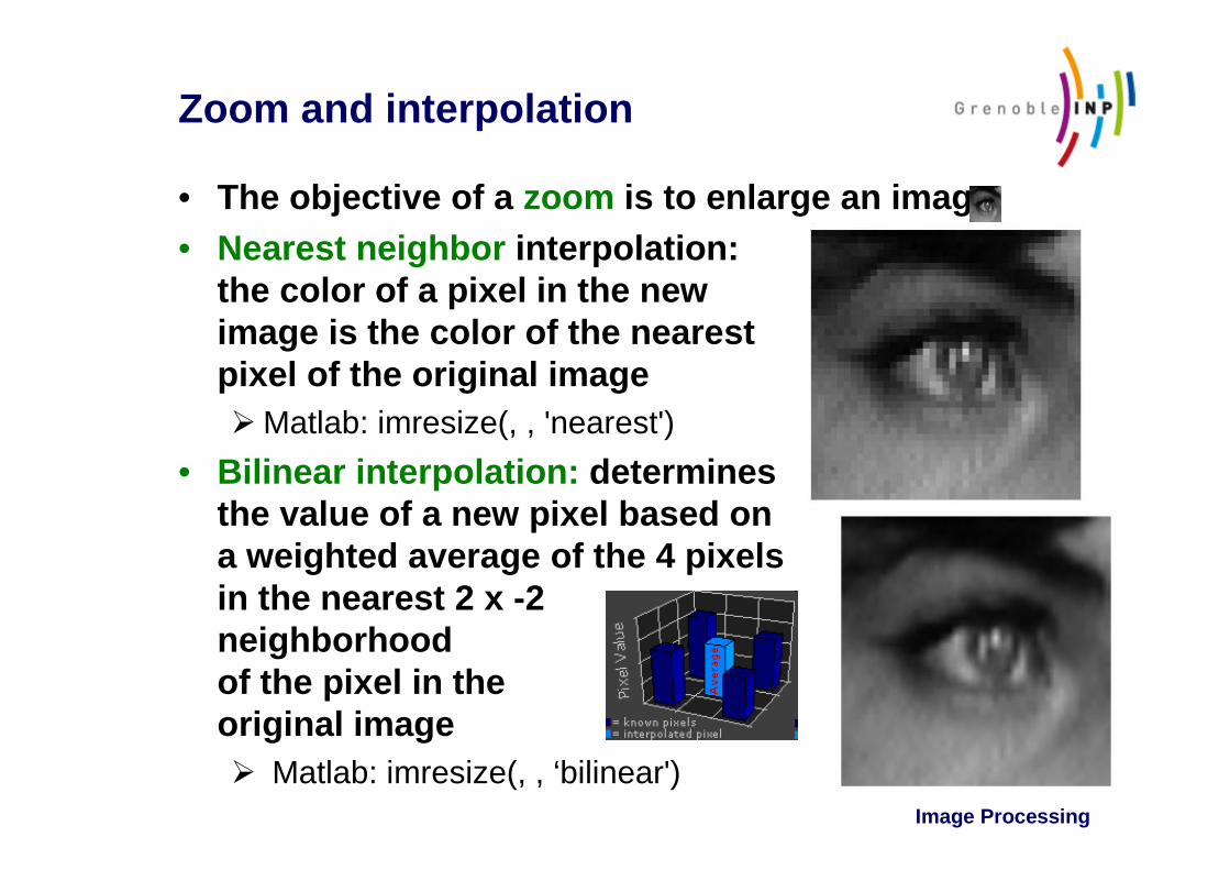
Image Processing
Zoom and interpolation
• The objective of a zoom is to enlarge an image• Nearest neighbor interpolation:
the color of a pixel in the newimage is the color of the nearestpixel of the original image� Matlab: imresize(, , 'nearest')
• Bilinear interpolation: determinesthe value of a new pixel based ona weighted average of the 4 pixelsin the nearest 2 x -2neighborhoodof the pixel in theoriginal image � Matlab: imresize(, , ‘bilinear')

Image Processing
Aliasing
• If the image is undersampled (Shannon sampling theorem requires Fe < 2 Fmax), aliasing corrupts the sampled image
• New frequency components can appear• To avoid aliasing: low -pass filtering prior to sampling
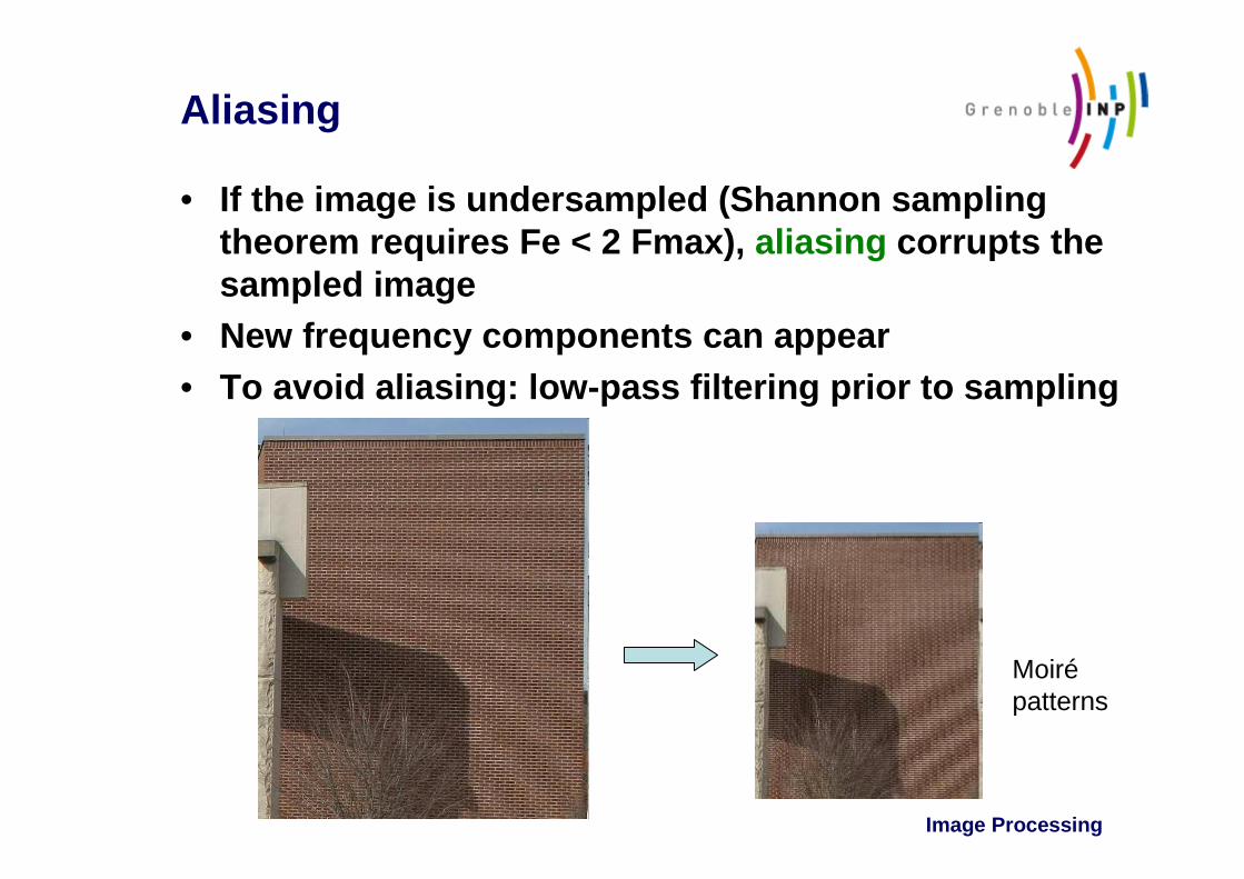
Image Processing
Aliasing
• If the image is undersampled (Shannon sampling theorem requires Fe < 2 Fmax), aliasing corrupts the sampled image
• New frequency components can appear• To avoid aliasing: low -pass filtering prior to sampling
Moirépatterns

Image Processing
Measuring the difference between images
• To measure image degradation, a new image can be compared with the original image (using Hamming distance)
• Mean Absolute Error:
• Mean Square Error:
• Signal to Noise Ratio (dB):
• Peak Signal to Noise Ratio:
( ) ( )∑∑= =
−⋅=M
m
N
n
nmfnmfNM
MAE1 1
,~
,1
( ) ( )( )∑∑= =
−⋅=M
m
N
n
nmfnmfNM
MSE1 1
2,
~,1
( )
( ) ( )( )
−⋅
⋅⋅=
∑∑
∑∑
= =
= =M
m
N
n
M
m
N
n
nmfnmfNM
nmfNM
SNR
1 1
2
1 1
2
,~
,1
,1
log10
( ) ( )( )
−⋅⋅
⋅=∑∑
= =
M
m
N
n
nmfnmfNM
PSNR
1 1
2
2
,~
,1
255log10
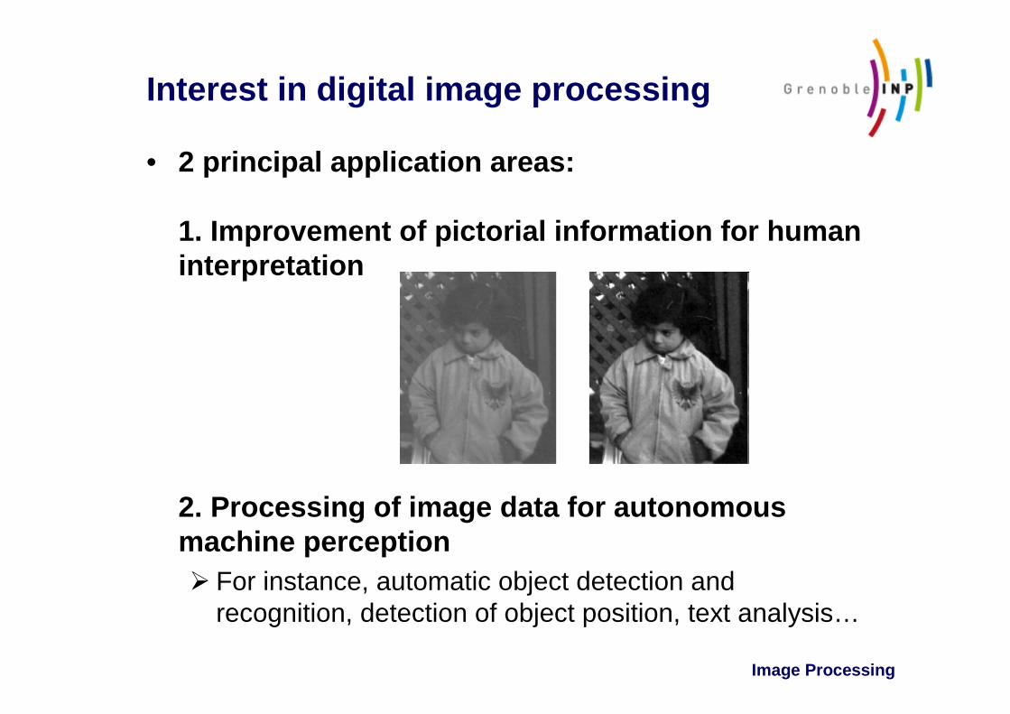
Image Processing
Interest in digital image processing
• 2 principal application areas:
1. Improvement of pictorial information for human interpretation
2. Processing of image data for autonomousmachine perception� For instance, automatic object detection and
recognition, detection of object position, text analysis…

Histogram modification

Image Processing
Image enhancement
• The objective: to process an image so that the result is more suitable than the original image for a specific application
• Image enhancement� In the spatial domain: based on direct manipulation of
pixels in an image
� In the frequency domain: modifying the Fourier transform of an image

Image Processing
Histogram modification
• Grey level transform: Neighborhood is of size 1x1• Image negative: v(x,y) =255 – v(x,y)
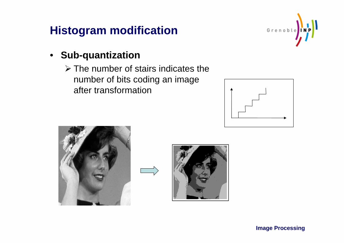
Image Processing
Histogram modification
• Sub-quantization� The number of stairs indicates the
number of bits coding an imageafter transformation

Image Processing
Histogram modification
• Thresholding� A particular case of sub-quantization
t
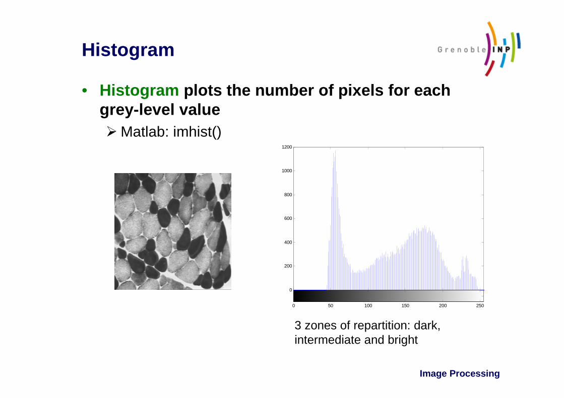
Image Processing
Histogram
• Histogram plots the number of pixels for each grey-level value� Matlab: imhist()
0 50 100 150 200 250
0
200
400
600
800
1000
1200
3 zones of repartition: dark, intermediate and bright
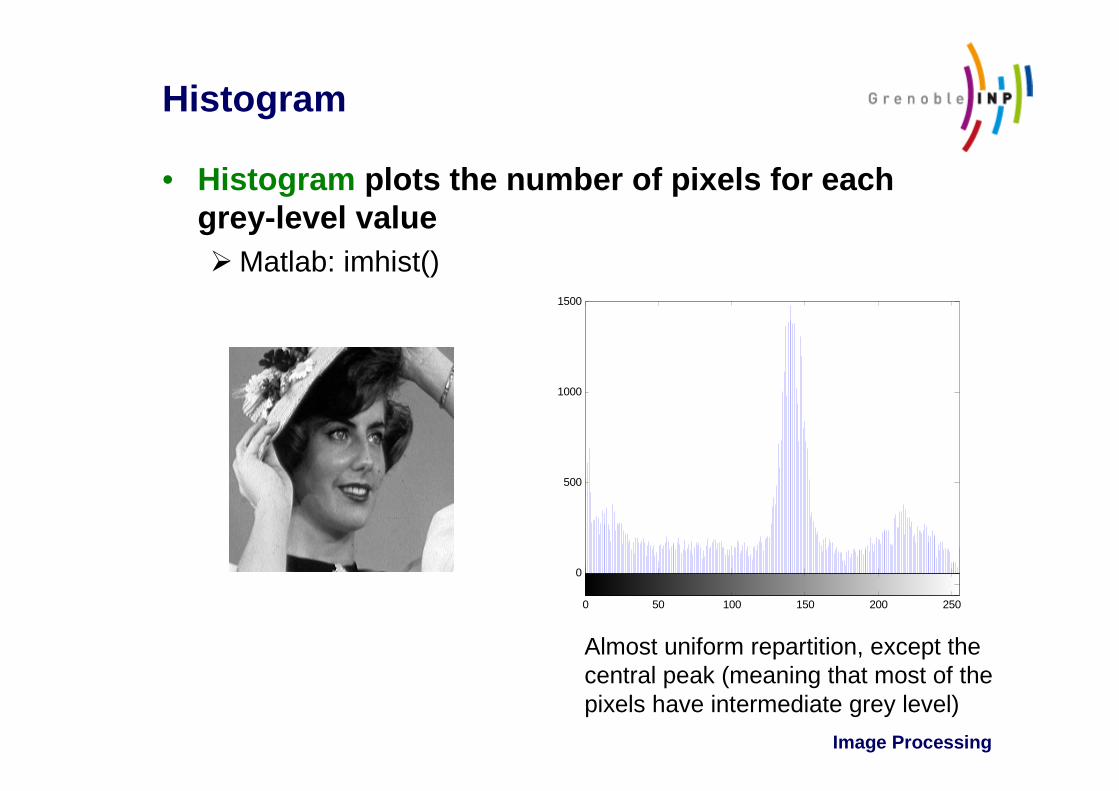
Image Processing
Histogram
• Histogram plots the number of pixels for each grey-level value� Matlab: imhist()
Almost uniform repartition, except the central peak (meaning that most of the pixels have intermediate grey level)
0 50 100 150 200 250
0
500
1000
1500
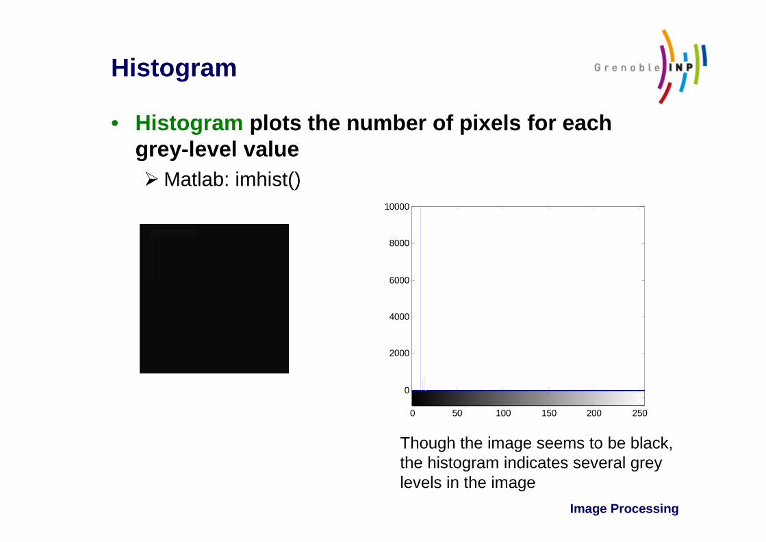
Image Processing
Histogram
• Histogram plots the number of pixels for each grey-level value� Matlab: imhist()
Though the image seems to be black, the histogram indicates several grey levels in the image
0 50 100 150 200 250
0
2000
4000
6000
8000
10000

Image Processing
Histograms are the basis for numerous spatial processing techniques
� Image enhancement
� Segmentation
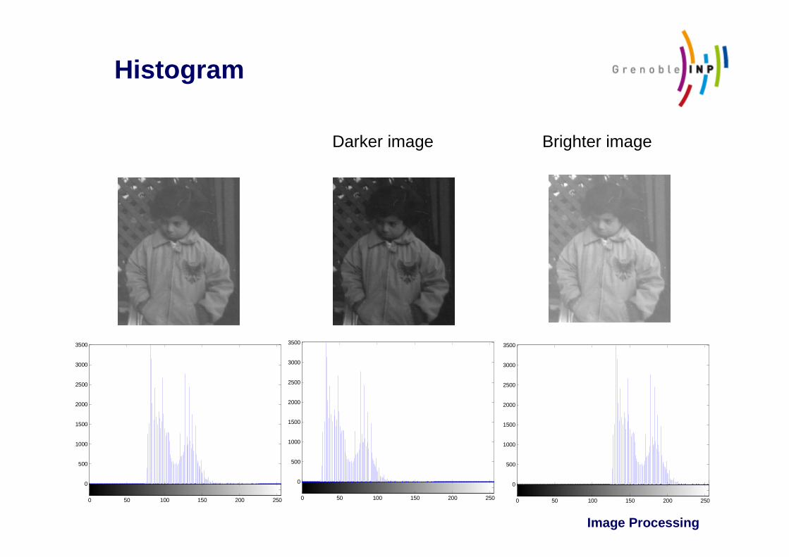
Image Processing
Histogram
0 50 100 150 200 250
0
500
1000
1500
2000
2500
3000
3500
0 50 100 150 200 250
0
500
1000
1500
2000
2500
3000
3500
Darker image
0 50 100 150 200 250
0
500
1000
1500
2000
2500
3000
3500
Brighter image

Image Processing
Histogram: Linear rescaling of the range
• The distance between peaks is constant
0 50 100 150 200 250
0
500
1000
1500
2000
2500
3000
3500
4000
4500
5000
?

Image Processing
Histogram: Linear rescaling of the range
• The distance between peaks is constant
0 50 100 150 200 250
0
500
1000
1500
2000
2500
3000
3500
4000
4500
5000
0 50 100 150 200 250
0
500
1000
1500
2000
2500
3000
3500
4000
4500
5000
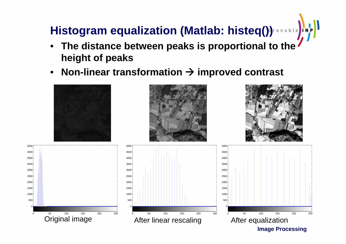
Image Processing
Histogram equalization (Matlab: histeq())• The distance between peaks is proportional to the
height of peaks• Non-linear transformation ���� improved contrast
0 50 100 150 200 250
0
500
1000
1500
2000
2500
3000
3500
4000
4500
5000
0 50 100 150 200 250
0
500
1000
1500
2000
2500
3000
3500
4000
4500
5000
0 50 100 150 200 250
0
500
1000
1500
2000
2500
3000
3500
4000
4500
5000
Original image After linear rescaling After equalization