Embed Size (px)
Citation preview

Image Processing Toolbox™
Provide feedback about this page
Example 1 — Reading and Writing Images
On this page…
Introduction
Step 1: Read and Display an Image
Step 2: Check How the Image Appears in the Workspace
Step 3: Improve Image Contrast
Step 4: Write the Image to a Disk File
Step 5: Check the Contents of the Newly Written File
Introduction
This example introduces some basic image processing concepts. The example starts by reading an image into the MATLAB workspace. The example then performs some contrast adjustment on the image. Finally, the example writes the adjusted image to a file.
Back to Top
Step 1: Read and Display an Image
First, clear the MATLAB workspace of any variables and close open figure windows.
close all
To read an image, use the imread command. The example reads one of the sample images included with the toolbox, pout.tif, and stores it in an array named I.
I = imread('pout.tif');
imread infers from the file that the graphics file format is Tagged Image File Format (TIFF). For the list of supported graphics file formats, see the imread function reference documentation.

Now display the image. The toolbox includes two image display functions: imshow and imtool. imshow is the toolbox's fundamental image display function. imtool starts the Image Tool which presents an integrated environment for displaying images and performing some common image processing tasks. The Image Tool provides all the image display capabilities of imshow but also provides access to several other tools for navigating and exploring images, such as scroll bars, the Pixel Region tool, Image Information tool, and the Contrast Adjustment tool. For more information, see Displaying and Exploring Images. You can use either function to display an image. This example uses imshow.
imshow(I)
Grayscale Image pout.tif
Back to Top
Step 2: Check How the Image Appears in the Workspace
To see how the imread function stores the image data in the workspace, check the Workspace browser in the MATLAB desktop. The Workspace browser displays information about all the variables you create during a MATLAB session. The imread function returned the image data in the variable I, which is a 291-by-240 element array of uint8 data. MATLAB can store images as uint8, uint16, or doublearrays.
You can also get information about variables in the workspace by calling the whos command.
whos
MATLAB responds with

Name Size Bytes Class Attributes
I 291x240 69840 uint8
For more information about image storage classes, see Converting Between Image Classes.
Back to Top
Step 3: Improve Image Contrast
pout.tif is a somewhat low contrast image. To see the distribution of intensities in pout.tif, you can create a histogram by calling theimhist function. (Precede the call to imhist with the figure command so that the histogram does not overwrite the display of the image Iin the current figure window.)
figure, imhist(I)
Notice how the intensity range is rather narrow. It does not cover the potential range of [0, 255], and is missing the high and low values that would result in good contrast.
The toolbox provides several ways to improve the contrast in an image. One way is to call the histeq function to spread the intensity values over the full range of the image, a process called histogram equalization.
I2 = histeq(I);
Display the new equalized image, I2, in a new figure window.
figure, imshow(I2)

Equalized Version of pout.tif
Call imhist again to create a histogram of the equalized image I2. If you compare the two histograms, the histogram of I2 is more spread out than the histogram of I1.
figure, imhist(I2)
The toolbox includes several other functions that perform contrast adjustment, including the imadjust and adapthisteq functions. SeeAdjusting Pixel Intensity Values for more information. In addition, the toolbox includes an interactive tool, called the Adjust Contrast tool, that you can use to adjust the contrast and brightness of an image displayed in the Image Tool. To use this tool, call the imcontrastfunction or access the tool from the Image Tool. For more information, see Adjusting Image Contrast Using the Adjust Contrast Tool.

Back to Top
Step 4: Write the Image to a Disk File
To write the newly adjusted image I2 to a disk file, use the imwrite function. If you include the filename extension '.png', the imwritefunction writes the image to a file in Portable Network Graphics (PNG) format, but you can specify other formats.
imwrite (I2, 'pout2.png');
See the imwrite function reference page for a list of file formats it supports. See also Writing Image Data to a File for more information about writing image data to files.
Back to Top
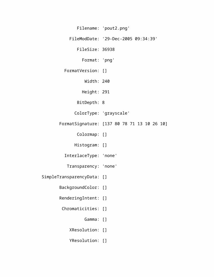
Step 5: Check the Contents of the Newly Written File
To see what imwrite wrote to the disk file, use the imfinfo function.
imfinfo('pout2.png')
The imfinfo function returns information about the image in the file, such as its format, size, width, and height. See Getting Information About a Graphics File for more information about using imfinfo.
ans =
Filename: 'pout2.png'
FileModDate: '29-Dec-2005 09:34:39'
FileSize: 36938
Format: 'png'
FormatVersion: []
Width: 240
Height: 291
BitDepth: 8
ColorType: 'grayscale'
FormatSignature: [137 80 78 71 13 10 26 10]
Colormap: []
Histogram: []
InterlaceType: 'none'
Transparency: 'none'
SimpleTransparencyData: []
BackgroundColor: []
RenderingIntent: []
Chromaticities: []
Gamma: []
XResolution: []
YResolution: []
ResolutionUnit: []
XOffset: []
YOffset: []
OffsetUnit: []
SignificantBits: []
ImageModTime: '29 Dec 2005 14:34:39 +0000'
Title: []
Author: []
Description: []
Copyright: []
CreationTime: []
Software: []
Disclaimer: []
Warning: []
Source: []
Comment: []
OtherText: []
Back to Top
Provide feedback about this page
Product Overview Example 2 — Analyzing Images
© 1984-2009- The MathWorks, Inc. - Site Help - Patents - Trademarks - Privacy Policy - Preventing Piracy - RSS
Image Processing Toolbox™
Provide feedback about this page
Example 2 — Analyzing Images
On this page…
Introduction
Step 1: Read Image
Step 2: Use Morphological Opening to Estimate the Background
Step 3: View the Background Approximation as a Surface
Step 4: Subtract the Background Image from the Original Image

Step 5: Increase the Image Contrast
Step 6: Threshold the Image
Step 7: Identify Objects in the Image
Step 8: Examine One Object
Step 9: View All Objects
Step 10: Compute Area of Each Object
Step 11: Compute Area-based Statistics
Step 12: Create Histogram of the Area
Introduction
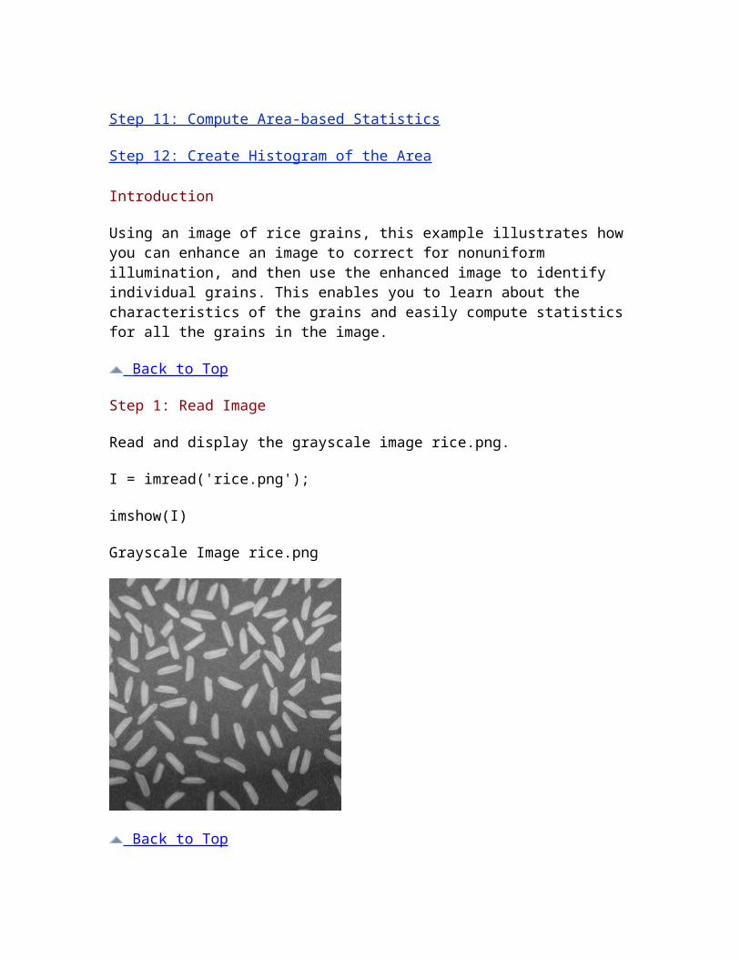
Using an image of rice grains, this example illustrates how you can enhance an image to correct for nonuniform illumination, and then use the enhanced image to identify individual grains. This enables you to learn about the characteristics of the grains and easily compute statistics for all the grains in the image.
Back to Top
Step 1: Read Image
Read and display the grayscale image rice.png.
I = imread('rice.png');
imshow(I)
Grayscale Image rice.png

Back to Top
Step 2: Use Morphological Opening to Estimate the Background
In the sample image, the background illumination is brighter in the center of the image than at the bottom. In this step, the example uses a morphological opening operation to estimate the background illumination. Morphological opening is an erosion followed by a dilation, using the same structuring element for both operations. The opening operation has the effect of removing objects that cannot completely contain the structuring element. For more information about morphological image processing, see Morphological Operations.
background = imopen(I,strel('disk',15));
The example calls the imopen function to perform the morphological opening operation. Note how the example calls the strel function to create a disk-shaped structuring element with a radius of 15. To remove the rice grains from the image, the structuring element must be sized so that it cannot fit entirely inside a single grain of rice.
Back to Top
Step 3: View the Background Approximation as a Surface
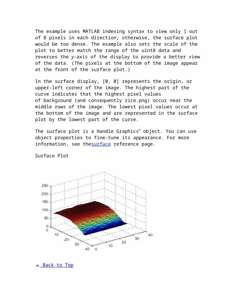
Use the surf command to create a surface display of the background (the background approximation created in Step 2). The surfcommand creates colored parametric surfaces that enable you to view mathematical functions over a rectangular region. However, thesurf function requires data of class double, so you first need to convert background using the double command:
figure, surf(double(background(1:8:end,1:8:end))),zlim([0 255]);
set(gca,'ydir','reverse');
The example uses MATLAB indexing syntax to view only 1 out of 8 pixels in each direction; otherwise, the surface plot would be too dense. The example also sets the scale of the plot to better match the range of the uint8 data and reverses the y-axis of the display to provide a better view of the data. (The pixels at the bottom of the image appear at the front of the surface plot.)
In the surface display, [0, 0] represents the origin, or upper-left corner of the image. The highest part of the curve indicates that the highest pixel values of background (and consequently rice.png) occur near the middle rows of the image. The lowest pixel values occur at the bottom of the image and are represented in the surface plot by the lowest part of the curve.
The surface plot is a Handle Graphics® object. You can use object properties to fine-tune its appearance. For more information, see thesurface reference page.
Surface Plot
Back to Top
Step 4: Subtract the Background Image from the Original Image
To create a more uniform background, subtract the background image, background, from the original image, I, and then view the image:
I2 = I - background;

imshow(I2)
Image with Uniform Background
Back to Top
Step 5: Increase the Image Contrast
After subtraction, the image has a uniform background but is now a bit too dark. Use imadjust to adjust the contrast of the image.imadjust increases the contrast of the image by saturating 1% of the data at both low and high intensities of I2 and by stretching the intensity values to fill the uint8 dynamic range. See the imadjust reference page for more information.
The following example adjusts the contrast in the image created in the previous step and displays it:
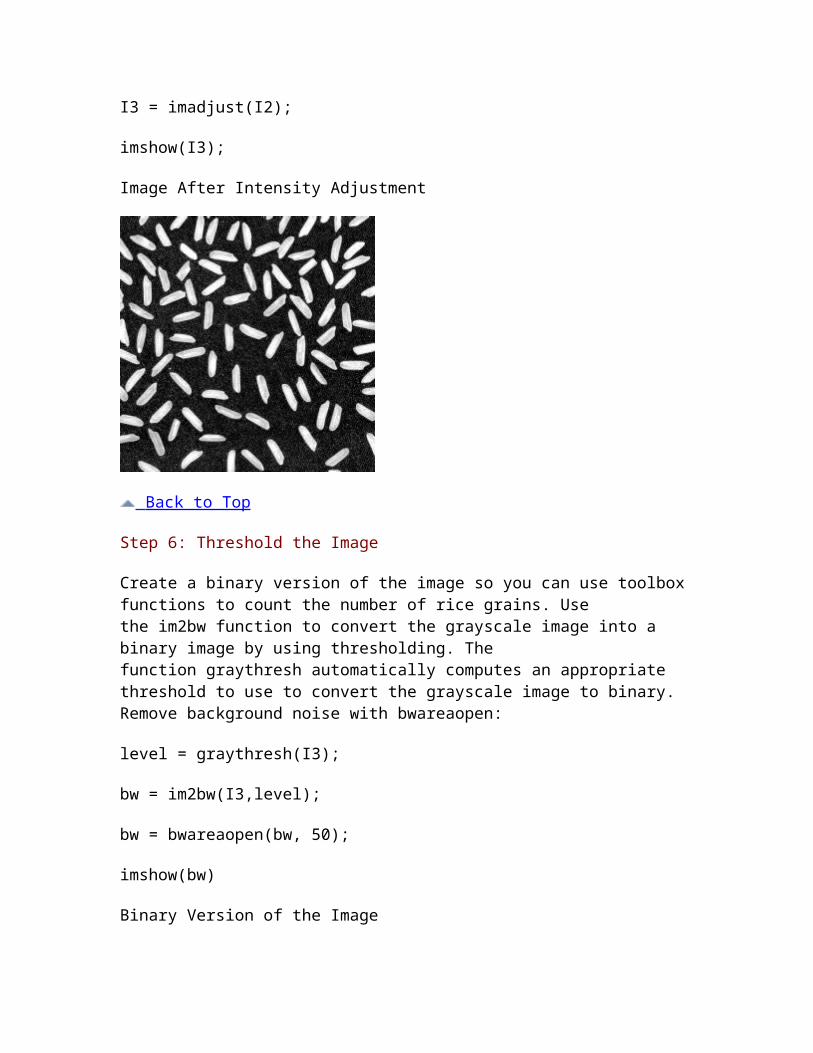
I3 = imadjust(I2);
imshow(I3);
Image After Intensity Adjustment
Back to Top
Step 6: Threshold the Image
Create a binary version of the image so you can use toolbox functions to count the number of rice grains. Use the im2bw function to convert the grayscale image into a binary image by using thresholding. The function graythresh automatically computes an appropriate threshold to use to convert the grayscale image to binary. Remove background noise with bwareaopen:
level = graythresh(I3);
bw = im2bw(I3,level);
bw = bwareaopen(bw, 50);
imshow(bw)
Binary Version of the Image

Back to Top
Step 7: Identify Objects in the Image
The function bwconncomp finds all the connected components (objects) in the binary image. The accuracy of your results depends on the size of the objects, the connectivity parameter (4, 8, or arbitrary), and whether or not any objects are touching (in which case they could be labeled as one object). Some of the rice grains in bw are touching.
cc = bwconncomp(bw, 4);
cc.NumObjectscc =
Connectivity: 4
ImageSize: [256 256]
NumObjects: 95
PixelIdxList: {1x95 cell}
ans =
95
Back to Top
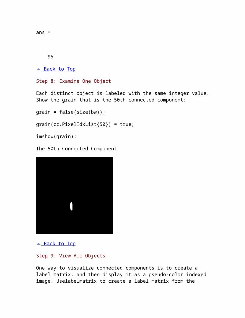
Step 8: Examine One Object
Each distinct object is labeled with the same integer value. Show the grain that is the 50th connected component:
grain = false(size(bw));
grain(cc.PixelIdxList{50}) = true;
imshow(grain);
The 50th Connected Component
Back to Top
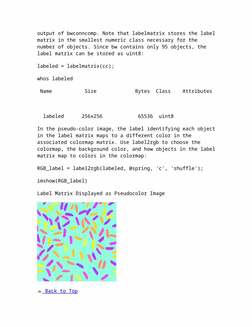
Step 9: View All Objects
One way to visualize connected components is to create a label matrix, and then display it as a pseudo-color indexed image. Uselabelmatrix to create a label matrix from the output of bwconncomp. Note that labelmatrix stores the label matrix in the smallest numeric class necessary for the number of objects. Since bw contains only 95 objects, the label matrix can be stored as uint8:
labeled = labelmatrix(cc);
whos labeled

Name Size Bytes Class Attributes
labeled 256x256 65536 uint8
In the pseudo-color image, the label identifying each object in the label matrix maps to a different color in the associated colormap matrix. Use label2rgb to choose the colormap, the background color, and how objects in the label matrix map to colors in the colormap:
RGB_label = label2rgb(labeled, @spring, 'c', 'shuffle');
imshow(RGB_label)
Label Matrix Displayed as Pseudocolor Image
Back to Top
Step 10: Compute Area of Each Object
Each rice grain is one connected component in the cc structure. Use regionprops on cc to compute the area.
graindata = regionprops(cc, 'basic')
MATLAB responds with
graindata =
95x1 struct array with fields:
Area
Centroid
BoundingBox
To find the area of the 50th component, use dot notation to access the Area field in the 50th element of graindata structure array:
graindata(50).Area
ans =
194
Back to Top
Step 11: Compute Area-based Statistics
Create a new vector allgrains to hold the area measurement for each grain:
grain_areas = [graindata.Area];
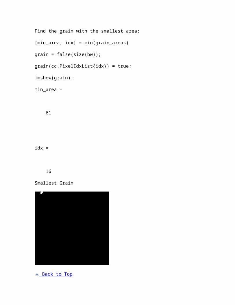
Find the grain with the smallest area:
[min_area, idx] = min(grain_areas)
grain = false(size(bw));
grain(cc.PixelIdxList{idx}) = true;
imshow(grain);
min_area =
61
idx =
16
Smallest Grain
Back to Top
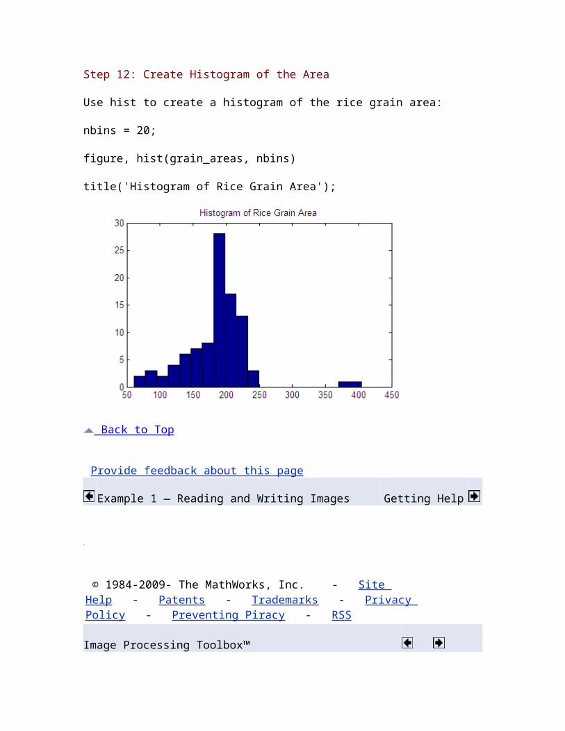
Step 12: Create Histogram of the Area
Use hist to create a histogram of the rice grain area:
nbins = 20;
figure, hist(grain_areas, nbins)
title('Histogram of Rice Grain Area');
Back to Top
Provide feedback about this page
Example 1 — Reading and Writing Images Getting Help
© 1984-2009- The MathWorks, Inc. - Site Help - Patents - Trademarks - Privacy Policy - Preventing Piracy - RSS
Image Processing Toolbox™
Provide feedback about this page
Getting Help
On this page…
Product Documentation
Image Processing Demos
MATLAB Newsgroup
Product Documentation
The Image Processing Toolbox documentation is available online in both HTML and PDF formats. To access the HTML help, select Help from the menu bar of the MATLAB desktop. In the Help Navigator pane, click the Contents tab and expand the Image Processing Toolboxtopic in the list.
To access the PDF help, click Image Processing Toolbox in the Contents tab of the Help browser and go to the link under Printable (PDF) Documentation on the Web. (Note that to view the PDF help, you must have Adobe® Acrobat® Reader installed.)
For reference information about any of the Image Processing Toolbox functions, see the online Functions — Alphabetical List, which complements the M-file help that is displayed in the MATLAB command window when you type
help functionname
For example,
help imtool
Back to Top
Image Processing Demos
The Image Processing Toolbox software is supported by a full complement of demo applications. These are very useful as templates for your own end-user applications, or for seeing how to use and combine your toolbox functions for powerful image analysis and enhancement.
To view all the demos, call the iptdemos function. This displays an HTML page in the MATLAB Help browser that lists all the demos.
You can also view this page by starting the MATLAB Help browser and clicking the Demos tab in the Help Navigator pane. From the list of products with demos, select Image Processing Toolbox.
The toolbox demos are located under the subdirectory
matlabroot\toolbox\images\imdemos
where matlabroot represents your MATLAB installation directory.
Back to Top
MATLAB Newsgroup
If you read newsgroups on the Internet, you might be interested in the MATLAB newsgroup (comp.soft-sys.matlab). This newsgroup gives you access to an active MATLAB user community. It is an excellent way to seek advice and to share algorithms, sample code, and M-files with other MATLAB users.
Back to Top
Provide feedback about this page
Example 2 — Analyzing Images Image Credits
© 1984-2009- The MathWorks, Inc. - Site Help - Patents - Trademarks - Privacy Policy - Preventing Piracy - RSS
Image Processing Toolbox™
Provide feedback about this page
Image Credits
This table lists the copyright owners of the images used in the Image Processing Toolbox documentation.
Image Source
Cameraman Copyright Massachusetts Institute of Technology. Used with permission.
Cell Cancer cell from a rat's prostate, courtesy of Alan W. Partin, M.D., Ph.D., Johns Hopkins University School of Medicine.
Circuit Micrograph of 16-bit A/D converter circuit, courtesy of Steve Decker and Shujaat Nadeem, MIT, 1993.

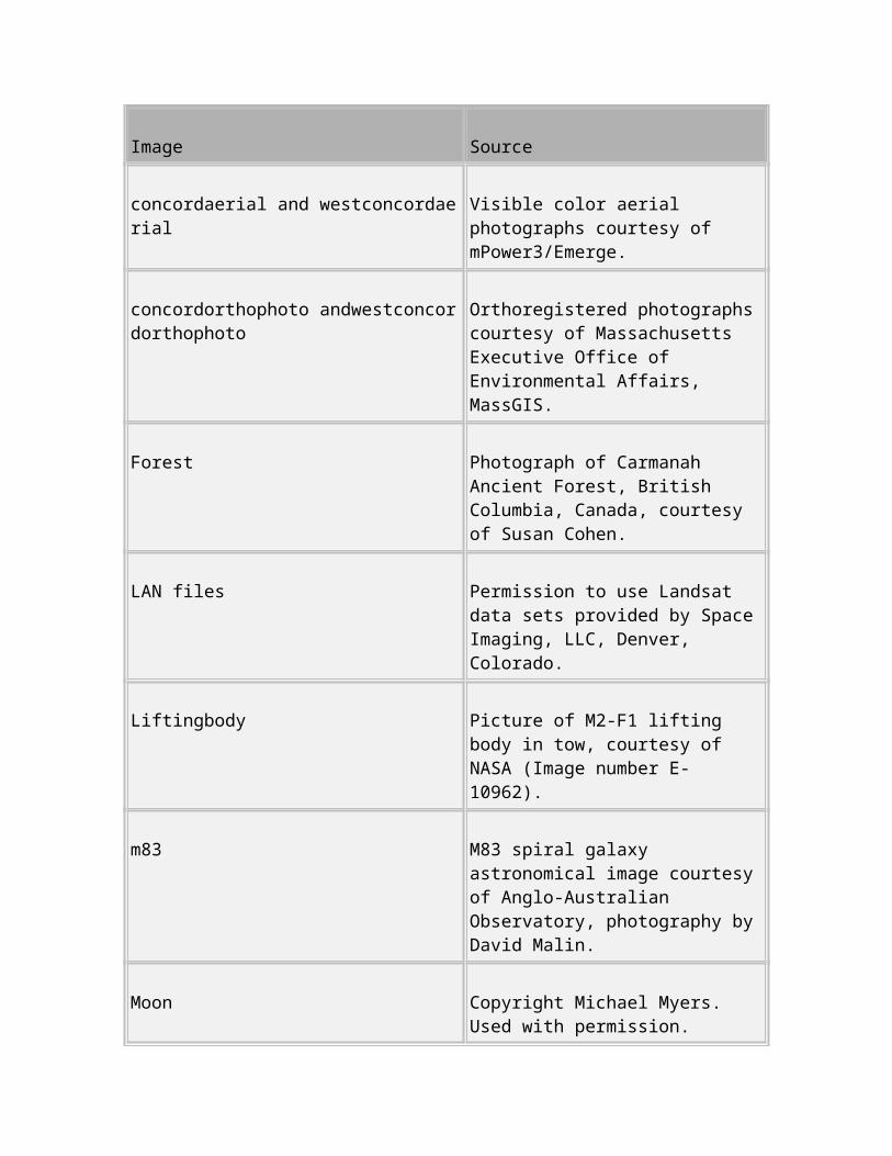
Image Source
concordaerial and westconcordaerial Visible color aerial photographs courtesy of mPower3/Emerge.
concordorthophoto andwestconcordorthophoto Orthoregistered photographs courtesy of Massachusetts Executive Office of Environmental Affairs, MassGIS.
Forest Photograph of Carmanah Ancient Forest, British Columbia, Canada, courtesy of Susan Cohen.
LAN files Permission to use Landsat data sets provided by Space Imaging, LLC, Denver, Colorado.
Liftingbody Picture of M2-F1 lifting body in tow, courtesy of NASA (Image number E-10962).
m83 M83 spiral galaxy astronomical image courtesy of Anglo-Australian Observatory, photography by David Malin.
Moon Copyright Michael Myers. Used with permission.
Saturn Voyager 2 image, 1981-08-24, NASA catalog #PIA01364.
Solarspectra Courtesy of Ann Walker. Used with permission.
Tissue Courtesy of Alan W. Partin, M.D., PhD., Johns Hopkins University School of Medicine.

Image Source
Trees Trees with a View, watercolor and ink on paper, copyright Susan Cohen. Used with permission.
Provide feedback about this page
Getting Help Examples
© 1984-2009- The MathWorks, Inc. - Site Help - Patents - Trademarks - Privacy Policy - Preventing Piracy - RSS
Image Processing Toolbox™
Provide feedback about this page
Examples
Use this list to find examples in the documentation.
Introductory Examples
Example 1 — Reading and Writing ImagesExample 2 — Analyzing Images
Image Representation and Storage
Getting Information About a Graphics FileReading Image DataWriting Image Data to a FileReading and Writing Binary Images in 1-Bit FormatReading Image Data from a DICOM FileCreating a New DICOM SeriesWorking with Mayo Analyze 7.5 FilesWorking with High Dynamic Range Images
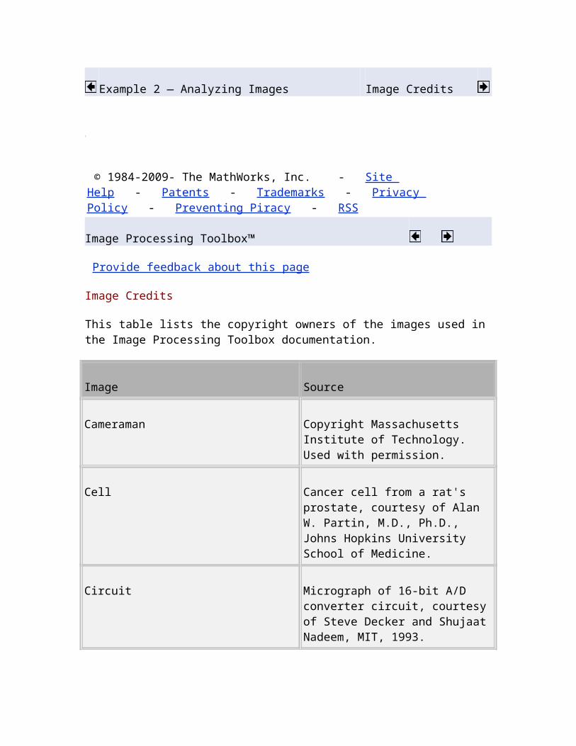
Image Display and Visualization
Displaying Images Using the imshow FunctionMoving the Detail Rectangle to Change the Image ViewPanning the Image Displayed in the Image ToolZooming In and Out on an Image in the Image ToolDetermining the Values of a Group of PixelsViewing a Sequence of MRI ImagesDisplaying Indexed ImagesDisplaying Grayscale ImagesDisplaying Grayscale Images That Have Unconventional RangesDisplaying Binary ImagesChanging the Display Colors of a Binary ImageDisplaying Truecolor ImagesAdding a Colorbar to a Displayed ImageBuilding a Navigation GUI for Large ImagesGetting Image Pixel Values Using impixelCreating an Intensity Profile of an Image Using improfileDisplaying a Contour Plot of Image Data
Zooming and Panning Images
Moving the Detail Rectangle to Change the Image ViewPanning the Image Displayed in the Image ToolZooming In and Out on an Image in the Image Tool
Pixel Values
Determining the Values of a Group of PixelsEmbedding the Pixel Region Tool in an Existing FigureBuilding a Pixel Information GUIGetting Image Pixel Values Using impixelCreating an Intensity Profile of an Image Using improfileDisplaying a Contour Plot of Image DataCreating an Image Histogram Using imhist
Image Measurement
Using the Distance ToolBuilding a Pixel Information GUICreating an Angle Measurement Tool
Image Enhancement
Adjusting Contrast with the Window/Level ToolPerforming Linear Filtering of Images Using imfilter
Filtering an Image with Predefined Filter TypesFilling HolesAdjusting Intensity Values to a Specified RangeAdjusting Intensity Values Using Histogram EqualizationAdjusting Intensity Values Using Contrast-Limited Adaptive Histogram EqualizationEnhancing Color Separation Using Decorrelation StretchingRemoving Noise By Median FilteringRemoving Noise By Adaptive FilteringFilling an ROIDeblurring with the Wiener FilterDeblurring with a Regularized FilterUsing the deconvlucy Function to Deblur an ImageUsing the deconvblind Function to Deblur an Image
Brightness and Contrast Adjustment
Adjusting Contrast with the Window/Level ToolAdjusting Intensity Values to a Specified RangeAdjusting Intensity Values Using Histogram EqualizationAdjusting Intensity Values Using Contrast-Limited Adaptive Histogram EqualizationFiltering a Region in an ImageSpecifying the Filtering Operation
Cropping Images
Cropping an Image Using the Crop Image ToolCropping an Image
GUI Application Development
Embedding the Pixel Region Tool in an Existing FigureBuilding a Pixel Information GUIBuilding a Navigation GUI for Large ImagesBuilding an Image Comparison ToolCreating an Angle Measurement Tool
Edge Detection
Building an Image Comparison ToolDetecting Lines Using the Radon TransformSkeletonizationPerimeter DeterminationDetecting Edges Using the edge FunctionTracing Object Boundaries in an Image
Regions of Interest (ROI)

Creating an Angle Measurement ToolCreating an ROI Without an Associated ImageSpecifying the Filtering Operation
Resizing Images
Resizing an Image
Image Registration and Alignment
Rotating an ImagePerforming a TranslationPerforming Image RegistrationRegistering to a Digital Orthophoto
Image Filters
Performing Linear Filtering of Images Using imfilter
Image Filtering
Filtering an Image with Predefined Filter TypesFiltering a Region in an ImageSpecifying the Filtering Operation
Image Transforms
Locating Image FeaturesDCT and Image CompressionDetecting Lines Using the Radon TransformReconstructing an Image from Parallel Projection DataReconstructing a Head Phantom Image
Fourier Transform
Locating Image Features
Feature Detection
Locating Image Features
Discrete Cosine Transform
DCT and Image Compression
Image Compression

DCT and Image Compression
Radon Transform
Detecting Lines Using the Radon TransformReconstructing an Image from Parallel Projection Data
Image Reconstruction
Reconstructing an Image from Parallel Projection DataReconstructing a Head Phantom Image
Fan-beam Transform
Reconstructing a Head Phantom Image
Morphological Operations
Creating a Structuring ElementDilating an ImageEroding an ImageMorphological OpeningSkeletonizationPerimeter DeterminationFilling Holes
Morphology Examples
Selecting Objects in a Binary ImageFinding the Area of the Foreground of a Binary Image
Image Histogram
Creating an Image Histogram Using imhist
Image Analysis
Detecting Edges Using the edge FunctionTracing Object Boundaries in an ImageDetecting Lines Using the Hough TransformAnalyzing Image Homogeneity Using Quadtree DecompositionUsing the Texture FunctionsPlotting the Correlation
Edge detection
Detecting Lines Using the Hough Transform
Hough Transform
Detecting Lines Using the Hough Transform
Image Texture
Using the Texture Functions
Image Statistics
Plotting the Correlation
Color Adjustment
Enhancing Color Separation Using Decorrelation StretchingReducing Colors Using imapproxDithering
Noise Reduction
Removing Noise By Median FilteringRemoving Noise By Adaptive Filtering
Regions of Interest
Filtering a Region in an Image
Filling Images
Filling an ROI
Deblurring Images
Deblurring with the Wiener FilterDeblurring with a Regularized FilterUsing the deconvlucy Function to Deblur an ImageUsing the deconvblind Function to Deblur an Image
Image Color
Reducing Colors Using imapproxDitheringPerforming a Color Space Conversion
Performing a Profile-Based ConversionConverting Between Device-Dependent Color Spaces
Color Space Conversion
Performing a Color Space ConversionPerforming a Profile-Based ConversionConverting Between Device-Dependent Color Spaces
Provide feedback about this page
© 1984-2009- The MathWorks, Inc. - Site Help - Patents - Trademarks - Privacy Policy - Preventing Piracy - RSS
Image Processing Toolbox™
Provide feedback about this page
Getting Information About a Graphics File
To obtain information about a graphics file and its contents, use the imfinfo function. You can use imfinfo with any of the formats supported by MATLAB. Use the imformats function to determine which formats are supported.
Note You can also get information about an image displayed in the Image Tool — see Getting Information About an Image Using the Image Information Tool.
The information returned by imfinfo depends on the file format, but it always includes at least the following:
Name of the file
File format
Version number of the file format
File modification date
File size in bytes
Image width in pixels
Image height in pixels
Number of bits per pixel
Image type: truecolor (RGB), grayscale (intensity), or indexed
Provide feedback about this page
Reading and Writing Image Data Reading Image Data
© 1984-2009- The MathWorks, Inc. - Site Help - Patents - Trademarks - Privacy Policy - Preventing Piracy - RSS
Image Processing Toolbox™
Provide feedback about this page
Reading Image Data
To import an image from any supported graphics image file format, in any of the supported bit depths, use the imread function. This example reads a truecolor image into the MATLAB workspace as the variable RGB.
RGB = imread('football.jpg');
If the image file format uses 8-bit pixels, imread stores the data in the workspace as a uint8 array. For file formats that support 16-bit data, such as PNG and TIFF, imread creates a uint16 array.
imread uses two variables to store an indexed image in the workspace: one for the image and another for its associated colormap. imreadalways reads the colormap into a matrix of class double, even though the image array itself may be of class uint8 or uint16.
[X,map] = imread('trees.tif');
In these examples, imread infers the file format to use from the contents of the file. You can also specify the file format as an argument toimread. imread supports many common

graphics file formats, such as Microsoft® Windows® Bitmap (BMP), Graphics Interchange Format (GIF), Joint Photographic Experts Group (JPEG), Portable Network Graphics (PNG), and Tagged Image File Format (TIFF) formats. For the latest information concerning the bit depths and/or image formats supported, see imread and imformats.
If the graphics file contains multiple images, imread imports only the first image from the file. To import additional images, you must useimread with format-specific arguments to specify the image you want to import. In this example, imread imports a series of 27 images from a TIFF file and stores the images in a four-dimensional array. You can use imfinfo to determine how many images are stored in the file.
mri = zeros([128 128 1 27],'uint8'); % preallocate 4-D array
for frame=1:27
[mri(:,:,:,frame),map] = imread('mri.tif',frame);
end
When a file contains multiple images that are related in some way, you can call image processing algorithms directly. . For more information, see Working with Image Sequences.
Provide feedback about this page
Getting Information About a Graphics File Writing Image Data to a File
© 1984-2009- The MathWorks, Inc. - Site Help - Patents - Trademarks - Privacy Policy - Preventing Piracy - RSS
Image Processing Toolbox™
Provide feedback about this page
Writing Image Data to a File
On this page…
Overview
Specifying Format-Specific Parameters
Reading and Writing Binary Images in 1-Bit Format
Determining the Storage Class of the Output File
Overview
To export image data from the MATLAB workspace to a graphics file in one of the supported graphics file formats, use the imwritefunction. When using imwrite, you specify the MATLAB variable name and the name of the file. If you include an extension in the filename,imwrite attempts to infer the desired file format from it. For example, the file extension .jpg infers the Joint Photographic Experts Group (JPEG) format. You can also specify the format explicitly as an argument to imwrite.
This example loads the indexed image X from a MAT-file, clown.mat, along with the associated colormap map, and then exports the image as a bitmap (BMP) file.
load clown
whos
Name Size Bytes Class
X 200x320 512000 double array
caption 2x1 4 char array
map 81x3 1944 double array
Grand total is 64245 elements using 513948 bytes
imwrite(X,map,'clown.bmp')
Back to Top

Specifying Format-Specific Parameters
When using imwrite with some graphics formats, you can specify additional format-specific parameters. For example, with PNG files, you can specify the bit depth. This example writes a grayscale image I to a 4-bit PNG file.
imwrite(I,'clown.png','BitDepth',4);
This example writes an image A to a JPEG file, using an additional parameter to specify the compression quality parameter.
imwrite(A, 'myfile.jpg', 'Quality', 100);
For more information about these additional format-specific syntaxes, see the imwrite reference page.
Back to Top
Reading and Writing Binary Images in 1-Bit Format
In certain file formats, such as TIFF, a binary image can be stored in a 1-bit format. When you read in a binary image in 1-bit format,imread stores the data in the workspace as a logical array. If the file format supports it, imwrite writes binary images as 1-bit images by default. This example reads in a binary image and writes it as a TIFF file.
BW = imread('text.png');
imwrite(BW,'test.tif');
To verify the bit depth of test.tif, call imfinfo and check the BitDepth field.
info = imfinfo('test.tif');
info.BitDepth
ans =
1
Note When writing binary files, MATLAB sets the ColorType field to 'grayscale'.
Back to Top
Determining the Storage Class of the Output File
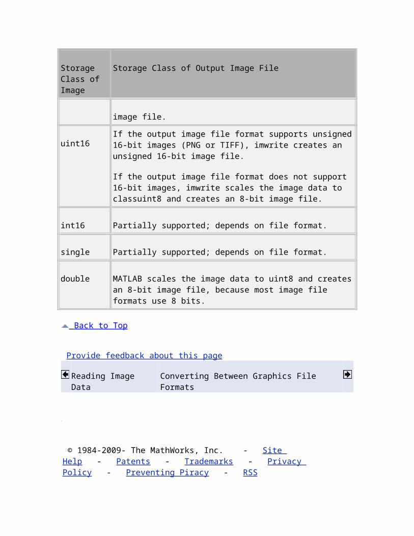
imwrite uses the following rules to determine the storage class used in the output image.
Storage Class of Image
Storage Class of Output Image File
logicalIf the output image file format supports 1-bit images, imwrite creates a 1-bit image file.
If the output image file format specified does not support 1-bit images, imwrite exports the image data as a uint8 grayscale image.
uint8 If the output image file format supports unsigned 8-bit images, imwrite creates an unsigned 8-bit image file.
uint16If the output image file format supports unsigned 16-bit images (PNG or TIFF), imwrite creates an unsigned 16-bit image file.
If the output image file format does not support 16-bit images, imwrite scales the image data to classuint8 and creates an 8-bit image file.
int16 Partially supported; depends on file format.
single Partially supported; depends on file format.
double MATLAB scales the image data to uint8 and creates an 8-bit image file, because most image file formats use 8 bits.
Back to Top
Provide feedback about this page
Reading Image Data Converting Between Graphics File Formats
© 1984-2009- The MathWorks, Inc. - Site Help - Patents - Trademarks - Privacy Policy - Preventing Piracy - RSS
Image Processing Toolbox™
Provide feedback about this page
Converting Between Graphics File Formats
To change the graphics format of an image, use imread to import the image into the MATLAB workspace and then use the imwrite function to export the image, specifying the appropriate file format.
To illustrate, this example uses the imread function to read an image in TIFF format into the workspace and write the image data as JPEG format.
moon_tiff = imread('moon.tif');
imwrite(moon_tiff,'moon.jpg');
For the specifics of which bit depths are supported for the different graphics formats, and for how to specify the format type when writing an image to file, see the reference pages for imread and imwrite.
Provide feedback about this page
Writing Image Data to a File Working with DICOM Files
© 1984-2009- The MathWorks, Inc. - Site Help - Patents - Trademarks - Privacy Policy - Preventing Piracy - RSS
Image Processing Toolbox™
Provide feedback about this page
Displaying and Exploring Images

This section describes the image display and exploration tools provided by the Image Processing Toolbox software.
Overview
Displaying Images Using the imshow Function
Using the Image Tool to Explore Images
Exploring Very Large Images
Using Image Tool Navigation Aids
Getting Information about the Pixels in an Image
Measuring the Distance Between Two Pixels
Getting Information About an Image Using the Image Information Tool
Adjusting Image Contrast Using the Adjust Contrast Tool
Cropping an Image Using the Crop Image Tool
Viewing Image Sequences
Displaying Different Image Types
Adding a Colorbar to a Displayed Image
Printing Images
Setting Toolbox Preferences
Provide feedback about this page
Working with High Dynamic Range Images Overview
© 1984-2009- The MathWorks, Inc. - Site Help - Patents - Trademarks - Privacy Policy - Preventing Piracy - RSS
Image Processing Toolbox™

Provide feedback about this page
Overview
The Image Processing Toolbox software includes two display functions, imshow and imtool. Both functions work within the Handle Graphics architecture: they create an image object and display it in an axes object contained in a figure object.
imshow is the toolbox's fundamental image display function. Use imshow when you want to display any of the different image types supported by the toolbox, such as grayscale (intensity), truecolor (RGB), binary, and indexed. For more information, see Displaying Images Using the imshow Function. The imshow function is also a key building block for image applications you can create using the toolbox modular tools. For more information, see Building GUIs with Modular Tools.
The other toolbox display function, imtool, launches the Image Tool, which presents an integrated environment for displaying images and performing some common image-processing tasks. The Image Tool provides all the image display capabilities of imshow but also provides access to several other tools for navigating and exploring images, such as scroll bars, the Pixel Region tool, the Image Information tool, and the Adjust Contrast tool. For more information, see Using the Image Tool to Explore Images.
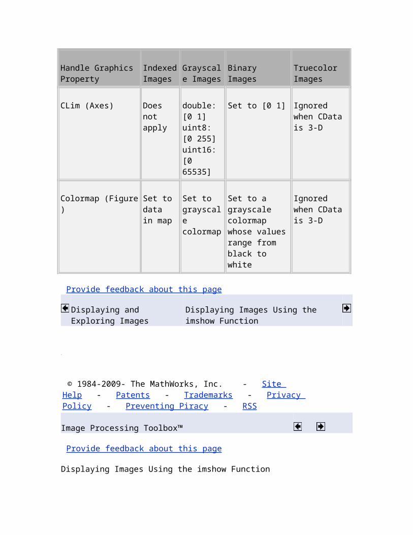
In general, using the toolbox functions to display images is preferable to using MATLAB image display functions image and imagescbecause the toolbox functions set certainHandle Graphics properties automatically to optimize the image display. The following table lists these properties and their settings for each image type. In the table, X represents an indexed image, I represents a grayscale image, BWrepresents a binary image, and RGB represents a truecolor image.
Note Both imshow and imtool can perform automatic scaling of image data. When called with the syntaximshow(I,'DisplayRange',[]), and similarly for imtool, the functions set the axes CLim property to [min(I(:)) max(I(:))].CDataMapping is always scaled for grayscale images, so that the value min(I(:)) is displayed using the first colormap color, and the value max(I(:)) is displayed using the last colormap color.
Handle Graphics Property
Indexed Images
Grayscale Images
Binary Images Truecolor Images
CData (Image) Set to the data in X
Set to the data in I
Set to data in BW Set to data in RGB
Handle Graphics Property
Indexed Images
Grayscale Images
Binary Images Truecolor Images
CDataMapping (Image) Set to 'direct'
Set to 'scaled'
Set to 'direct' Ignored when CData is 3-D
CLim (Axes) Does not apply
double: [0 1] uint8: [0 255] uint16: [0 65535]
Set to [0 1] Ignored when CData is 3-D
Colormap (Figure) Set to data in map
Set to grayscale colormap
Set to a grayscale colormap whose values range from black to white
Ignored when CData is 3-D
Provide feedback about this page
Displaying and Exploring Images Displaying Images Using the imshow Function
© 1984-2009- The MathWorks, Inc. - Site Help - Patents - Trademarks - Privacy Policy - Preventing Piracy - RSS
Image Processing Toolbox™
Provide feedback about this page
Displaying Images Using the imshow Function
On this page…
Overview

Specifying the Initial Image Magnification
Controlling the Appearance of the Figure
Displaying Each Image in a Separate Figure
Displaying Multiple Images in the Same Figure
Overview
To display image data, use the imshow function. The following example reads an image into the MATLAB workspace and then displays the image in a MATLAB figure window.
moon = imread('moon.tif');
imshow(moon);
The imshow function displays the image in a MATLAB figure window, as shown in the following figure.
Image Displayed in a Figure Window by imshow
You can also pass imshow the name of a file containing an image.
imshow('moon.tif');
This syntax can be useful for scanning through images. Note, however, that when you use this syntax, imread does not store the image data in the MATLAB workspace. If you want to bring the image into the workspace, you must use the getimage function, which retrieves the image data from the current Handle Graphics image object. This example assigns the image data from moon.tif to the variable moon, if the figure window in which it is displayed is currently active.
moon = getimage;
For more information about using imshow to display the various image types supported by the toolbox, see Displaying Different Image Types.
Back to Top
Specifying the Initial Image Magnification
By default, imshow attempts to display an image in its entirety at 100% magnification (one screen pixel for each image pixel). However, if an image is too large to fit in a figure window on the screen at 100% magnification, imshow scales the image to fit onto the screen and issues a warning message.
To override the default initial magnification behavior for a particular call to imshow, specify the InitialMagnification parameter. For example, to view an image at 150% magnification, use this code.
pout = imread('pout.tif');
imshow(pout, 'InitialMagnification', 150)
imshow attempts to honor the magnification you specify. However, if the image does not fit on the screen at the specified magnification,imshow scales the image to fit and issues a warning message. You can also specify the text string 'fit' as the initial magnification value. In this case, imshow scales the image to fit the current size of the figure window.
To change the default initial magnification behavior of imshow, set the ImshowInitialMagnification toolbox preference. To set the preference, open the Image Processing Toolbox Preferences dialog by calling iptprefs or by selecting Preferences from the MATLAB Desktop File menu.
When imshow scales an image, it uses interpolation to determine the values for screen pixels that do not directly correspond to elements in the image matrix. For more information, see Specifying the Interpolation Method.
Back to Top
Controlling the Appearance of the Figure
By default, when imshow displays an image in a figure, it surrounds the image with a gray border. You can change this default and suppress the border using the 'border' parameter, as shown in the following example.
imshow('moon.tif','Border','tight')
The following figure shows the same image displayed with and without a border.
Image Displayed With and Without a Border

The 'border' parameters affect only the image being displayed in the call to imshow. If you want all the images that you display usingimshow to appear without the gray border, set the Image Processing Toolbox 'ImshowBorder' preference to 'tight'. You can also use preferences to include visible axes in the figure. For more information about preferences, see iptprefs.
Back to Top
Displaying Each Image in a Separate Figure
The simplest way to display multiple images is to display them in separate figure windows. MATLAB does not place any restrictions on the number of images you can display simultaneously.
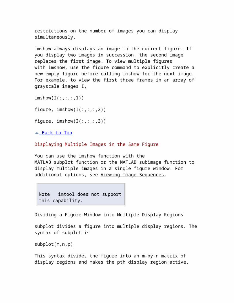
imshow always displays an image in the current figure. If you display two images in succession, the second image replaces the first image. To view multiple figures with imshow, use the figure command to explicitly create a new empty figure before
calling imshow for the next image. For example, to view the first three frames in an array of grayscale images I,
imshow(I(:,:,:,1))
figure, imshow(I(:,:,:,2))
figure, imshow(I(:,:,:,3))
Back to Top
Displaying Multiple Images in the Same Figure
You can use the imshow function with the MATLAB subplot function or the MATLAB subimage function to display multiple images in a single figure window. For additional options, see Viewing Image Sequences.
Note imtool does not support this capability.
Dividing a Figure Window into Multiple Display Regions
subplot divides a figure into multiple display regions. The syntax of subplot is
subplot(m,n,p)
This syntax divides the figure into an m-by-n matrix of display regions and makes the pth display region active.
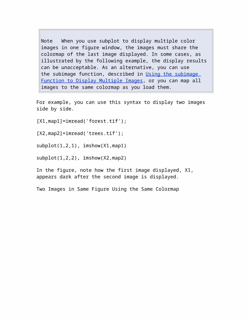
Note When you use subplot to display multiple color images in one figure window, the images must share the colormap of the last image displayed. In some cases, as illustrated by the following example, the display results can be unacceptable. As an alternative, you can use the subimage function, described in Using the subimage Function to Display Multiple Images, or you can map all images to the same colormap as you load them.
For example, you can use this syntax to display two images side by side.
[X1,map1]=imread('forest.tif');
[X2,map2]=imread('trees.tif');
subplot(1,2,1), imshow(X1,map1)

subplot(1,2,2), imshow(X2,map2)
In the figure, note how the first image displayed, X1, appears dark after the second image is displayed.
Two Images in Same Figure Using the Same Colormap
Using the subimage Function to Display Multiple Images
subimage converts images to truecolor before displaying them and therefore circumvents the colormap sharing problem. This example uses subimage to display the forest and the trees images with better results.
[X1,map1]=imread('forest.tif');
[X2,map2]=imread('trees.tif');
subplot(1,2,1), subimage(X1,map1)
subplot(1,2,2), subimage(X2,map2)
Two Images in Same Figure Using Separate Colormaps
Back to Top
Provide feedback about this page
Overview Using the Image Tool to Explore Images
© 1984-2009- The MathWorks, Inc. - Site Help - Patents - Trademarks - Privacy Policy - Preventing Piracy - RSS
Image Processing Toolbox™
Provide feedback about this page
Using the Image Tool to Explore Images
On this page…
Image Tool Overview

Opening the Image Tool
Specifying the Initial Image Magnification
Specifying the Colormap
Importing Image Data from the Workspace
Exporting Image Data to the Workspace
Saving the Image Data Displayed in the Image Tool
Closing the Image Tool
Printing the Image in the Image Tool
Image Tool Overview
The Image Tool is an image display and exploration tool that presents an integrated environment for displaying images and performing common image-processing tasks. The Image Tool provides access to several other tools:
Pixel Information tool — for getting information about the pixel under the pointer
Pixel Region tool — for getting information about a group of pixels
Distance tool — for measuring the distance between two pixels
Image Information tool — for getting information about image and image file metadata
Adjust Contrast tool and associated Window/Level tool — for adjusting the contrast of the image displayed in the Image Tool and modifying the actual image data. You can save the adjusted data to the workspace or a file.
Crop Image tool — for defining a crop region on the image and cropping the image. You can save the cropped image to the workspace or a file.
Display Range tool — for determining the display range of the image data
In addition, the Image Tool provides several navigation aids that can help explore large images:
Overview tool — for determining what part of the image is currently visible in the Image Tool and changing this view.

Pan tool — for moving the image to view other parts of the image
Zoom tool — for getting a closer view of any part of the image.
Scroll bars — for navigating over the image.
The following figure shows the image displayed in the Image Tool with many of the related tools open and active.
Image Tool and Related Tools
Back to Top
Opening the Image Tool
To start the Image Tool, use the imtool function. You can also start another Image Tool from within an existing Image Tool by using theNew option from the File menu.
The imtool function supports many syntax options. For example, when called without any arguments, it opens an empty Image Tool.
imtool
To bring image data into this empty Image Tool, you can use either the Open or Import from Workspace options from the File menu — see Importing Image Data from the Workspace.
You can also specify the name of the MATLAB workspace variable that contains image data when you call imtool, as follows:
moon = imread('moon.tif');
imtool(moon)
Alternatively, you can specify the name of the graphics file containing the image. This syntax can be useful for scanning through graphics files.
imtool('moon.tif');
Note When you use this syntax, the image data is not stored in a MATLAB workspace variable. To bring the image displayed in the Image Tool into the workspace, you must use the getimage function or the Export from Workspace option from the Image ToolFile menu — see Exporting Image Data to the Workspace.
Back to Top
Specifying the Initial Image Magnification
The imtool function attempts to display an image in its entirety at 100% magnification (one screen pixel for each image pixel) and always honors any magnification value you specify. If the image is too big to fit in a figure on the screen, the Image Tool shows only a portion of the image, adding scroll bars to allow navigation to parts of the image that are not currently visible. If the specified magnification would make the image too large to fit on the screen, imtool scales the image to fit, without issuing a warning. This is the default behavior, specified by the imtool 'InitialMagnification' parameter value 'adaptive'.
To override this default initial magnification behavior for a particular call to imtool, specify the InitialMagnification parameter. For example, to view an image at 150% magnification, use this code.

pout = imread('pout.tif');
imtool(pout, 'InitialMagnification', 150)
You can also specify the text string 'fit' as the initial magnification value. In this case, imtool scales the image to fit the default size of a figure window.
Another way to change the default initial magnification behavior of imtool is to set the ImtoolInitialMagnification toolbox preference. The magnification value you specify will remain in effect until you change it. To set the preference, use iptsetpref or open the Image Processing Preferences panel by calling iptprefs or by selecting File > Preferencesin the Image Tool menu. To learn more about toolbox preferences, see iptprefs.
When imtool scales an image, it uses interpolation to determine the values for screen pixels that do not directly correspond to elements in the image matrix. For more information, see Specifying the Interpolation Method.
Back to Top
Specifying the Colormap
A colormap is a matrix that can have any number of rows, but must have three columns. Each row in the colormap is interpreted as a color, with the first element specifying the intensity of red, the second green, and the third blue.
To specify the color map used to display an indexed image or a grayscale image in the Image Tool, select the Choose Colormap option on the Tools menu. This activates the Choose Colormap tool. Using this tool you can select one of the MATLAB colormaps or select a colormap variable from the MATLAB workspace.
When you select a colormap, the Image Tool executes the colormap function you specify and updates the image displayed. You can edit the colormap command in the Evaluate Colormap text box; for example, you can change the number of entries in the colormap (default is 256). You can enter your own colormap function in this field. Press Enter to execute the command.
When you choose a colormap, the image updates to use the new map. If you click OK, the Image Tool applies the colormap and closes the Choose Colormap tool. If you click Cancel, the image reverts to the previous colormap.
Image Tool Choose Colormap Tool

Back to Top
Importing Image Data from the Workspace
To import image data from the MATLAB workspace into the Image Tool, use the Import from Workspace option on the Image Tool Filemenu. In the dialog box, shown below, you select the workspace variable that you want to import into the workspace.
The following figure shows the Import from Workspace dialog box. You can use the Filter menu to limit the images included in the list to certain image types, i.e., binary, indexed, intensity (grayscale), or truecolor.
Image Tool Import from Workspace Dialog Box
Back to Top
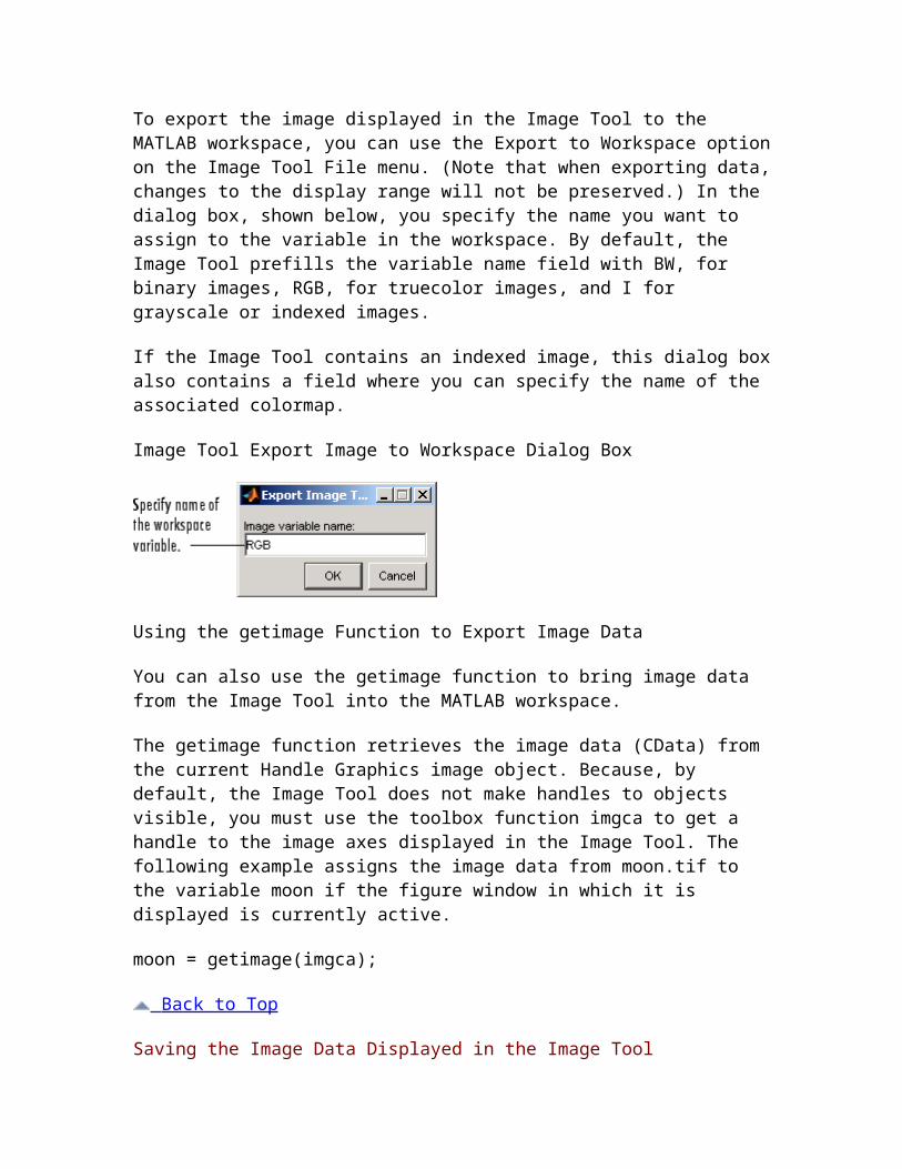
Exporting Image Data to the Workspace
To export the image displayed in the Image Tool to the MATLAB workspace, you can use the Export to Workspace option on the Image Tool File menu. (Note that when exporting data, changes to the display range will not be preserved.) In the dialog box, shown below, you specify the name you want to assign to the variable in the workspace. By default, the Image Tool prefills the variable name field with BW, for binary images, RGB, for truecolor images, and I for grayscale or indexed images.
If the Image Tool contains an indexed image, this dialog box also contains a field where you can specify the name of the associated colormap.
Image Tool Export Image to Workspace Dialog Box
Using the getimage Function to Export Image Data
You can also use the getimage function to bring image data from the Image Tool into the MATLAB workspace.
The getimage function retrieves the image data (CData) from the current Handle Graphics image object. Because, by default, the Image Tool does not make handles to objects visible, you must use the toolbox function imgca to get a handle to the image axes displayed in the Image Tool. The following example assigns the image data from moon.tif to the variable moon if the figure window in which it is displayed is currently active.
moon = getimage(imgca);
Back to Top
Saving the Image Data Displayed in the Image Tool
To save the image data displayed in the Image Tool, select the Save as option from the Image Tool File menu. The Image Tool opens the Save Image dialog box, shown in the following figure. Use this dialog box to navigate your file system to determine where to save the image file and specify the name of the file. Choose the graphics file format you want to use from among many common image file formats listed in the Files of Type menu. If you do not specify a file name extension, the Image Tool adds an extension to the file associated with the file format selected, such as .jpg for the JPEG format.
Image Tool Save Image Dialog Box

Note Changes you make to the display range will not be saved. If you would like to preserve your changes, use imcontrast.
Back to Top
Closing the Image Tool
To close the Image Tool window, use the Close button in the window title bar or select the Close option from the Image Tool File menu. You can also use the imtool function to return a handle to the Image Tool and use the handle to close the Image Tool. When you close the Image Tool, any related tools that are currently open also close.
Because the Image Tool does not make the handles to its figure objects visible, the Image Tool does not close when you call the MATLABclose all command. If you want to close multiple Image Tools, use the syntax
imtool close all
or select Close all from the Image Tool File menu.
Back to Top
Printing the Image in the Image Tool
To print the image displayed in the Image Tool, select the Print to Figure option from the File menu. The Image Tool opens another figure window and displays the image. Use the Print option on the File menu of this figure window to print the image. See Printing Imagesfor more information.
Back to Top
Provide feedback about this page
Displaying Images Using the imshow Function Exploring Very Large Images
© 1984-2009- The MathWorks, Inc. - Site Help - Patents - Trademarks - Privacy Policy - Preventing Piracy - RSS
Image Processing Toolbox™

Provide feedback about this page
Exploring Very Large Images
On this page…
Overview
Creating an R-Set File
Opening an R-Set File
Overview
If you are viewing a very large image, it might not load in imtool, or it could load, but zooming and panning are slow. In either case, creating a reduced resolution data set (R-Set) can improve performance. Use imtool to navigate an R-Set image the same way you navigate a standard image.
Back to Top
Creating an R-Set File
To create an R-Set file from a TIFF image file, use the function rsetwrite. For example, to create an R-Set from a TIFF file called'LargeImage.tif', enter the following:
rsetfile = rsetwrite ('LargeImage.tif')
rsetwrite saves an R-Set file named 'LargeImage.rset' in the current directory. Or, if you want to save the R-Set file under a different name, enter the following:
rsetfile = rsetwrite('LargeImage.tif', 'New_Name')
The time required to create an R-Set varies, depending on the size of the initial file and the capability of your machine. A progress bar shows an estimate of time required. If you cancel the operation, processing stops, no file is written, and the rsetfile variable will be empty.
Back to Top
Opening an R-Set File
You can open an R-Set file from the command line, or directly in the Image Tool. From the command line, type:
imtool('LargeImage.rset')
From the Image Tool, select File > Open From R-Set.
Back to Top
Provide feedback about this page
Using the Image Tool to Explore Images Using Image Tool Navigation Aids
© 1984-2009- The MathWorks, Inc. - Site Help - Patents - Trademarks - Privacy Policy - Preventing Piracy - RSS
Image Processing Toolbox™
Provide feedback about this page
Using Image Tool Navigation Aids
On this page…
Navigating an Image Using the Overview Tool
Panning the Image Displayed in the Image Tool
Zooming In and Out on an Image in the Image Tool
Specifying the Magnification of the Image
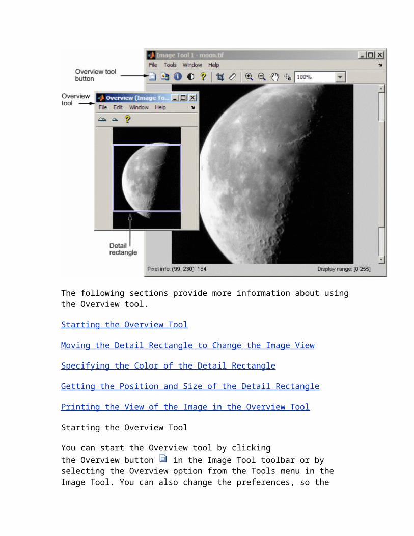
Navigating an Image Using the Overview Tool
If an image is large or viewed at a large magnification, the Image Tool displays only a portion of the entire image, including scroll bars to allow navigation around the image. To determine which part of the image is currently visible in the Image Tool, use the Overview tool. The Overview tool displays the entire image, scaled to fit. Superimposed over this view of the image is a rectangle, called the detail rectangle. The detail rectangle shows which part of the image is currently visible in the Image Tool. You can change the portion of the image visible in the Image Tool by moving the detail rectangle over the image in the Overview tool.
Image Tool with Overview Tool
The following sections provide more information about using the Overview tool.
Starting the Overview Tool
Moving the Detail Rectangle to Change the Image View
Specifying the Color of the Detail Rectangle
Getting the Position and Size of the Detail Rectangle
Printing the View of the Image in the Overview Tool
Starting the Overview Tool
You can start the Overview tool by clicking the Overview button in the Image Tool toolbar or by selecting the Overview option from the Tools menu in the Image Tool. You can also change the preferences, so the Overview tool will open automatically when you open the Image Tool. For more information on setting preferences, see iptprefs.

Moving the Detail Rectangle to Change the Image View
Start the Overview tool by clicking the Overview button in the Image Tool toolbar or by selecting Overview from the Toolsmenu. The Overview tool opens in a separate window containing a view of the entire image, scaled to fit.
If the Overview tool is already active, clicking the Overview button brings the tool to the front of the windows open on your screen.
Using the mouse, move the pointer into the detail rectangle. The pointer changes to a
fleur, .
Press and hold the mouse button to drag the detail rectangle anywhere on the image. The Image Tool updates the view of the image to make the specified region visible.
Specifying the Color of the Detail Rectangle
By default, the color of the detail rectangle in the Overview tool is blue. You can change the color of the rectangle to achieve better contrast with the predominant color of the underlying image. To do this, right-click anywhere inside the boundary of the detail rectangle and select a color from the Set Color option on the context menu.
Getting the Position and Size of the Detail Rectangle
To get the current position and size of the detail rectangle, right-click anywhere inside it and select Copy Position from the context menu. You can also access this option from the Edit menu of the Overview tool.
This option copies the position information to the clipboard. The position information is a vector of the form [xmin ymin width height]. You can paste this position vector into the MATLAB workspace or another application.
Printing the View of the Image in the Overview Tool
You can print the view of the image displayed in the Overview tool. Select the Print to Figure option from the Overview tool File menu. See Printing Images for more information.
Back to Top
Panning the Image Displayed in the Image Tool
To change the portion of the image displayed in the Image Tool, you can use the Pan tool to move the image displayed in the window. This is called panning the image.

Click the Pan tool button in the toolbar or select Pan from the Tools menu. When the Pan tool is active, a checkmark appears next to the Pan selection in the menu.
Move the pointer over the image in the Image Tool, using the mouse. The pointer changes to an open-hand shape .
Press and hold the mouse button and drag the image in the Image Tool. When you drag the image, the pointer changes to the closed-hand shape .
To turn off panning, click the Pan tool button again or click the Pan option in the Tools menu.
Note As you pan the image in the Image Tool, the Overview tool updates the position of the detail rectangle — see Navigating an Image Using the Overview Tool.
Back to Top
Zooming In and Out on an Image in the Image Tool
To enlarge an image to get a closer look or shrink an image to see the whole image in context, use the Zoom buttons on the toolbar. (You can also zoom in or out on an image by changing the magnification — see Specifying the Magnification of the Image or by using theCtrl+Plus or Ctrl+Minus keys. Note that these are the Plus(+) and Minus(-) keys on the numeric keypad of your keyboard.)
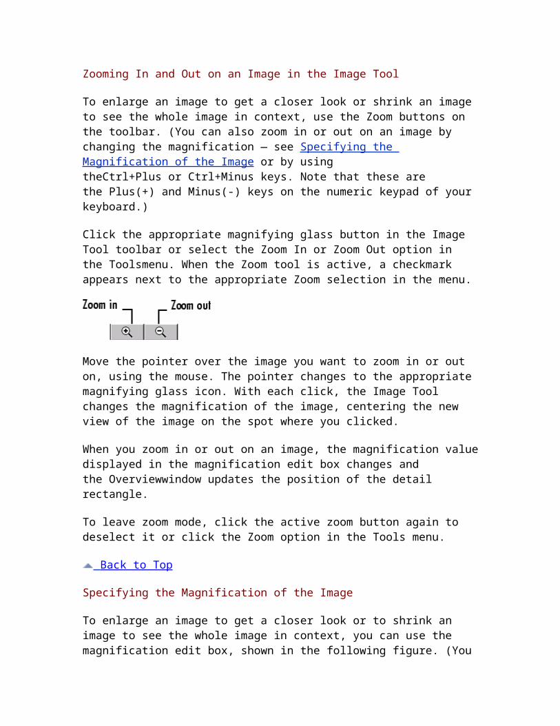
Click the appropriate magnifying glass button in the Image Tool toolbar or select the Zoom In or Zoom Out option in the Toolsmenu. When the Zoom tool is active, a checkmark appears next to the appropriate Zoom selection in the menu.
Move the pointer over the image you want to zoom in or out on, using the mouse. The pointer changes to the appropriate magnifying glass icon. With each click, the Image Tool changes the magnification of the image, centering the new view of the image on the spot where you clicked.
When you zoom in or out on an image, the magnification value displayed in the magnification edit box changes and the Overviewwindow updates the position of the detail rectangle.

To leave zoom mode, click the active zoom button again to deselect it or click the Zoom option in the Tools menu.
Back to Top
Specifying the Magnification of the Image
To enlarge an image to get a closer look or to shrink an image to see the whole image in context, you can use the magnification edit box, shown in the following figure. (You can also use the Zoom buttons to enlarge or shrink an image. See Zooming In and Out on an Image in the Image Tool for more information.)
Image Tool Magnification Edit Box and Menu
To change the magnification of an image,

Move the pointer into the magnification edit box. The pointer changes to the text entry cursor.
Type a new value in the magnification edit box and press Enter. The Image Tool changes the magnification of the image and displays the new view in the window.
You can also specify a magnification by clicking the menu associated with the magnification edit box and selecting from a list of preset magnifications. If you choose the Fit to Window option, the Image Tool scales the image so that the entire image is visible.
Back to Top
Provide feedback about this page
Exploring Very Large Images Getting Information about the Pixels in an Image
© 1984-2009- The MathWorks, Inc. - Site Help - Patents - Trademarks - Privacy Policy - Preventing Piracy - RSS
Image Processing Toolbox™
Provide feedback about this page
Getting Information about the Pixels in an Image
On this page…
Determining the Value of Individual Pixels
Determining the Values of a Group of Pixels
Determining the Display Range of an Image
Determining the Value of Individual Pixels
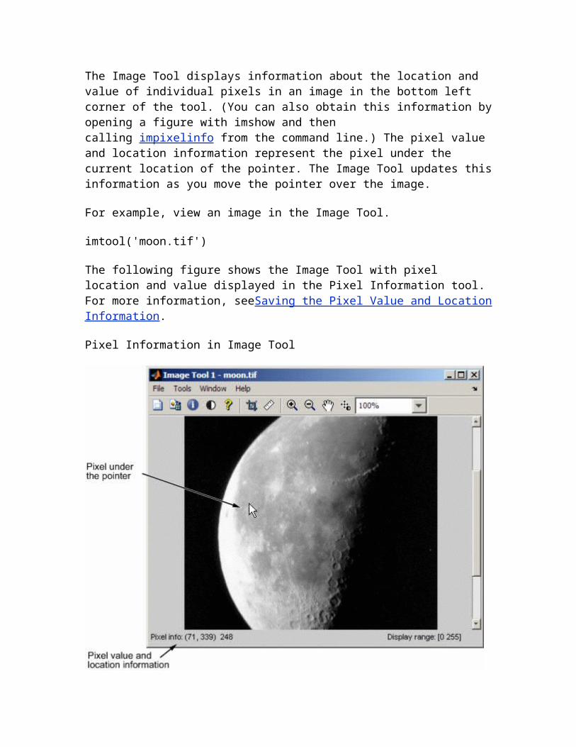
The Image Tool displays information about the location and value of individual pixels in an image in the bottom left corner of the tool. (You can also obtain this information by opening a figure with imshow and then calling impixelinfo from the command line.) The pixel value and location information represent the pixel under the current location of the

pointer. The Image Tool updates this information as you move the pointer over the image.
For example, view an image in the Image Tool.
imtool('moon.tif')
The following figure shows the Image Tool with pixel location and value displayed in the Pixel Information tool. For more information, seeSaving the Pixel Value and Location Information.
Pixel Information in Image Tool
Saving the Pixel Value and Location Information
To save the pixel location and value information displayed, right-click a pixel in the image and choose the Copy pixel info option. The Image Tool copies the x- and y-coordinates and the pixel value to the clipboard.
To paste this pixel information into the MATLAB workspace or another application, right-click and select Paste from the context menu.
Back to Top
Determining the Values of a Group of Pixels
To view the values of pixels in a specific region of an image displayed in the Image Tool, use the Pixel Region tool. The Pixel Region tool superimposes a rectangle, called the pixel region rectangle, over the image displayed in the Image Tool. This rectangle defines the group of pixels that are displayed, in extreme close-up view, in the Pixel Region tool window. The following figure shows the Image Tool with the Pixel Region tool. Note how the Pixel Region tool includes the value of each pixel in the display.
The following sections provide more information about using the Pixel Region tool.
Selecting a Region
Customizing the View
Determining the Location of the Pixel Region Rectangle
Printing the View of the Image in the Pixel Region Tool

Selecting a Region
To start the Pixel Region tool, click the Pixel Region button in the Image Tool toolbar or select the Pixel Region option from theTools menu. (Another option is to open a figure using imshow and then call impixelregion from the command line.) The Image Tool
displays the pixel region rectangle in the center of the target image and opens the Pixel Region tool.
Note Scrolling the image can move the pixel region rectangle off the part of the image that is currently displayed. To bring the pixel region rectangle back to the center of the part of the image that is currently visible, click the Pixel Region button again. For help finding the Pixel Region tool in large images, see Determining the Location of the Pixel Region Rectangle.
Using the mouse, position the pointer over the pixel region rectangle. The pointer changes to the fleur shape, .
Click the left mouse button and drag the pixel region rectangle to any part of the image. As you move the pixel region rectangle over the image, the Pixel Region tool updates the pixel values displayed. You can also move the pixel region rectangle by moving the scroll bars in the Pixel Region tool window.
Customizing the View
To get a closer view of image pixels, use the zoom buttons on the Pixel Region tool toolbar. As you zoom in, the size of the pixels displayed in the Pixel Region tool increase and fewer pixels are visible. As you zoom out, the size of the pixels in the Pixel Region tool decrease and more pixels are visible. To change the number of pixels displayed in the tool, without changing the magnification, resize the Pixel Region tool using the mouse.
As you zoom in or out, note how the size of the pixel region rectangle changes according to the magnification. You can resize the pixel region rectangle using the mouse. Resizing the pixel region rectangle changes the magnification of pixels displayed in the Pixel Region tool.
If the magnification allows, the Pixel Region tool overlays each pixel with its numeric value. For RGB images, this information includes three numeric values, one for each band of the image. For indexed images, this information includes the index value and the associated RGB value. If you would rather not see the numeric values in the display, go to the Pixel Region tool Edit menu and clear the Superimpose Pixel Values option.
Pixel Region Tool Edit Menu
Determining the Location of the Pixel Region Rectangle
To determine the current location of the pixel region in the target image, you can use the pixel information given at the bottom of the tool. This information includes the x- and y-coordinates of pixels in the target image coordinate system. When you move the pixel region rectangle over the target image, the pixel information given at the bottom of the tool is not updated until you move the cursor back over the Pixel Region tool.
You can also retrieve the current position of the pixel region rectangle by selecting the Copy Position option from the Pixel Region toolEdit menu. This option copies the position information to the clipboard. The position information is a vector of the form [xmin ymin width height].
To paste this position vector into the MATLAB workspace or another application, right-click and select Paste from the context menu.
The following figure shows these components of the Pixel Region tool.
Pixel Region Rectangle Location Information

Printing the View of the Image in the Pixel Region Tool
You can print the view of the image displayed in the Pixel Region tool. Select the Print to Figure option from the Pixel Region tool Filemenu. See Printing Images for more information.
Back to Top
Determining the Display Range of an Image
The Image Tool provides information about the display range of pixels in a grayscale image. The display range is the value of the axesCLim property, which controls the mapping of image CData to the figure colormap. CLim is a two-element vector [cmin cmax] specifying the CData value to map to the first color in the colormap (cmin) and the CData value to map to the last color in the colormap (cmax). Data values in between are linearly scaled.
The Image Tool displays this information in the Display Range tool at the bottom right corner of the window. The Image Tool does not show the display range for indexed, truecolor, or binary images. (You can also obtain this information by opening a figure window with imshowand then calling imdisplayrange from the command line.)
For example, view an image in the Image Tool.
imtool('moon.tif')
The following figure shows the Image Tool displaying the image with display range information.

Display Range Information in Image Tool
Back to Top
Provide feedback about this page
Using Image Tool Navigation Aids Measuring the Distance Between Two Pixels
© 1984-2009- The MathWorks, Inc. - Site Help - Patents - Trademarks - Privacy Policy - Preventing Piracy - RSS
Image Processing Toolbox™
Provide feedback about this page
Getting Information About an Image Using the Image Information Tool
To get information about the image displayed in the Image Tool, use the Image Information tool. The Image Information tool can provide two types of information about an image:
Basic information — Includes width, height, class, and image type. For grayscale and indexed images, this information also includes the minimum and maximum intensity values.
Image metadata — Displays all the metadata from the graphics file that contains the image. This is the same information returned by theimfinfo function or the dicominfo function.
Note The Image Information tool can display image metadata only when you specify the filename containing the image to Image Tool, e.g., imtool('moon.tif').
For example, view an image in the Image Tool.
imtool('moon.tif')
Start the Image Information tool by clicking the Image Information button in the Image Tool toolbar or selecting the Image Information option from the Tools menu in the Image Tool. (Another option is to open a figure window using imshow and then callimageinfo from the command line.)
The following figure shows the Image Tool with the Image Information tool. In the figure, the Image Information tool displays both basic image information and image metadata because a file name was specified with imtool.
Image Tool with Image Information Tool
Provide feedback about this page
Measuring the Distance Between Two Pixels
Adjusting Image Contrast Using the Adjust Contrast Tool
© 1984-2009- The MathWorks, Inc. - Site Help - Patents - Trademarks - Privacy Policy - Preventing Piracy - RSS
Image Processing Toolbox™
Provide feedback about this page
Displaying Different Image Types
On this page…
Displaying Indexed Images
Displaying Grayscale Images
Displaying Binary Images
Displaying Truecolor Images
If you need help determining what type of image you are working with, see Image Types in the Toolbox.
Displaying Indexed Images
To display an indexed image, using either imshow or imtool, specify both the image matrix and the colormap. This documentation uses the variable name X to represent an indexed image in the workspace, and map to represent the colormap.
imshow(X,map)
or
imtool(X,map)
For each pixel in X, these functions display the color stored in the corresponding row of map. If the image matrix data is of class double, the value 1 points to the first row in the colormap, the value 2 points to the second row, and so on. However, if the image matrix data is of class uint8 or uint16, the value 0 (zero) points to the first row in the colormap, the value 1 points to the second row, and so on. This offset is handled automatically by the imtool and imshow functions.
If the colormap contains a greater number of colors than the image, the functions ignore the extra colors in the colormap. If the colormap contains fewer colors than the image requires, the functions set all image pixels over the limits of the colormap's capacity to

the last color in the colormap. For example, if an image of class uint8 contains 256 colors, and you display it with a colormap that contains only 16 colors, all pixels with a value of 15 or higher are displayed with the last color in the colormap.
Back to Top
Displaying Grayscale Images
To display a grayscale image, using either imshow or imtool, specify the image matrix as an argument. This documentation uses the variable name I to represent a grayscale image in the workspace.
imshow(I)
or
imtool(I)
Both functions display the image by scaling the intensity values to serve as indices into a grayscale colormap.
If I is double, a pixel value of 0.0 is displayed as black, a pixel value of 1.0 is displayed as white, and pixel values in between are displayed as shades of gray. If I is uint8, then a pixel value of 255 is displayed as white. If I is uint16, then a pixel value of 65535 is displayed as white.
Grayscale images are similar to indexed images in that each uses an m-by-3 RGB colormap, but you normally do not specify a colormap for a grayscale image. MATLAB displays grayscale images by using a grayscale system colormap (where R=G=B). By default, the number of levels of gray in the colormap is 256 on systems with 24-bit color, and 64 or 32 on other systems. (See Displaying Colors for a detailed explanation.)
Displaying Grayscale Images That Have Unconventional Ranges
In some cases, the image data you want to display as a grayscale image could have a display range that is outside the conventional toolbox range (i.e., [0,1] for single or double arrays, [0,255] for uint8 arrays, [0,65535] for uint16 arrays, or [-32767,32768] forint16 arrays). For example, if you filter a grayscale image, some of the output data could fall outside the range of the original data.
To display unconventional range data as an image, you can specify the display range directly, using this syntax for both the imshow andimtool functions.
imshow(I,'DisplayRange',[low high])
or
imtool(I,'DisplayRange',[low high])
If you use an empty matrix ([]) for the display range, these functions scale the data automatically, setting low and high to the minimum and maximum values in the array.
The next example filters a grayscale image, creating unconventional range data. The example calls imtool to display the image, using the automatic scaling option. If you execute this example, note the display range specified in the lower right corner of the Image Tool window.
I = imread('testpat1.png');
J = filter2([1 2;-1 -2],I);
imtool(J,'DisplayRange',[]);
Back to Top
Displaying Binary Images
In MATLAB, a binary image is of class logical. Binary images contain only 0's and 1's. Pixels with the value 0 are displayed as black; pixels with the value 1 are displayed as white.

Note For the toolbox to interpret the image as binary, it must be of class logical. Grayscale images that happen to contain only 0's and 1's are not binary images.
To display a binary image, using either imshow or imtool, specify the image matrix as an argument. For example, this code reads a binary image into the MATLAB workspace and then displays the image. This documentation uses the variable name BW to represent a binary image in the workspace
BW = imread('circles.png');
imshow(BW)
or
imtool(BW)
Changing the Display Colors of a Binary Image
You might prefer to invert binary images when you display them, so that 0 values are displayed as white and 1 values are displayed as black. To do this, use the NOT (~) operator in MATLAB. (In this figure, a box is drawn around the image to show the image boundary.) For example:
imshow(~BW)
or
imtool(~BW)
You can also display a binary image using the indexed image colormap syntax. For example, the following command specifies a two-row colormap that displays 0's as red and 1's as blue.
imshow(BW,[1 0 0; 0 0 1])
or
imtool(BW,[1 0 0; 0 0 1])
Back to Top
Displaying Truecolor Images
Truecolor images, also called RGB images, represent color values directly, rather than through a colormap. A truecolor image is an m-by-n-by-3 array. For each pixel (r,c) in the image, the color is represented by the triplet (r,c,1:3).
To display a truecolor image, using either imshow or imtool, specify the image matrix as an argument. For example, this code reads a truecolor image into the MATLAB workspace and then displays the image. This documentation uses the variable name RGB to represent a truecolor image in the workspace
RGB = imread(`peppers.png');
imshow(RGB)
or
imtool(RGB)
Systems that use 24 bits per screen pixel can display truecolor images directly, because they allocate 8 bits (256 levels) each to the red, green, and blue color planes. On systems with fewer colors, imshow displays the image using a combination of color approximation and dithering. See Displaying Colors for more information.
Note If you display a color image and it appears in black and white, check if the image is an indexed image. With indexed images, you must specify the colormap associated with the image. For more information, see Displaying Indexed Images.
Back to Top
Provide feedback about this page
Viewing Image Sequences Adding a Colorbar to a Displayed Image
© 1984-2009- The MathWorks, Inc. - Site Help - Patents - Trademarks - Privacy Policy - Preventing Piracy - RSS
Image Processing Toolbox™
Provide feedback about this page
Adding a Colorbar to a Displayed Image
To display an image with a colorbar that indicates the range of intensity values, first use the imshow function to display the image in a MATLAB figure window and then call the colorbar function to add the colorbar to the image.
When you add a colorbar to an axes object that contains an image object, the colorbar indicates the data values that the different colors in the image correspond to.
If you want to add a colorbar to an image displayed in the Image Tool, select the Print to Figure option from the Image Tool File menu. The Image Tool displays the image in a separate figure window to which you can add a colorbar.
Seeing the correspondence between data values and the colors displayed by using a colorbar is especially useful if you are displaying unconventional range data as an image, as described under Displaying Grayscale Images That Have Unconventional Ranges.
In the example below, a grayscale image of class uint8 is filtered, resulting in data that is no longer in the range [0,255].
RGB = imread('saturn.png');

I = rgb2gray(RGB);
h = [1 2 1; 0 0 0; -1 -2 -1];
I2 = filter2(h,I);
imshow(I2,'DisplayRange',[]), colorbar
Provide feedback about this page
Displaying Different Image Types Printing Images
© 1984-2009- The MathWorks, Inc. - Site Help - Patents - Trademarks - Privacy Policy - Preventing Piracy - RSS
Image Processing Toolbox™
Provide feedback about this page
Printing Images
If you want to output a MATLAB image to use in another application (such as a word-processing program or graphics editor), use imwriteto create a file in the appropriate format. See Writing Image Data to a File for details.
If you want to print an image, use imshow to display the image in a MATLAB figure window. If you are using the Image Tool, you must use the Print to Figure option on the Image Tool File menu. When you choose this option, the Image Tool opens a separate figure window and displays the image in it. You can access the standard MATLAB printing capabilities in this figure window. You can also use the Print to Figure option to print the image displayed in the Overview tool and the Pixel Region tool.
Once the image is displayed in a figure window, you can use either the MATLAB print command or the Print option from the File menu of the figure window to print the image. When you print from the figure window, the output includes nonimage elements such as labels, titles, and other annotations.
Printing and Handle Graphics Object Properties
The output reflects the settings of various properties of Handle Graphic objects. In some cases, you might need to change the settings of certain properties to get the results you want. Here are some tips that could be helpful when you print images:
Image colors print as shown on the screen. This means that images are not affected by the figure object's InvertHardcopy property.
To ensure that printed images have the proper size and aspect ratio, set the figure object's PaperPositionMode property to auto. WhenPaperPositionMode is set to auto, the width and height of the printed figure are determined by the figure's dimensions on the screen. By default, the value of PaperPositionMode is manual. If you want the default value of PaperPositionMode to be auto, you can add this line to your startup.m file.
set(0,'DefaultFigurePaperPositionMode','auto')
For detailed information about printing with File/Print or the print command (and for information about Handle Graphics), see Printing and Exporting in the MATLAB Graphics documentation. For a complete list of options for the print command, enter help print at the MATLAB command-line prompt or see the print command reference page in the MATLAB documentation.

Back to Top
Provide feedback about this page
Adding a Colorbar to a Displayed Image Setting Toolbox Preferences
© 1984-2009- The MathWorks, Inc. - Site Help - Patents - Trademarks - Privacy Policy - Preventing Piracy - RSS
Image Processing Toolbox™
Provide feedback about this page
Displaying the Target Image
As the foundation for any image processing GUI you create, use imshow to display the target image (or images) in a MATLAB figure window. (You can also use the MATLAB image or imagesc functions.) Once the image is displayed in the figure, you can associate any of the modular tools with the image displayed in the figure.
This example uses imshow to display an image in a figure window.
himage = imshow('pout.tif');
Because some of the modular tools add themselves to the figure window containing the image, make sure that the Image Processing Toolbox ImshowBorder preference is set to 'loose', if you are using the imshow function. (This is the default setting.) By including a border, you ensure that the modular tools are not displayed over the image in the figure.
Provide feedback about this page
Overview Creating the Modular Tools
© 1984-2009- The MathWorks, Inc. - Site Help - Patents - Trademarks - Privacy Policy - Preventing Piracy - RSS
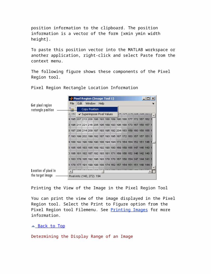
Image Processing Toolbox™
Provide feedback about this page
Resizing an Image
On this page…
Overview
Specifying the Interpolation Method
Preventing Aliasing by Using Filters
Overview
To resize an image, use the imresize function. When you resize an image, you specify the image to be resized and the magnification factor. To enlarge an image, specify a magnification factor greater than 1. To reduce an image, specify a magnification factor between 0 and 1.
. For example, the command below increases the size of an image by 1.25 times.
I = imread('circuit.tif');
J = imresize(I,1.25);
imshow(I)
figure, imshow(J)
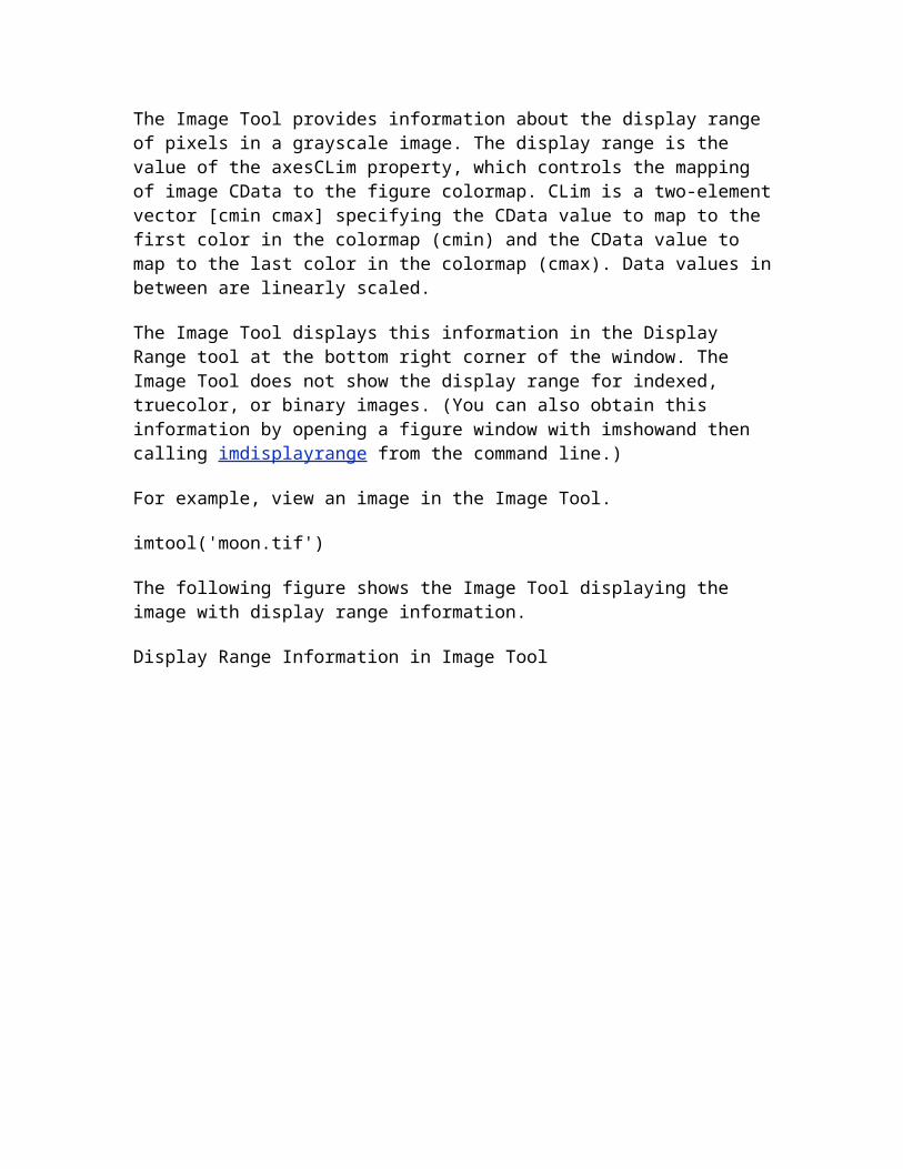
You can specify the size of the output image by passing a vector that contains the number of rows and columns in the output image. If the specified size does not produce the same aspect ratio as the input image, the output image will be distorted. If you specify one of the elements in the vector as NaN, imresize calculates the value for that dimension to preserve the aspect ratio of the image.
This example creates an output image with 100 rows and 150 columns.
I = imread('circuit.tif');
J = imresize(I,[100 150]);
imshow(I)
figure, imshow(J)
To perform the resizing required for multiresolution processing, use the impyramid function.
Back to Top
Specifying the Interpolation Method
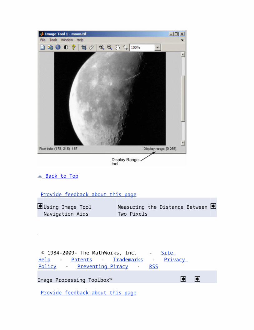
Interpolation is the process used to estimate an image value at a location in between image pixels. When imresize enlarges an image, the output image contains more pixels than the original image. The imresize function uses interpolation to determine the values for the additional pixels.
Interpolation methods determine the value for an interpolated pixel by finding the point in the input image that corresponds to a pixel in the output image and then calculating the value of the output pixel by computing a weighted average of some set of pixels in the vicinity of the point. The weightings are based on the distance each pixel is from the point.
By default, imresize uses bicubic interpolation to determine the values of pixels in the output image, but you can specify other interpolation methods and interpolation kernels. In the following example, imresize uses the bilinear interpolation method. See theimresize reference page for a complete list of interpolation methods and interpolation kernels available. You can also specify your own custom interpolation kernel. .
Y = imresize(X,[100 150],'bilinear')
Back to Top
Preventing Aliasing by Using Filters
When you reduce the size of an image, you lose some of the original pixels because there are fewer pixels in the output image and this can cause aliasing. Aliasing that occurs as a result of size reduction normally appears as "stair-step" patterns (especially in high-contrast images), or as moiré (ripple-effect) patterns in the output image.
By default, imresize uses antialiasing to limit the impact of aliasing on the output image for all interpolation types except nearest neighbor. To turn off antialiasing, specify the 'Antialiasing' parameter and set the value to false.
Note Even with antialiasing, resizing an image can introduce artifacts, because information is always lost when you reduce the size of an image.
For more information, see the reference page for imresize.
Back to Top
Provide feedback about this page
Spatial Transformations Rotating an Image
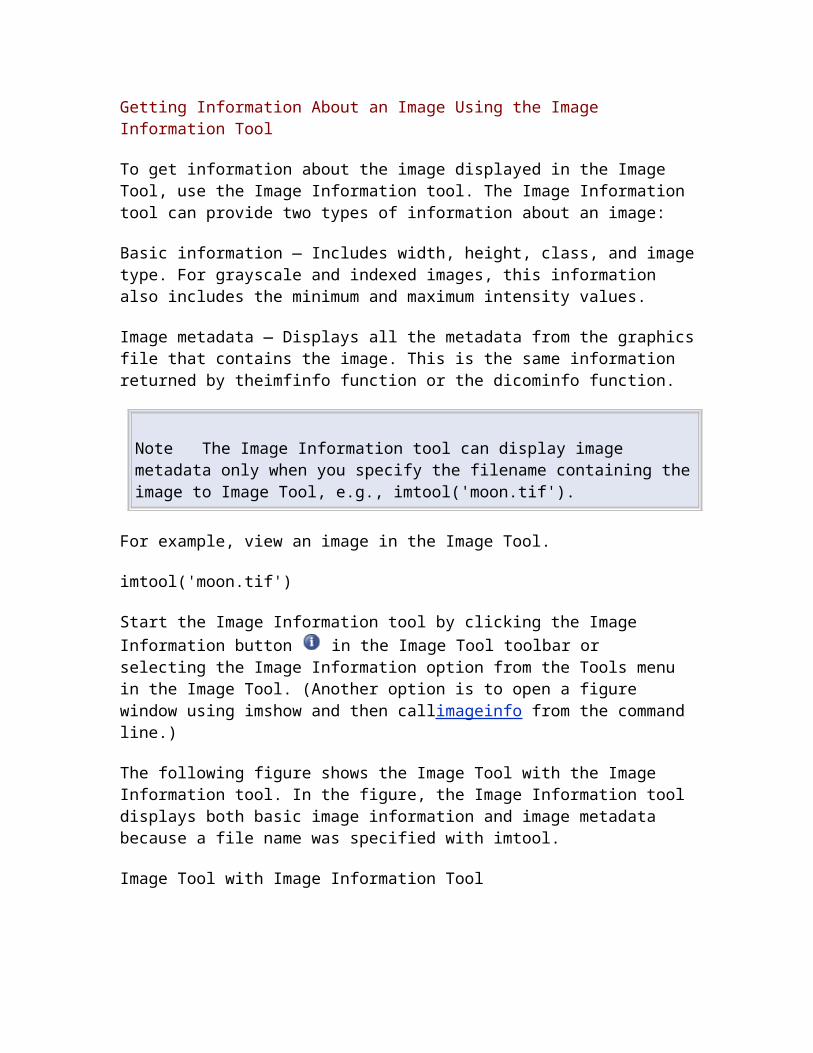
© 1984-2009- The MathWorks, Inc. - Site Help - Patents - Trademarks - Privacy Policy - Preventing Piracy - RSS
Image Processing Toolbox™
Provide feedback about this page
Rotating an Image
To rotate an image, use the imrotate function. When you rotate an image, you specify the image to be rotated and the rotation angle, in degrees. If you specify a positive rotation angle, imrotate rotates the image counterclockwise; if you specify a negative rotation angle,imrotate rotates the image clockwise.
By default, imrotate creates an output image large enough to include the entire original image. Pixels that fall outside the boundaries of the original image are set to 0 and appear as a black background in the output image. You can, however, specify that the output image be the same size as the input image, using the 'crop' argument. Similarly, imrotate uses nearest-neighbor interpolation by default to determine the value of pixels in the output image, but you can specify other interpolation methods. See the imrotate reference page for a list of supported interpolation methods.
This example rotates an image 35° counterclockwise and specifies bilinear interpolation.
I = imread('circuit.tif');
J = imrotate(I,35,'bilinear');
imshow(I)
figure, imshow(J)
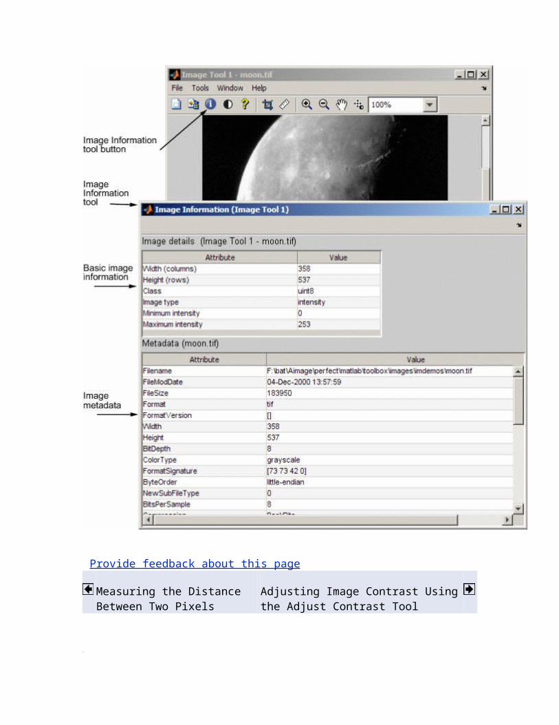
Provide feedback about this page
Resizing an Image Cropping an Image
© 1984-2009- The MathWorks, Inc. - Site Help - Patents - Trademarks - Privacy Policy - Preventing Piracy - RSS
Image Processing Toolbox™
Provide feedback about this page
Cropping an Image
Note You can also crop an image interactively using the Image Tool — see Cropping an Image Using the Crop Image Tool.

To extract a rectangular portion of an image, use the imcrop function. Using imcrop, you can specify the crop region interactively using the mouse or programmatically by specifying the size and position of the crop region.
This example illustrates an interactive syntax. The example reads an image into the MATLAB workspace and calls imcrop specifying the image as an argument. imcrop displays the image in a figure window and waits for you to draw the crop rectangle on the image. When you move the pointer over the image, the shape of the
pointer changes to cross hairs . Click and drag the pointer to specify the size and position of the crop rectangle. You can move and adjust the size of the crop rectangle using the mouse. When you are satisfied with the crop rectangle, double-click to perform the crop operation, or right-click inside the crop rectangle and select Crop Image from the context menu. imcrop returns the cropped image in J.
I = imread('circuit.tif')
J = imcrop(I);
You can also specify the size and position of the crop rectangle as parameters when you call imcrop. Specify the crop rectangle as a four-element position vector, [xmin ymin width height].
In this example, you call imcrop specifying the image to crop, I, and the crop rectangle. imcrop returns the cropped image in J.
I = imread('circuit.tif');
J = imcrop(I,[60 40 100 90]);
Provide feedback about this page
Rotating an Image Performing General 2-D Spatial Transformations
© 1984-2009- The MathWorks, Inc. - Site Help - Patents - Trademarks - Privacy Policy - Preventing Piracy - RSS
Image Processing Toolbox™
Provide feedback about this page
Designing and Implementing 2-D Linear Filters for Image Data
The Image Processing Toolbox software provides a number of functions for designing and implementing two-dimensional linear filters for image data. This chapter describes these functions and how to use them effectively.
Designing and Implementing Linear Filters in the Spatial Domain
Designing Linear Filters in the Frequency Domain
Provide feedback about this page
Using Correlation to Improve Control Points
Designing and Implementing Linear Filters in the Spatial Domain
© 1984-2009- The MathWorks, Inc. - Site Help - Patents - Trademarks - Privacy Policy - Preventing Piracy - RSS
Image Processing Toolbox™

Provide feedback about this page
Removing Noise from Images
On this page…
Understanding Sources of Noise in Digital Images
Removing Noise By Linear Filtering
Removing Noise By Median Filtering
Removing Noise By Adaptive Filtering
Understanding Sources of Noise in Digital Images
Digital images are prone to a variety of types of noise. Noise is the result of errors in the image acquisition process that result in pixel values that do not reflect the true intensities of the real scene. There are several ways that noise can be introduced into an image, depending on how the image is created. For example:
If the image is scanned from a photograph made on film, the film grain is a source of noise. Noise can also be the result of damage to the film, or be introduced by the scanner itself.
If the image is acquired directly in a digital format, the mechanism for gathering the data (such as a CCD detector) can introduce noise.
Electronic transmission of image data can introduce noise.
To simulate the effects of some of the problems listed above, the toolbox provides the imnoise function, which you can use to add various types of noise to an image. The examples in this section use this function.
Back to Top
Removing Noise By Linear Filtering
You can use linear filtering to remove certain types of noise. Certain filters, such as averaging or Gaussian filters, are appropriate for this purpose. For example, an averaging filter is useful for removing grain noise from a photograph. Because each pixel gets set to the average of the pixels in its neighborhood, local variations caused by grain are reduced.

See Designing and Implementing Linear Filters in the Spatial Domain for more information about linear filtering using imfilter.
Back to Top
Removing Noise By Median Filtering
Median filtering is similar to using an averaging filter, in that each output pixel is set to an average of the pixel values in the neighborhood of the corresponding input pixel. However, with median filtering, the value of an output pixel is determined by the median of the neighborhood pixels, rather than the mean. The median is much less sensitive than the mean to extreme values (called outliers). Median filtering is therefore better able to remove these outliers without reducing the sharpness of the image. The medfilt2 function implements median filtering.
Note Median filtering is a specific case of order-statistic filtering, also known as rank filtering. For information about order-statistic filtering, see the reference page for the ordfilt2 function.
The following example compares using an averaging filter and medfilt2 to remove salt and pepper noise. This type of noise consists of random pixels' being set to black or white (the extremes of the data range). In both cases the size of the neighborhood used for filtering is 3-by-3.
Read in the image and display it.
I = imread('eight.tif');
imshow(I)

Add noise to it.
J = imnoise(I,'salt & pepper',0.02);
figure, imshow(J)
Filter the noisy image with an averaging filter and display the results.
K = filter2(fspecial('average',3),J)/255;
figure, imshow(K)
Now use a median filter to filter the noisy image and display the results. Notice that medfilt2 does a better job of removing noise, with less blurring of edges.
L = medfilt2(J,[3 3]);
figure, imshow(L)

Back to Top
Removing Noise By Adaptive Filtering
The wiener2 function applies a Wiener filter (a type of linear filter) to an image adaptively, tailoring itself to the local image variance. Where the variance is large, wiener2 performs little smoothing. Where the variance is small, wiener2 performs more smoothing.
This approach often produces better results than linear filtering. The adaptive filter is more selective than a comparable linear filter, preserving edges and other high-frequency parts of an image. In addition, there are no design tasks; the wiener2 function handles all preliminary computations and implements the filter for an input image. wiener2, however, does require more computation time than linear filtering.
wiener2 works best when the noise is constant-power ("white") additive noise, such as Gaussian noise. The example below applieswiener2 to an image of Saturn that has had Gaussian noise added.
Read in an image. Because the image is a truecolor image, the example converts it to grayscale.
RGB = imread('saturn.png');
I = rgb2gray(RGB);
The example then add Gaussian noise to the image and then displays the image. Because the image is quite large, the figure only shows a portion of the image.
J = imnoise(I,'gaussian',0,0.025);
imshow(J)
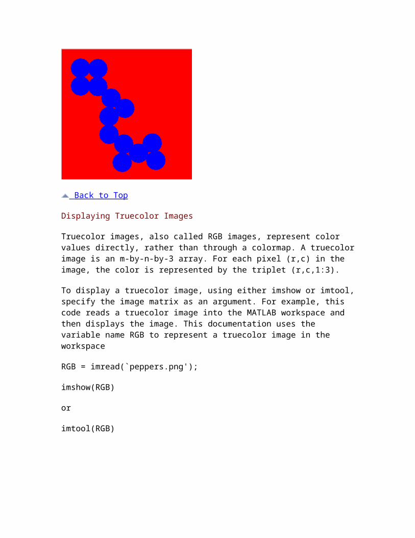
Portion of the Image with Added Gaussian Noise
Remove the noise, using the wiener2 function. Again, the figure only shows a portion of the image
K = wiener2(J,[5 5]);
figure, imshow(K)
Portion of the Image with Noise Removed by Wiener Filter
Back to Top
Provide feedback about this page
Adjusting Pixel Intensity Values ROI-Based Processing
© 1984-2009- The MathWorks, Inc. - Site Help - Patents - Trademarks - Privacy Policy - Preventing Piracy - RSS
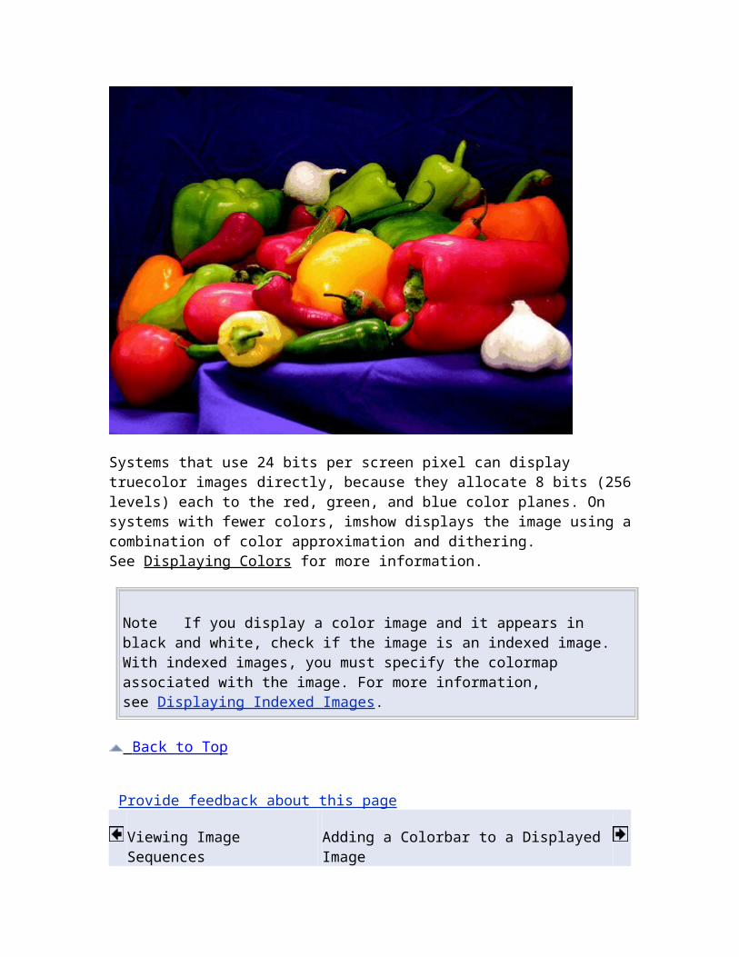
Image Processing Toolbox™
Provide feedback about this page
Function Reference Alphabetical List
Image Display and Exploration Display, import, and export images
GUI Tools Modular interactive tools and associated utility functions.
Spatial Transformation and Image Registration
Spatial transformation and image registration
Image Analysis and Statistics Image analysis, texture analysis, view pixel values, and calculate image statistics
Image Arithmetic Add, subtract, multiply, and divide images
Image Enhancement and Restoration Enhance and restore images
Linear Filtering and Transforms Linear filters, filter design, and image transforms
Morphological Operations Morphological image processing
ROI-Based, Neighborhood, and Block Processing
ROI-based, neighborhood, and block operations
Colormaps and Color Space Manipulate image color
Utilities Array operations, demos, preferences and other toolbox utility functions
Back to Top
Image Display and Exploration
Image Display and Exploration Display and explore images
Image File I/O Import and export images
Image Types and Type Conversions Convert between the various image types
Back to Top of Section
Image Display and Exploration
immovie Make movie from multiframe image
implay Play movies, videos, or image sequences
imshow Display image
imtool Image Tool
montage Display multiple image frames as rectangular montage
subimage Display multiple images in single figure
warp Display image as texture-mapped surface
Back to Top of Section
Image File I/O
analyze75info Read metadata from header file of Analyze 7.5 data set
analyze75read Read image data from image file of Analyze 7.5 data set
dicomanon Anonymize DICOM file

dicomdict Get or set active DICOM data dictionary
dicominfo Read metadata from DICOM message
dicomlookup Find attribute in DICOM data dictionary
dicomread Read DICOM image
dicomuid Generate DICOM unique identifier
dicomwrite Write images as DICOM files
hdrread Read high dynamic range (HDR) image
hdrwrite Write Radiance high dynamic range (HDR) image file
interfileinfo Read metadata from Interfile file
interfileread Read images in Interfile format
isrset Check if file is an R-Set
makehdr Create high dynamic range image
nitfinfo Read metadata from National Imagery Transmission Format (NITF) file
nitfread Read image from NITF file
rsetwrite Create reduced resolution data set from image file
tonemap Render high dynamic range image for viewing
Back to Top of Section
Image Types and Type Conversions
demosaic Convert Bayer pattern encoded image to truecolor image
gray2ind Convert grayscale or binary image to indexed image

grayslice Convert grayscale image to indexed image using multilevel thresholding
graythresh Global image threshold using Otsu's method
im2bw Convert image to binary image, based on threshold
im2double Convert image to double precision
im2int16 Convert image to 16-bit signed integers
im2java2d Convert image to Java buffered image
im2single Convert image to single precision
im2uint16 Convert image to 16-bit unsigned integers
im2uint8 Convert image to 8-bit unsigned integers
ind2gray Convert indexed image to grayscale image
ind2rgb Convert indexed image to RGB image
label2rgb Convert label matrix into RGB image
mat2gray Convert matrix to grayscale image
rgb2gray Convert RGB image or colormap to grayscale
Back to Top
GUI Tools
Modular Interactive Tools Modular interactive tool creation functions
Navigational Tools for Image Scroll Panel Modular interactive navigational tools
Utilities for Interactive Tools Modular interactive tool utility functions

Back to Top of Section
Modular Interactive Tools
imageinfo Image Information tool
imcontrast Adjust Contrast tool
imdisplayrange Display Range tool
imdistline Distance tool
impixelinfo Pixel Information tool
impixelinfoval Pixel Information tool without text label
impixelregion Pixel Region tool
impixelregionpanel Pixel Region tool panel
Back to Top of Section
Navigational Tools for Image Scroll Panel
immagbox Magnification box for scroll panel
imoverview Overview tool for image displayed in scroll panel
imoverviewpanel Overview tool panel for image displayed in scroll panel
imscrollpanel Scroll panel for interactive image navigation
Back to Top of Section
Utilities for Interactive Tools
axes2pix Convert axes coordinates to pixel coordinates
getimage Image data from axes
getimagemodel Image model object from image object
imattributes Information about image attributes
imellipse Create draggable ellipse
imfreehand Create draggable freehand region
imgca Get handle to current axes containing image
imgcf Get handle to current figure containing image
imgetfile Open Image dialog box
imhandles Get all image handles
imline Create draggable, resizable line
impoint Create draggable point
impoly Create draggable, resizable polygon
imrect Create draggable rectangle
imroi Region-of-interest (ROI) base class
iptaddcallback Add function handle to callback list
iptcheckhandle Check validity of handle
iptgetapi Get Application Programmer Interface (API) for handle
iptGetPointerBehavior Retrieve pointer behavior from HG object
ipticondir Directories containing IPT and MATLAB icons
iptPointerManager Create pointer manager in figure
iptremovecallback Delete function handle from callback list
iptSetPointerBehavior Store pointer behavior structure in Handle Graphics object

iptwindowalign Align figure windows
makeConstrainToRectFcn
Create rectangularly bounded drag constraint function
truesize Adjust display size of image
Back to Top
Spatial Transformation and Image Registration
Spatial Transformations Spatial transformation of images and multidimensional arrays
Image Registration Align two images using control points
Back to Top of Section
Spatial Transformations
checkerboard Create checkerboard image
findbounds Find output bounds for spatial transformation
fliptform Flip input and output roles of TFORM structure
imcrop Crop image
impyramid Image pyramid reduction and expansion
imresize Resize image
imrotate Rotate image
imtransform Apply 2-D spatial transformation to image
makeresampler Create resampling structure
maketform Create spatial transformation structure (TFORM)

tformarray Apply spatial transformation to N-D array
tformfwd Apply forward spatial transformation
tforminv Apply inverse spatial transformation
Back to Top of Section
Image Registration
cp2tform Infer spatial transformation from control point pairs
cpcorr Tune control-point locations using cross correlation
cpselect Control Point Selection Tool
cpstruct2pairs Convert CPSTRUCT to valid pairs of control points
normxcorr2 Normalized 2-D cross-correlation
Back to Top
Image Analysis and Statistics
Image Analysis Trace boundaries, detect edges, and perform quadtree decomposition
Texture Analysis Entropy, range, and standard deviation filtering; gray-level co-occurrence matrix
Pixel Values and Statistics Create histograms, contour plots, and get statistics on image regions
Back to Top of Section
Image Analysis
bwboundaries Trace region boundaries in binary image
bwtraceboundary Trace object in binary image
cornermetric Create corner metric matrix from image
edge Find edges in grayscale image
hough Hough transform
houghlines Extract line segments based on Hough transform
houghpeaks Identify peaks in Hough transform
qtdecomp Quadtree decomposition
qtgetblk Block values in quadtree decomposition
qtsetblk Set block values in quadtree decomposition
Back to Top of Section
Texture Analysis
entropy Entropy of grayscale image
entropyfilt Local entropy of grayscale image
graycomatrix Create gray-level co-occurrence matrix from image
graycoprops Properties of gray-level co-occurrence matrix
rangefilt Local range of image
stdfilt Local standard deviation of image
Back to Top of Section
Pixel Values and Statistics

corr2 2-D correlation coefficient
imcontour Create contour plot of image data
imhist Display histogram of image data
impixel Pixel color values
improfile Pixel-value cross-sections along line segments
mean2 Average or mean of matrix elements
regionprops Measure properties of image regions
std2 Standard deviation of matrix elements
Back to Top
Image Arithmetic
imabsdiff Absolute difference of two images
imadd Add two images or add constant to image
imcomplement Complement image
imdivide Divide one image into another or divide image by constant
imlincomb Linear combination of images
immultiply Multiply two images or multiply image by constant
imsubtract Subtract one image from another or subtract constant from image
Back to Top
Image Enhancement and Restoration
Image Enhancement Histogram equalization, decorrelation

stretching, and 2-D filtering
Image Restoration (Deblurring) Deconvolution for deblurring
Back to Top of Section
Image Enhancement
adapthisteq Contrast-limited adaptive histogram equalization (CLAHE)
decorrstretch Apply decorrelation stretch to multichannel image
histeq Enhance contrast using histogram equalization
imadjust Adjust image intensity values or colormap
imnoise Add noise to image
intlut Convert integer values using lookup table
medfilt2 2-D median filtering
ordfilt2 2-D order-statistic filtering
stretchlim Find limits to contrast stretch image
wiener2 2-D adaptive noise-removal filtering
Back to Top of Section
Image Restoration (Deblurring)
deconvblind Deblur image using blind deconvolution
deconvlucy Deblur image using Lucy-Richardson method
deconvreg Deblur image using regularized filter

deconvwnr Deblur image using Wiener filter
edgetaper Taper discontinuities along image edges
otf2psf Convert optical transfer function to point-spread function
psf2otf Convert point-spread function to optical transfer function
Back to Top
Linear Filtering and Transforms
Linear Filtering Convolution, N-D filtering, and predefined 2-D filters
Linear 2-D Filter Design 2-D FIR filters
Image Transforms Fourier, Discrete Cosine, Radon, and Fan-beam transforms
Back to Top of Section
Linear Filtering
convmtx2 2-D convolution matrix
fspecial Create predefined 2-D filter
imfilter N-D filtering of multidimensional images
Back to Top of Section
Linear 2-D Filter Design
freqz2 2-D frequency response
fsamp2 2-D FIR filter using frequency sampling
ftrans2 2-D FIR filter using frequency transformation
fwind1 2-D FIR filter using 1-D window method
fwind2 2-D FIR filter using 2-D window method
Back to Top of Section
Image Transforms
dct2 2-D discrete cosine transform
dctmtx Discrete cosine transform matrix
fan2para Convert fan-beam projections to parallel-beam
fanbeam Fan-beam transform
idct2 2-D inverse discrete cosine transform
ifanbeam Inverse fan-beam transform
iradon Inverse Radon transform
para2fan Convert parallel-beam projections to fan-beam
phantom Create head phantom image
radon Radon transform
Back to Top
Morphological Operations
Intensity and Binary Images Dilate, erode, reconstruct, and perform other morphological operations
Binary Images Label, pack, and perform morphological operations on binary images

Structuring Element Creation and Manipulation
Create and manipulate structuring elements for morphological operations
Back to Top of Section
Intensity and Binary Images
conndef Create connectivity array
imbothat Bottom-hat filtering
imclearborder Suppress light structures connected to image border
imclose Morphologically close image
imdilate Dilate image
imerode Erode image
imextendedmax Extended-maxima transform
imextendedmin Extended-minima transform
imfill Fill image regions and holes
imhmax H-maxima transform
imhmin H-minima transform
imimposemin Impose minima
imopen Morphologically open image
imreconstruct Morphological reconstruction
imregionalmax Regional maxima
imregionalmin Regional minima

imtophat Top-hat filtering
watershed Watershed transform
Back to Top of Section
Binary Images
applylut Neighborhood operations on binary images using lookup tables
bwarea Area of objects in binary image
bwareaopen Morphologically open binary image (remove small objects)
bwdist Distance transform of binary image
bweuler Euler number of binary image
bwhitmiss Binary hit-miss operation
bwlabel Label connected components in 2-D binary image
bwlabeln Label connected components in binary image
bwmorph Morphological operations on binary images
bwpack Pack binary image
bwperim Find perimeter of objects in binary image
bwselect Select objects in binary image
bwulterode Ultimate erosion
bwunpack Unpack binary image
imregionalmin Regional minima
imtophat Top-hat filtering

makelut Create lookup table for use with applylut
Back to Top of Section
Structuring Element Creation and Manipulation
getheight Height of structuring element
getneighbors Structuring element neighbor locations and heights
getnhood Structuring element neighborhood
getsequence Sequence of decomposed structuring elements
isflat True for flat structuring element
reflect Reflect structuring element
strel Create morphological structuring element (STREL)
translate Translate structuring element (STREL)
Back to Top
ROI-Based, Neighborhood, and Block Processing
ROI-Based Processing Define regions of interest (ROI) and perform operations on them
Neighborhood and Block Processing Define neighborhoods and blocks and process them
Back to Top of Section
ROI-Based Processing
poly2mask Convert region of interest (ROI) polygon to region mask

roicolor Select region of interest (ROI) based on color
roifill Fill in specified region of interest (ROI) polygon in grayscale image
roifilt2 Filter region of interest (ROI) in image
roipoly Specify polygonal region of interest (ROI)
Back to Top of Section
Neighborhood and Block Processing
bestblk Determine optimal block size for block processing
blkproc Distinct block processing for image
col2im Rearrange matrix columns into blocks
colfilt Columnwise neighborhood operations
im2col Rearrange image blocks into columns
nlfilter General sliding-neighborhood operations
Back to Top
Colormaps and Color Space
Color Space Conversions ICC profile-based device independent color space conversions and device-dependent color space conversions
Back to Top of Section
Color Space Conversions
applycform Apply device-independent color space transformation
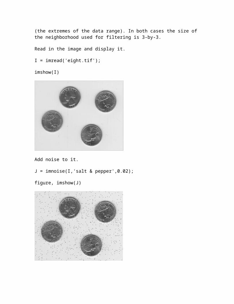
iccfind Search for ICC profiles
iccread Read ICC profile
iccroot Find system default ICC profile repository
iccwrite Write ICC color profile to disk file
isicc True for valid ICC color profile
lab2double Convert L*a*b* data to double
lab2uint16 Convert L*a*b* data to uint16
lab2uint8 Convert L*a*b* data to uint8
makecform Create color transformation structure
ntsc2rgb Convert NTSC values to RGB color space
rgb2ntsc Convert RGB color values to NTSC color space
rgb2ycbcr Convert RGB color values to YCbCr color space
whitepoint XYZ color values of standard illuminants
xyz2double Convert XYZ color values to double
xyz2uint16 Convert XYZ color values to uint16
ycbcr2rgb Convert YCbCr color values to RGB color space
Back to Top
Utilities
Preferences Set and determine value of toolbox preferences
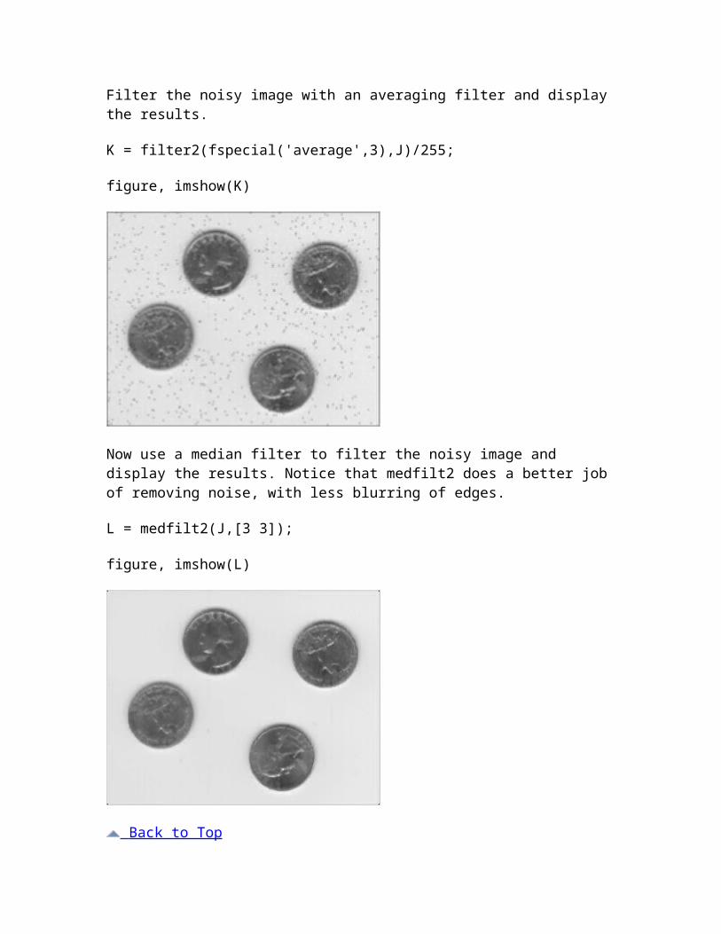
Validation Check input arguments and perform other common programming tasks
Mouse Retrieve values of lines, points, and rectangles defined interactively using mouse
Array Operations Circularly shift pixel values and pad arrays
Demos Launch Image Processing Toolbox demos
Performance Check for presence of Intel Integrated Performance Primitives (Intel IPP) library
Back to Top of Section
Preferences
iptgetpref Get values of Image Processing Toolbox preferences
iptprefs Opens Image Processing Preferences dialog box
iptsetpref Set Image Processing Toolbox preferences or display valid values
Back to Top of Section
Validation
getrangefromclass Default display range of image based on its class
iptcheckconn Check validity of connectivity argument
iptcheckinput Check validity of array
iptcheckmap Check validity of colormap

iptchecknargin Check number of input arguments
iptcheckstrs Check validity of option string
iptnum2ordinal Convert positive integer to ordinal string
Back to Top of Section
Mouse
getline Select polyline with mouse
getpts Specify points with mouse
getrect Specify rectangle with mouse
Back to Top of Section
Array Operations
padarray Pad array
Back to Top of Section
Demos
iptdemos Index of Image Processing Toolbox demos
Functions — Alphabetical List By Category
A B C D E F G H I J K L M N O P Q R S T U V W X Y Z
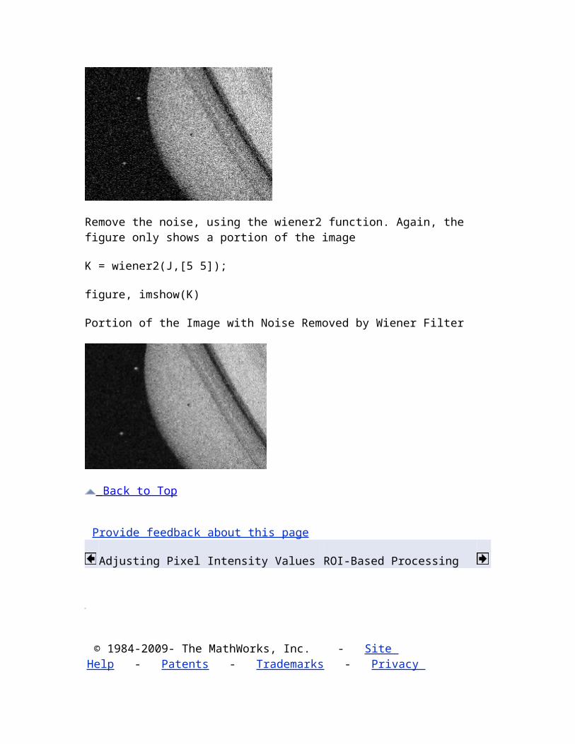
adapthisteqanalyze75infoanalyze75readapplycformapplylutaxes2pixbestblk blkprocbwareabwareaopenbwboundariesbwconncompbwdistbweulerbwhitmissbwlabelbwlabelnbwmorphbwpackbwperimbwselectbwtraceboundarybwulterodebwunpackcheckerboard col2imcolfiltconndefconvmtx2cornermetriccorr2cp2tformcpcorrcpselectcpstruct2pairsdct2 dctmtxdeconvblinddeconvlucydeconvregdeconvwnrdecorrstretchdemosaicdicomanondicomdictdicominfo
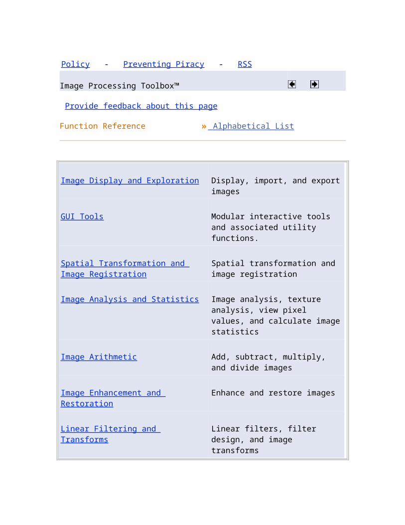
dicomlookupdicomreaddicomuiddicomwriteedge edgetaperentropyentropyfiltfan2para fanbeamfindboundsfliptformfreqz2fsamp2fspecialftrans2fwind1fwind2getheight getimagegetimagemodelgetlinegetneighborsgetnhoodgetptsgetrangefromclassgetrectgetsequencegray2indgraycomatrixgraycopropsgrayslicegraythreshhdrread hdrwritehisteqhoughhoughlineshoughpeaksiccfind iccreadiccrooticcwriteidct2ifanbeamim2bw
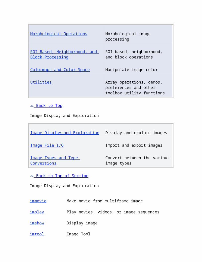
im2colim2doubleim2int16im2java2dim2singleim2uint16im2uint8imabsdiffimaddimadjustimageinfoimagemodelimattributesimbothatimclearborderimcloseimcolormaptoolimcomplementimcontourimcontrastimcropimdilateimdisplayrangeimdistlineimdivideimellipseimerodeimextendedmaximextendedminimfillimfilterimfreehandimgcaimgcfimgetfileimhandlesimhistimhmaximhminimimposeminimlincombimlineimmagboximmovieimmultiplyimnoise

imopenimoverviewimoverviewpanelimpixelimpixelinfoimpixelinfovalimpixelregionimpixelregionpanelimplayimpointimpolyimpositionrectimprofileimputfileimpyramidimreconstructimrectimregionalmaximregionalminimresizeimroiimrotateimsaveimscrollpanelimshowimsubtractimtoolimtophatimtransformimviewind2grayind2rgbinterfileinfointerfilereadintlutippliptaddcallbackiptcheckconniptcheckhandleiptcheckinputiptcheckmapiptchecknarginiptcheckstrsiptdemosiptgetapiiptGetPointerBehavior

iptgetprefipticondiriptnum2ordinaliptPointerManageriptprefsiptremovecallbackiptSetPointerBehavioriptsetprefiptwindowaligniradonisbwisflatisgrayisiccisindisnitfisrgbisrsetlab2double lab2uint16lab2uint8label2rgblabelmatrixmakecform makeConstrainToRectFcnmakehdrmakelutmakeresamplermaketformmat2graymean2medfilt2montagenitfinfo nitfreadnlfilternormxcorr2ntsc2rgbordfilt2 otf2psfpadarray para2fanphantompoly2maskpsf2otfqtdecomp
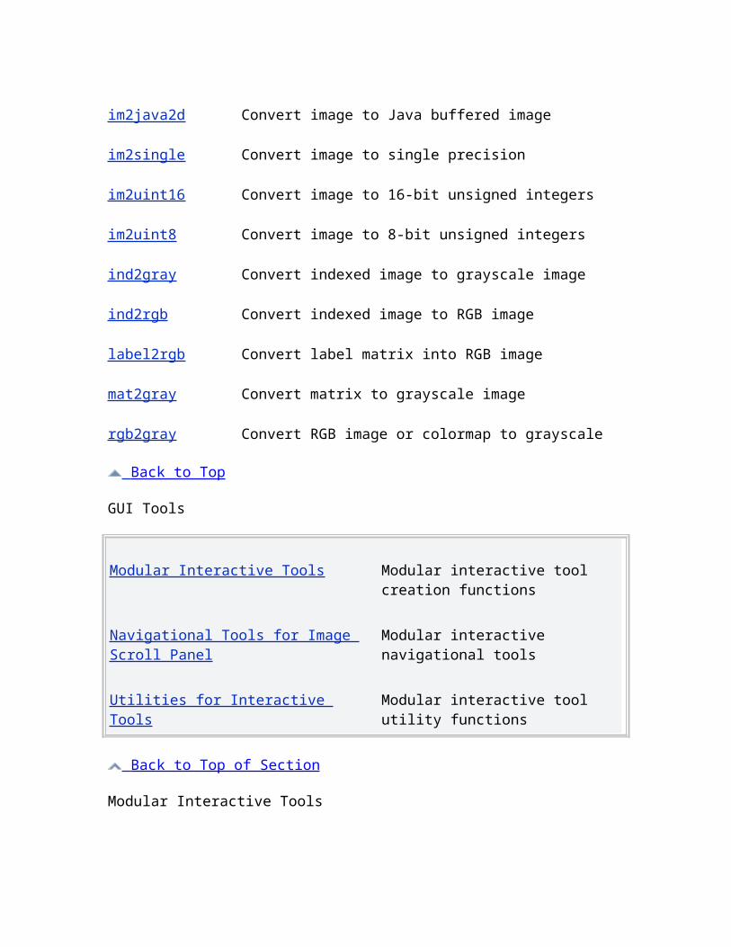
qtgetblkqtsetblkradon rangefiltreflectregionpropsrgb2grayrgb2ntscrgb2ycbcrroicolorroifillroifilt2roipolyrsetwritestd2 stdfiltstrelstretchlimsubimagetformarray tformfwdtforminvtonemaptranslatetruesizeuintlut warp watershedwhitepointwiener2xyz2double xyz2uint16ycbcr2rgb