Image Transformations and Blurring

Image Transformations and BlurringJustin Domke and Yiannis Aloimonos

Abstract—Since cameras blur the incoming light during measurement, different images of the same surface do not contain the same

information about that surface. Thus, in general, corresponding points in multiple views of a scene have different image intensities.

While multiple-view geometry constrains the locations of corresponding points, it does not give relationships between the signals at

corresponding locations. This paper offers an elementary treatment of these relationships. We first develop the notion of “ideal” and

“real” images, corresponding to, respectively, the raw incoming light and the measured signal. This framework separates the filtering

and geometric aspects of imaging. We then consider how to synthesize one view of a surface from another; if the transformation

between the two views is affine, it emerges that this is possible if and only if the singular values of the affine matrix are positive. Next,

we consider how to combine the information in several views of a surface into a single output image. By developing a new tool called

“frequency segmentation,” we show how this can be done despite not knowing the blurring kernel.

Index Terms—Reconstruction, restoration, sharpening and deblurring, smoothing.

Ç

1 INTRODUCTION

THIS paper concerns a very basic question: what are therelationships between multiple views of a surface? This

question is only partially answered by the geometry of thesituation. Consider two points in different images that projectto the same 3D surface point. Even supposing that the imagesare perfectly Lambertian and disregarding issues like lightingor noise, the image intensities will still in general be different.This is because cameras do not merely measure the incominglight. During measurement, the signal is optically filtered orblurred. Given the finite resolution of cameras, this isnecessary to avoid aliasing effects. However, because thisblurring is fixed to the camera’s coordinate system, differentviews of a surface result in different measured signals. This istrue even after correcting for the geometrical transformationbetween the views.

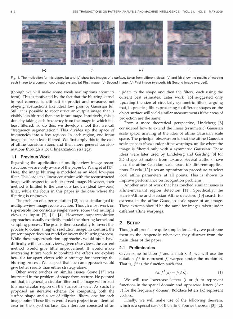
Fig. 1 shows an example of two images of a surface andthe results of warping them to a common coordinatesystem. To understand this situation, this paper introducesa simple formalism. We contrast between what we call the“ideal image,” corresponding to the unblurred incominglight, and the “real image,” corresponding to the measuredsignal. The ideal image cannot be measured but is useful foranalysis because it is immune to blurring. If the ideal imageis some function i and the real image is some function j, wewrite j ¼ i � e, where e is the blurring kernel. (Here, i, j, ande are all continuous functions. Assuming that the signal islow-pass filtered appropriately, j can be reconstructed fromthe discretely sampled pixels.) The advantage of this is thatgiven the transformation between two views, one view’sideal image exactly specifies the other’s. Notice that the

3D structure of the scene does not need to be explicitlyconsidered, only the resulting transformation of surfacesbetween different views.

Given this setup, it is easy to derive a number of theoremsabout the relationships between different views. After a fewbasic results, we will ask the following question: Suppose thereal image j2 for a view is known, as well as the blurringkernel e. Suppose also that the transformation between theviews is affine: x1 in the first view corresponds to x2 in thesecond view if and only if x2 ¼ Ax1, whereA is a 2� 2 matrix.(It is convenient to ignore translation, since this does notimpact the blurring kernel.) When will it be possible toconstruct the (real) image for the first view, without invertingthe blurring kernel? Our first main result is that this ispossible if and only if the singular values ofA are greater thanone. This is true independently of e, as long as it is a circularlysymmetric low-pass filter. This theorem reduces to knownresults for the special case of Gaussian blurring.

Next, we briefly discuss possible applications of theabove theorem to image matching for widely separatedviews. Suppose that two patches are given and one wants tocheck if they might match under some affine motion A.There are three cases of interest. First, if the singular valuesof A are greater than one, the above theorem applies: Oneimage can be filtered as above so as to remove anyinformation that is not present in the other image. Afterfiltering, if the images do match, they should be the same.The second case, where the singular values of A are bothless than one, can be handled in a similar way. However, ifone singular value is greater than one and one is less, thesituation is more complex. Nevertheless, we derive filtersthat will remove the least amount of information, whilemaking it possible to compare the patches.

Finally, as an example of the practical use of thisframework, we consider the problem of multiple-viewimage reconstruction. Suppose that we have several views,as well as the transformations between them. Now, wewant to construct an output image containing the bestcontent from all input images. Here, we consider thisproblem in the context that the blurring kernel e is unknown

IEEE TRANSACTIONS ON PATTERN ANALYSIS AND MACHINE INTELLIGENCE, VOL. 31, NO. 5, MAY 2009 811

. The authors are with the Center for Automation Research, University ofMaryland, College Park, MD 20742.E-mail: [email protected], [email protected].

Manuscript received 9 Jan. 2008; accepted 5 May 2008; published online 20May 2008.Recommended for acceptance by J. Luo.For information on obtaining reprints of this article, please send e-mail to:[email protected], and reference IEEECS Log NumberTPAMI-2008-01-0017.Digital Object Identifier no. 10.1109/TPAMI.2008.133.

0162-8828/09/$25.00 � 2009 IEEE Published by the IEEE Computer Society

(though we will make some weak assumptions about itsform). This is motivated by the fact that the blurring kernelin real cameras is difficult to predict and measure, notobeying abstractions like ideal low pass or Gaussian [6].Still, it is possible to reconstruct an output image that isvisibly less blurred than any input image. Intuitively, this isdone by taking each frequency from the image in which it isleast filtered. To do this, we develop a tool that we call“frequency segmentation.” This divides up the space offrequencies into a few regions. In each region, one inputimage has been least filtered. We first apply this to the caseof affine transformations and then more general transfor-mations through a local linearization strategy.

1.1 Previous Work

Regarding the application of multiple-view image recon-struction, we are only aware of the paper by Wang et al [17].Here, the image blurring is modeled as an ideal low-passfilter. This leads to a linear constraint with the reconstructedimage with respect to each observed image. However, theirmethod is limited to the case of a known (ideal low-pass)filter, while the focus in this paper is the case where thefiltering is unknown.

The problem of superresolution [12] has a similar goal tomultiple-view image reconstruction. Though most work onsuperresolution considers single views, some take multipleviews as input [7], [1], [4]. However, superresolutionapproaches usually explicitly model the blurring kernel andsampling process. The goal is then essentially to invert thisprocess to obtain a higher resolution image. In contrast, thepresent paper does not model or invert the blurring process.While these superresolution approaches would often havedifficulty with far-apart views, given close views, the currentmethod would give little improvement. It would makeinteresting future work to combine the effects we explorehere for far-apart views with a strategy for inverting theblurring process. We suspect that such an approach wouldgive better results than either strategy alone.

Other work touches on similar issues. Stone [15] wasinterested in the problem of shape from texture. He pointedout that, in general, a circular filter on the image will projectto a noncircular region on the surface in view. As such, heproposed an iterative scheme for computing both thesurface shape and a set of elliptical filters, one for eachimage point. These filters would each project to an identicalarea on the object surface. Each iteration consisted of an

update to the shape and then the filters, each using the

current best estimates. Later work [16] suggested only

updating the size of circularly symmetric filters, arguing

that, in practice, filters projecting to different shapes on the

object surface will yield similar measurements if the areas of

projection are the same.From a more theoretical perspective, Lindeberg [8]

considered how to extend the linear (symmetric) Gaussian

scale space, arriving at the idea of affine Gaussian scale

space. The principal observation is that the affine Gaussian

scale space is closed under affine warpings, unlike where the

image is filtered only with a symmetric Gaussian. These

ideas were later used by Lindeberg and Garding [8] for

3D shape estimation from texture. Several authors have

used the affine Gaussian scale space for different applica-

tions. Ravela [13] uses an optimization procedure to select

local affine parameters at all points. This is shown to

improve performance on recognition problems.Another area of work that has touched similar issues is

affine-invariant region detection [11]. Specifically, the

Harris-Affine and Hessian Affine detectors [10] search for

extrema in the affine Gaussian scale space of an image.

These extrema should be the same for images taken under

different affine warpings.

2 SETUP

Though all proofs are quite simple, for clarity, we postpone

them to the Appendix whenever they distract from the

main ideas of the paper.

2.1 Preliminaries

Given some function f and a matrix A, we will use the

notation fA to represent f , warped under the motion A.

That is, fA is the function such that

8x; fAðxÞ ¼ fðAxÞ: ð1Þ

We will use lowercase letters (i or j) to represent

functions in the spatial domain and uppercase letters (I or

J) for the frequency domain. Boldface letters ðxÞ represent

vectors.Finally, we will make use of the following theorem,

which is a special case of the affine Fourier theorem [3], [2].

812 IEEE TRANSACTIONS ON PATTERN ANALYSIS AND MACHINE INTELLIGENCE, VOL. 31, NO. 5, MAY 2009

Fig. 1. The motivation for this paper. (a) and (b) show two images of a surface, taken from different views. (c) and (d) show the results of warping

each image to a common coordinate system. (a) First image. (b) Second image. (c) First image (warped). (d) Second image (warped).

Theorem 1 (Translation-Free Affine Fourier Theorem). IfFffðxÞg ¼ F ðuÞ, then FffAðxÞg ¼ jA�1jFA�T ðuÞ, whereFð�Þ denotes the Fourier transform.

Proof. (Postponed) tu

2.2 Basic Results

Assume that we have two images of the same surface, takenunder an affine motion. Without loss of generality, assumethat the transformation sends the origin to the origin. Then, ifi1 and i2 are the ideal images, there exists some A such that

x2 ¼ Ax1 ! i2ðx2Þ ¼ i1ðx1Þ; ð2Þ

or, equivalently,

iA2 ðxÞ ¼ i1ðxÞ: ð3Þ

Here, x1 and x2 are 2D vectors and A is a 2 � 2 matrix.Equation (3) makes several simplifying assumptions.

First, it does not model issues such as sensor noise. Second,if the images are taken of a static scene from differentcamera positions, this equation assumes Lambertian reflec-tance. Nevertheless, (3) is sufficient to study the changes tothe signals introduced by camera blurring.

Let j1 and j2 be the real observed images. If e is the low-pass filter applied by the optics of the camera, the realimage is, by definition, the result of convolving the idealimage with e:

j1ðxÞ ¼ ½i1 � e�ðxÞ; ð4Þ

j2ðxÞ ¼ ½i2 � e�ðxÞ: ð5Þ

The results in this paper are independent of theparticular form of e. However, we make two assumptions:

1. e is circularly symmetric. Formally, eðxÞ is a functionof jxj only. Notice that if EðuÞ is the Fouriertransform of eðxÞ, this also implies that E iscircularly symmetric.

2. e is a monotonically decreasing low-pass filter.Formally, if ju2j � ju1j, then Eðu2Þ � Eðu1Þ. (It iseasy to show that E will be real, since eðxÞ ¼ eð�xÞ.)

While these assumptions are close enough to give usefulresults, we note that real cameras do not have perfectlycircularly symmetric blurring, nor do they exactly obey theassumption of translation invariance.

Notice that unlike the ideal images, the real images neednot match at corresponding points:

x2 ¼ Ax1 6! j2ðx2Þ ¼ j1ðx1Þ: ð6Þ

The key result driving this paper is the following.Contrast this with (3) for the ideal images.

Theorem 2 (Affine Blurring Theorem).

jA2 ðxÞ ¼ jAj i1 � eA� �

ðxÞ: ð7Þ


When warped into the coordinate system of the firstimage, the second image is equivalent to the first ideal

image, convolved with a warped version of the low-pass

filter. jAj acts as a normalization factor so that eA integrates

to the same value as e.Another useful result is given by taking the Fourier

transform of both sides of (7).

Theorem 3 (Fourier Affine Blurring Theorem).

FfjA2 ðxÞg ¼ ½I1 � EA�T �ðuÞ: ð8Þ


2.3 Affine Gaussian Scale Space

As an example, suppose the blurring kernel is a Gaussian.

Equation (7) can be used to get the relationship between j1

and jA2 more explicitly. Let N � denote an origin-centered

Gaussian with covariance matrix �. Then, e ¼ N �I :

j1ðxÞ ¼ ½i1 � N �I �ðxÞ: ð9Þ

The following lemma specifies how a Gaussian behaves

under affine warping. (This result follows easily by

substituting Ax in place of x in the definition of a

Gaussian.)

Lemma 1.

N A�ðxÞ ¼

1

jAj N A�1�A�T ðxÞ: ð10Þ

From this, the following relationship follows immediately:

jA2 ðxÞ ¼ ½i1 � N �A�1A�T �ðxÞ: ð11Þ

Notice that the constant of jAj was absorbed into the

Gaussian. Essentially, this same relationship is known in

the literature on affine Gaussian scale space [9].

2.4 Parameterization of A

Though A has four parameters, it turns out that there are

only three parameters of interest to us here. Consider the

following decomposition of A [5]:

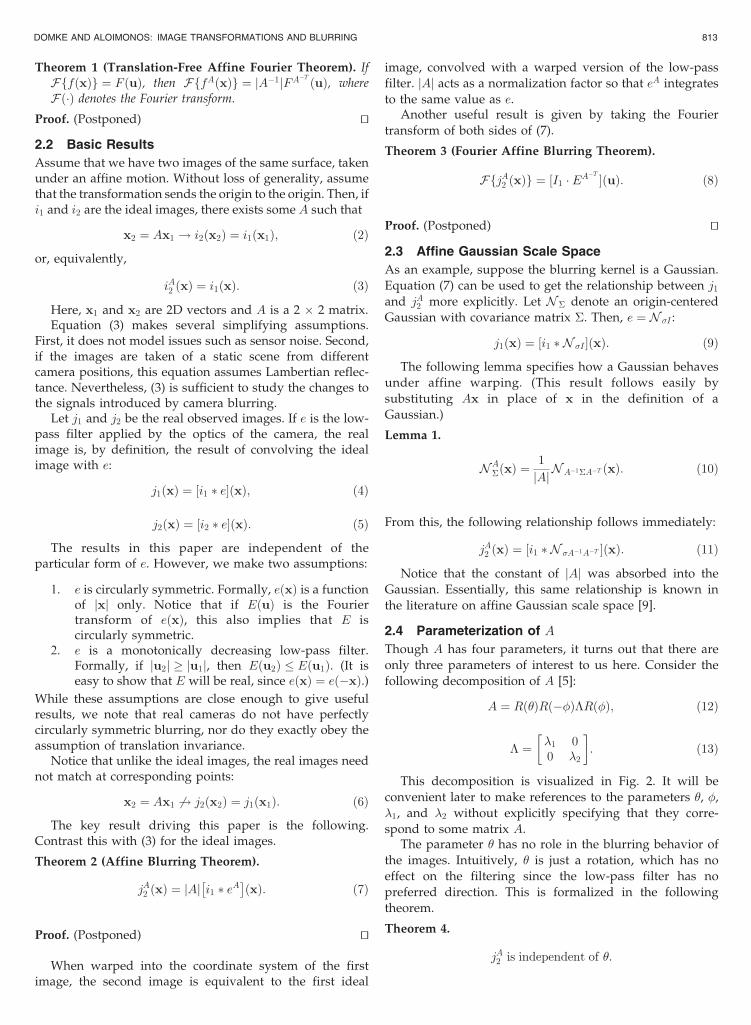
A ¼ Rð�ÞRð��Þ�Rð�Þ; ð12Þ

� ¼ �1 00 �2

� �: ð13Þ

This decomposition is visualized in Fig. 2. It will be

convenient later to make references to the parameters �, �,

�1, and �2 without explicitly specifying that they corre-

spond to some matrix A.The parameter � has no role in the blurring behavior of

the images. Intuitively, � is just a rotation, which has no

effect on the filtering since the low-pass filter has no

preferred direction. This is formalized in the following

theorem.

Theorem 4.

jA2 is independent of �:

DOMKE AND ALOIMONOS: IMAGE TRANSFORMATIONS AND BLURRING 813

Proof. Notice that the expression for j2 in (7) dependson A only through jAj and eA. By our assumption

that e is circularly symmetric, eAðxÞ ¼ eðAxÞ ¼eðjAxjÞ ¼ eðj�Rð�ÞxjÞ does not depend on �. It is alsoeasy to see that jAj is independent of �. tu

3 TWO-VIEW ACCESSIBILITY

Suppose we are given only A and j2. A question arises: Is itpossible to filter jA2 so as to synthesize j1? As we will showbelow, this is only possible sometimes.

In this paper, we want to avoid the problem of

deconvolution or deblurring. In theory, if the low-passfilter E was nonzero for all frequencies, it would be possibleto increase the magnitude of all frequencies to completely

cancel out the effects of the filtering. With the ideal image inhand, any other view could be synthesized. However, inpractice, this can be done only for a limited range offrequencies because, for high frequencies, the noise in the

observed image will usually be much larger than the signalremaining after filtering [14]. If deconvolution is practical,we can imagine that it has already been applied and the

problem restated with an appropriately changed blurringkernel and input images. Hence, we will not attempt toinvert the blurring kernel.

Suppose that we apply some filter d to one of the images.

If D is the Fourier transform of d, we require that D does notincrease the magnitude of any frequency. Formally, for allu, we must have DðuÞ � 1. (Again, D will be real. See the

discussion in the following theorem.)We will say that a view “is accessible” from another view

taken under motion A if there exists a valid filter d such thate ¼ jAjeA � d (recall (7)). Notice that, if this is the case, then

jA2 � d� �

ðxÞ ¼ jAj i1 � eA� �

� d� �

ðxÞ ð14Þ

¼ jAj i1 � ðeA � dÞ� �

ðxÞ ð15Þ

¼ ½i1 � e�ðxÞ ð16Þ

¼ j1ðxÞ: ð17Þ

The following theorem formalizes exactly when one view

is accessible from another. It is worth sketching the proof insome detail.

Theorem 5 (Two-View Accessibility Theorem). j1 is

accessible from j2 if and only if �1 � 1 and �2 � 1.

Proof. We will develop several conditions, each of which is

equivalent to the assertion “j1 is accessible from j2.” By

definition, this means that there is a valid d such that

8x; jAjeA � d� �

ðxÞ ¼ eðxÞ: ð18Þ

Apply the translation-free affine Fourier theorem to eA:

F eAðxÞ�

¼ jA�1jEA�T ðuÞ: ð19Þ

Now, if we also take the Fourier transform of d and e,the condition is, by the convolution theorem,

8u; EðA�TuÞ �DðuÞ ¼ EðuÞ: ð20Þ

Since E is real, clearly, D must also be real. Since weneed that DðuÞ � 1, we require that, for all u,EðA�TuÞ � EðuÞ. This will be the case when

8u; jA�Tuj � juj: ð21Þ

It is not hard to show that this is equivalent to �1 and�2 being at least one. tu

When j1 is in fact accessible from j2, constructing the

filter is trivial. By (20), simply set DðuÞ ¼ EðuÞ=EðA�TuÞ for

all u and obtain d by the inverse Fourier transform. The

exact form of d will of course depend on the form of e.For example, suppose e is a Gaussian filter. Again, letN �

denote a Gaussian function with covariance matrix �. We

need that N �I ¼ N �A�1A�T � d. (Recal l (11) . ) S ince

N �1� N �2

¼ N �1þ�2, we can see that d ¼ N �ðI�A�1A�T Þ. For

this to be a valid Gaussian, the covariance matrix I �A�1A�T must be positive definite. This is true if and only if

the singular values of A are at least one, confirming the

above theorem.For another example, suppose e is an ideal low-pass

filter. That is, suppose EðuÞ ¼ 1 when juj < r for some

threshold r and zero otherwise. In this case, we can use

d ¼ e. The effect is to filter out those frequencies in jA2 that

are not in j1. However, if the singular values of A are not

both at least one, there will be some frequencies in j1 that

are not in jA2 and, again, j1 would be inaccessible.


Fig. 2. Visualization of the four parameters of A. We can see that the effect of Rð��Þ�Rð�Þ is to stretch by factors of �1 and �2 along axes an angle of

� away from the starting axes. (a) Initial points. (b) After Rð��Þ�Rð�Þ. (c) After rotation by �.

3.1 Accessibility and Matching

The accessibility theorem has some possible applications toimage matching that we briefly discuss here. This sectioncan be skipped without loss of continuity.

Suppose images j1 and j2 are hypothesized to vary bysome motion A. How can this be checked? Intuitively, onecould do filtering as in the previous section to create a“possible copy” of j1 from jA2 , under the assumption that theimage regions do correspond. This can then be compared toj1 to determine if the regions match. However, this may ormay not be possible, depending on A. There are threesituations:

1. �1 � 1, �2 � 1. Here, filtering can be done exactly asdescribed above.

2. �1 � 1, �2 � 1. Now, j1 is not accessible from j2.However, by symmetry, one can instead try tosynthesize j2 from j1, under a hypothesized motionof A�1. (The singular values of A�1 will both be atleast one.)

3. Otherwise. In this situation, neither image isaccessible from the other. Intuitively, this meansthat both images contain some frequencies that arereduced (or eliminated) in the other image.

The first two situations can be dealt with by the methodsabove, but the third needs more discussion. The problem ishow to filter the images to remove any extra information inone image that is not present in the other. At the same time,to match successfully, it is better to remove as littleinformation as possible. The goal is to create filters d1 andd2 such that

8x; ½j1 � d1�ðxÞ ¼ jA2 � d2

� �ðxÞ: ð22Þ

Consider this in the frequency domain. For the left-handside, we have

Ffj1 � d1g ¼ J1ðuÞ �D1ðuÞ ¼ I1ðuÞ � EðuÞ �D1ðuÞ: ð23Þ

For the right-hand side, recall the Fourier transform of jA2from (8):

F jA2 � d2

� ¼ I1ðuÞ � EA�T ðuÞ �D2ðuÞ: ð24Þ

Therefore, filters need to be constructed such that

8u; EðuÞ �D1ðuÞ ¼ EA�T ðuÞ �D2ðuÞ: ð25Þ

The optimal solution is to set the filters so as to minimizethe amount of information removed:

D1ðuÞ ¼EA�T ðuÞEðuÞ if EðuÞ � EA�T ðuÞ

1 if EðuÞ � EA�T ðuÞ;

(ð26Þ

D2ðuÞ ¼1 if EðuÞ � EA�T ðuÞEðuÞ

EA�T ðuÞ if EðuÞ � EA�T ðuÞ:

(ð27Þ

The problem remains how to divide up the space of uinto those where E or EA�T is greater. This problem will beaddressed in a more general context in Section 4.

3.2 Example

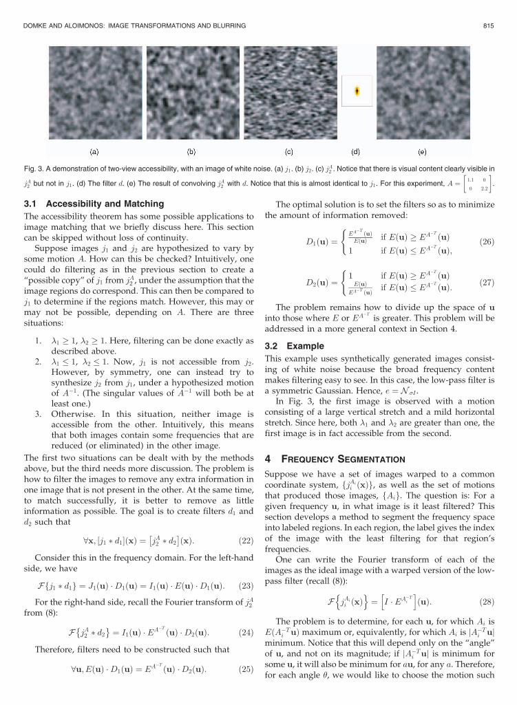
This example uses synthetically generated images consist-ing of white noise because the broad frequency contentmakes filtering easy to see. In this case, the low-pass filter isa symmetric Gaussian. Hence, e ¼ N �I .

In Fig. 3, the first image is observed with a motionconsisting of a large vertical stretch and a mild horizontalstretch. Since here, both �1 and �2 are greater than one, thefirst image is in fact accessible from the second.

4 FREQUENCY SEGMENTATION

Suppose we have a set of images warped to a commoncoordinate system, fjAi

i ðxÞg, as well as the set of motionsthat produced those images, fAig. The question is: For agiven frequency u, in what image is it least filtered? Thissection develops a method to segment the frequency spaceinto labeled regions. In each region, the label gives the indexof the image with the least filtering for that region’sfrequencies.

One can write the Fourier transform of each of theimages as the ideal image with a warped version of the low-pass filter (recall (8)):

F jAi

i ðxÞn o

¼ I � EA�Ti

h iðuÞ: ð28Þ

The problem is to determine, for each u, for which Ai isEðA�Ti uÞ maximum or, equivalently, for which Ai is jA�Ti ujminimum. Notice that this will depend only on the “angle”of u, and not on its magnitude; if jA�Ti uj is minimum forsome u, it will also be minimum for au, for any a. Therefore,for each angle �, we would like to choose the motion such


Fig. 3. A demonstration of two-view accessibility, with an image of white noise. (a) j1. (b) j2. (c) jA2 . Notice that there is visual content clearly visible in

jA2 but not in j1. (d) The filter d. (e) The result of convolving jA2 with d. Notice that this is almost identical to j1. For this experiment, A ¼ 1:1 0

0 2:2

� �.

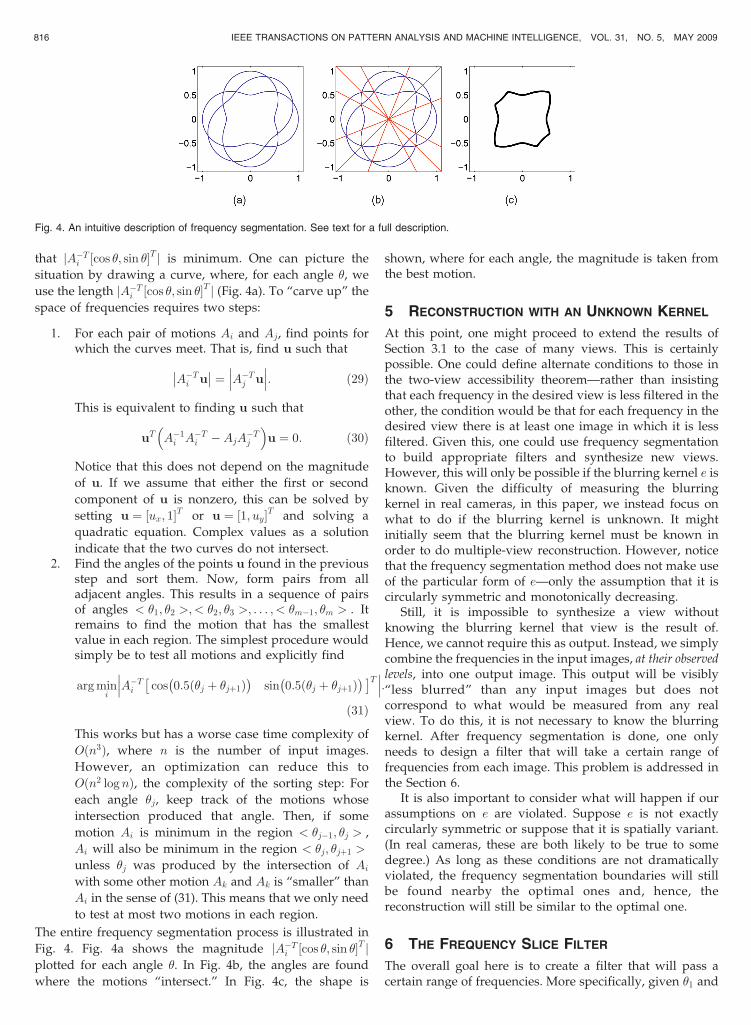
that jA�Ti ½cos �; sin ��T j is minimum. One can picture the

situation by drawing a curve, where, for each angle �, we

use the length jA�Ti ½cos �; sin ��T j (Fig. 4a). To “carve up” the

space of frequencies requires two steps:

1. For each pair of motions Ai and Aj, find points forwhich the curves meet. That is, find u such that

A�Ti u ¼ A�Tj u

: ð29Þ

This is equivalent to finding u such that

uT A�1i A�Ti �AjA

�Tj

� �u ¼ 0: ð30Þ

Notice that this does not depend on the magnitude

of u. If we assume that either the first or second

component of u is nonzero, this can be solved by

setting u ¼ ½ux; 1�T or u ¼ ½1; uy�T and solving a

quadratic equation. Complex values as a solution

indicate that the two curves do not intersect.2. Find the angles of the points u found in the previous

step and sort them. Now, form pairs from alladjacent angles. This results in a sequence of pairsof angles < �1; �2 >;< �2; �3 >; . . . ; < �m�1; �m > . Itremains to find the motion that has the smallestvalue in each region. The simplest procedure wouldsimply be to test all motions and explicitly find

arg miniA�Ti cos 0:5ð�j þ �jþ1Þ

� �sin 0:5ð�j þ �jþ1Þ� �� T :

ð31Þ

This works but has a worse case time complexity of

Oðn3Þ, where n is the number of input images.

However, an optimization can reduce this to

Oðn2 lognÞ, the complexity of the sorting step: For

each angle �j, keep track of the motions whose

intersection produced that angle. Then, if some

motion Ai is minimum in the region < �j�1; �j > ,

Ai will also be minimum in the region < �j; �jþ1 >

unless �j was produced by the intersection of Ai

with some other motion Ak and Ak is “smaller” than

Ai in the sense of (31). This means that we only need

to test at most two motions in each region.

The entire frequency segmentation process is illustrated in

Fig. 4. Fig. 4a shows the magnitude jA�Ti ½cos �; sin ��T jplotted for each angle �. In Fig. 4b, the angles are found

where the motions “intersect.” In Fig. 4c, the shape is

shown, where for each angle, the magnitude is taken fromthe best motion.

5 RECONSTRUCTION WITH AN UNKNOWN KERNEL

At this point, one might proceed to extend the results ofSection 3.1 to the case of many views. This is certainlypossible. One could define alternate conditions to those inthe two-view accessibility theorem—rather than insistingthat each frequency in the desired view is less filtered in theother, the condition would be that for each frequency in thedesired view there is at least one image in which it is lessfiltered. Given this, one could use frequency segmentationto build appropriate filters and synthesize new views.However, this will only be possible if the blurring kernel e isknown. Given the difficulty of measuring the blurringkernel in real cameras, in this paper, we instead focus onwhat to do if the blurring kernel is unknown. It mightinitially seem that the blurring kernel must be known inorder to do multiple-view reconstruction. However, noticethat the frequency segmentation method does not make useof the particular form of e—only the assumption that it iscircularly symmetric and monotonically decreasing.

Still, it is impossible to synthesize a view withoutknowing the blurring kernel that view is the result of.Hence, we cannot require this as output. Instead, we simplycombine the frequencies in the input images, at their observedlevels, into one output image. This output will be visibly“less blurred” than any input images but does notcorrespond to what would be measured from any realview. To do this, it is not necessary to know the blurringkernel. After frequency segmentation is done, one onlyneeds to design a filter that will take a certain range offrequencies from each image. This problem is addressed inthe Section 6.

It is also important to consider what will happen if ourassumptions on e are violated. Suppose e is not exactlycircularly symmetric or suppose that it is spatially variant.(In real cameras, these are both likely to be true to somedegree.) As long as these conditions are not dramaticallyviolated, the frequency segmentation boundaries will stillbe found nearby the optimal ones and, hence, thereconstruction will still be similar to the optimal one.

6 THE FREQUENCY SLICE FILTER

The overall goal here is to create a filter that will pass acertain range of frequencies. More specifically, given �1 and


Fig. 4. An intuitive description of frequency segmentation. See text for a full description.

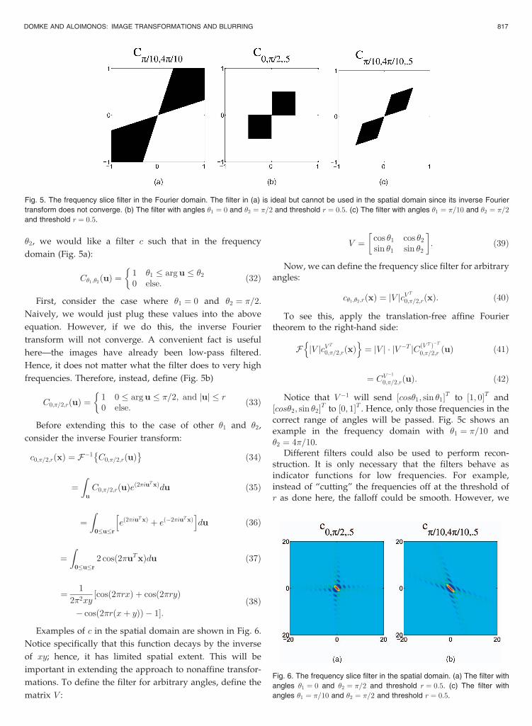
�2, we would like a filter c such that in the frequency

domain (Fig. 5a):

C�1;�2ðuÞ ¼ 1 �1 � arg u � �2

0 else:

ð32Þ

First, consider the case where �1 ¼ 0 and �2 ¼ �=2.

Naively, we would just plug these values into the above

equation. However, if we do this, the inverse Fourier

transform will not converge. A convenient fact is useful

here—the images have already been low-pass filtered.

Hence, it does not matter what the filter does to very high

frequencies. Therefore, instead, define (Fig. 5b)

C0;�=2;rðuÞ ¼1 0 � arg u � �=2; and juj � r0 else:

ð33Þ

Before extending this to the case of other �1 and �2,

consider the inverse Fourier transform:

c0;�=2;rðxÞ ¼ F�1 C0;�=2;rðuÞ�

ð34Þ

¼Z

u

C0;�=2;rðuÞeð2�iuTxÞdu ð35Þ

¼Z

0�u�r

eð2�iuTxÞ þ eð�2�iuTxÞ

h idu ð36Þ

¼Z

0�u�r

2 cosð2�uTxÞdu ð37Þ

¼ 1

2�2xycosð2�rxÞ þ cosð2�ryÞ½

� cos 2�rðxþ yÞð Þ � 1�:ð38Þ

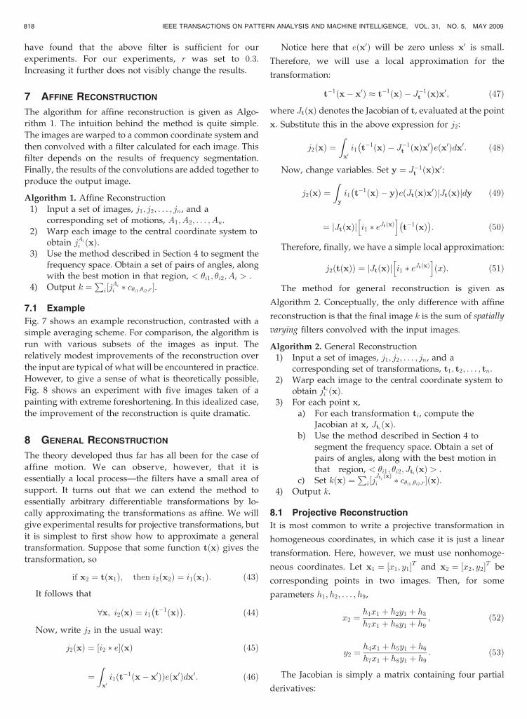
Examples of c in the spatial domain are shown in Fig. 6.

Notice specifically that this function decays by the inverse

of xy; hence, it has limited spatial extent. This will be

important in extending the approach to nonaffine transfor-

mations. To define the filter for arbitrary angles, define the

matrix V :

V ¼ cos �1 cos �2

sin �1 sin �2

� �: ð39Þ

Now, we can define the frequency slice filter for arbitraryangles:

c�1;�2;rðxÞ ¼ jV jcVT

0;�=2;rðxÞ: ð40Þ

To see this, apply the translation-free affine Fouriertheorem to the right-hand side:

F jV jcV T

0;�=2;rðxÞn o

¼ jV j � jV �T jCðVT Þ�T

0;�=2;r ðuÞ ð41Þ

¼ CV �1

0;�=2;rðuÞ: ð42Þ

Notice that V �1 will send ½cos�1; sin �1�T to ½1; 0�T and½cos�2; sin �2�T to ½0; 1�T . Hence, only those frequencies in thecorrect range of angles will be passed. Fig. 5c shows anexample in the frequency domain with �1 ¼ �=10 and�2 ¼ 4�=10.

Different filters could also be used to perform recon-struction. It is only necessary that the filters behave asindicator functions for low frequencies. For example,instead of “cutting” the frequencies off at the threshold ofr as done here, the falloff could be smooth. However, we


Fig. 5. The frequency slice filter in the Fourier domain. The filter in (a) is ideal but cannot be used in the spatial domain since its inverse Fourier

transform does not converge. (b) The filter with angles �1 ¼ 0 and �2 ¼ �=2 and threshold r ¼ 0:5. (c) The filter with angles �1 ¼ �=10 and �2 ¼ �=2and threshold r ¼ 0:5.

Fig. 6. The frequency slice filter in the spatial domain. (a) The filter with

angles �1 ¼ 0 and �2 ¼ �=2 and threshold r ¼ 0:5. (c) The filter with

angles �1 ¼ �=10 and �2 ¼ �=2 and threshold r ¼ 0:5.

have found that the above filter is sufficient for our

experiments. For our experiments, r was set to 0:3.

Increasing it further does not visibly change the results.

7 AFFINE RECONSTRUCTION

The algorithm for affine reconstruction is given as Algo-

rithm 1. The intuition behind the method is quite simple.

The images are warped to a common coordinate system and

then convolved with a filter calculated for each image. This

filter depends on the results of frequency segmentation.

Finally, the results of the convolutions are added together to

produce the output image.

Algorithm 1. Affine Reconstruction

1) Input a set of images, j1; j2; . . . ; jn, and a

corresponding set of motions, A1; A2; . . . ; An.

2) Warp each image to the central coordinate system to

obtain jAi

i ðxÞ.3) Use the method described in Section 4 to segment the

frequency space. Obtain a set of pairs of angles, along

with the best motion in that region, < �i1; �i2; Ai > .

4) Output k ¼P

i½jAi

i � c�i1;�i2;r�.

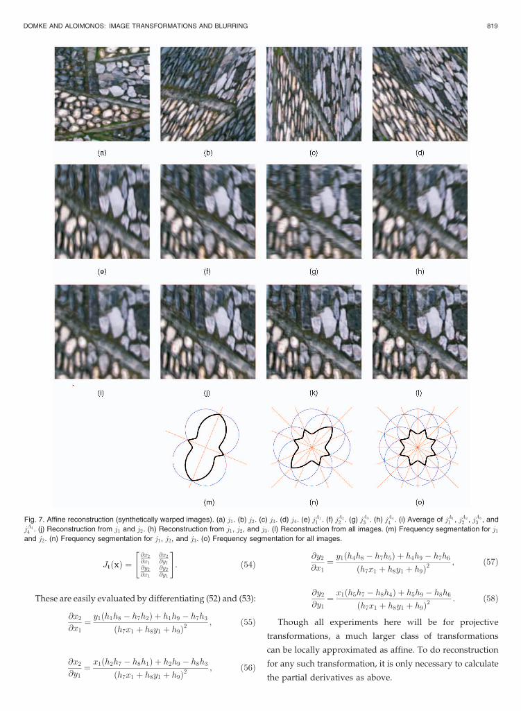
7.1 Example

Fig. 7 shows an example reconstruction, contrasted with a

simple averaging scheme. For comparison, the algorithm is

run with various subsets of the images as input. The

relatively modest improvements of the reconstruction over

the input are typical of what will be encountered in practice.

However, to give a sense of what is theoretically possible,

Fig. 8 shows an experiment with five images taken of a

painting with extreme foreshortening. In this idealized case,

the improvement of the reconstruction is quite dramatic.

8 GENERAL RECONSTRUCTION

The theory developed thus far has all been for the case of

affine motion. We can observe, however, that it is

essentially a local process—the filters have a small area of

support. It turns out that we can extend the method to

essentially arbitrary differentiable transformations by lo-

cally approximating the transformations as affine. We will

give experimental results for projective transformations, but

it is simplest to first show how to approximate a general

transformation. Suppose that some function tðxÞ gives the

transformation, so

if x2 ¼ tðx1Þ; then i2ðx2Þ ¼ i1ðx1Þ: ð43Þ

It follows that

8x; i2ðxÞ ¼ i1 t�1ðxÞ� �

: ð44Þ

Now, write j2 in the usual way:

j2ðxÞ ¼ ½i2 � e�ðxÞ ð45Þ

¼Z

x0i1ðt�1 x� x0Þð Þeðx0Þdx0: ð46Þ

Notice here that eðx0Þ will be zero unless x0 is small.

Therefore, we will use a local approximation for the

transformation:

t�1ðx� x0Þ t�1ðxÞ � J�1t ðxÞx0; ð47Þ

where JtðxÞ denotes the Jacobian of t, evaluated at the point

x. Substitute this in the above expression for j2:

j2ðxÞ ¼Z

x0i1 t�1ðxÞ � J�1

t ðxÞx0� �

eðx0Þdx0: ð48Þ

Now, change variables. Set y ¼ J�1t ðxÞx0:

j2ðxÞ ¼Z

y

i1 t�1ðxÞ � y� �

e JtðxÞx0ð Þ JtðxÞj jdy ð49Þ

¼ JtðxÞj j i1 � eJtðxÞh i

t�1ðxÞ� �

: ð50Þ

Therefore, finally, we have a simple local approximation:

j2 tðxÞð Þ ¼ JtðxÞj j i1 � eJtðxÞh i

ðxÞ: ð51Þ

The method for general reconstruction is given as

Algorithm 2. Conceptually, the only difference with affine

reconstruction is that the final image k is the sum of spatially

varying filters convolved with the input images.

Algorithm 2. General Reconstruction

1) Input a set of images, j1; j2; . . . ; jn, and a

corresponding set of transformations, t1; t2; . . . ; tn.

2) Warp each image to the central coordinate system to

obtain jtii ðxÞ.3) For each point x,

a) For each transformation ti, compute the

Jacobian at x, JtiðxÞ.b) Use the method described in Section 4 to

segment the frequency space. Obtain a set of

pairs of angles, along with the best motion in

that region, < �i1; �i2; JtiðxÞ > .

c) Set kðxÞ ¼P

i½jJtiðxÞ

i � c�i1;�i2;r�ðxÞ.4) Output k.

8.1 Projective Reconstruction

It is most common to write a projective transformation in

homogeneous coordinates, in which case it is just a linear

transformation. Here, however, we must use nonhomoge-

neous coordinates. Let x1 ¼ ½x1; y1�T and x2 ¼ ½x2; y2�T be

corresponding points in two images. Then, for some

parameters h1; h2; . . . ; h9,

x2 ¼h1x1 þ h2y1 þ h3

h7x1 þ h8y1 þ h9; ð52Þ

y2 ¼h4x1 þ h5y1 þ h6

h7x1 þ h8y1 þ h9: ð53Þ

The Jacobian is simply a matrix containing four partial

derivatives:


JtðxÞ ¼@x2

@x1

@x2

@y1@y2

@x1

@y2

@y1

" #: ð54Þ

These are easily evaluated by differentiating (52) and (53):

@x2

@x1¼ y1ðh1h8 � h7h2Þ þ h1h9 � h7h3

ðh7x1 þ h8y1 þ h9Þ2; ð55Þ

@x2

@y1¼ x1ðh2h7 � h8h1Þ þ h2h9 � h8h3


@y2

@x1¼ y1ðh4h8 � h7h5Þ þ h4h9 � h7h6


@y2

@y1¼ x1ðh5h7 � h8h4Þ þ h5h9 � h8h6

ðh7x1 þ h8y1 þ h9Þ2: ð58Þ

Though all experiments here will be for projective

transformations, a much larger class of transformations

can be locally approximated as affine. To do reconstruction

for any such transformation, it is only necessary to calculate

the partial derivatives as above.


Fig. 7. Affine reconstruction (synthetically warped images). (a) j1. (b) j2. (c) j3. (d) j4. (e) jA11 . (f) jA2

2 . (g) jA3

3 . (h) jA4

4 . (i) Average of jA11 , jA2

2 , jA3

3 , and

jA4

4 . (j) Reconstruction from j1 and j2. (h) Reconstruction from j1, j2, and j3. (l) Reconstruction from all images. (m) Frequency segmentation for j1

and j2. (n) Frequency segmentation for j1, j2, and j3. (o) Frequency segmentation for all images.

8.2 Making Reconstruction Faster

For affine reconstruction, the algorithm is extremely

fast—the computation is dominated by the convolutions

in step 4. In the algorithm for general reconstruction,

however, the filters are spatially varying and need to be

recalculated at each pixel.A simple trick can speed this up. Instead of calculating

the filters for each pixel, calculate them for some small

patch of pixels. If the affine approximation is slowly

changing, this will result in no visible change to the output,

while hugely reducing the overhead for recomputing filters.

However, this strategy could introduce artifacts on some

images, at the boundary where the filters change. To reduce

this, we allow the patches to overlap by one pixel and use a

small amount of blending. For pixels in overlapping

regions, the output is set to the average of the results of

the different filters. In our experiments, we used patches of

size 20 � 20.

8.3 Experiments

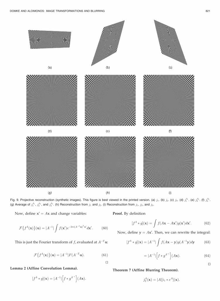
Fig. 9 shows a reconstruction from three synthetically

generated images of a radius pattern. We compare our

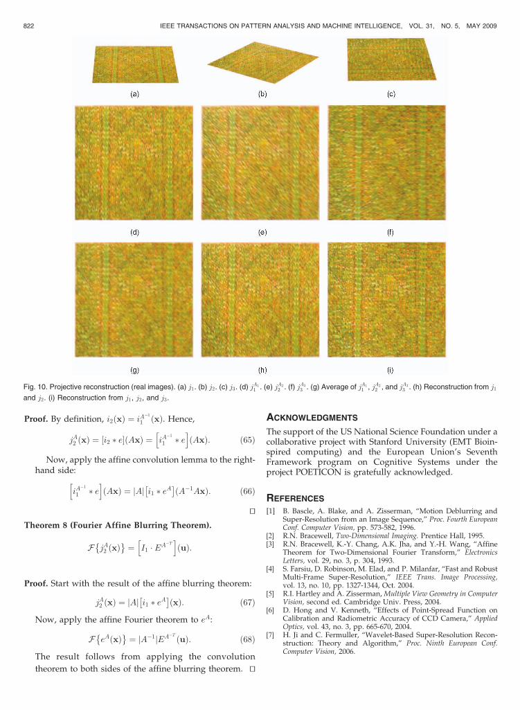
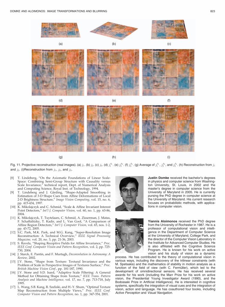
results to a simple averaging process.Figs. 10 and 11 show the reconstruction process for

images taken of two different textures. After reconstruction,

for presentation, we manually segmented out the back-

ground. To better understand how using more images leads

to better reconstruction, we also include the results of

reconstruction using only the first two of the three images.

9 CONCLUSIONS

This paper introduced the formalism of the “ideal image,”

consisting of the unblurred incoming light, and the “real

image,” consisting of the blurred measured image. Because

this framework separates the filtering and geometrical

aspects, it makes it easy to derive several results. The notion

of the ideal image might be useful for deriving other results.

More formally, a relation between the outputs of filters

applied at corresponding patches in different views was

developed. This result was used to formulate and prove the

accessibility theorem, which states the conditions under

which, given two images of the same scene, one is accessible

by the other (i.e., one image can be obtained by appro-

priately filtering the other). We then discussed the con-

sequences of this result to the understanding of the space of

all images of a scene. As an application of this framework,

we showed that it is possible to perform multiple-view

image reconstruction, even with an unknown blurring

kernel, through the new tool of frequency segmentation.

APPENDIX

Theorem 6 (Translation-Free Affine Fourier Theorem). IfFffðxÞg ¼ F ðuÞ, then FffAðxÞg ¼ jA�1jFA�T ðuÞ.

Proof.

F fAðxÞ�

ðuÞ ¼ZfðAxÞe�2�iuTxdx: ð59Þ


Fig. 8. Affine reconstruction with extreme foreshortening. (synthetically warped images). (a) j1. (b) j2. (c) j3. (d) j4. (e) j5. (f) jA1

1 . (g) jA2

2 . (h) jA3

3 . (i) jA4

4 .

(j) jA5

5 . (k) Average of jA1

1 . . . jA5

4 . (l) Reconstruction from j1 and j2. (m) Reconstruction from j1, j2, and j3. (n) Reconstruction from j1 . . . j4.

(o) Reconstruction from all images.

Now, define x0 ¼ Ax and change variables:

F fAðxÞ�

ðuÞ ¼ jA�1jZfðx0Þe�2�iðA�TuÞTx0dx0: ð60Þ

This is just the Fourier transform of f , evaluated at A�Tu:

F fAðxÞ�

ðuÞ ¼ jA�1jF ðA�TuÞ: ð61Þ

tuLemma 2 (Affine Convolution Lemma).

½fA � g�ðxÞ ¼ jA�1j f � gA�1h i

ðAxÞ:

Proof. By definition

½fA � g�ðxÞ ¼ZfðAx�Ax0Þgðx0Þdx0: ð62Þ

Now, define y ¼ Ax0. Then, we can rewrite the integral:

½fA � g�ðxÞ ¼ jA�1jZfðAx� yÞgðA�1yÞdy ð63Þ

¼ jA�1j f � gA�1h i

ðAxÞ: ð64Þ

tuTheorem 7 (Affine Blurring Theorem).

jA2 ðxÞ ¼ jAj½i1 � eA�ðxÞ:


Fig. 9. Projective reconstruction (synthetic images). This figure is best viewed in the printed version. (a) j1. (b) j2. (c) j3. (d) jA1

1 . (e) jA2

2 . (f) jA3

3 .

(g) Average of jA1

1 , jA2

2 , and jA3

3 . (h) Reconstruction from j1 and j2. (i) Reconstruction from j1, j2, and j3.

Proof. By definition, i2ðxÞ ¼ iA�1

1 ðxÞ. Hence,

jA2 ðxÞ ¼ ½i2 � e�ðAxÞ ¼ iA�1

1 � eh i

ðAxÞ: ð65Þ

Now, apply the affine convolution lemma to the right-hand side:

iA�1

1 � eh i

ðAxÞ ¼ jAj i1 � eA� �

ðA�1AxÞ: ð66Þ

tuTheorem 8 (Fourier Affine Blurring Theorem).

F jA2 ðxÞ�

¼ I1 � EA�Th i

ðuÞ:

Proof. Start with the result of the affine blurring theorem:

jA2 ðxÞ ¼ jAj i1 � eA� �

ðxÞ: ð67Þ

Now, apply the affine Fourier theorem to eA:

F eAðxÞ�

¼ jA�1jEA�T ðuÞ: ð68Þ

The result follows from applying the convolution

theorem to both sides of the affine blurring theorem. tu

ACKNOWLEDGMENTS

The support of the US National Science Foundation under acollaborative project with Stanford University (EMT Bioin-spired computing) and the European Union’s SeventhFramework program on Cognitive Systems under theproject POETICON is gratefully acknowledged.

REFERENCES

[1] B. Bascle, A. Blake, and A. Zisserman, “Motion Deblurring andSuper-Resolution from an Image Sequence,” Proc. Fourth EuropeanConf. Computer Vision, pp. 573-582, 1996.

[2] R.N. Bracewell, Two-Dimensional Imaging. Prentice Hall, 1995.[3] R.N. Bracewell, K.-Y. Chang, A.K. Jha, and Y.-H. Wang, “Affine

Theorem for Two-Dimensional Fourier Transform,” ElectronicsLetters, vol. 29, no. 3, p. 304, 1993.

[4] S. Farsiu, D. Robinson, M. Elad, and P. Milanfar, “Fast and RobustMulti-Frame Super-Resolution,” IEEE Trans. Image Processing,vol. 13, no. 10, pp. 1327-1344, Oct. 2004.

[5] R.I. Hartley and A. Zisserman, Multiple View Geometry in ComputerVision, second ed. Cambridge Univ. Press, 2004.

[6] D. Hong and V. Kenneth, “Effects of Point-Spread Function onCalibration and Radiometric Accuracy of CCD Camera,” AppliedOptics, vol. 43, no. 3, pp. 665-670, 2004.

[7] H. Ji and C. Fermuller, “Wavelet-Based Super-Resolution Recon-struction: Theory and Algorithm,” Proc. Ninth European Conf.Computer Vision, 2006.


Fig. 10. Projective reconstruction (real images). (a) j1. (b) j2. (c) j3. (d) jA1

1 . (e) jA2

2 . (f) jA3

3 . (g) Average of jA1

1 , jA2

2 , and jA3

3 . (h) Reconstruction from j1

and j2. (i) Reconstruction from j1, j2, and j3.

[8] T. Lindeberg, “On the Axiomatic Foundations of Linear Scale-Space: Combining Semi-Group Structure with Causality versusScale Invariance,” technical report, Dept. of Numerical Analysisand Computing Science, Royal Inst. of Technology, 1994.

[9] T. Lindeberg and J. Garding, “Shape-Adapted Smoothing inEstimation of 3-D Shape Cues from Affine Deformations of Local2-D Brightness Structure,” Image Vision Computing, vol. 15, no. 6,pp. 415-434, 1997.

[10] K. Mikolajczyk and C. Schmid, “Scale & Affine Invariant InterestPoint Detectors,” Int’l J. Computer Vision, vol. 60, no. 1, pp. 63-86,2004.

[11] K. Mikolajczyk, T. Tuytelaars, C. Schmid, A. Zisserman, J. Matas,F. Schaffalitzky, T. Kadir, and L. Van Gool, “A Comparison ofAffine Region Detectors,” Int’l J. Computer Vision, vol. 65, nos. 1-2,pp. 43-72, 2005.

[12] S.C. Park, M.K. Park, and M.G. Kang, “Super-Resolution ImageReconstruction: A Technical Overview,” IEEE Signal ProcessingMagazine, vol. 20, no. 3, pp. 21-36, 2003.

[13] S. Ravela, “Shaping Receptive Fields for Affine Invariance,” Proc.IEEE Conf. Computer Vision and Pattern Recognition, vol. 2, pp. 725-730, 2004.

[14] J. Starck, E. Pantin, and F. Murtagh, Deconvolution in Astronomy: AReview, 2002.

[15] J.V. Stone, “Shape from Texture: Textural Invariance and theProblem of Scale in Perspective Images of Textures Surface,” Proc.British Machine Vision Conf., pp. 181-187, 1990.

[16] J.V. Stone and S.D. Isard, “Adaptive Scale Filtering: A GeneralMethod for Obtaining Shape from Texture,” IEEE Trans. PatternAnalysis and Machine Intelligence, vol. 17, no. 7, pp. 713-718, July1995.

[17] L. Wang, S.B. Kang, R. Szeliski, and H.-Y. Shum, “Optimal TextureMap Reconstruction from Multiple Views,” Proc. IEEE Conf.Computer Vision and Pattern Recognition, no. 1, pp. 347-354, 2001.

Justin Domke received the bachelor’s degreesin physics and computer science from Washing-ton University, St. Louis, in 2002 and themaster’s degree in computer science from theUniversity of Maryland in 2005. He is currentlypursing the PhD degree in computer science atthe University of Maryland. His current researchfocuses on probabilistic methods, with applica-tions in computer vision.

Yiannis Aloimonos received the PhD degreefrom the University of Rochester in 1987. He is aprofessor of computational vision and intelli-gence in the Department of Computer Scienceat the University of Maryland, College Park, andthe director of the Computer Vision Laboratory inthe Institute for Advanced Computer Studies. Heis also affiliated with the Cognitive ScienceProgram. He is known for his work on activevision and his study of vision as a dynamic

process. He has contributed to the theory of computational vision invarious ways, including the discovery of the trilinear constraints (withM. Spetsakis) and the mathematics of stability in motion analysis as afunction of the field of view (with C. Fermuller), which led to thedevelopment of omnidirectional sensors. He has received severalawards for his work (including the Marr Prize for his work on activevision, the Presidential Young Investigator Award (1990), and theBodossaki Prize in Artificial Intelligence). He is interested in cognitivesystems, specifically the integration of visual cues and the integration ofvision, action and language. He has coauthored four books, includingActive Perception and Visual Navigation.


Fig. 11. Projective reconstruction (real images). (a) j1. (b) j2. (c) j3. (d) jA1

1 . (e) jA2

2 . (f) jA3

3 . (g) Average of jA1

1 , jA2

2 , and jA3

3 . (h) Reconstruction from j1

and j2. (i)Reconstruction from j1, j2, and j3.

Documents

Image Transformations and Blurring