Embed Size (px)
Citation preview
Image Wavelet Decompositionand Applications
N. Treil, S. Mallat
R. Bajcsy
MS-CIS-89-22
GRASP LAB 177
-
.!f_)j-i '_._L;
Department of Computer and Information Science
School of Engineering and Applied ScienceUniversity of Pennsylvania
Philadelphia, PA 19104
April 1989
Acknowledgements: This research was supported in part by Air Force AFOSRF49620-85-K-0018, U.S. Army grants DAA29-84-K-0061, DAA29-84-9-0027, NOO14-85-K-0807, NSF grants MCS-8219196-CER, IRI84-10413-AO2, INT85-14199, DMC85-17315, NIHNS-10939-11 as part of the Cerebro Vascular Research Center, NIH 1-RO1-NS-23636-01,NATO grant 0224/85, NASA NAG5-1045, ONR SB-35923-0, DARPA grant NOOO14-85-K-0018, and by DEC Corporation, IBM Corporation and LORD Corporation.
(AIASA.-C_-188.217) IMAGE WAVELET
DECOMPOSITION AND APPLICATIONS
(P_nnsylvani_ Univ.) 43 CSCL 09_
G3/o3
N9 L-Z 3787
https://ntrs.nasa.gov/search.jsp?R=19910014474 2020-03-04T14:28:22+00:00Z

A CKN O WLED G EMENT S.
Nicolas Treil
I am particularly grateful to Ruzena Bajcsy who guided me through this whole project
and who contributed to most of the ideas and concepts of the edge detection applications.
I am also very grateful to Stephane Mallat for the time he spent introducing me to the
theory of wavelets, and for supervising all the signal processing part of this work. I received
a lot of help from Jing Zhao and Howie Choset on this particular project. I would also
like to thank for their patience and helpful hints : Scott Alexander, Helen Anderson, Trevor
Darell, Doug Earhart, Alberto Izaguirre, Douglas Katzman, Sang Lee, Raymond McKendall,
Suzanne Morin, Arup Mukherjee, Yves Schabes and Steve Sherin. I enjoyed many valuable
discussions with Ales Leonardis. Finally I would like to thank my parents for their moral
and financial support.
Edited by Howie Choset.
I am grateful to Dr. R. Bajcsy for letting me work on this project. I would like to thank
Helen Anderson for her constant support and understanding throughout my time on this
project. Raymond KcKendall's assistance was both useful and educational. I am grateful
to him for the time and effort he put into me and this project. Thank you Arup Mukherjee
for the helping me modify Nicolas' system. I would like to thank Scott Alexander for his
assistance at ten to five on Friday afternoons. I would also like to thank Dr. Richard Paul
and Dr. Anthony D'Amico for their constant moral support. Finally, I would like to thank
James Lotkowski for his patience.
Abstract
The general problem of computer vision has been investigated for more than twenty years
and is still one of the most challenging fields in artificial intelligence. Indeed taking a look
at the human visual system can give us an idea of the complexity of any solution to the
problem of visual recognition. This general task can be decomposed into a whole hierarchy
of problems ranging from pixel processing to high level segmentation and complex objects
recognition.
Contrasting an image at different representations provides useful information such as
edges. First, we introduce an example of low level signal and image processing using the
theory of wavelets which provides the basis for multiresolution representation. Like the
human brain, we use a multiorientation process which detects features independently in
different orientation sectors. So, we end up contrasting images of the same orientation but
of different resolutions to gather information about an image.
We then develop an interesting image representation using energy zero crossings. We
show that this representation is experimentally complete and leads to some higher level
applications such as edge and corner finding, which in turn provides two basic steps to
image segmentation. We also discuss the possibilities of feedback between different levels of
processing.

Contents
1 Introduction. 3
2 The multiresolution concept.
2.1 Motivation .....................................
2.2 The theory of wavelets ...............................
3 The multiorientation concept.
4 The decomposition process.
3
5
3
4
4
5
4.1 Monodimensional dyadic wavelet decomposition ................. 5
4.2 Bidimensional dyadic wavelet decomposition ................... 10
4.3 Energy-zero-crossings representation ....................... 13
Completeness of the representations. 17
5.1 Dyadic wavelet transform ............................. 17
5.1.1 One dimensionnal algorithm ........................ 17
5.2
Two dimensionnal algorithm ....................... 18
Completeness of the Energy-zero-crossings representation ............ 20
5.1.2
6 Applications to higher level vision processes.
Edge detection ...................................
6.1.1 Basic edge-detection algorithm ......................
6.1
23
23
23

A
6.1.2
6.1.3
Algorithm improvement ..........................
Edge finding and multiorientation ....................
6.2 Corner detection..................................
6.2.1
6.2.2
Algorithm ..................................
Corner resolution ..............................
24
29
29
3O
32
6.3 Unconnected lines detection: an example of feed-back.............. 34
Dyadic decomposition with an expansion by 2. 34
A.1 One dimensional algorithm ............................ 34
A.2 Two dimensional algorithm ............................ 36
B Coefficients of wavelet filters. 37
C Clustering algorithm. 37
2
1 Introduction.
The general problem of computer vision has been investigated for more than twenty years
and is still one of the most challenging fields in artificial intelligence. Just by taking a look
at the human visual system can give us an idea of the complexity of any solution to the
problem of visual recognition. This general task can be decomposed into a whole hierarchy
of problems ranging from pixel processing to high level segmentation and complex objects
recognition. First, we introduce an example of low level signal and image processing using
the theory of wavelets and then develop interesting image representation. We show that this
representation is experimentally complete and leads to some higher level applications such
as edge and corner finding. This, in turn, provides two basic steps to image segmentation.
We also discuss the possibilities of feedback between different levels of processing.
2 The multiresolution concept.
2.1 Motivation.
The information provided by an image lies in the local variations of the image intensity.
From the image contrast, we can extract some important features such as the edges of the
structures embedded in the image. At the border of such structures, the image intensity is
likely to suddenly change. The local variations have therefore a high amplitude.
However not all of the local variations have the same relevance to the understanding of
a scene. For example, suppose that we are looking at a far away house. Moving closer to it
would make us distinguish successively the doors and windows, then the bricks of the walls
and the tiles, then the texture of these bricks and tiles. Separating the details appearing at
each resolution would enable us to establish a hierarchy between these pieces of information.
It would also allow a scale-invariant interpretation of the image. This scale invariance is a
well known property of the human visual system.
As it is not possible to define a priori an optimal resolution for analyzing images, several
researchers have developed pattern matching algorithms which process the image at different
resolutions. In some sense, image's details at a coarse resolution provide the "context" of
the image which helps in the analysis of finer details. For example, it is difficult to recognize
that a small rectangle inside an image is the window of a house if we did not previously
recognize the house "context". It is therefore natural to first analyze the image details at a
coarse resolution and then increase the resolution using a coarse to fine processing strategy.
Another interesting approach is to study details' propagation through different resolutions.
A feature which appears at several resolutions is certainly very noticeable in the image and
is likely to be part of an object's contour. A feature appearing only at finer resolutions is a
3
high frequency variation of small amplitude. It probably corresponds to some texture. On
the other hand, a feature which appears only at coarse resolutions is a smooth variation like
shading.
2.2 The theory of wavelets.
Recently Stephane Mallat has introduced such a multiresolution representation of signals
based on the theory of wavelets [1], using a finite set of resolutions namely the powers of 2 (a
definite advantage for implementation). The basic idea is to separate the higher half and the
lower half of the spectrum of a signal by using a second order band-pass filter and a low pass
filter, to subsample the image corresponding to the lower half of the spectrum and to iterate
the process. This is roughly equivalent to dividing the spectrum in successive bands [_,_r],
[_, _], Is, _] "'" [2-_+_, _] and extracting independently the details corresponding to these
bands. Suppose that our original signal has 2 j samples. It is then said to be at resolution 2 j.
The result of the first band-pass filtering will give us the difference of information between
resolution 2 j and resolution 2 j-1. The result of the next band-pass filtering will give us the
difference of information between resolution 2 j-1 and resolution 2 j-2 and so on. The theory
of wavelets shows that we can obtain filters which are very well localized both in the Fourier
and spatial domain --thus preserving the locality of information-- and that we can achieve
a representation which is complete.
In order to obtain a representation of the signal which translates when the signal translate,
Stephane Mallat[2] has designed another type of representation of the band-pass filtered
images based on their zero-crossings and the energies between consecutive zero-crossings.
It is called an Energy-zero-crossings representation. This representation has proved to be
experimentally complete for signals [1] and in this article we also show that it is complete
for images. It is the basis of the higher level applications developed in this article.
3 The multiorientation concept.
The purpose of a multiorientation process is to detect features independently in different
orientation sectors. Although this increases the amount of computation, it also structures the
data organization of the feature detection processes. Let us take a simple example. Suppose
we carry out isotropic edge detection on an image which contains a rectangle. It would be
pretty difficult to recognize that the closed region we have detected is actually a rectangle;
one obstacle among others is that most edge detectors smooth corners[3]. If on the other
hand we detect horizontal edges and vertical edges independently, and then use a composition
process to find closed regions from the interactions between these edges, we will define an
object with two horizontal sides two vertical sides and four corners ... obviously a rectangle !
In both case the result of the analysis is a closed region but by using multiorientation we
4

have learned something about the shape of the region while building it. Of course this is avery simplistic example and the composition processesare far from being straightforward,but this gives a hint on the idea of any image analysis method based on decomposition:gaining knowledge while recomposing. We can of course think of gaining knowledge aboutthe organization of a sceneby using a composition process on multiresolution as well.
It is interesting to note that multiorientation is one of the features of the human vi-sion system[4]. Indeed there exist brain cells which respond specifically to stimuli within acertain orientation and also at a certain frequency. This means that the brain performs amultiresolution multiorientation decomposition of the visual input. There are asmany as 30main directions, where the divisions are finer around the horizontal and vertical axes. Therealso exist cells which respond specifically to corners. We can guessfrom this that the brainperforms some composition processing as part of the whole visual recognition system.
4 The decomposition process.
In this section we describe in detail the decomposition process leading to the Energy-zero-
crossings representation. Our purpose is not to explain the theory of wavelets. The choice
of the filters as well as certain properties like the completeness of the representation have
very sound mathematical bases which will not be discused here.
4.1 Monodimensional dyadic wavelet decomposition.
Let S j be a signal at resolution 2 j and W k be the signal of the differences between S k and
S k-1 for k less than or equal to j. Let U,_ be the low-pass filter with a cutoff frequency2
of _ and G-_ be the high-pass filter with a cutoff frequency of _. From the general idea of2
multiresolution, a simple processing would be:
1. Filter S j by G_ . The result is W j
2. Filter S j by U_ and sample by 2. The result is S j-1
3. Filter S j-1 by G_ . The result is W j-1
4. Filter S j-1 by U_ and sample by 2. The result is S j-2 and so on...
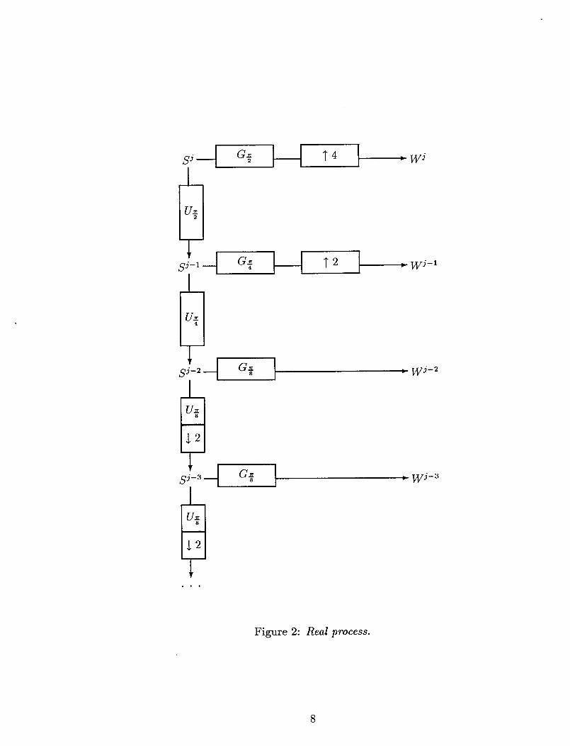
This process is summarized in Figure 1.
5

G_r2 * W j
G_- [ . Wj-1
Figure 1: Conceptual process.
The final goal of the decomposition is to obtain zero-crossings which point out some
information to us. In other word we would like them to correspond to abrupt changes
in the signal intensity. The energy associated with these zero-crossings would provide a
measurement of the abruptness of the variation. The other constraint is that we want
to build a multiresolution representation which is complete. This leads to two important
features of the decomposition process:
• To achieve the completeness of the Energy-zero-crossings representation, we need a
good precision on the zero-crossings. Thus we need to expand the results of the
consecutive band-pass filterings before computing the positions of the zeros. This is
done by performing a spline interpolation.
• The filters have to fit the requirements of the theory of wavelets. After computation
they appear to perform a rather smooth cutoff. Thus we cannot sample by two the re-
sult of the low-pass filtering without loosing information[5]. A solution to this problem
is to wait for several iterations of the process 1 before starting the actual sampling.
(W)ie[j-n..j] by aFrom what we have just said, supposing that we want to expand the i
factor 4 (typical expansion factor) the algorithm becomes:
1. Filter S j by G_ . The result is W j
1We call iteration the list of operations yielding the isolation of the spectrum part between _ and
6

2. Expand W i by a factor 4
3. Filter S j by U_ . The result is S j-1 (but it still has 2 j samples I)
4. Filter S j-1 by G_ . The result is W j-1
5. Expand W j-1 by a factor 2
6. Filter S j-1 by U_ . The result is S j-2
7. Filter S j-2 by G{ . The result is W j-2
8. Filter S j-2 by U_ and sample by 2. The result is S j-3
9. Filter S j-3 by G_ . The result is W j-3
10. Filter S j-3 by U_ and sample by 2. The result is S j-4 and so on...
This is summarized in Figure 2. In Appendix A we give the algorithm for an expansion
factor of 2 instead of 4.
SJ--
S _-_
SJ -_ -_
SJ -a -_
GTr2
a_4
a _8
8
T4 _- w j
. W J-2
WJ-S
Figure 2: Real process.
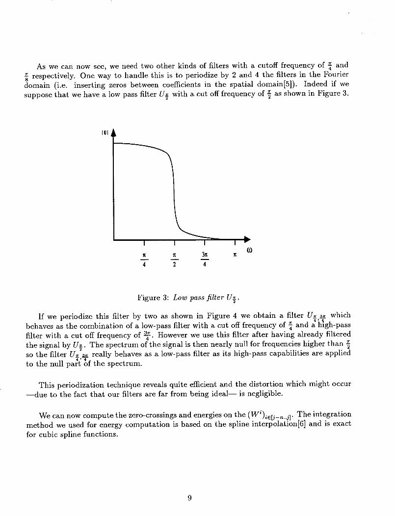
As we can now see, we need two other kinds of filters with a cutoff frequency of 4 and
8 respectively. One way to handle this is to periodize by 2 and 4 the filters in the Fourier
domain (i.e. inserting zeros between coefficients in the spatial domain[5]). Indeed if we
suppose that we have a low pass filter Ux with a cut off frequency of _ as shown in Figure 3.2
Iol
I ] ] [ v(O
_c 3_
4 2 4
Figure 3: Low pass filter U_-.2
If we periodize this filter by two as shown in Figure 4 we obtain a filter U__ 32 which
behaves as the combination of a low-pass filter with a cut off frequency of 4 and a high-pass
filter with a cut off frequency of -_. However we use this filter after having already filtered
the signal by U_. The spectrum of the signal is then nearly null for frequencies higher thanso the filter U__ 3_ really behaves as a low-pass filter as its high-pass capabilities are applied
4'
to the null part If the spectrum.
This periodization technique reveals quite efficient and the distortion which might occur
--due to the fact that our filters are far from being ideal-- is negligible.
We can now compute the zero-crossings and energies on the i(W)ie[j-n..j]" The integration
method we used for energy computation is based on the spline interpolation[6] and is exact
for cubic spline functions.
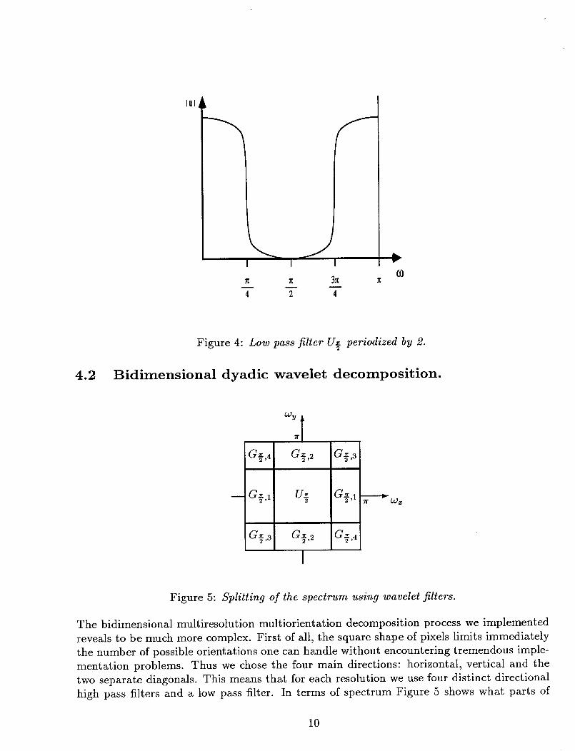
IuI
JI I I
n 3n
4 2 4
/tO)
4.2
Figure 4: Low pass filter U_ periodized by 2.
Bidimensional dyadic wavelet decomposition.
G_,4 G_,2 iG_,3
G_,I -"-'_w"ff x
G_,4
Figure 5: Splitting of the spectrum using wavelet filters.
The bidimensional multiresolution multiorientation decomposition process we implemented
reveals to be much more complex. First of all, the square shape of pixels limits immediately
the number of possible orientations one can handle without encountering tremendous imple-
mentation problems. Thus we chose the four main directions: horizontal, vertical and the
two separate diagonals. This means that for each resolution we use four distinct directional
high pass filters and a low pass filter. In terms of spectrum Figure 5 shows what parts of
10
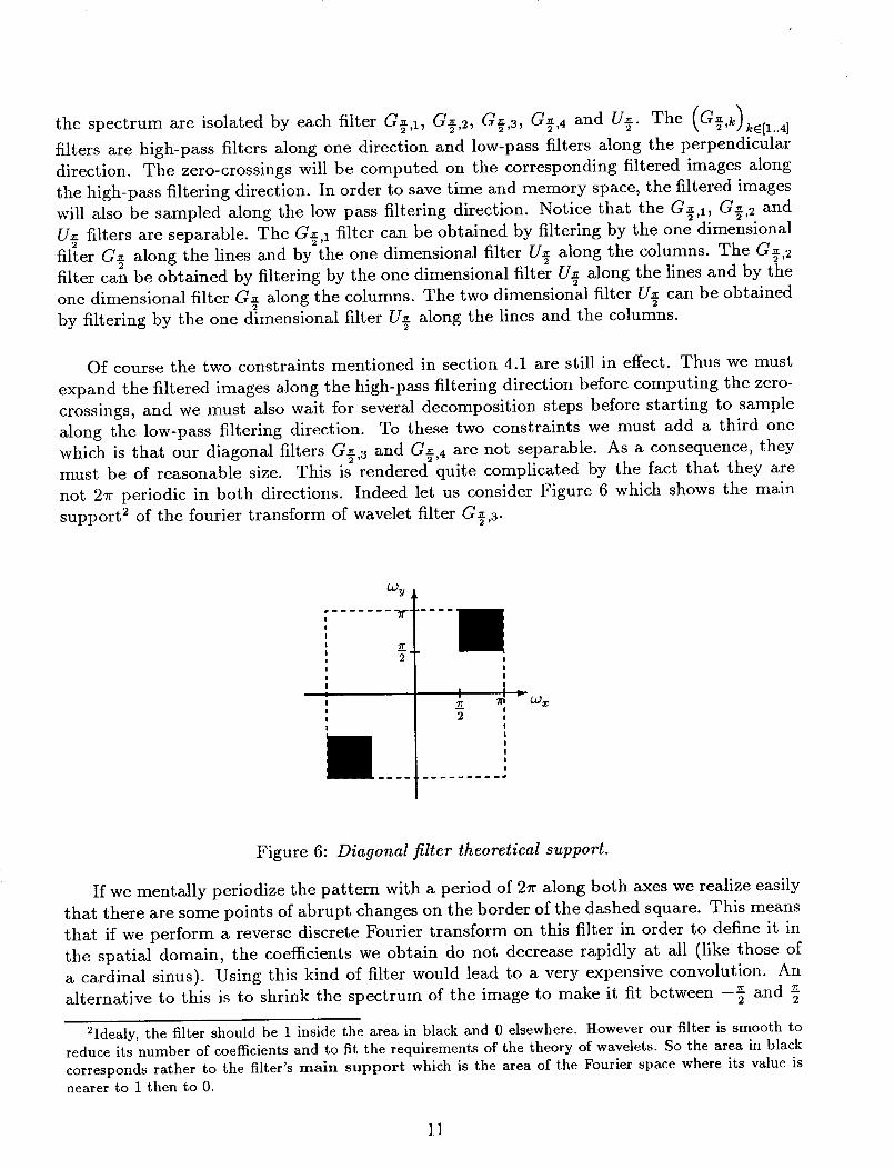
the spectrum are isolated by each filter G_,I, G_,2, G_,3, G_,4 and U_. The (G_,k)ke[1..41
filters are high-pass filters along one direction and low-pass filters along the perpendicular
direction. The zero-crossings will be computed on the corresponding filtered images along
the high-pass filtering direction. In order to save time and memory space, the filtered images
will also be sampled along the low pass filtering direction. Notice that the G-_,12, G_,2- and
U_ filters are separable. The G_,I filter can be obtained by filtering by the one dimensional
filter G_ along the lines and by the one dimensional filter U_ along the columns. The G_,2filter can be obtained by filtering by the one dimensional filter U_ along the lines and by the
one dimensional filter G-_ along the columns. The two dimensional filter U-_ can be obtained2 2
by filtering by the one dimensional filter U-_ along the lines and the columns.2
Of course the two constraints mentioned in section 4.1 are still in effect. Thus we must
expand the filtered images along the high-pass filtering direction before computing the zero-
crossings, and we must also wait for several decomposition steps before starting to sample
along the low-pass filtering direction. To these two constraints we must add a third one
which is that our diagonal filters G_,3 and G_,4 are not separable. As a consequence, theymust be of reasonable size. This is rendered quite complicated by the fact that they are
not 27r periodic in both directions. Indeed let us consider Figure 6 which shows the main
support 2 of the fourier transform of wavelet filter G_,a.
(.Oy
7r
2 II
I
] .
lr2
Figure 6: Diagonal filter theoretical support.
If we mentally periodize the pattern with a period of 2_r along both axes we realize easily
that there are some points of abrupt changes on the border of the dashed square. This means
that if we perform a reverse discrete Fourier transform on this filter in order to define it in
the spatial domain, the coefficients we obtain do not decrease rapidly at all (like those of
a cardinal sinus). Using this kind of filter would lead to a very expensive convolution. An
alternative to this is to shrink the spectrum of the image to make it fit between -3 and
2Idealy, the filter should be 1 inside the area in black and 0 elsewhere. However our filter is smooth toreduce its number of coefficients and to fit the requirements of the theory of wavelets. So the area in black
corresponds rather to the filter's main support which is the area of the Fourier space where its value is
nearer to 1 then to 0.
11
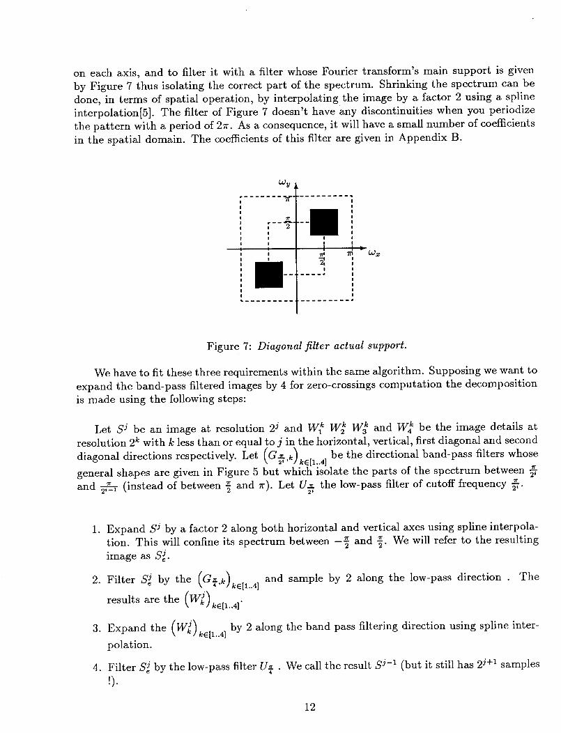
on each axis, and to filter it with a filter whose Fourier transform's main support is givenby Figure 7 thus isolating the correct part of the spectrum. Shrinking the spectrum can bedone, in terms of spatial operation, by interpolating the image by a factor 2 using a splineinterpolation[5]. The filter of Figure 7 doesn't have any discontinuities when you periodizethe pattern with a period of 2_r. As a consequence,it will have a small number of coefficientsin the spatial domain. The coefficients of this filter are given in Appendix B.
.......::}........._r
I
I
I
I
I
I
!
I I
!
Figure 7: Diagonal filter actual support.
We have to fit these three requirements within the same algorithm. Supposing we want to
expand the band-pass filtered images by 4 for zero-crossings computation the decomposition
is made using the following steps:
Let S j be an image at resolution 2 j and W k W k W3k and W4k be the image details at
resolution 2 k with k less than or equal to j in the horizontal, vertical, first diagonal and second
diagonal directions respectively. Let (G-_,k_ . . be the directional band-pass filters whose\ 2' ]kE[1..4]
general shapes are given in Figure 5 but which isolate the parts of the spectrum between 2--_
and _ (instead of between _ and r). Let U_, the low-pass filter of cutoff frequency #r.
1. Expand S j by a factor 2 along both horizontal and vertical axes using spline interpola-
tion. This will confine its spectrum between -_ and _. We will refer to the resulting
image as S j.
2. Filter S j by the (G_,k)ke[1..41 and sample by 2 along the low-pass direction. The
Jresults are the (W_)ke[1..41.
3. Expand the (W_)ke[1..4] by 2 along the band pass filtering direction using spline inter-
polation.
4. Filter S j by the low-pass filter U_ . We call the result S j-1 (but it still has 2 j+l samples
!).
12
5. Filter
resultS j-1 by the (G{,k)ke[1..4 ]
is the (W_ -1) ke[1..4]"
and sample by 4 along the low-pass direction . The
S j-1 by the low-pass filter U_ and sample by 2 along each axis . The result is
7. Filter
result
S j-2 by the (G.},k)ke[1..4 l
j--2
is the (W_)ke[1..4]"
and sample by 4 along the low-pass direction . The
8. Filter S j-2 by the low-pass filter U_ and sample by 2 along each axis . The result is
S j-3 and so on ...
In Appendix A we give the algorithm for an expansion factor of 2 instead of 4.
We can now compute the Energy-zero-crossings representation on the set of detail imagesi
(W_) (i,k) eli-: _..j] x [1..4] along the band-pass filtering directions. The integration we used methodfor energy computation is based on the spline interpolation and is exact for cubic spline
functions.
4.3 Energy-zero-crossings representation.
Let us consider the monodimensional case first, building an energy-zero-crossings represen-
tation from a dyadic wavelet representation consists in coding the detail signals not in terms
of pixels but in term of zero-crossings and energies between adjacent zero-crossings. Indeed
if the filters are properly chosen so as to make them proportional to the second derivative
of a smoothing function, the energy-zero-crossings representation directly points out to us
where the information is, and gives us a measure of the information's importance. The two
components of this representation are dealt with at different levels. First the detail signal is
transformed into a chained list of energy patches which are a representation of the energy
of each arch 3 of the signal. The information retained for each energy patch is the following:
• let S be the signal and x0 and xl two adjacent zero-crossings.
• let e be the energy of the arch between x0 and xl:
<= [S(x)12dx0
• let ¢ be the sign of S between x0 and xl.
3We call arch the portion of the signal between adjacent zero-crossings.
13

• let l the arch length defined by:
• let a be defined by:
l = x 1 - x0
al = 6c 2
• then a and l are the characteristic parameter describing the energy patch.
Then the signal representation looks like:
l
a
l
a
l
a
Figure 8: Energy list structure.
Having defined what an energy patch is we can now take the following structure for the
zero-crossings: A zero-crossing is defined by its abscissa, the energy patch on its right and
the energy patch on its left. All this is summarized in figure 9.
abscissa abscissa
r
1 l l
a a a
Figure 9: Energy-zero-crossings structure.
The two dimensional Energy-zero-crossings representation is a direct generalization on
the one-dimensional case. Each detail image has a band-pass filtering direction and a low-
pass filtering direction. We compute the energies and zero crossings along the band-pass
filtering direction treating these lines as one dimensional signals. For the (Wil)ie[j_n..j] the
zero-crossings are computed along the lines, for the (Wi2)ie[j_n..j] they are computed along the
14

columns, and for the (W_)ie[j_,..j ] (resp. (W_)ie[j__..j]) they are computed along the positive
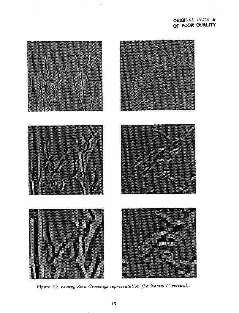
(resp. negative) diagonaP. Figure 10 shows the Energy-zero-crossings representation of the
dyadic decomposition of the image of Figure 13 (section 5.2) for the horizontal and vertical
orientations at the first three resolutions 2 j-l, 2 j-2 and 2 j-3.
4We call positive diagonal the diagonal that goes from bottom left to top right, and negative diagonalthe diagonal that goes from top left to bottom right
15
ORIGiNhL ' _ ""=
....... 1' Iiilr , -T :_:_ ......
........ +.+Figure 10: Energy-Zero-Crossings representation (horizontal _ vertical).
16
5 Completeness of the representations.
5.1 Dyadic wavelet transform.
Stephane Mallat has previously demonstrated that the dyadic wavelet transform was com-
plete for signals and images. However only the monodimensional simulation had been im-
plemented. In this paper we show results concerning a bidimensional implementation of the
dyadic reconstruction process. The reconstruction is based on the following property of the
U and G filters:
]G(w)[ 2 + [U(w)] 2 = 1
or, in two dimensions:4
Z 2 + 2 = 1i=1
This means that if S j is a signal and if we obtained S j-1 and W i by filtering by U and G
respectively, the original signal can be obtained by filtering S j-1 by U, by filtering W j by G
and by adding up the results. This is summarized in the following equation:
sj = S j-1, u + W j * g
Where u and g are the impulse responses of filters U and G. In fact this is not exactly true.
Indeed we must remember that we did certain operations of spline expansion and sampling
to obtain S j-1 and W j. Thus we must reverse these operations . The reverse of a spline
interpolation can be performed using a reduction/projection as shown by Stephane Mallat[1],
and the reverse of a decimation is an spline interpolation[5].
5.1.1 One dimensional algorithm.
We can now give the one dimensional reconstruction process. Supposing that we have de-
composed signal S j as described in Figure 2 and obtained W j, W j-l, W j-2, W j-3 and S j-4
we can reconstruct S j this way:
17
1. Expand S i-4 by a factor 2. The result is j-4S_xp •
j--42. Filter S_,p by U_.
3. Filter W j-3 by G_.
4. Add up the results. This gives S j-3.
_eXp "5. Expand S j-3 by a factor 2. The result is j-3
6. Filter sJ_-p3 by U_.
7. Filter W j-2 by G-_.8
8• Add up the results• This gives S j-2.
9. Filter S j-2 by U_•
10. Reduce W j-1 by a factor 2. The result is W_d 1
11. Filter W_d 1 by G_.
12. Add up the results. This gives SJ-I•
13. Filter S j-1 by U_•
14• Reduce W j by a factor 4• The result is w?_Jd
15. Filter w_.Jd by G-_.2
16• Add up the results. This gives S j.
5.1.2 Two dimensional algorithm.
For images, the algorithm is a little more complicated. The major obstacle to reconstruction
is the square grid. Let us first describe the basic steps. Supposing that we have decom-• j W j-1 W j-2posed signal S j and obtained the (W_ , ( , _ , (1 ,_ _ and S j-3 we can
\ "/kE[1..4] \ _ /kE[1..4] \ _ /kE[1..4]
reconstruct S j this way:
j--31. expand S j-3 by 2 along each axis. The result is S_p.
2. Expand the (W_-2)ke[1..4]
j-2the (W_pk )ke[1..4]"
by 4 along the low-pass filtering direction. The results are
( j-2) by the (G-_,k) . and sJ_-v3 by U__.3. Filter the W_p k ke[1..4] 8 kE[1..4] 8
18
4. Add up the results. This gives S j-2.
j--25. expand S j-2 by 2 along each axis. The result is Se,p-
6. Expand the (W_ -1) by 4 along the low-pass filtering direction. The results arek_[1..41
the (W_.p _--l)kE[,..4 I-
Seep by U-'.J-* (G_,k) ke[1..4] 87. Filter the (W_,p k )ke[1..4] by the and j-2
8. Add up the results, this gives S j-1.
9. Reduce the (W_)ke[,..4] by 2 along the band-pass filtering direction and expand them
by 2 along the low-pass filtering direction. The results are the (W_p {)ke[1..4]"
10. Filter the (W_,p {)ke[1..4] by the (G_,k)ke[1..41 and S j-1 by U_.
1 1. Add up the results, this gives S_j, which is S j expanded by a factor 2.
12. Reduce S j by 2 along each axis. This gives S j.
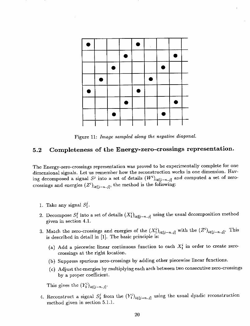
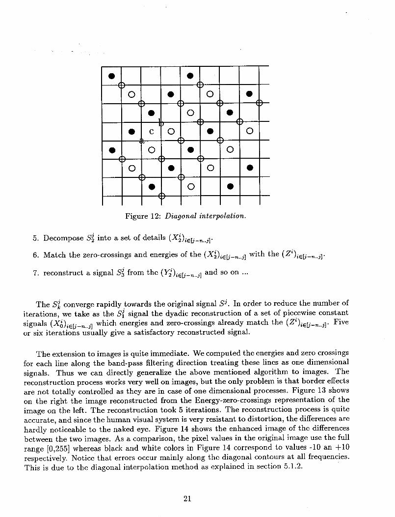
The critical steps here are steps 2, 6 and 9 for the images corresponding to the two
diagonal directions. These images have been obtained by sampling along the diagonal lines.
Due to the square shape of the pixels, it is very difficult to interpolate again along the
diagonal lines to reverse the sampling. The problem is that we have an array with only
certain diagonals containing pixels, and we want to fill in the empty pixels. Let us consider
an image sampled by four along the "negative" diagonal 5.
The process we have chosen is to interpolate by four along the negative diagonal, as
shown in Figure 12 (notice that the new pixels do not fit the square grid) and to fill in the
remaining empty pixels by linear interpolation along the positive diagonal. For example in
Figure 12, value at pixel "c" would be equal to the mean of value at pixel "a" and value at
pixel "b".
Of course this interpolation is not at all accurate since we perform a linear interpolation
--which is a rather poor interpolation-- along the direction containing the high frequencies.
However, this error appears only on the diagonal lines, for which the human visual system
has less sensitivity. Thus it is very difficult to detect this error except when looking at the
image of the differences between the original picture and the reconstructed picture.
5We call positive diagonal the diagonal that goes from bottom left to top right, and negative diagonal
the diagonal that goes from top left to bottom right
19
5.2
Figure 11: Image sampled along the negative diagonal.
Completeness of the Energy-zero-crossings representation.
The Energy-zero-crossings representation was proved to be experimentally complete for one
dimensional signals. Let us remember how the reconstruction works in one dimension. Hav-
ing decomposed a signal S j into a set of details (Wi)ie[j_,_..j] and computed a set of zero-
crossings and energies (zi)ie[j_n..j], the method is the following:
1. Take any signal S_.
2. Decompose S_ into a set of details i• (Xx)ie[/_...jl using the usual decomposition method
given in section 4.1.
i i(Z)_[J-_..Jl"3. Match the zero-crossings and energies of the (X1)ie[j_,..j I with the This
is described in detail in [1]. The basic principle is:
(a) Add a piecewise linear continuous function to each XI in order to create zero-
crossings at the right location.
(b) Suppress spurious zero-crossings by adding other piecewise linear functions.
(c) Adjust the energies by multiplying each arch between two consecutive zero-crossings
by a proper coefficient.
This gives the i
YJ4. Reconstruct a signal S_ from the ( 1)_e[j-_..j] using the usual dyadic reconstruction
method given in section 5.1.1.
2O
%
J
O
¢%
• 0 ••,j %J •J
• 0 •1 r_ t%
• c 0 • 0L •'% /'%%J %/
0 • 0
j •J _J
0 • 0 •/% g'%_,j %J
• 0 •¢%
Figure 12: Diagonal interpolation.
5. Decompose S_ into a set of details i
6. Match the zero-crossings and energies of the _ i(X2),e[j__..j] with the (Z)_e[j-_.d]"
7. reconstruct a signal S_ from the i(Y_)ie[j-_../] and so on ...
The S_ converge rapidly towards the original signal S j. In order to reduce the number of
iterations, we take as the S_ signal the dyadic reconstruction of a set of piecewise constant
(Z)ie[j-n..j]" Fivesignals i(X_)ie[j_,_..j] which energies and zero-crossings already match the i
or six iterations usually give a satisfactory reconstructed signal.
The extension to images is quite immediate. We computed the energies and zero crossings
for each line along the band-pass filtering direction treating these lines as one dimensional
signals. Thus we can directly generalize the above mentioned algorithm to images. The
reconstruction process works very well on images, but the only problem is that border effects
are not totally controlled as they are in case of one dimensional processes. Figure 13 shows
on the right the image reconstructed from the Energy-zero-crossings representation of the
image on the left. The reconstruction took 5 iterations. The reconstruction process is quite
accurate, and since the human visual system is very resistant to distortion, the differences are
hardly noticeable to the naked eye. Figure 14 shows the enhanced image of the differences
between the two images. As a comparison, the pixel values in the original image use the full
range [0,255] whereas black and white colors in Figure 14 correspond to values -10 an +10
respectively. Notice that errors occur mainly along the diagonal contours at all frequencies.
This is due to the diagonal interpolation method as explained in section 5.1.2.
21

ORIGINAL PAGE
BLACK AND WHITE PHOTOGt_APHPA_ •ORIGINAL "" _
OF POOl_ qu/u.,rrY
Figure 13: Original image and reconstruction from the Energy-Zero-Crossings representation.
Figure 14: Differences between the original image and its reconstruction.
22
6 Applications to higher level vision processes.
6.1 Edge detection.
The Energy-zero-crossings representation, together with the multiorientation feature, is a
useful model for edge finding algorithms. Indeed the zero-crossings point out where local
variations are and the energies give a measurement of the intensity of these variations.
Let us emphasize some terminology points here. It is important to define the meaning of
the word "direction" in what follows, supposing that we have applied a horizontal band-pass
filter and a vertical low-pass filter to an image, the direction of the edges we will look for
is the vertical direction (vertical edges are horizontal variations) thus we will refer to the
vertical direction as the main edge direction whereas we will call the image an image of
horizontal variations.
6.1.1 Basic edge-detection algorithm.
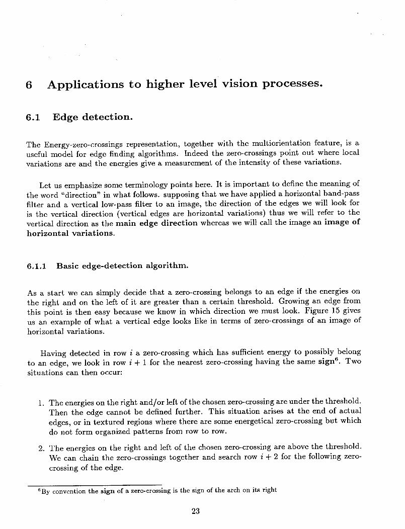
As a start we can simply decide that a zero-crossing belongs to an edge if the energies on
the right and on the left of it are greater than a certain threshold. Growing an edge from
this point is then easy because we know in which direction we must look. Figure 15 gives
us an example of what a vertical edge looks like in terms of zero-crossings of an image of
horizontal variations.
Having detected in row i a zero-crossing which has sufficient energy to possibly belong
to an edge, we look in row i + 1 for the nearest zero-crossing having the same sign 6. Two
situations can then occur:
1. The energies on the right and/or left of the chosen zero-crossing are under the threshold.
Then the edge cannot be defined further. This situation arises at the end of actual
edges, or in textured regions where there are some energetical zero-crossing but which
do not form organized patterns from row to row.
2. The energies on the right and left of the chosen zero-crossing are above the threshold.
We can chain the zero-crossings together and search row i + 2 for the following zero-
crossing of the edge.
6By convention the sign of a zero-crossing is the sign of the arch on its right
23
rew I * I
row I * 2
rawl _ $
Figure 15: Edge detection using zero-crossings.
This process is called edge-growing. Similarly we can investigate rows i - 1, i - 2
and so on to extend our edge. In our implementation, we have again used the zero-crossing
structure described in Figure 9 except that our zero-crossings are not linked along one line,
but between consecutive lines.
6.1.2 Algorithm improvement.
Of course this algorithm is far too simple to give satisfactory results. First of all, if we
use a single threshold, we often miss part of the edges we define due to contrast variations.However we must remember that we do not examine each zero-crossing independently to
decide whether or not it is part of an edge. Our approach is to look for zero-crossings which
would extend previously detected edges. Thus we use connectivity as a criterion. Having
realized that connectivity is part of the decision process, we can then reduce the threshold
constraint while growing the edge. So we now have two different thresholds. The first one is
used to detect starting points for our edge growing loop, and the other one, which is weaker,
is used while actually growing the edges.
The next technical problem is that although now we can detect connected "chains" of
zero-crossings, not all these chains correspond to actual edges in the image. The reason for
this is the following: The theory of wavelet provides us with a large class of possible filters.
We then put some requirements for the filter we choose:
• It has to be proportional to the second derivative of a smoothing function, so that the
zero-crossings mark inflection points.
24
• It has to be localized in spaceso that we can accurately locate these inflection points.This is also important for computation speed.
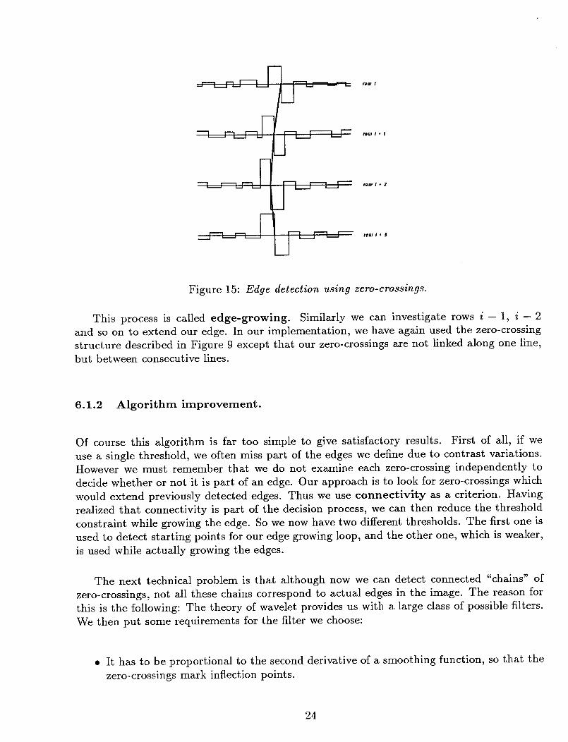
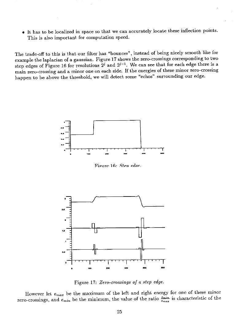
The trade-off to this is that our filter has "bounces", instead of being nicely smooth like forexample the laplacian of a gaussian. Figure 17showsthe zero-crossingscorresponding to twostep edgesof Figure 16 for resolutions 2 j and 2 j-1. We can see that for each edge there is a
main zero-crossing and a minor one on each side. If the energies of these minor zero-crossing
happen to be above the threshold, we will detect some "echos" surrounding our edge.
l--
o.a
o.a --
o.4 --
o .... I .... I .... I ....... I10o soo _ _o rJoo
FiCnre lfi: ,qten edae.
3_
2.6
2_
1.6
O,C
0
p \
..... I .... I .... I .... I .... I0 100 200 300 400 600
Figure 17: Zero-crossings of a step edge.
However let em_ be the maximum of the left and right energy for one of these minor
zero-crossings, and emi_ be the minimum, the value of the ratio _._x is characteristic of the
25

edge type. If this edge is an echo, this ratio is usually 15 to 20 % depending on the filter we
chose, whereas for real edges, its value is above 40 %. This is a simple way of discriminating
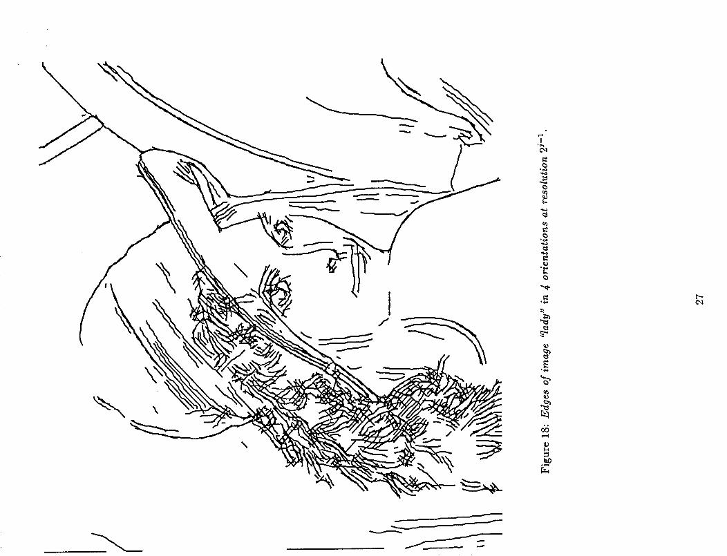
echo edges from actual ones. Figure 18 and Figure 19 shows the edges of the image in
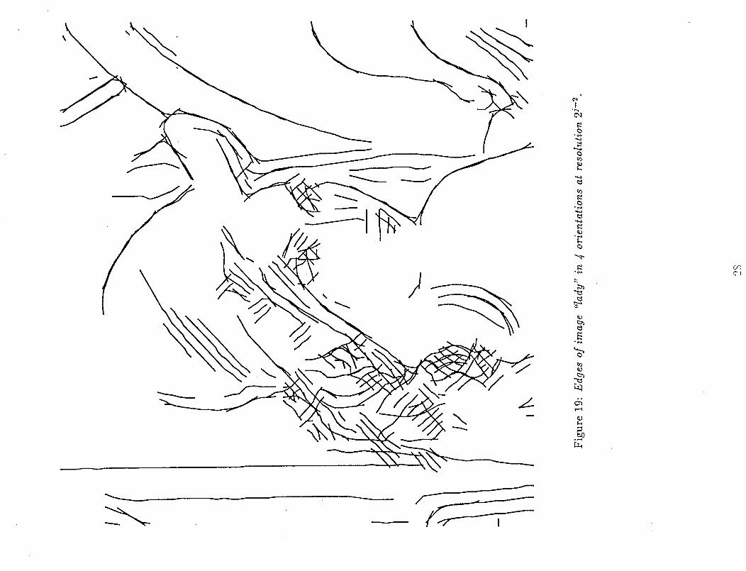
Figure 13 as they appear at resolutions 2 j and 2j-1. Notice that some edges are redundant
whereas some appear only at a the coarser or finer resolution. Notice also that the junction
between orientations is smooth if the actual edge is spatially smooth (i.e. if its curvature is
small).
26
A _,o
r
f
\
\J
q.)_b
°L.._
q_
o_
c_
%
\
C_t
I°_.._
qh_
°Lk_
o_
Q_
@

• ,:..
6.1.3 Edge finding and multiorientation.
It is possible that an edge will appear on several images corresponding to different orientation.
Indeed we chose filters that were localized in the spatial domain. As a consequence, their
cut-off capacities were smothered in the frequency domain. This causes the filters to overlap
both between orientations and resolutions. For example if while looking for vertical edges
we detect an edge which is bent 30 ° from the vertical, there are great chances that this edge
will also be detected by looking at the zero-crossings of the image of diagonal variations. In
fact we can control the amount of redundancy by including constraints on the direction in
the edge-growing algorithm. For example we can stop growing the edge if the next potential
segment happens to make an angle of more than 30 ° with the main edge direction, as we
expect it to be detected in another orientation anyway. This is important because we might
want to build algorithms which link continuous segments, such as circles, having some parts
in different orientations.
6.2 Corner detection.
As stated in section 3 if we use a pattern recognition process based on image decomposition
and recomposition, multiorientation is a definite advantage for the detection of interesting
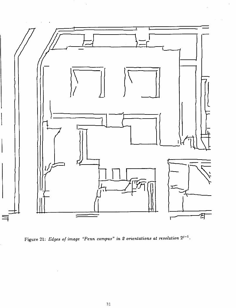
structural points like corners, "T" junctions and so on. Figure 21 shows the horizontal and
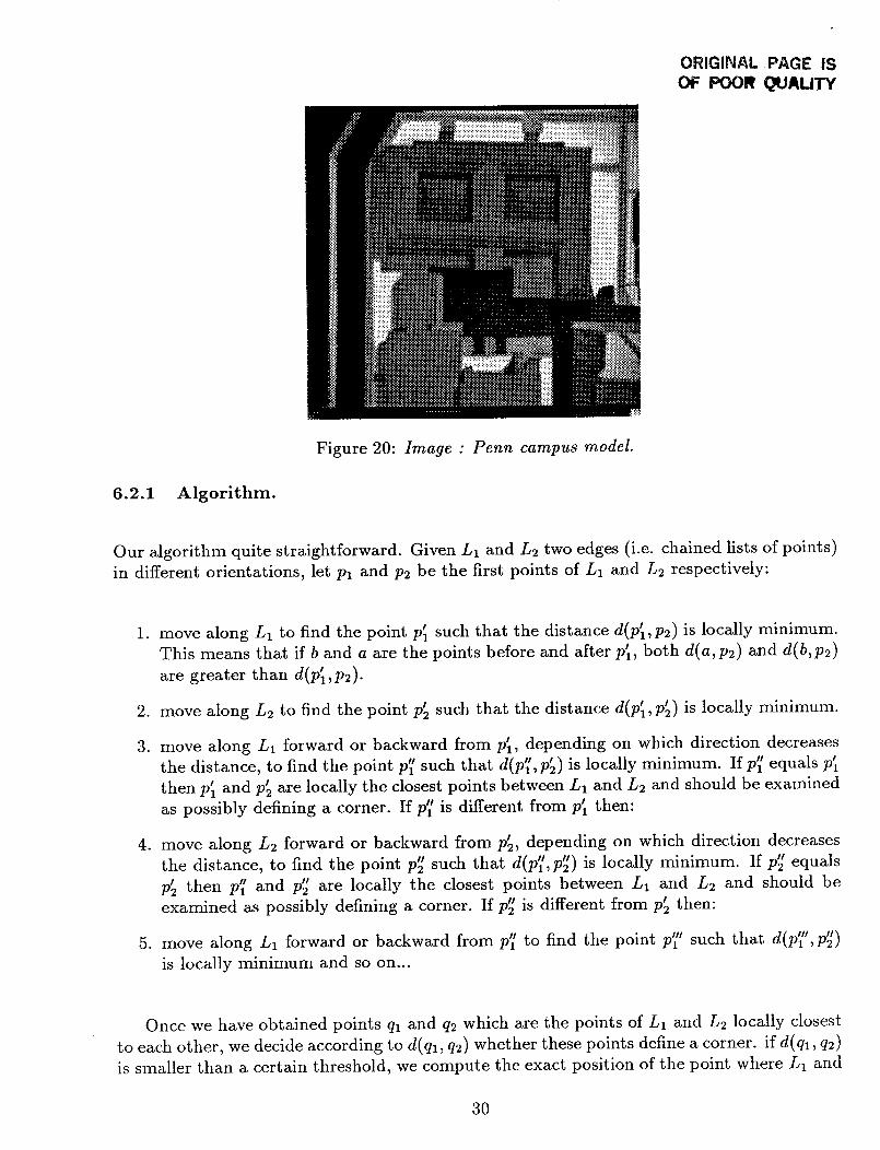
vertical edges of the image in Figure 20 representing a model of the Penn campus. It shows
that the corners are not affected by our edge detection method. All we have to do is to take
edges within two different orientations and to look for crossing points.
The wavelet filters are localized enough to prevent ambiguities on corner detection. More-
over, we can get accurate information about the tangents at the corner location. These corner
points are relevant to the image understanding for several reasons. First of all, corners are
usually the points of an object's contour which are the most useful to define it's geometry.
For example, it much easier to detect motion by observing the corners than by trying to
match edges. Also corner points are generally points of interaction between several objects
in the scene. A "T" junction for example is a point which which plays a role in the definition
of three different objects or regions, so there is a lot of information associated to such a
point. Another reason is that unconnected edges very seldomly exist in real scenes. Or if
these exist, they often correspond to a lack of information we should take care of. The best
example of this are illusory contours. The human visual system reacts to illusory patterns
by mentally adding some edge portions to incomplete segments so as to try to define a rec-
ognizable shape. If we want to detect unconnected edge segments for further analysis, it
is a good idea to first detect edges which are connected by corners, then to deal with the
remainder.
29
ORIGINAL PAGE IS
OF POOR qUAUTY
Figure 20: Image : Penn campus model.
6.2.1 Algorithm.
Our algorithm quite straightforward. Given L1 and L2 two edges (i.e. chained lists of points)
in different orientations, let Pl and p2 be the first points of L1 and L2 respectively:
°
,
3.
.
.
move along L1 to find the point p_ such that the distance d(p'l,p2 ) is locally minimum.
This means that if b and a are the points before and after p_, both d(a,p2) and d(b, p2)
are greater than d(p_,p2).
move along L2 to find the point p_ such that the distance d(p'x, P'2) is locally minimum.
move along L1 forward or backward from p_, depending on which direction decreasesII II I Ithe distance, to find the point Pl such that d(Pl, P2) is locally minimum. If p_ equals Pl
then p_ and p_ are locally the closest points between L1 and L2 and should be examined
as possibly defining a corner. If p_' is different from p_ then:
move along L2 forward or backward from p_, depending on which direction decreases
the distance, to find the point p_ such that d(p'_', p'_) is locally minimum. If p_ equals
p_ then p_ and p_ are locally the closest points between L1 and L2 and should be
examined as possibly defining a corner. If p_ is different from p_ then:
move along L, forward or backward from p_ to find the point p_" such that d(p'a", p_)
is locally minimum and so on...
Once we have obtained points ql and q2 which are the points of L1 and L2 locally closest
to each other, we decide according to d(ql, q2) whether these points define a corner, if d(ql, q2)
is smaller than a certain threshold, we compute the exact position of the point where L1 and
3O
m
I
i l
\/
I
J
I
II
I
Figure 21: Edges of image "Penn campus" in 2 orientations at resolution 2 j-1.
31
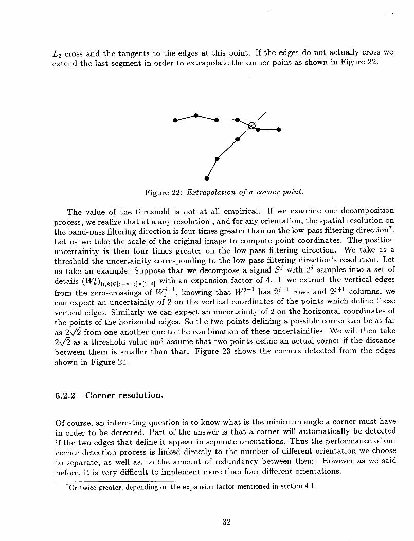
L2 cross and the tangents to the edges at this point. If the edges do not actually cross we
extend the last segment in order to extrapolate the corner point as shown in Figure 22.
Figure 22: Extrapolation of a corner point.
The value of the threshold is not at all empirical. If we examine our decomposition
process, we reMize that at a any resolution, and for any orientation, the spatial resolution on
the band-pass filtering direction is four times greater than on the low-pass filtering direction 7.
Let us we take the scale of the original image to compute point coordinates. The position
uncertainity is then four times greater on the low-pass filtering direction. We take as a
threshold the uncertainity corresponding to the low-pass filtering direction's resolution. Let
us take an example: Suppose that we decompose a signal S j with 2 j samples into a set of
details (W_)(_,k)e[j_,_..j]×[1..4 ] with an expansion factor of 4. If we extract the vertical edges
from the zero-crossings of W j-l, knowing that W j-1 has 2 j-1 rows and 2 j+l columns, we
can expect an uncertainity of 2 on the vertical coordinates of the points which define these
vertical edges. Similarly we can expect an uncertainity of 2 on the horizontal coordinates of
the points of the horizontal edges. So the two points defining a possible corner can be as far
as 2v/2 from one another due to the combination of these uncertainities. We will then take
2x/_ as a threshold value and assume that two points define an actual corner if the distance
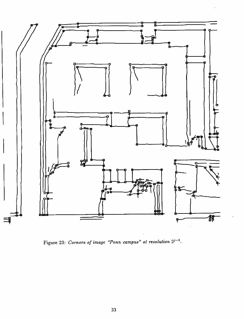
between them is smaller than that. Figure 23 shows the corners detected from the edges
shown in Figure 21.
6.2.2 Corner resolution.
Of course, an interesting question is to know what is the minimum angle a corner must have
in order to be detected. Part of the answer is that a corner will automatically be detected
if the two edges that define it appear in separate orientations. Thus the performance of our
corner detection process is linked directly to the number of different orientation we choose
to separate, as well as, to the amount of redundancy between them. However as we said
before, it is very difficult to implement more than four different orientations.
7Or twice greater, depending on the expansion factor mentioned in section 4.1.
32
\/ i
I
!
II
!
Figure 23: Corners of image "Penn campus" at resolution 2 j-:.
33
An alternative could be to use only one separable filter corresponding to a horizontal
band-pass filter and a vertical low pass filter, for example, and to apply it to several rotation
interpolations of the original image. Of course while performing the rotation interpolation
we will loose high frequencies. However we can still perform edge and corner detection at
all resolutions except the first one.
6.3 Unconnected lines detection: an example of feed-back.
As stated earlier, unconnected line segments occur very seldom in natural scenes. However,
many edge detectors which are not based on region growing, including ours, fail to connect
some edges. Knowing that unconnected patterns are very unlikely, we can localize the areas
where our edge detection process gives incomplete results, and tune the process differently
in those areas. Also, we have the alternative of using different methods for this particular
image portion such as using another picture with a different lighting condition, or artificially
enhancing the contrast.
Detecting edges with loose ends is done simply by looking at the two ends of each edge
and to see whether they have been used to define corners. If either of them is not, it is
considered as loose end. As we now try to make an adaptive process by locally tuning the
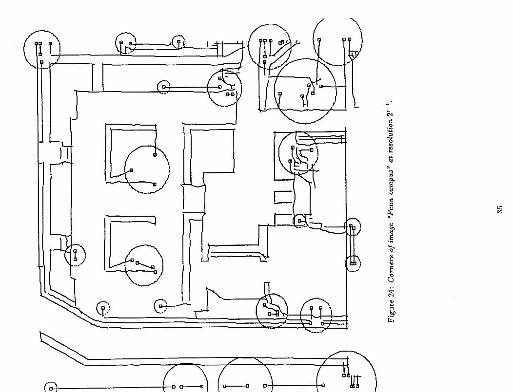
parameter of our edge detector, it is useful to regroup these loose end points into clusters.
This way we can apply some feed back at different levels. Either we change the image
acquisition system in the area corresponding to a particular cluster, or we locally change the
threshold and try to extend and connect the lines within a cluster. The clustering algorithm
is based on the minimum spanning tree computation and is given in Appendix C. Results
are shown in Figure 24. The circled area correspond to regions where the edges are generally
less obvious.
A Dyadic decomposition with an expansion by 2.
A.1 One dimensional algorithm.
Let S j be a signal at resolution 2 j and W j be the signal of the differences between S j and
S j-1. Let U#, be the low-pass filter with a cutoff frequency of _ and G__2, be the high-pass
(W)ie[j-_..j] by afilter with a cutoff frequency of _. supposing that we want to expand the i
factor 2 the algorithm is:
1. Filter S j by G_ . The result is W j
2. Expand W j by a factor 2
34
@
®
E3t-mo j • o i
• t,, a
o_,_
Q_
EC
c_
3. Filter S 3 by U_ . The result is S j-1 (but it still has 2 j samples I)
4. Filter S j-1 by G_ . The result is W j-1
5. Filter S j-1 by U_ and sample by 2. The result is S j-2
6. Filter S j-2 by G_ . The result is W j-2
7. Filter S j-e by U_ and sample by 2. The result is S j-3
8. Filter S j-3 by G_ . The result is W j-3
9. Filter S j-3 by U_ and sample by 2. The result is S j-4 and so on...
A.2 Two dimensional algorithm.
Let S j be an image at resolution 2 j and W k W k W3k and W k be the image details at resolution
2 k with k inferior or equal to j iy the horizontal, vertical, first diagonal and second diagonaldirections respectively. Let (Gv,k) ke[1..4] be the directional band-pass filters whose general
shapes are given in Figure 5 but which isolate the parts of the spectrum between _ and
(instead of between _ and _r). Let U_ the low-pass filter of cutoff frequency _.
Filter
result
Filter
S J-2.
Filter
result
1. Expand S j by a factor 2 along both horizontal and vertical axes using spline interpola-
tion. This will confine its spectrum between -3 and 3" We will refer to the resulting
image as Sej.
2. Filter S_j by the ( _, )ke[1..4lG-k and sample by 2 along the low-pass direction. The
results are the (W_)ke[1..4]"
3. Filter S j by the low-pass filter U} and sample by 2 along each axis . The result is S j-1
(but it has 2 j samples).
4. S j-1 by the (G--k) and sample by 4 along the low-pass direction . The4' kE[1..4]
j-1is
5. S j-1 by the low-pass filter U_ and sample by 2 along each axis . The result is
6. S j-2 by the ( _ )ke[1..4lG-,k and sample by 4 along the low-pass direction . The
is the (W_ -2) ke[1..41"
7. Filter S j-2 by the low-pass filter U_ and sample by 2 along each axis . The result is
S j-3 and so on ...
36
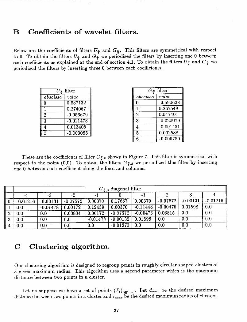
B Coefficients of wavelet filters.
Below are the coefficients of filters U-- and G-_. This filters are symmetrical with respect2 2
to 0. To obtain the filters U-_ and G-- we periodized the filters by inserting one 0 between4 4
each coefficients as explained at the end of section 4.1. To obtain the filters U_ and G_ we
periodized the filters by inserting three 0 between each coefficients.
U_ filter
abscissa valu e
0 0.587132
1 0.274067
2 -0.056679
3 -0.021478
4 0.013405
5 -O.O03085
Ga filter
abscissa value
0 -0.590628
1 0.267548
2 0.047401
3 -0.020079
4 -0.001451
5 O.O02588
6 -0.000750
These are the coefficients of filter G},3 shown in Figure 7. This filter is symmetrical with
respect to the point (0,0). To obtain the filters G_,3 we periodized this filter by inserting
one 0 between each coefficient along the lines and columns.
0
1
2
3
4
G_,3 diagonal filter-4 -3 -2 -1
-0.01216 -0.00131 -0.07572 0.00370 0.17657 0.00370 -0.07572 -0.00131 -0.01216
0.0 -0.01478 0.00172 0.12439 0.00370 -0.11448 -0.00476 0.01598 0.0
0.0 0.0 0.03834 0.00172 -0.07572 -0.00476 0.03815 0.0 0.0
0.0 0.0 0.0 -0.01478 -0.00132 0.01598 0.0 0.0 0.0
0.0 0.0 0.0 0.0 -0.01273 0.0 0.0 0.0 0.0
-1 4
C Clustering algorithm.
Our clustering algorithm is designed to regroup points in roughly circular shaped clusters of
a given maximum radius. This algorithm uses a second parameter which is the maximum
distance between two points in a cluster.
Let us suppose we have a set of points (Pi)iE[1..n ]. Let dm_, be the desired maximumdistance between two points in a cluster and rm_ be the desired maximum radius of clusters.
37
The algorithm is the following:
1. Compute the minimum spanning tree of the (Pi)ie[1..n]" The result is a set of arcs
(Ai)_e[1...q"
2. Remove every arc greater than dm_. This yields several sub-trees. Points which belongto the same sub-tree form a cluster. The result is thus a set of clusters (C!°)_
\ t /iE[1..k0]
3. For each cluster C (°) compute the center of gravity gi of all the points in it , then
compute the distances between gi and each point in the cluster. Let ri be the maximum
of these distances.
4. For each cluster C_ °), if ri is greater than rm_ then break the longest arc of the
corresponding sub-tree. This yields two "sub-subtrees" defining two sub-clusters C! 1)
and C} 2).
5. Repeat the two previous steps on the C} j) until no further subdivision occurs. The
result is a set of clusters Ci fulfilling the desired requirements.
References
[1] Stephane Mallat. Multiresolution Representations and Wavelets. PhD thesis, University
of Pennsylvania, Department of Computer and Information Science, School of Engineer-
ing and Applied Science, August 1988.
[2] Stephane Mallat. Dyadic wavelet energy zero-crossings. Technical Report MS-CIS-88-30,
University of Pennsylvania, Department of Computer and Information Science, School of
Engineering and Applied Science, 1988. To appear as an invited paper in IEEE Trans.
on Information Theory.
[3]
[4]
[5]
[6]
Eric p. Krotkov. Results in finding edges and corners in images using the first directionnal
derivative. Technical Report MS-CIS-85-14, University of Pennsylvania, Department of
Computer and Information Science, School of Engineering and Applied Science, March
1985.
F. Campbell and J. Kulikowski. Orientation selectivity of the human visual system.
Journal of Physiology, 197:437-441, 1966.
R. C. Crochiere and L. R. Rabiner. Interpolation and decimation in signal processing.
Proceeding on the IEEE, 69, March 1981.
Philip J. Davis and Philip Rabinowitz. Methods of Numerical Integration, chapter 2.3.1,
page 62. Computer Science and Applied Mathematics, 19??
38

List of Figures
1 Conceptual process .................................
82 Real process .....................................
3 Low pass filter U_ ................................. 9
4 Low pass filter U_ periodized by 2 ......................... 10
5 Splitting of the spectrum using wavelet filters .................. 10
6 Diagonal filter theoretical support ......................... 11
7 Diagonal filter actual support ........................... 12
8 Energy list structure ................................ 14
9 Energy-zero-crossings structure .......................... 14
10 Energy-Zero-Crossings representation (horizontal _ vertical) .......... 16
11 Image sampled along the negative diagonal .................... 20
12 Diagonal interpolation ............................... 21
13 Original image and reconstruction from the Energy-Zero-Crossings represen-
tation ........................................ 22
14 Differences between the original image and its reconstruction .......... 22
15 Edge detection using zero-crossings ........................ 24
16 Step edge ...................................... 25
17 Zero-crossings of a step edge ........................... 25
18 Edges of image "lady" in _, orientations at resolution 2 j-1 ........... 27
19 Edges of image "lady" in _ orientations at resolution 2 j-2 ........... 28
39

20 Image : Penn campus model ............................
21 Edges of image "Penn campus" in 2 orientations at resolution 2 j-1 ......
22 Extrapolation of a corner point ..........................
23 Corners of image "Penn campus" at resolution 2 j-1 ..............
24 Corners of image "Penn campus" at resolution 2 j-1 ..............
3O
31
32
33
35
4O