Embed Size (px)
Citation preview
HAL Id: tel-03263863https://tel.archives-ouvertes.fr/tel-03263863
Submitted on 17 Jun 2021
HAL is a multi-disciplinary open accessarchive for the deposit and dissemination of sci-entific research documents, whether they are pub-lished or not. The documents may come fromteaching and research institutions in France orabroad, or from public or private research centers.
L’archive ouverte pluridisciplinaire HAL, estdestinée au dépôt et à la diffusion de documentsscientifiques de niveau recherche, publiés ou non,émanant des établissements d’enseignement et derecherche français ou étrangers, des laboratoirespublics ou privés.
Imaging for scattering properties of the crust : body tosurface waves couplingAndres Camilo Barajas Ramirez
To cite this version:Andres Camilo Barajas Ramirez. Imaging for scattering properties of the crust : body to sur-face waves coupling. Earth Sciences. Université Grenoble Alpes [2020-..], 2021. English. NNT :2021GRALU012. tel-03263863
THÈSEPour obtenir le grade de
DOCTEUR DE L’UNIVERSITÉ GRENOBLE ALPESSpécialité : Sciences de la Terre et de l'Univers et de l'EnvironnementArrêté ministériel : 25 mai 2016
Présentée par
Andres BARAJAS
Thèse dirigée par Michel CAMPILLO, Professeur et codirigée par Ludovic MARGERIN, DR CNRS, Université Toulouse III - Paul Sabatier
préparée au sein du Laboratoire Institut des Sciences de la Terredans l'École Doctorale Sciences de la Terre de l'Environnement et des Planètes
Imagerie des propriétés de diffraction: le couplage entre ondes de volume et de surface
Imaging for scattering properties of the crust: body to surface waves coupling
Thèse soutenue publiquement le 15 mars 2021,devant le jury composé de :
Monsieur Michel CAMPILLOPROFESSEUR DES UNIVERSITES, UGA, Directeur de thèseMonsieur Ludovic MARGERINDIRECTEUR DE RECHERCHE, CNRS, Co-directeur de thèseMonsieur Haruo SATOPROFESSEUR EMERITE, Tohoku University, RapporteurMonsieur Christoph SENS-SCHöNFELDERPROFESSEUR ASSISTANT, German Research Centre for Geosciences GFZ, Potsdam, RapporteurMadame Anne PAULDIRECTEUR DE RECHERCHE, CNRS, PrésidenteMonsieur German PRIETOPROFESSEUR ASSOCIE, Universidad Nacional de Colombia, Examinateur

i
Abstract
The analysis of the ambient seismic noise has proven to be a powerful tool to assessvelocity changes within Earth’s crust using coda-wave interferometry (CWI). CWI is basedon the analysis of small waveform changes in the coda of the signals, which can give usinformation about the structure or dynamic of the internal layers of the earth. The objectiveof this thesis is to separate and locate at depth the source of these changes. The work herepresented is developed in three main stages:
First, we aim to disentangle the processes behind velocity changes detected from a ten-year-long recording of seismic noise made with a single station in the region of Pollino, in thesouth of Italy. This region is characterized by the presence of aquifers and by a relatively shortperiod of high seismic activity which includes aM5.0 earthquake that occurred on the 25th ofOctober 2012. We apply two models that estimate the water level inside the aquifer makinga good prediction of the measured apparent δv/v which means that the velocity variation isdriven by changes in the pore pressure inside the aquifer. A parallel independent confirmationis obtained with geodetic measurements that show a volumetric expansion of the zone thatfollows the same patterns observed in the models and the velocity variation. The subtractionof these patterns from the measurements reveals a weak elastic response of the crust to therainfall and unravels the stress drop produced by the seismic event.
Second, we turn to the problem of localizing and imaging the source that generates thechanges at depth in the waveform registered at the surface. For this, we use a 3-D wave scalarmodel that couples naturally body and surface waves. Based on this model we make importantdeductions of the physical characteristics of the system like a depth-dependent body-to-surfacemean free path and a progressive energy transformation from surface to body waves. Usingthe radiative transfer equations that describe this system we perform a series of Monte-Carlosimulations to estimate the sensitivity kernel. We analyze its most important features andfind a good agreement when we compare it with other studies that use full wavefield numericalsimulations and independent surface and body wave sensitivities to estimate the sensitivity ofthe system. We also find that the ratio between the surface wave penetration and the meanfree path completely determines the evolution of the system, a feature not seen in previousstudies.
Finally, we study the process of locating the sources using the sensitivity kernel and aseries of observations: the inversion problem. We design a series of synthetic tests to assessthe capacity of the inversion to retrieve a velocity perturbation in different scenarios thatinvolve the depth of the perturbation in the medium, the duration of the coda used in theinversion, and the level of noise in the system. We make a first application of the inversionfor the case study in Italy and analyze its most relevant characteristics.

iii
Résumé
L’analyse du bruit sismique ambiant s’est avérée être un puissant outil pour évaluer les chan-gements de vitesse au sein de la croûte terrestre à l’aide de l’interférométrie par onde de coda(CWI). La CWI est basée sur l’analyse des petites variations de forme d’onde dans la codades signaux, ce qui peut nous donner des informations sur la structure ou la dynamique descouches internes de la terre. L’objectif de cette thèse est de séparer et de localiser en pro-fondeur la source de ces changements. Le travail présenté ici est développé en trois étapesprincipales :
Premièrement, nous cherchons à dissocier les processus à l’origine des changements devitesse dans la région de Pollino, dans le sud de l’Italie. Pour cela, nous utilisons un enregis-trement de bruit sismique continu d’une durée de dix ans avec une seule station. Cette régionest caractérisée par la présence d’aquifères et par une période relativement courte de forteactivité sismique, dont un tremblement de terre de M5 qui s’est produit le 25 octobre 2012.Nous appliquons deux modèles qui estiment le niveau de l’eau dans l’aquifère permettantune bonne prédiction du δv/v apparent mesuré, ce qui signifie que la variation de vitesse estdue aux changements de la pression interstitielle à l’intérieur de l’aquifère. Une confirmationparallèle indépendante est obtenue avec des mesures géodésiques qui montrent une expansionvolumétrique de la zone qui suit les mêmes patterns que ceux observés dans les modèles etla variation de vitesse. La soustraction de ces modèles de mesures révèle une faible réponseélastique de la croûte aux précipitations et met en évidence la chute de contrainte produitepar l’événement sismique.
Ensuite, nous abordons le problème de la localisation et de l’imagerie de la source quigénère les changements en profondeur dans la forme d’onde enregistrée à la surface. Pourcela, nous utilisons un modèle scalaire d’onde 3D qui couple naturellement les ondes de vo-lume et de surface. Sur la base de ce modèle, nous faisons d’importantes déductions sur lescaractéristiques physiques du système comme : un libre parcours moyen des ondes de volumeavant qu’elles ne se transforment en ondes de surface dépendant de la profondeur ; et unetransformation progressive de l’énergie des ondes de surface vers celles de volume. En utili-sant les équations de transfert radiatif qui décrivent ce système, nous effectuons une série desimulations de Monte-Carlo pour estimer le noyau de sensibilité. Nous analysons ses caracté-ristiques les plus significatives et trouvons une bonne concordance lorsque nous le comparonsavec d’autres études qui utilisent des simulations numériques du champ d’onde complet et dessensibilités indépendantes des ondes de surface et de volume pour estimer la sensibilité dusystème. Nous constatons également que le rapport entre la pénétration des ondes de surfaceet le libre trajet moyen détermine entièrement l’évolution du système, une caractéristique nondétectée dans les précédentes études.
Enfin, nous étudions le processus de localisation des sources en utilisant le noyau desensibilité et une série d’observations : le problème inverse. Nous concevons une série detests synthétiques pour évaluer la capacité de l’inversion à retrouver une perturbation devitesse dans différents scénarios qui impliquent la profondeur de la perturbation dans le milieu,la durée de la coda utilisée dans l’inversion et le niveau de bruit dans le système. Nous

iv
faisons une première application de l’inversion pour l’étude de cas en Italie et analysons sescaractéristiques les plus pertinentes.
v
Acknowledgements
• Thanks to my jury members, Haruo Sato and Christoph Sens-Schönfelder, who atten-tively read my manuscript, and Anne Paul and German Prieto for their interest in ourwork.
• Thanks to my two thesis directors, Ludovic Margerin and Michel Campillo, for theopportunity to participate in this exciting project and for all the things they taught mealong the way.
• Thanks to the wave team and especially to Léonard Seydoux, Piero Poli, and Qing-YuWang for all their support during my Ph.D.
• Thanks to all the wonderful community at Isterre for making my time at Grenoble anunforgettable period of my life.
• Thanks to my parents and family for all their support from the distance.
• Thanks to Estelle for the interesting discussions, for her love, and especially for all thesupport during the writing of this thesis.


vii
Contents
Abstract i
Acknowledgements v
1 Introduction 1
2 Concepts and methods 32.1 Radiative transfer theory . . . . . . . . . . . . . . . . . . . . . . . . . . . . . . 3
2.1.1 Radiative transfer equation . . . . . . . . . . . . . . . . . . . . . . . . 42.1.2 Diffusion approximation . . . . . . . . . . . . . . . . . . . . . . . . . . 5
2.2 Equipartition of the energy . . . . . . . . . . . . . . . . . . . . . . . . . . . . 72.3 Coda wave interferometry . . . . . . . . . . . . . . . . . . . . . . . . . . . . . 7
2.3.1 MCSW method . . . . . . . . . . . . . . . . . . . . . . . . . . . . . . . 82.4 Seismic interferometry . . . . . . . . . . . . . . . . . . . . . . . . . . . . . . . 9
2.4.1 Passive image interferometry . . . . . . . . . . . . . . . . . . . . . . . 112.5 Sensitivity kernels . . . . . . . . . . . . . . . . . . . . . . . . . . . . . . . . . 12
2.5.1 Observation and motivation . . . . . . . . . . . . . . . . . . . . . . . . 122.5.2 Basic theory of traveltime sensitivity kernels . . . . . . . . . . . . . . . 14
3 Separation of phenomena from δv/v measurements 193.1 Abstract . . . . . . . . . . . . . . . . . . . . . . . . . . . . . . . . . . . . . . . 193.2 Introduction . . . . . . . . . . . . . . . . . . . . . . . . . . . . . . . . . . . . . 203.3 Data processing description . . . . . . . . . . . . . . . . . . . . . . . . . . . . 213.4 Procedure and results . . . . . . . . . . . . . . . . . . . . . . . . . . . . . . . 23
3.4.1 Measured and modeled velocity variations . . . . . . . . . . . . . . . . 233.4.2 Analysis of geodetic data . . . . . . . . . . . . . . . . . . . . . . . . . 27
3.5 Loading effect of the rainfall . . . . . . . . . . . . . . . . . . . . . . . . . . . . 303.6 Conclusions . . . . . . . . . . . . . . . . . . . . . . . . . . . . . . . . . . . . . 313.7 Supplementary information . . . . . . . . . . . . . . . . . . . . . . . . . . . . 34
4 Coupling between surface and body waves 434.1 Abstract . . . . . . . . . . . . . . . . . . . . . . . . . . . . . . . . . . . . . . . 434.2 Introduction . . . . . . . . . . . . . . . . . . . . . . . . . . . . . . . . . . . . . 444.3 Scalar wave equation model with surface and body waves . . . . . . . . . . . 46
4.3.1 Equation of motion . . . . . . . . . . . . . . . . . . . . . . . . . . . . . 464.3.2 Eigenfunctions and Green’s function . . . . . . . . . . . . . . . . . . . 474.3.3 Source radiation and density of states . . . . . . . . . . . . . . . . . . 50
4.4 Single scattering by a point scatterer . . . . . . . . . . . . . . . . . . . . . . . 524.4.1 Scattering of a surface wave . . . . . . . . . . . . . . . . . . . . . . . . 524.4.2 Scattering of body waves . . . . . . . . . . . . . . . . . . . . . . . . . . 53
4.5 Equation of radiative transfer . . . . . . . . . . . . . . . . . . . . . . . . . . . 554.5.1 Phenomenological derivation . . . . . . . . . . . . . . . . . . . . . . . 55

viii
4.5.2 Energy conservation and equipartition . . . . . . . . . . . . . . . . . . 574.5.3 Diffusion Approximation . . . . . . . . . . . . . . . . . . . . . . . . . . 59
4.6 Monte-Carlo Simulations . . . . . . . . . . . . . . . . . . . . . . . . . . . . . . 614.6.1 Overview of the method . . . . . . . . . . . . . . . . . . . . . . . . . . 614.6.2 Numerical results . . . . . . . . . . . . . . . . . . . . . . . . . . . . . . 62
4.7 Conclusions . . . . . . . . . . . . . . . . . . . . . . . . . . . . . . . . . . . . . 674.8 Supplementary information . . . . . . . . . . . . . . . . . . . . . . . . . . . . 68
4.8.1 Variational formulation for mixed boundary conditions . . . . . . . . . 684.8.2 Far-field expression of the Green’s function for scalar waves in a half-
space with mixed B.C. . . . . . . . . . . . . . . . . . . . . . . . . . . . 69
5 Sensitivity Kernels 735.1 Introduction . . . . . . . . . . . . . . . . . . . . . . . . . . . . . . . . . . . . . 735.2 Scalar model . . . . . . . . . . . . . . . . . . . . . . . . . . . . . . . . . . . . 745.3 Penetration depth of the surface wave . . . . . . . . . . . . . . . . . . . . . . 775.4 Phase velocity variation for surface waves . . . . . . . . . . . . . . . . . . . . 795.5 Group velocity . . . . . . . . . . . . . . . . . . . . . . . . . . . . . . . . . . . 815.6 Time densities . . . . . . . . . . . . . . . . . . . . . . . . . . . . . . . . . . . . 825.7 Sensitivity kernels . . . . . . . . . . . . . . . . . . . . . . . . . . . . . . . . . 865.8 Monte Carlo simulations . . . . . . . . . . . . . . . . . . . . . . . . . . . . . . 87
5.8.1 General outline . . . . . . . . . . . . . . . . . . . . . . . . . . . . . . . 885.9 Surface and body wave sensitivity . . . . . . . . . . . . . . . . . . . . . . . . . 91
5.9.1 Time partition coefficient . . . . . . . . . . . . . . . . . . . . . . . . . 945.10 Spatial scaling parameter . . . . . . . . . . . . . . . . . . . . . . . . . . . . . 975.11 Conclusions . . . . . . . . . . . . . . . . . . . . . . . . . . . . . . . . . . . . . 102
6 Recovery of velocity variations at depth 1056.1 Introduction . . . . . . . . . . . . . . . . . . . . . . . . . . . . . . . . . . . . . 105
6.1.1 The inversion problem . . . . . . . . . . . . . . . . . . . . . . . . . . . 1066.2 Setting of the seismic inverse problem . . . . . . . . . . . . . . . . . . . . . . 110
6.2.1 Construction of the operator G . . . . . . . . . . . . . . . . . . . . . . 1106.2.2 Parameters election . . . . . . . . . . . . . . . . . . . . . . . . . . . . . 111
6.3 Performance of the inversion in synthetic tests . . . . . . . . . . . . . . . . . . 1126.3.1 Noise-free inversion: Effects of the downsampling process . . . . . . . 1166.3.2 Performance at different depths . . . . . . . . . . . . . . . . . . . . . . 1196.3.3 Performance with different lapse times . . . . . . . . . . . . . . . . . . 1216.3.4 Performance with different levels of noise . . . . . . . . . . . . . . . . 125
6.4 Conclusions . . . . . . . . . . . . . . . . . . . . . . . . . . . . . . . . . . . . . 127
7 Conclusions and perspectives 129

ix
List of Figures
2.1 Definition specific intensity . . . . . . . . . . . . . . . . . . . . . . . . . . . . 42.2 Gains and losses of intensity . . . . . . . . . . . . . . . . . . . . . . . . . . . . 62.3 Effect of the variation of velocity . . . . . . . . . . . . . . . . . . . . . . . . . 92.4 Moving Cross Spectral Method . . . . . . . . . . . . . . . . . . . . . . . . . . 102.5 Cross correlation from seismic noise . . . . . . . . . . . . . . . . . . . . . . . . 112.6 Cross correlations from stations around the globe . . . . . . . . . . . . . . . . 122.7 Apparent velocity variation for shallow and deep perturbations . . . . . . . . 132.8 Random walk of a particle . . . . . . . . . . . . . . . . . . . . . . . . . . . . . 152.9 Explanation of the travel-time sensitivity . . . . . . . . . . . . . . . . . . . . . 162.10 Random walk of a particle . . . . . . . . . . . . . . . . . . . . . . . . . . . . . 17
3.1 Map of study area . . . . . . . . . . . . . . . . . . . . . . . . . . . . . . . . . 223.2 Seismic, and rainfall data . . . . . . . . . . . . . . . . . . . . . . . . . . . . . 233.3 Predicted velocity variation from the water level model . . . . . . . . . . . . . 263.4 GPS relative displacements . . . . . . . . . . . . . . . . . . . . . . . . . . . . 283.5 Fitted velocity variations from GPS data . . . . . . . . . . . . . . . . . . . . . 293.6 Residual velocity variation . . . . . . . . . . . . . . . . . . . . . . . . . . . . . 323.7 Misfits of the water level models . . . . . . . . . . . . . . . . . . . . . . . . . 343.8 Water level estimation from both discharge models . . . . . . . . . . . . . . . 353.9 Dependence of the water level model with k . . . . . . . . . . . . . . . . . . . 363.10 Vertical GPS components . . . . . . . . . . . . . . . . . . . . . . . . . . . . . 373.11 North-South GPS components . . . . . . . . . . . . . . . . . . . . . . . . . . . 383.12 Rotated North-South GPS components . . . . . . . . . . . . . . . . . . . . . . 393.13 East-West GPS components . . . . . . . . . . . . . . . . . . . . . . . . . . . . 403.14 Rotated East-West GPS components . . . . . . . . . . . . . . . . . . . . . . . 413.15 Misfit of the rotations of the GPS relative displacement . . . . . . . . . . . . 42
4.1 Dispersion of surface waves . . . . . . . . . . . . . . . . . . . . . . . . . . . . 484.2 Geometry of the surface employed to compute the energy radiation . . . . . . 494.3 Local and global evolution of energy partitioning . . . . . . . . . . . . . . . . 624.4 Horizontally-averaged energy density of body waves . . . . . . . . . . . . . . . 634.5 Snapshots of the energy density with a shallow source . . . . . . . . . . . . . 644.6 Snapshots of the energy density without coupling . . . . . . . . . . . . . . . . 644.7 Snapshots of the energy density with a deep source . . . . . . . . . . . . . . . 654.8 Contribution of the different orders of scattering to the energy of surface waves 654.9 Energy density evolution at the surface . . . . . . . . . . . . . . . . . . . . . . 67
5.1 Penetration of the Rayleigh waves . . . . . . . . . . . . . . . . . . . . . . . . . 785.2 Time distributions with modes of propagation and arrival . . . . . . . . . . . 865.3 Model of M.C. simulations . . . . . . . . . . . . . . . . . . . . . . . . . . . . . 885.4 Time bookkeeping for body and surface waves . . . . . . . . . . . . . . . . . . 905.5 Model used by Obermann et al. (2016) . . . . . . . . . . . . . . . . . . . . . 91

x
5.6 Sensitivity profile . . . . . . . . . . . . . . . . . . . . . . . . . . . . . . . . . . 935.7 Velocity variation comparison . . . . . . . . . . . . . . . . . . . . . . . . . . . 945.8 Sensitivity kernels evolution . . . . . . . . . . . . . . . . . . . . . . . . . . . . 955.9 Time partition coefficient . . . . . . . . . . . . . . . . . . . . . . . . . . . . . 965.10 Fractions of energy with A.B.C. . . . . . . . . . . . . . . . . . . . . . . . . . . 985.11 Comparison partition coefficient . . . . . . . . . . . . . . . . . . . . . . . . . . 985.12 Partition coefficient with different Ls/lb→b . . . . . . . . . . . . . . . . . . . . 1005.13 Sensitivity profile for configurations with same spatial ratio . . . . . . . . . . 1015.14 Crossing time between sensitivities for different configurations . . . . . . . . . 102
6.1 Trade-off curve . . . . . . . . . . . . . . . . . . . . . . . . . . . . . . . . . . . 1096.2 Synthetic tests procedure (1) . . . . . . . . . . . . . . . . . . . . . . . . . . . 1136.3 Synthetic tests procedure (2) . . . . . . . . . . . . . . . . . . . . . . . . . . . 1146.4 Direct inversion without artifical noise . . . . . . . . . . . . . . . . . . . . . . 1166.5 Inversion without artificial noise for a deep perturbation . . . . . . . . . . . . 1176.6 Inversion without artificial noise for a shallow perturbation . . . . . . . . . . 1186.7 Depth penalization on the parameters in the model . . . . . . . . . . . . . . . 1186.8 Result of the inversion at various depths . . . . . . . . . . . . . . . . . . . . . 1206.9 Real residue for the perturbation at several depths . . . . . . . . . . . . . . . 1216.10 Inversion results at two selected depths . . . . . . . . . . . . . . . . . . . . . . 1226.11 Result of the inversion at various depths. Shallow case . . . . . . . . . . . . . 1236.12 Real residue for the perturbation at several depths. Shallow case . . . . . . . 1246.13 Result of the inversion for different lapse times . . . . . . . . . . . . . . . . . 1246.14 Real residue for different lapse times . . . . . . . . . . . . . . . . . . . . . . . 1256.15 Result of the inversion for different lapse times with noise . . . . . . . . . . . 1266.16 Noise levels and kernel profiles . . . . . . . . . . . . . . . . . . . . . . . . . . 126
7.1 Inversion from measurements of the station MMNO close to the surface . . . 1317.2 Inversion from measurements of the station MMNO up to 5km depth . . . . . 132
1
Chapter 1
Introduction
Understanding the structures and processes in the interior of the earth is one of the maingoals of all the different branches of geophysics. In seismology, this problem is approachedby analyzing the waveforms that can be recorded at the surface, produced mainly by naturalprocesses that change the distribution of stresses in the crust. One of the most distinctivefeatures of these waveforms is the coda (Aki, 1969) whose formation is associated with thecontinuous scattering of the seismic field as a result of its interaction with the imperfectionsand microstructures in the interior of the Earth. Although random in appearance, the fluc-tuations of amplitude and phase of the coda wave are formed by deterministic interactionsand contain a great amount of valuable information about the state and structure of themedium. However, the recording of this type of information is possible only under one condi-tion: the occurrence of seismic events. This limits the eventual analysis of the Earth’s interiortemporally and geographically to zones that are seismically active.
This limitation partially disappeared when it was recognized that it is possible to retrievethe seismic response (the Green’s function) of any region with continuous recordings of ambi-ent seismic noise; this includes both the ballistic (Campillo and Paul, 2003) and the scatteredwaves (Sens-Schönfelder and Wegler, 2006). Since then, a great number of insightful observa-tions have been made based on the analysis of the ambient seismic noise, especially on how avariety of phenomena like the stress release produced by earthquakes and its posterior recov-ery (Brenguier et al., 2008a), or all type of meteorological processes like rainfall or variationsof the temperature (Wang et al., 2017) affect the velocity of the seismic waves. However,their effects are sometimes complex to analyze because they can act simultaneously makingit difficult to distinguish the velocity changes they produce from each other. At the sametime, the exact location of the structural changes within the crust that generate the velocityvariations is still an interesting open problem that is being approached by different methods.The objective of this thesis goes in both of these directions: the separation and localization atdepth of these processes from ambient noise recordings. The work here presented in organizedin the following way:
In chapter 2 we present the theoretical context and the main relevant concepts over whichthis thesis is developed.
In chapter 3 we examine an aquifer system in the south of Italy using seismic, geodetic,and atmospheric data aiming at understanding and separate the seismic processes to thoserelated to the pore pressure in the crust
In chapter 4 we present a scalar model that sustains the formation of surface and bodywaves, allowing us to deduce a system of radiative transfer equations that couples them in amanner analogous to what happens with the waves that propagate through the earth.
In chapter 5 we developed this model further to estimate the travel-time sensitivity kernel,with the use of Monte Carlo simulations. The main characteristics of the sensitivity of bodyand surface waves are analyzed

2 Chapter 1. Introduction
In chapter 6 we focus on the performance and capacity of the travel-time sensitivity kernelto locate velocity perturbations at depth in the inversion problem.
In chapter 7 we summarize the most important finding of this work and present an inversionof the sensitivity kernels to the ambien noise seismic data of chapter 3

3
Chapter 2
Concepts and methods
2.1 Radiative transfer theory
Seismic recordings evidence the presence of many imperfections in the crust of the earththat continuously scatter the seismic energy. The observed waveforms at the surface can beunderstood as the superposition of the many scattered seismic fields generated at each ofthese events. It is reasonable to assume that the phase between all the randomly generatedwaves cancel with each and therefore, that the energy is the important measurable physicalquantity at the receiver (this necessarily implies losing the information about the phases).This is the main assumption of the radiative transfer equation (also called transport theory),which was first introduced from a phenomenological approach in astrophysics to analyze thelight coming from stellar objects; here, we will follow this more intuitive approach. The formalconnection of the transport theory to wave phenomena is discussed by Margerin (2005) withespecial emphasis on seismic wave propagation.
Dainty et al. (1974) had applied a diffusion model to analyze the long coda waves obtainedas a result of impacts or seismic events in the moon that is considered a limit case of themultiple scattering transport equation. The radiative transfer equation was first introducedto seismology by Wu (1985) and Wu and Aki (1988) to separate scattering effects from intrinsicattenuation, which allow to model seismograms envelopes. Later, SHANG and GAO (1988)and Sato (1993) presented the solution for isotropic multiple scattering case in a 2-D mediumthrough alternative derivations, and the extension towards a 3-D medium was obtained byYuehua Zeng, Feng Su, and Aki (1991). Paasschens (1997) presented a solution for an isotropicscattering medium that makes a good predicition of the energy envelope for single and multiplescattering regimes.
A more practical method to estimate the independent contributions of scattering and in-trinsic attenuations was developed by Hoshiba (1991), Fehler et al. (1992), and Mayeda et al.(1992) that did not require the estimation of the total energy of the seismogram which canbe complicated by the presence of noise. A first application of the radiative transfer equa-tions for surface waves in a spherical earth-like model was developed by Sato and Nohechi(2001) and Maeda, Sato, and Ohtake (2003) for the single scattering case. The elastic casewas was first studied for multiple isotropic regime by Yuehua Zeng (1993) and Sato (1994b)which considered mode conversions between P-waves and S-waves. This was extended to non-isotropic cases in 2-D (Sato, 1994a) and in 3-D (Sato, 1995) geometries. Sato, Nakahara, andOhtake (1997) obtained synthetic seismograms envelopes from a non-isotropic shear disloca-tion source. This was later applied by Nakahara et al. (1998) in a inversion to estimate thespatial distribution of energy. Radiative transfer equations for the elastic case derived fromthe wave equation contain also information of the polarization of the shear waves (Weaver,1990; Ryzhik, Papanicolaou, and Keller, 1996).
Monte Carlo simulations are an ideal framework to analyze and solve the equations formu-lated by the radiative transfer equations (Bal, Papanicolaou, and Ryzhik, 2000; Lux, 2018).

4 Chapter 2. Concepts and methods
Figure 2.1: Definition specific intensity. Modified from Peraiah (2002)
In Monte Carlo simulations, the energy propagation is modeled through a large number ofphonons that propagate following a random walk with propagation times statistically con-trolled by the mean free times. They were first introduced to synthesize seismograms envelopesby Gusev and Abubakirov (1987) and Hoshiba (1991). Margerin, Campillo, and Van Tiggelen(2000) included scattering anisotropy, mode conversions and polarizations and reproducedthe known equipartition levels between elastic waves. Przybilla and Korn (2008) confirmedthe applicability of the use of Monte Carlo simulations comparing envelopes generated by thetechnique, with envelopes obtained with finite differences methods of a 3-D elastic medium.Imaging the earth structures have an important applications of the Monte Carlo simulation oftransport equations (Margerin, 2003; Mancinelli, Shearer, and Liu, 2016; Sens–Schönfelder,Margerin, and Campillo, 2009; Sanborn and Cormier, 2018).
2.1.1 Radiative transfer equation
The basic entity in transport theory is the specific intensity, defined as
I(t, r,n) =dE
|n · dS|dΩ(n)dωdt(2.1)
that is, the radiated energy dE through a small area dS into a solid angle dΩ, in a smallfrequency band (ω, ω + dω), in small period of time dt, with a direction n at position r. Thedependency of the intensity on the frequency was omitted for simplicity. The dot productaccounts for the effective flow through the area dS. This is illustrated in figure 2.1.
In terms of the specific intensity, we can define the local energy current
J(t, r) =
∫4πI(t, r,n)ndΩ(n) (2.2)
and the local energy density
ρ(t, r) =
∫4π
1
v(ω, r)I(t, r,n)dΩ(n) (2.3)
where v is the group velocity (Ishimaru, 1978; Margerin and Nolet, 2003). Two possiblemechanisms that decrease the specific intensity are absorption and scattering. In the first one,the medium absorbs a part of the energy through its interaction with the wave, decreasingthe total energy propagating in the medium. In the second one, the energy is scattered intothe medium itself, meaning that a part of the incoming intensity is not necessarily lost butprojected into other directions. From a macroscopic point of view, the first one produces an
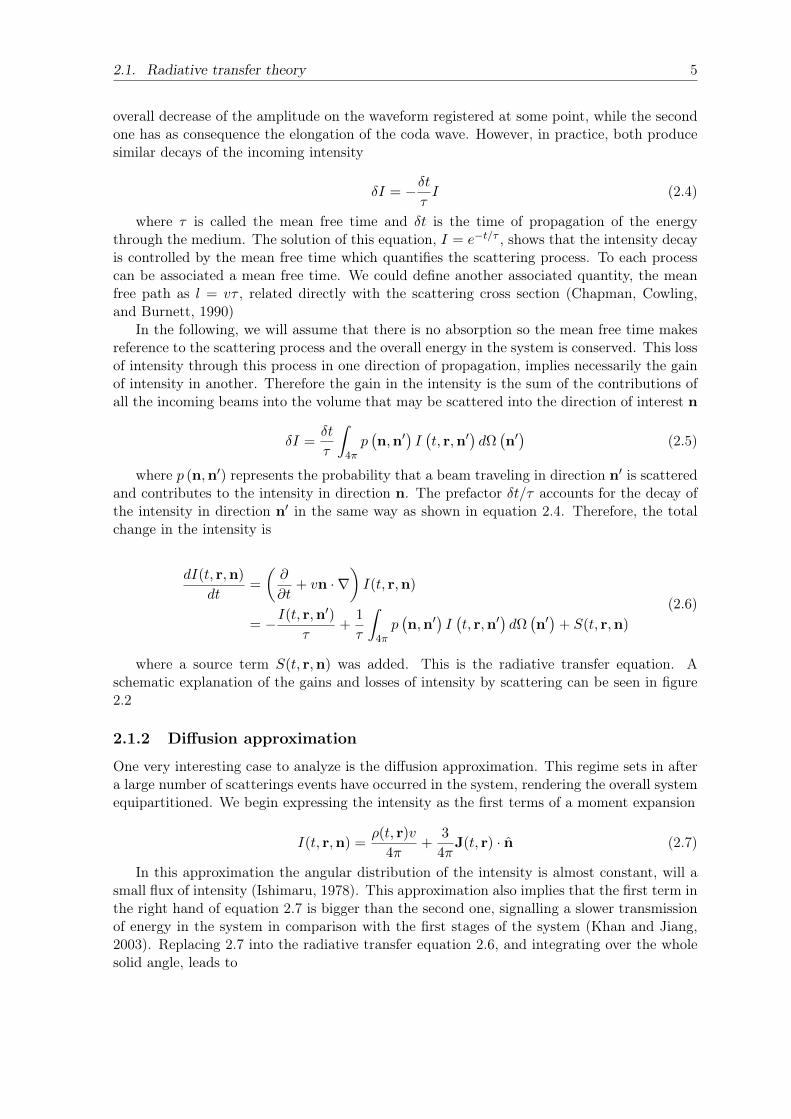
2.1. Radiative transfer theory 5
overall decrease of the amplitude on the waveform registered at some point, while the secondone has as consequence the elongation of the coda wave. However, in practice, both producesimilar decays of the incoming intensity
δI = −δtτI (2.4)
where τ is called the mean free time and δt is the time of propagation of the energythrough the medium. The solution of this equation, I = e−t/τ , shows that the intensity decayis controlled by the mean free time which quantifies the scattering process. To each processcan be associated a mean free time. We could define another associated quantity, the meanfree path as l = vτ , related directly with the scattering cross section (Chapman, Cowling,and Burnett, 1990)
In the following, we will assume that there is no absorption so the mean free time makesreference to the scattering process and the overall energy in the system is conserved. This lossof intensity through this process in one direction of propagation, implies necessarily the gainof intensity in another. Therefore the gain in the intensity is the sum of the contributions ofall the incoming beams into the volume that may be scattered into the direction of interest n
δI =δt
τ
∫4πp(n,n′
)I(t, r,n′
)dΩ(n′)
(2.5)
where p (n,n′) represents the probability that a beam traveling in direction n′ is scatteredand contributes to the intensity in direction n. The prefactor δt/τ accounts for the decay ofthe intensity in direction n′ in the same way as shown in equation 2.4. Therefore, the totalchange in the intensity is
dI(t, r,n)
dt=
(∂
∂t+ vn · ∇
)I(t, r,n)
= −I(t, r,n′)τ
+1
τ
∫4πp(n,n′
)I(t, r,n′
)dΩ(n′)
+ S(t, r,n)
(2.6)
where a source term S(t, r,n) was added. This is the radiative transfer equation. Aschematic explanation of the gains and losses of intensity by scattering can be seen in figure2.2
2.1.2 Diffusion approximation
One very interesting case to analyze is the diffusion approximation. This regime sets in aftera large number of scatterings events have occurred in the system, rendering the overall systemequipartitioned. We begin expressing the intensity as the first terms of a moment expansion
I(t, r,n) =ρ(t, r)v
4π+
3
4πJ(t, r) · n (2.7)
In this approximation the angular distribution of the intensity is almost constant, will asmall flux of intensity (Ishimaru, 1978). This approximation also implies that the first term inthe right hand of equation 2.7 is bigger than the second one, signalling a slower transmissionof energy in the system in comparison with the first stages of the system (Khan and Jiang,2003). Replacing 2.7 into the radiative transfer equation 2.6, and integrating over the wholesolid angle, leads to

6 Chapter 2. Concepts and methods
I(n)
I(n’)
I(n’)Lost I
Gained I
Gained I
Figure 2.2: Schematic view of the gains and losses of intensity by scattering. The black lines rep-resents the incoming specific intensity I(n), and the red and purple lines represent specific intensities
that end up contributing to I(n). In this particular case the total intensity increases.
v
3∇ρ(t, r) +
1
v
∂J(t, r)
∂t= −J(t, r)
l
(1− 1
4π
∫4πp(n · n′)n · n′ dΩ
(n′))
(2.8)
The last term in parenthesis accounts for the possible scattering anisotropy of the systembetween the incoming n and scattered n′ directions of the intensity. Notice, however, how thisterm depends in their relative directions only and not in the absolute direction of propagationof the intensity which indicates the isotropy of the medium. Since n ·n′ = cos θ where θ is theangle between the two directions, the right hand side term in the parenthesis in equation 2.8can be interpreted as the weighted average -〈cos θ〉- of the cosine of the scattering angle overthe whole solid angle. Assuming that ∂J/∂t = 0 we arrive to the first Fick’s law of diffusion(Bergman et al., 2011)
J(t, r) = −D∇ρ(t, r) (2.9)
where D is the diffusivity, that on this particular case is D = vl?/3 where
l? =l
1− 〈cos θ〉 (2.10)
is called the transport mean free path. This means that the velocity of the diffusion processis controlled by the scattering anisotropy, tending to be higher for bigger values of l?. In theparticular case where the scattering is isotropic l? = l and we get the lowest possible value ofD. When there is scattering anisotropy, the beam of energy tends to conserve the direction ofpropagation for a longer distance that the mean free path; in this sense, the transport meanfree path can be interpreted as the distance over which the energy lost all information aboutits original direction.

2.2. Equipartition of the energy 7
2.2 Equipartition of the energy
One common feature to all scattering systems is that they eventually reach to a diffusive statein which each normal mode is excited equally, independently of the initial conditions of thefield. The amount of energy is proportional to the number of modes that can be sustained inthe medium (Hill, 1986; Morse and Bolt, 1944), or in other words, to the density of states; forexample, in an elastic medium there can be two transversal modes of propagation (s-waves),and one longitudinal (p-wave). Then, the energy partition between the two types of waves is(Weaver, 1982)
R =EsEp
= 2c3αc3β
(2.11)
where cα and cβ are the velocities of P-waves and S-waves respectively. The density ofstates can also be calculated in another way: the Green’s function of a linear operator L canbe defined as
[z − L(r)]G(r, r′
)= δ
(r − r′
)(2.12)
where z is a complex variable, and L represents the wave equation operator. L has a setof eigenfunctions un and eigenvalues λn that per definition obey the following relation
L(r)un(r) = λnun(r) (2.13)
Each eigenfunction represents the a normal mode in the system. It can be shown that thespectral representation of the Green’s function is an analytic function except for the pointswhere z = λn, which means that it diverges at the resonant modes of the system (Economou,2006). This important property can be used to isolate and count the normal modes of thesystem with the Green’s function. As an example, the density of states ρ for the Helmholtzequation can be expressed as (Sheng and Tiggelen, 2007)
ρ(ω, r) = −dk2(ω)
dω
1
πImG
(ω, r = r′
)(2.14)
where ω represents the frequency, and k the wavenumber.The equipartition of the energy was observed by Shapiro et al. (2000) and later by Hennino
et al. (2001) who made a series of observations theoretical estimations of equipartition ratiosin different combinations of seismic waves. Margerin, Campillo, and Van Tiggelen (2000)studied numerically the equipartition time in inhomogeneous elastic media using Monte Carlosimulations that included mode conversions and polarization.
2.3 Coda wave interferometry
The seismic wavefronts propagating through the earth get distorted by the interaction withheterogeneities that scatter a fraction of their energy in different directions. This processproduces the characteristic coda wave segments after the main arrivals in the seismograms(Aki, 1969). Although complicated to analyze, the coda wave is not random and can beunderstood as the superposition of all the possible wave fronts that propagated through manydifferent paths when going from the source to the receiver (Sato and Fehler, 2012). This impliesthat a complex seismogram generated by a seismic event can be reproduced if, by some mean,we repeat the same seismic source at the same position; this has been observed with twoor more earthquakes that occur in the same location with very similar magnitudes (Geller
8 Chapter 2. Concepts and methods
and Mueller, 1980; Poupinet, Ellsworth, and Frechet, 1984; Beroza, Cole, and Ellsworth,1995). However, although very similar, the received waveforms at the surface are not exactlyequal: small variations are produced as a consequence of small changes of the propertiesof the medium that happen in the period of time between the two seismic events. This isthe main principle behind some studies that use these alike earthquakes, called doublets, totrack the changes in the velocity (Poupinet, Ellsworth, and Frechet, 1984; Ratdomopurbo andPoupinet, 1995) or in the attenuation (Beroza, Cole, and Ellsworth, 1995) of the crust. Wealso refer the reader to Sato (1988) for a review of temporal variations of attenuation detectedwith coda waves. Coda wave interferometry (CWI) is the use of the coda of a waveform todetect an locate all these changes in the medium.
CWI has been applied in experiments to monitor changes of ultrasound waves propagatingthrough granite, (Snieder et al., 2002; Grêt, Snieder, and Scales, 2006), in a volcano usingits natural mild repeating explosions(Grêt et al., 2005), in concrete induced by thermal vari-ations (Larose et al., 2006), in the crust as a consequence of earthquakes (Nishimura et al.,2000; Peng and Ben-Zion, 2006), and associated to structural changes preceding eruptions(Ratdomopurbo and Poupinet, 1995; Wegler et al., 2006).
From the assumption of superposition of the field, the travel-time perturbation 〈τ〉 pro-duced by a small perturbation of the propagation velocity between a source and a receiver,can be understood as the average of the travel time perturbations τP generated between allthe possible trajectories P (Pacheco and Snieder, 2005; Snieder, 2006)
δt = 〈τ〉 =
∑P IP τP∑P IP
(2.15)
where IP represents the energy intensity of the wave that has propagated along pathP . This result is very interesting as it establishes a relationship between the eventual phaseperturbations of the coda waves and the energies arriving to a certain point which are the mainphysical quantity of the radiative transfer theory that assumes that the phases cancel eachother at the receiver. This is fundamental in the conceptual development of the sensitivitykernels.
With coda wave interferometry it is possible to relate different type of perturbations tomeasurements made in the coda. These perturbations can be of different nature: velocityfluctuations, random displacements of punctual scatterers and perturbations in the positionof the source (Snieder et al., 2002; Snieder, 2006); here we focus on the first one. A typicalphase change in the waveform recorded at the surface, generated by a change in the velocityof a medium can be seen in figure 2.3. The difference between the waveforms obtained withand without the velocity change increases proportionally to the time that the wave has spenttraveling in the medium. In this case, the relationship between the velocity variation andthe phase delay at different lapse times is −δt/t = δv/v. The quantity −δt/t is called theapparent velocity variation, also denoted ε by some authors. The term apparent is addedbecause when the velocity is changed in only one part of the medium, there is still a changein the phases at the surface, but the quantity −δt/t is not necessarily equal to the velocitypertubation δv/v in the medium anymore.
2.3.1 MCSW method
In monitoring, a linear relation between the phase delay and the velocity change in the mediumis assumed; therefore, the apparent velocity variation is obtained as the slope of the phasedelay δt for different lapse times t. One of the main methods to estimate this slope is theMoving Cross Spectral Window (MCSW) also known as the doublets method, as it was firstproposed and used to analyze the phase differences between the coda generated by doublets

2.4. Seismic interferometry 9
Figure 2.3: Effect of the variation of velocity over a seismogram. The red line represents the obtainedwaveform after a decrease in the velocity of the whole medium in 1% with respect to an unperturbed
medium represented by the black line. Taken from Froment (2011)
earthquakes by Poupinet, Ellsworth, and Frechet (1984). The MCSW method is based on awell know property of the Fourier transform: let u(t) represent a signal and U(ω) = F [u(t)]its Fourier transform. Then the Fourier transform of temporal shifted version of this signalu(t± δt) is (Pinsky, 2008)
F [u(t± δt)] = U(ω)e±iωδt (2.16)
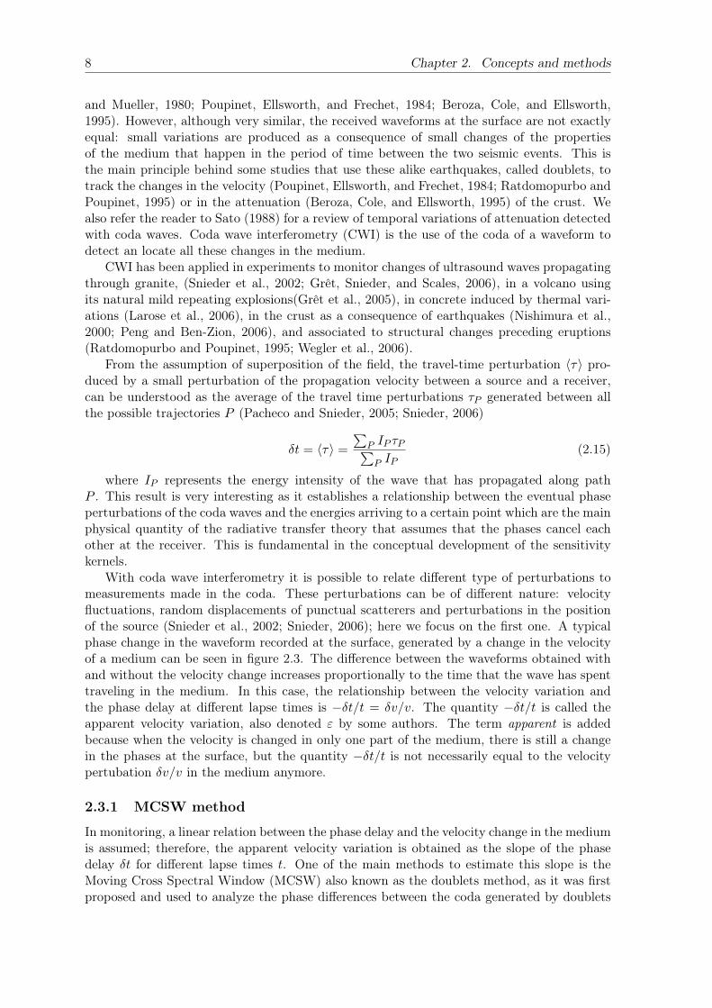
Notice how this temporal shift affects different frequencies at different degrees; a compar-ison between the Fourier transform of the original and the shifted signals would show a linearrelationship between their phase differences and the frequency. In this way, the δt can beestimated for a small section of the coda of the two signals. Since this delay is different fordifferent lapse times, this procedure is repeated over a window that is systematically movedalong the coda. This procedure is schematized in figure 2.4. In the end, a linear regression isperformed between the obtained values of δt and their respective lapse times to obtained theapparent velocity estimation.
2.4 Seismic interferometry
The link between recordings of correlations of noise and the properties of the medium can betraced back to early works done in helioseismology (Duvall et al., 1993; Giles et al., 1997).Later, a formal connection of these cross-correlations with the retrieval of the Green’s func-tion of the medium was established (Weaver and Lobkis, 2004; Lobkis and Weaver, 2001;Wapenaar, 2004). The Green’s function represents the response that one part of the system(in this case, the displacements on the surface) would have as a consequence of an impulsiveunit source in the medium. This relationship permits the use of tools of analysis in seismol-ogy that pass from monitoring to imaging, to regions where there is no presence of activesources. The reconstruction of the Green’s function using ambient seismic noise is calledSeismic Interferometry (SI).
Let u (t,x1) and u (t,x2) denote time dependent displacements recordings of noise seismicfield at two points over the surface. Then the noise cross correlation over a time interval [0, T ]can be written as
CT (τ,x1,x2) =1
T
∫ T
0u (t,x1)u (t+ τ,x2) dt (2.17)
10 Chapter 2. Concepts and methods
Figure 2.4: Moving Cross Spectral Method. Top: a reference signal (black), the signal registeredwith a velocity perturbation (red), and the window to be analyzed (zone in gray). Middle left: zoomof the differences between the coda segments highligthed section in gray in the top. Middle right:linear relation between the phase and the frequency as product of the time shift between. Bottom: δt
measured at different lapse times. Taken from Hadziioannou (2011)
2.4. Seismic interferometry 11
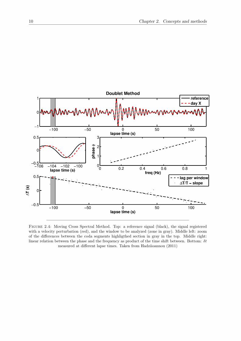
Figure 2.5: Cross correlation of recordings at two stations (triangles) from a seismic noise fieldgenerated by a random distribution of sources (circles). Taken from Garnier and Papanicolaou (2009)
where τ represents the time lag between the two signals. In a diffusive, equipartitionedfield it can be shown that (Snieder, 2004; Roux et al., 2005a)
∂
∂τCT (τ,x1,x2) = G (τ,x1,x2)−G (−τ,x1,x2) (2.18)
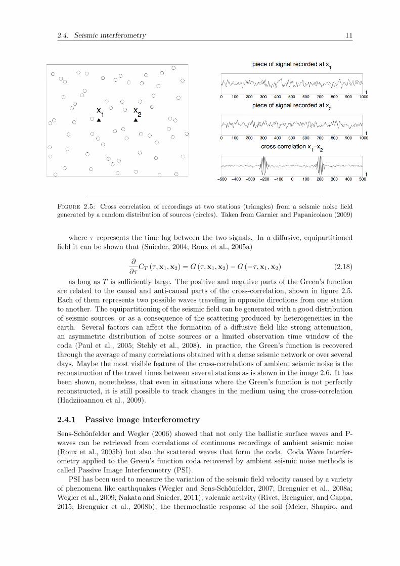
as long as T is sufficiently large. The positive and negative parts of the Green’s functionare related to the causal and anti-causal parts of the cross-correlation, shown in figure 2.5.Each of them represents two possible waves traveling in opposite directions from one stationto another. The equipartitioning of the seismic field can be generated with a good distributionof seismic sources, or as a consequence of the scattering produced by heterogeneities in theearth. Several factors can affect the formation of a diffusive field like strong attenuation,an asymmetric distribution of noise sources or a limited observation time window of thecoda (Paul et al., 2005; Stehly et al., 2008). in practice, the Green’s function is recoveredthrough the average of many correlations obtained with a dense seismic network or over severaldays. Maybe the most visible feature of the cross-correlations of ambient seismic noise is thereconstruction of the travel times between several stations as is shown in the image 2.6. It hasbeen shown, nonetheless, that even in situations where the Green’s function is not perfectlyreconstructed, it is still possible to track changes in the medium using the cross-correlation(Hadziioannou et al., 2009).
2.4.1 Passive image interferometry
Sens-Schönfelder and Wegler (2006) showed that not only the ballistic surface waves and P-waves can be retrieved from correlations of continuous recordings of ambient seismic noise(Roux et al., 2005b) but also the scattered waves that form the coda. Coda Wave Interfer-ometry applied to the Green’s function coda recovered by ambient seismic noise methods iscalled Passive Image Interferometry (PSI).
PSI has been used to measure the variation of the seismic field velocity caused by a varietyof phenomena like earthquakes (Wegler and Sens-Schönfelder, 2007; Brenguier et al., 2008a;Wegler et al., 2009; Nakata and Snieder, 2011), volcanic activity (Rivet, Brenguier, and Cappa,2015; Brenguier et al., 2008b), the thermoelastic response of the soil (Meier, Shapiro, and
12 Chapter 2. Concepts and methods
Figure 2.6: Cross correlations from stations around the globe. The late arrivals (after and before∼ ±5000s) correspond to surface waves that have traveled between the two stations making a turn
around the earth. Taken from Nakata, Gualtieri, and Fichtner (2019)
Brenguier, 2010), clay landslide (Mainsant et al., 2012), pressurized water injection (Hillerset al., 2015), internal erosion in earthen dams (Planès et al., 2016), the earth tides producedby the sun and the moon (Sens-Schönfelder and Eulenfeld, 2019), temperature variations dueto periodic heating of the lunar surface by the sun (Sens-Schönfelder and Larose, 2008), andvariations in the loading and pore pressure perturbations over and below the glacial cover(Mordret et al., 2016). Analysis of the ambient noise can also be used to predict earthquakeground motion (Prieto and Beroza, 2008) and study the seismic response of civil structures(Prieto et al., 2010; Nakata et al., 2013).
Many studies focus on the hydrological effects on the δv/v: Sens-Schönfelder and We-gler (2006) estimated the underground water level using a model developed by Akasaka andNakanishi (2000), to make a direct relation with the measured velocity variations in a vol-cano. Meier, Shapiro, and Brenguier (2010) analyze velocity variations within the Los Angelesbasin and conclude that the seasonal variations are strongly influenced by groundwater levelchanges and thermo-elastic strain variations. Tsai (2011) proposed periodic models to recre-ate displacements and velocity changes from thermo-elastic stresses or hydrological loadings.Wang et al. (2017) found a direct relation between velocity variations and several hydrologicaland meteorological processes across Japan, mainly based on the pore pressure generated bythe rainfall water through a diffusion process. Hillers, Campillo, and Ma (2014) also show thecorrelation between velocity changes and periodicity of precipitation events in Taiwan.
2.5 Sensitivity kernels
2.5.1 Observation and motivation
The phase fluctuations generated in the surface as a consequence of the presence of a bulkvelocity perturbation do not necessarily have a linear relationship with the lapse time; theirrelationship depends on the position and size of the perturbation. The behavior of the ap-parent velocity variation δt/t for two opposite cases is shown in figure 2.7. These resultsare obtained in a 2-D elastic medium with both the source and the receivers located at the

2.5. Sensitivity kernels 13
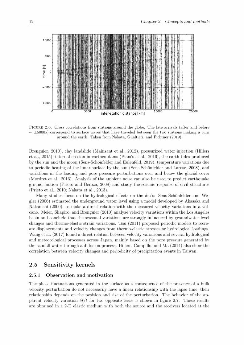
Figure 2.7: Apparent velocity variation for a perturbation made in a layer at 20m (left) and at1.5km (right) from the surface in an elastic 2-D heterogeneous medium. Taken from Obermann et al.
(2013a)
surface. Both are examples of the apparent velocity perturbations measured on the surfacewhen the velocity of a whole layer in a medium is slightly modified. At the left the δt/t mea-surements are obtained when the layer is located close to the surface, and at the right whenthe perturbation is deeper in the medium. In the first one, the apparent velocity variation atearly times is high as the perturbed layer is quickly sampled by most of the energy emittedby the source; however, it quickly decreases as the seismic field expands into deeper regions,making the perturbation relatively smaller in comparison with the total explored area. In thesecond case, the perturbation is only detected by the front of the propagating energy at thebeginning and is later sampled progressively more with the ongoing expansion of the wavefield. Notice that the magnitudes also change dramatically: in the latter case, δt is one orderof magnitude smaller than in the former case. This simple example shows that the differenceof behavior of the apparent velocity variation opens the possibility of estimating the shapeand location of the perturbation with the measurements made on the surface: this is the mainobjective of developing the travel-time sensitivity kernels.
The travel-time sensitivity kernel was first introduced by Pacheco and Snieder (2005) forthe diffusive regime, and by Pacheco and Snieder (2006) for the single scattering regime. Thesesensitivity kernels relate a travel-time perturbation measured between a source and a receiverwith all the possible velocity perturbations in the medium around them. For the first one,an analytical expression was obtained for the autocorrelation configuration (coincident sourceand receiver) for two and three dimensions and was compared against numerical simulationswhere a small perturbation is introduced. The travel-time sensitivity kernel for the singlescattering regime was calculated following the approach of Sato (1977) to obtain the energydensity of scattered waves assuming single isotropic. Later Planès et al. (2014) introducedthe decorrelation sensitivity kernel that related a perturbation in the medium that altersthe paths going from the source to the receiver, with the distortion that it generates to thewaveform at the receiver. Later Margerin et al. (2016) made an alternative derivation of thiskernel and extended the travel-time sensitivity kernel to include the direction of the energypropagation with the use of the specific intensity. In this work was proposed the idea that thedifference between the travel-time and the decorrelation sensitivities depended on whetherthe perturbation had an active or passive role over the generation of new propagation pathsbetween the source and the receiver. Applications like localizing perturbations in numerical
14 Chapter 2. Concepts and methods
simulations have been done using the sensitivity kernel. The decorrelation sensitivity kernelwas successfully used in locating millimetric holes drilled in a concrete sample (Larose et al.,2010). The sensitivity kernels can be expressed as convolutions of intensity which makesthe radiative transfer theory a natural tool for their estimation; Lesage, Reyes-Dávila, andArámbula-Mendoza (2014), for example, makes use of a solution of the transport equationsfor 2-D to locate changes produced by volcanic activity. On the other hand, Obermann et al.(2016) makes use of the 3-D radiative transfer solution proposed by Paasschens (1997) toestimate the body wave sensitivity kernel.
The coupling between body and surface waves has remained one challenging factor to thedevelopment of the sensitivity kernels in a 3-D halfspace that is the usual setting for mostseismic applications. Obermann et al. (2013a) and Obermann et al. (2016) approached thisproblem by expressing the sensitivity as a linear combination of two independent sensitivities,one for surface and another for body waves, with a controlling factor mediating between themthat changes with time, and that is estimated by comparisons with full wavefield numericalsimulations. These studies show the predominance of surface waves at early lapse times and ofbody waves at late lapse times. However, Wu et al. (2016) measured velocity variations fromthe phase of the Rayleigh waves obtained by seismic interferometry, and observed a progressivedecrease of the velocity drop produced by the 2004 Parkfield earthquake (Brenguier et al.,2008a) at lower frequencies. Since the surface waves penetration increases at lower frequencies,they conclude that the velocity variation is mostly constrained in the surface. Furthermore,they concluded that the observations can be explained only by the surface wave dispersionas body wave sensitivity would produce both velocities decreases and increases at differentpoints; this last affirmation was supported by travel-time sensitivity kernels that show that ina spherical geometry, direct shear waves may have alternating early or late arrivals dependingon the position on the surface of the receiver (Stein and Wysession, 2009; Zhao, Jordan,and Chapman, 2000). Similar findings were reported by Nakata and Snieder (2011) thatfound that the magnitude (MW ) 9.0 Tohoku-Oki earthquake produced a shear wave velocityreduction limited to the first 100m of the crust, despite being extended to an area 1200kmwide by comparing arrival times between stations located at the surface and in a borehole inranges of 100m to 337m depth. This, however, contradicts Wang et al. (2019) that through aninversion made with seismic and long-period tiltmeters data, found that the same earthquakeproduced changes that reach 40km depth in the crust.
2.5.2 Basic theory of traveltime sensitivity kernels
We begin with a concise derivation of the travel-time sensitivity kernel for a diffusive mediumfollowing its intensity interpretation (Pacheco and Snieder, 2005), and later make a connectionwith the more general version based on the specific intensities (Margerin et al., 2016). Letus imagine a normalized intensity impulse generated at a source, that propagates through amedium. The intensity at lapse time t at a point r is then described by P (r, t). If there is nomechanism of intrinsic attenuation acting on the system, the total energy at time t
W (V, t) =
∫VP (r, t)dV (r) (2.19)
is always equal to 1, that is, the total energy emitted by the source. The normalizationof the intensity allows us to make two additional interpretations of this quantity: P (r, t)represents the probability that a particle, following a random walk, arrives or passes by theposition r at time t (Roepstorff, 2012). P (r, t) can also be understood as the Green’s functionof the diffusion equation at position r at time t. The probability that a particle that was

2.5. Sensitivity kernels 15
Figure 2.8: Random walk of a going from the source, passing through a small volume dV andarriving to the receiver. Taken from Pacheco and Snieder (2005)
emitted at the source at s arrives to the receiver at r at time t, can be written in terms of thetransit of the phonon through a volume dV located at r′ at time t′ (illustrated in figure 2.8).
P(r, s, t+ t′
)=
∫VP(r, r′, t− t′
)P(r′, s, t′
)dV(r′)
(2.20)
This is the Chapman-Kolmogorov equation (Ross, 2014; Papoulis and Pillai, 2002; Roep-storff, 2012) which states that the probability of going from the source to the receiver canbe written by using the intermediate point r′ at a time t′, as long as all of them are takeninto account. Each of the terms involved in the last equation are transition probabilities; forexample
P(r′, s, t′
)= P
(r′, t′|s, t = 0
)(2.21)
is the probability that particle transits the position r′ at time t′, under the condition thatit was emitted from the source at position s and at time t = 0. An integration over all thepossible travel-times of these equations leads to
t =
∫V
[∫ t
0
P (r, r′, t− t′)P (r′, s, t′)P (r, s, t)
dt′]dV (r′) (2.22)
The term inside the square parenthesis is the sensitivity kernel K. One of the mostremarkable features of the kernel is that it expresses the travel time as a spatial distributionover the volume around the source and the receiver. An observer that could follow all thephonons going from the source to the receiver, could measure the sensitivity as the averagetime spent inside each volume of the medium (Margerin et al., 2016); therefore, the sensitivitykernels show which parts of the medium are preferred by the particles when going from thesource to the receiver. As such, the regions around the source, the receiver, and betweenthem, are zones that we expect to have high sensitivity as they are probably very frequentedby the phonons that travel between the two. A simple schematic explanation of the travel-time sensitivity can be seen in figure 2.9. From equation 2.22 we can estimate the travel-timelags at the surface generated by a velocity perturbation in the medium
〈δt〉t
= −∫VK(r′, t) δvv
(r′)dV(r′)
(2.23)

16 Chapter 2. Concepts and methods
(a) A single particle travels between the source andthe receiver
(b) Its travel-time can be distributed in small partsthrough the medium
(c) A second particle makes a different path betweenthe source and the receiver
(d) Their travel-times distributions can be added be-tween them
(e) Once normalized we have an image of the sensibil-ity kernel. The sum of all the times in this distribution
is equal to the travel time
(f) If done with many particles, some areas will havehigher sensitivity (red) than others (yellow)
Figure 2.9: Explanation of the travel-time sensitivity calculation between a source (at left) and areceiver (at right) with two phonons.
2.5. Sensitivity kernels 17
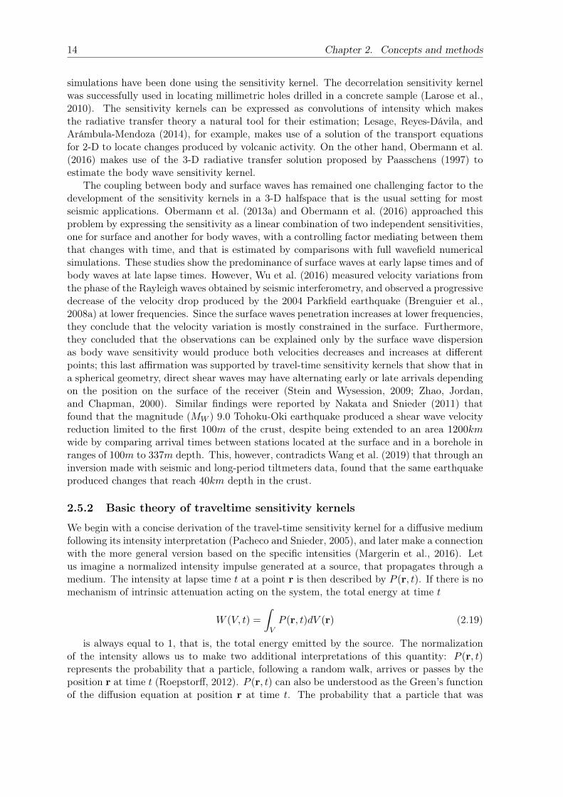
Figure 2.10: Travel-time sensitivity kernel for isotropic (left) and strongly anisotropic scattering(right). The kernels are symmetric between a source and the receiver. The distances have been
normalized by the mean free path. Taken from Margerin et al. (2016)
where 〈· · · 〉 represents the average travel time change generated by all the volume elements.This shows that in principle, the location of the perturbation can be done inverting from theinformation of the phase delays at the surface, and the kernels. However, the estimation ofthe kernel is usually a complicated task and in most cases, the solutions are estimated throughnumerical methods.
A second important interpretation can be made from equation 2.22: the sensitivity kernelis a convolution between the intensity perceived at r′ by the pulse generated at the source,and the intensity perceived at the receiver by the pulse generated at r′. Many of the studiesdone with the sensitivity kernels were based on this kernel for diffusive waves, and the kernelfor a single scattering model (Pacheco and Snieder, 2006). Margerin et al. (2016) unified andextended these cases with the use of the specific intensity, allowing them to track the seismicfield within its early period, which is strongly marked by the directionality of the energyradiation. With this new approach, the sensitivity kernel can be written as
K(r′, t; r, r0
)= S
∫ t
0
∫S
P (r, r′, t− t′,−n′)P (r′, s, t′,n′) dt′dn′
P (r, s, t)(2.24)
where n represents the direction of propagation of the phonons in the volume dV , andS represents its area. This kernel introduces the direction of the particles in the Chapman-Kolmogorov equation in addition to their positions. This also allowed the theory to includeanisotropic scattering. The travel-time sensitivity kernel obtained for isotropic and stronganisotropic scattering can be seen in image 2.10.

19
Chapter 3
Separation of phenomena from δv/vmeasurements
Andres Barajas, Piero Poli, Nicola D’Agostino, Ludovic Margerin, Michel CampilloArticle in preparation
There is a wide variety of phenomena that can affect the properties of the crust of theEarth. For this reason, it is usual that measurements of the apparent velocity variation ob-tained from recordings from ambient seismic noise, present variations that are the sum of thesimultaneous action of these phenomena. Identifying to what degree an apparent velocityvariation in the surface is caused by a certain physical process is a challenging work that usu-ally requires the cross-examination and comparison with independent sources of informationbeyond the velocity itself. In this chapter, we present one effort in this direction in the Pollinoregion, Italy. This area was chosen because most of its seismic activity is limited to a relativelysmall period within the time frame of study, and because some exploratory measurements ofthe velocity variation in the zone showed interesting patterns. The advantage of having aperiod free of seismic activity is the possibility of having a control set against which we cancompare the velocity changes when there is seismic activity. Another very important aspect ofthis region is the presence of aquifers as it is well known that the water content in the crust isone of the main factors behind the velocity variation of the seismic waves. Furthermore, thereis a well-preserved record of the rainfall of the zone and a good distribution of GPS stations inthe area that make this region an ideal subject of study. In this chapter following the standardnotation, the term δv/v is referred to as the measured or apparent velocity variation; behindthis is the usual assumption of a linear relationship between the actual velocity perturbationat depth and the apparent velocity variation at the surface. However, in later parts of thisthesis, the distinction between both will be necessary and therefore δv/v will be reserved forthe actual variation at depth, and −δt/t for the apparent velocity changes measured at thesurface.
3.1 Abstract
Analysis of the ambient seismic noise has proven to be a powerful tool to infer the structureor dynamic of the crust through the measure of the variation of the seismic field velocity.However, given the high sensitivity of this method, it’s common to register velocity variationsproduced by many different factors like seismic events or changes in the crust due to atmo-spheric phenomena. In this study, we aim to disentangle these processes from a ten-year-longrecording of seismic noise made with a single station in the region of Pollino, in the south ofItaly. This region is characterized by the presence of aquifers and by a relatively short periodof high seismic activity which includes slow slip events, and a M5.0 earthquake that occurredthe 25 October 2012.
20 Chapter 3. Separation of phenomena from δv/v measurements
We apply two models that estimate the water level inside the aquifer assuming it is con-tinuously recharged from the rainfall of the region. We find that both models make a goodprediction of the measured δv/v which means that the velocity variation is driven by changesin the pore pressure inside the aquifer: an increase of the water level produces a decrease inthe seismic velocity in the zone. Our interpretation of the dynamic inside the aquifer is fur-ther confirmed by geodetic measurements which show that in a direction parallel to the strikeangle of the fault rupture, the displacement of the zone follows the same patterns observed inthe models and in the velocity variation. This could be understood as a poroelastic behaviorin which the aquifer expands and contracts due to the pressure generated by the water on itsinterior, which also causes the velocity changes.
Going one step further, we analyze the nature of the small discrepancies between themeasured and modeled velocity variations. We find that these are well correlated with therainfall and with the vertical geodetic measures, which points to an instantaneous elasticresponse of the zone to the loading generated by the rain. The comparison between thesevariables allows us to make a clear identification of the period of seismic activity in the zone,represented by the characteristic drop in the seismic velocity in the period from the beginningof 2012 to mid-2013.
3.2 Introduction
The analysis of the ambient seismic noise (Campillo and Paul, 2003; Shapiro and Campillo,2004; Campillo, 2006) has permitted estimate changes in the velocity in the crust related toa variety of phenomena, like earthquakes (Brenguier et al., 2008a), volcanic activity (Rivet,Brenguier, and Cappa, 2015; Brenguier et al., 2008b) and the thermoelastic response of the soil(Meier, Shapiro, and Brenguier, 2010), among others. Many studies focus on the hydrologicaleffects on the δv/v. Sens-Schönfelder and Wegler (2006) estimated the underground waterlevel using a model developed by Akasaka and Nakanishi (2000), to make a direct relation withthe measured velocity variations in a volcano. (Meier, Shapiro, and Brenguier, 2010) analyzevelocity variations within the Los Angeles basin and conclude that the seasonal variations arestrongly influenced by groundwater level changes and thermo-elastic strain variations. Tsai(2011) propose periodic models to recreate displacements and velocity changes from thermo-elastic stresses or hydrological loadings. Wang et al. (2017) found a direct relation betweenvelocity variations and several hydrological and meteorological processes across Japan, mainlybased on the pore pressure generated by the rainfall water through a diffusion process. Hillers,Campillo, and Ma (2014) shows the correlation between velocity changes and periodicity ofprecipitation events in Taiwan.
Hydrological deformation processes have also been studied through geodetic data (Bawdenet al., 2001; Watson, Bock, and Sandwell, 2002; Borsa, Agnew, and Cayan, 2014; Chanardet al., 2014). In general, the effects of rainfall can be seen in two possible ways: as an elasticresponse where the water exerts a loading pressure that subsides the surface (Amos et al.,2014; Argus, Fu, and Landerer, 2014; Nof et al., 2012), or as a poroelastic response thatgenerates a rise of the surface as a consequence of the recharge of the porous inner structureof the soil (Galloway and Burbey, 2011; King et al., 2007).
From the aforementioned studies emerge that thermal and hydrologic effects on δv/v aresignificant, and can thus mask velocity changes induced by tectonic processes. It is thusfundamental to quantify the environmental effect to resolve the tectonic induced velocityvariations for fault physics studies. Examples of this approach are the study of Hillers et al.,2019, where the seasonal variations were filtered out, to highlight deformation patterns oftectonic origin around the San Jacinto fault, or the work of Poli et al., 2020 where tectonic
3.3. Data processing description 21
and hydrological processes are separated from a single station analysis of the δ/v. In thisstudy we pursue this same objective: we disentangle the influence of the water content insidethe crust from the tectonic related events, in a δv/v time series obtained from ambient seismicnoise recorded in a single station in the region of Calabria, Italy (Figure 3.1).
One of the main characteristics of this zone is the presence of karst aquifers which islikely the driving factor behind geodetic of seismic velocity measurements (Poli et al., 2020;D’Agostino et al., 2018). Furthermore, this area was relatively inactive seismically until thebeginning of 2012, when began a seismic swarm that lasted until the middle of 2013, a periodthat included several earthquakes including a M5.0 event on the 25 October 2012 (Passarelliet al., 2015). It has been estimated that 75 percent of 6000 events detected during theswarms are not aftershocks, which means that there may be a transient forcing acting as thedriving mechanism behind the swarm. The physical nature of this transient forcing can befluid filtration, pore pressure diffusion, or aseismic slow slip (Parotidis, Rothert, and Shapiro,2003; Peng and Gomberg, 2010). This last scenario can also be associated with fluid-relatedphenomena reducing the normal stress in the fault. It has also been suggested that a bigpart of the crustal deformation in the zone is accommodated through transient slow slip event(Cheloni et al., 2017).
In this work, we apply two different models that calculate the water level inside the aquiferbased on the information of the rainfall and compare the obtained behavior with the seismicnoise-based velocity variations. We make an independent verification of the obtained resultsthrough horizontal geodetic measures of the zone. We also analyze at a deeper level thevelocity variation removing from it, the modeled behavior controlled by the water level insidethe aquifer. This allows us to identify a weaker pattern controlled mainly by the immediateelastic response of the zone to the rainfall which is also the main driving factor behind thevariations of the vertical geodetic measurements. Finally, this procedure reveals a velocitydrop most probably related to the stress release of the zone through seismic activity.
3.3 Data processing description
An overall layout of the data stations can be seen in figure 3.1. The seismic ambient noiseis recorded at the station MMNO in Pollino area (Italy) (INGV Seismological Data Centre,2006). The three components’ continuous signals were band-passed between 0.5Hz and 1Hz.For each day, the whole signal is divided into overlapping windows of half an hour (50% over-lap). Later, we calculated the cross-correlation between the 30-minutes windows for all thepossible combinations of the three available channels; this means that for each 30 minutessegment, we obtain 6 cross-correlations. In the practice, we calculate them simultaneously us-ing the Covet package (Seydoux, Rosny, and Shapiro, 2017). The half-hour cross-correlationsare average between them for each day, resulting in 6 cross-correlations per day. Two aver-aging processes for each combination is performed: the first one consists of making a movingaverage with the correlations of 30 days around each day to stabilize the obtained signal andreduce possible transient noise sources. The second consists of obtaining six global referencecross-correlations averaging between all the available days. A variation of the velocity canbe estimated if we consider that a perturbation in the medium will generate a change in theshape of the cross-correlation with respect to the global average, in the same way, that a pulseemitted in the position of the seismic station would be registered differently if the velocity ofthe medium change. We calculated this possible change in the frequency domain (Poupinet,Ellsworth, and Frechet, 1984) using the segment of the coda of the cross-correlations between10s and 50s. All the 6 velocity variations time series are averaged daily and finally, a movingaverage of 30 days is applied over the resulting δv/v series.
22 Chapter 3. Separation of phenomena from δv/v measurements
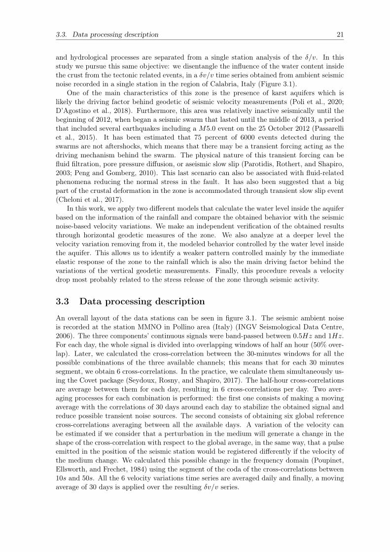
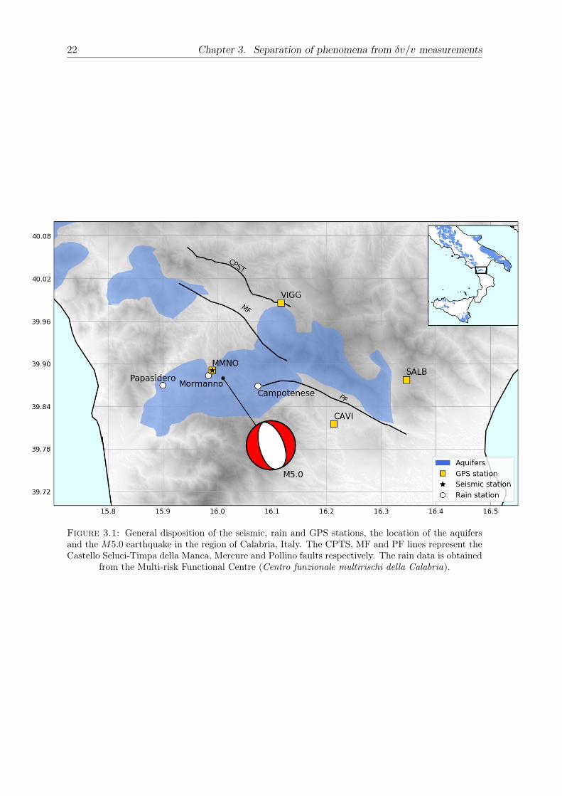
Figure 3.1: General disposition of the seismic, rain and GPS stations, the location of the aquifersand the M5.0 earthquake in the region of Calabria, Italy. The CPTS, MF and PF lines represent theCastello Seluci-Timpa della Manca, Mercure and Pollino faults respectively. The rain data is obtained
from the Multi-risk Functional Centre (Centro funzionale multirischi della Calabria).

3.4. Procedure and results 23
0.000
0.025
0.050
0.075
0.100
0.125
0.150
0.175
0.200
Dai
lyra
infa
ll(
mm
)
0
50
100
Sei
smic
Mom
ent
(a)
(b)−0.25
−0.20
−0.15
−0.10
−0.05
0.00
0.05
0.10
0.15
Vel
oci
tyva
riat
ion
(%)
2010 2011 2012 2013 2014 2015 2016 2017 2018 20190
200
400
Slip
-rat
e(mm/yr)
Slip-rate
Figure 3.2: a) Seismic measurements of δv/v and daily rainfall in the region. b) Daily accumulatedseismic moment in the region and reported slip-rate by Cheloni et al., 2017. The dashed line marks
the date of the M5.0 seismic event.
The GPS displacements were obtained from the Rete Integrata Nazionale GPS network(INGV Seismological Data Centre, 2006). This data was processed using the Jet PropulsionLaboratory (JPL) GIPSY-OASIS II software.
The rain data was collected in the 3 closest available stations shown in 3.1. Not all threestations have available data in all the studied period, so the average process is done each dayusing only the available information. The result of this process gives us the estimation of theregional daily rainfall show in figure 3.2a.
3.4 Procedure and results
3.4.1 Measured and modeled velocity variations
The noise-based velocity variations plotted in figure 3.2a reveal several patterns. We recognizea periodic ( 1 year) oscillation that is likely to be controlled by the amount of water in thecrust. Indeed, the daily rain observed on the region (fig. 3.2a) increase during the winter, withan associated velocity reduction (Sens-Schönfelder and Wegler, 2006). Beyond the periodicsignal, a long term trend of increasing velocity is observed for the full period (fig. 3.2a).
To separate hydrologic signal from the possible presence of tectonic stress change effectsin the seismic δv/v series, we model the induced velocity variations generated by the amountof water in the crust. For this, we developed and applied two different models allowing theestimation of accumulated water inside the aquifer as a function of time.

24 Chapter 3. Separation of phenomena from δv/v measurements
The aquifer is recharged with the rainfall through a fast process thanks to the characteristicpermeable material of the karst. We assume that this happens at a higher velocity than in anormal diffusion process: rainfall is added each day directly to the water level of the aquifer.The discharge process can be described by two different models, both of them related to thestored water inside the aquifer. The first one, the linear reservoir (Fiorillo, 2011), assumesthat the aquifer loses water through a flux with its surroundings, at a discharge rate dQ/dt(being Q the stored volume of water) that is proportional to the difference of concentrationbetween the interior and the exterior of the karst ∆φ, and the contact area between the twoAL
dQ
dt= UAL∆φ+R (3.1)
where R is any external source supplying the aquifer. In the last equation U plays the roleof a conductance over the surface, that is, the proportionality constant between the flux ofwater leaving the aquifer (per unit of area) and the concentration difference; in fact, U is theequivalent of the heat transfer coefficient in the heat transfer Newton’s law of cooling. Fromthis point of view, this is parallel to obtaining Newton’s law of cooling from the heat equationthat is described also as a diffusive process. The total quantity of water inside the aquifercan be written in terms of its density and the volume it occupies. The water in the aquiferaccumulates at its bottom, and therefore, this volume can be written in terms of the areaof the bottom AB and the height of the column of water h. On the other hand, we assumethat the area that transmits water is just the lateral one (no difference-of-concentration fluxat the top or at the bottom). Then, the contact area can be written approximately as themultiplication of a perimeter and the height of the column of water AL = P ∗ h. Introducingthese changes turn the discharge equation into
d (ABh)
dt= UPh∆φ+R (3.2)
that means that the rate at which the aquifer lose water is proportional to the water levelitself
dh(t)
dt= −kh(t) + r (3.3)
where h is the water level inside the aquifer, r is the source term written in terms of thechange it generates in the water level inside the aquifer and k = UP∆φ/AB that depends onthe geometry of the aquifer and the conductance of the medium.
The second model, the Torricelli reservoir (Fiorillo, 2011), assumes that the aquifer worksas a container that loses water through a spring at its bottom. The velocity at which thewater leaves the aquifer is proportional to the square root of the height of the contained water,as stated by Torricelli’s law
v =√
2gh (3.4)
where g represents the gravity. In this case, the discharge can be written in terms of thisvelocity, and the area through the water is escaping (As)
dQ
dt= Asv +R = As
√2gh+R (3.5)
If we write again the volume of water inside the aquifer as ABh, the change on the waterlevel will follow the same mathematical structure ,

3.4. Procedure and results 25
dh(t)
dt= −k′
√h(t) + r (3.6)
where k′ = As√
2g/AB, and r represents the source supplying the aquifer in terms of thewater level. The constants in both of these equations are related to the physical characteristicsof the aquifer, and modifying them changes the strength and the delay of the discharge for agiven water quantity inside the aquifer.
Therefore, the water level at each day will be the level of the day before, plus the levelgained by the rainfall on that day r, minus the losses that are calculated according to themodel:
hi+1 = hi − kf(hi) + ri+1 (3.7)
Here f(hi) represents the particular functional dependence of the model in the water level,defined by equation 3.3 or 3.6. At this point it’s important to remark the units of the waterlevel as obtained by the models: they are equal to the units of the rainfall, which is measuredas mm of water recollected per square meter. This means that only if we have an aquifer ofexactly 1m2, recollecting the totality of the indicated rainfall (that is most probably not thecase), we will have the water levels predicted by the models. Furthermore, if the area thatcollects the water (the area of the aquifer) is different from the area that supplies the rainfall,the proportion between both units will not be 1-to-1. This implies that both models allow usto predict relative changes in the water level, but not its absolute value. However, this is nota problem as will be clear below.
If the water level controls the velocity variation, the resulting series for h should show thesame behavior as the δv/v, or in other words, there would be a linear relationship betweenthem. We find the value of the constant k in each model that optimizes the linear relationbetween them with the following grid search:
• A value of k is chosen, and using the rain data as the input, the water level time seriesis calculated following the recursive formula 3.7
• The water level is shifted towards the zero removing its time average (represented by〈·〉):
h(t)→ h(t)− 〈h(t)〉 (3.8)
• The proportionality constant between (δv/v)(t) and the water level time series is calcu-lated as the ratio between the covariance and the variance: a = cov ((δv/v)(t), h(t)) /(var(h(t))
• The shift or intercept between the two series is estimated as the average of the seismicvelocity variation: b = 〈(δv/v)(t)〉
• A synthetic velocity variation δv/vsyn is obtained from the water level model using bothconstants a and b:
δv
v syn(t) =
⟨δv
v(t)
⟩+
(cov
(δvv (t), h(t)
)var(h(t))
)· h(t) (3.9)
• For a given constant k, the fit to the data of the model to describe the seismic velocityvariation is measured as
σ2(k) =1
n
n∑i=1
(δv
v(i)− δv
v syn(i, k)
)2
(3.10)

26 Chapter 3. Separation of phenomena from δv/v measurements
2010 2011 2012 2013 2014 2015 2016 2017 2018 2019−0.2
−0.1
0.0
0.1
Diff
eren
ce(%
) (b)
Residual δv/v
Slip-rate
0
500
1000
Slip
-rat
e(mm/yr)
−0.15
−0.10
−0.05
0.00
0.05
0.10
0.15
Vel
oci
tyva
riat
ion
(%)
(a)
(δv/v): Seismic measurements
(δv/v)syn: Water level model
Figure 3.3: Seismic noise measurements and water level model. a) Seismic and synthetic δv/vobtained from the water level model. b) difference between the model and the measured δv/v smoothedwith a 30 days window and reported slip-rate by Cheloni et al., 2017. The shaded zone highlightsthe systematic excess of velocity reduction between the seismic δv/v and the rain-based model. The
dashed line marks the date of the M5.0 seismic event
• The process is repeated for a whole set of values of k and the one with the lowest σ2 ischosen.
Both the models produce almost indistinguishable results because a daily input will high-light in the long term only a linear dependence with the input itself. The misfit of each modeland a comparison between them can be seen in the supplementary material. The predictedvelocity variation obtained with the linear reservoir model for the best fitting constant canbe seen in figure 3.3a; this will be the model used in the rest of the paper. In both cases thecovariance between the seismic measurements and the water level model is negative, whichmeans that they are anti-correlated: the increase of the water content in the aquifer decreasesthe seismic velocity in the medium. This happens because the presence of water increases thepore pressure, which in turn, reduces the overall effective pressure in the zone and therefore,reduces the seismic velocity. We can see that the models reproduce accurately the seismic-based series, not only on its seasonal patterns but also in the overall multi-year trend, whichmeans that the water content in the aquifer is effectively the main driving factor behind theregistered velocity variations. The positive trend observed between 2014-2019 is a regionalmulti-annual hydrological trend observed also in the spring discharge and in the modulationof seismicity along the Irpinia Fault (D’Agostino et al., 2018).
The difference between measured velocity changes and the modeled velocity changes canbe seen in figure 3.3b. It can be seen that there is a periodic misfit between them which

3.4. Procedure and results 27
means that a small part of the seismic velocity variation is not predicted by our models. Thiscould be due to a defect of the model or to the presence of a second phenomenon actingin parallel with the water accumulation. Furthermore, the most remarkable feature of thisdifference is a systematic excess of velocity reduction, that begins at the beginning of 2012when there is high seismic activity, and that lasts approximately until the end of 2014; thevelocity changes measured in the seismic field are not completely accounted by the waterlevel model, that is, by the accumulated water able to increase the hydraulic head and theaquifer pore pressure. Although the 1-month moving average applied over the time seriesmakes it difficult to talk about specific dates, this systematic difference is probably generatedby tectonic stress release as it happens simultaneously with the seismic activity. Furthermore,through 2013 this difference seems to increase and seems to have its maximum peak aroundthe same time of the last pulse of the reported slow slip in the zone. It was found that thislate slip happened simultaneously with an enlargement of the crustal area affected by theseismicity (Cheloni et al., 2017). However, the systematic difference with our model extendsbeyond the slow slip event for several months. This extended behavior could be related tothe stress change produced by the earthquake and its posterior recovery phase that could lastseveral months (Brenguier et al., 2008a). It could also be possible that the earthquake orthe slow slip changed the internal structures of the aquifer which will produce a migrationof water that would change temporarily the water level. Whatever may be the cause, thechanges in the velocity are completely recovered by the end of 2013.
3.4.2 Analysis of geodetic data
Geodetic measurements are useful to measure displacements related to earthquakes and toslow slip events, and also to analyze hydrological processes inside aquifers (Cheloni et al.,2017; D’Agostino et al., 2018; Silverii et al., 2016). We turn to analyze GPS traces as anindependent way to assess the modeled variation of the velocity and its possible mechanisms.For this, we use GPS traces obtained in four stations of the zone which are shown in figure3.1.
We begin analyzing the relative displacement between the two closest stations to theearthquake, VIGG and MMNO, smoothed with the same 1-month window as was done withthe velocity variation. Both relative horizontal components can be seen in figure 3.4a. Tosimplify the visualization of the GPS traces, all of them have been shifted vertically towardsthe zero without modifying their behavior or their relative values. This doesn’t affect ouranalysis as we are interested in the patterns described by the traces and not in their absolutevalues. The relative displacement shows seasonal patterns in all the directions and a clearchange of baseline due to the M5.0 event.
Perhaps the most interesting feature of the traces in figure 3.4a is the behavior of the NScomponent from 2014 until the end of the series, as it shows a similar pattern to the oneobserved in the δv/v: a yearly seasonal variation over a multiyear increasing behavior, withapproximately the same shape. However, this behavior is not present in the EW direction.There are a couple of reasons why this behavior can not be seen in both components. Oneof these is a possible anisotropic response of the aquifer to hydrostatic pressure in the hori-zontal direction (Silverii et al., 2016). Commonly, a porous medium like an aquifer presentsfractures than can open and close temporarily with the pressure generated by the water inthem (Amoruso et al., 2014; Daniele, Braitenberg, and Nagy, 2012). If these fractures happenpredominately in a specific direction, the macroscopic expansion-contraction dynamics will bemore (or only) visible in such direction, which constitutes an anisotropic response. Anotherpossible reason could be simply the relative position of the GPS station to the aquifer: forexample, if we had a GPS station at the north of a perfectly circular aquifer, we would expect

28 Chapter 3. Separation of phenomena from δv/v measurements
−15
−10
−5
0
5
GP
Sdi
spla
cem
ent
(mm
)
a)
EW
NS
−15
−10
−5
0
5
GP
Sdi
spla
cem
ent
(mm
)
b)
N126W
N36W
2010 2011 2012 2013 2014 2015 2016 2017 2018 2019
−0.15
−0.10
−0.05
0.00
0.05
0.10
0.15
Vel
oci
tyva
riat
ion
(%)
c)
(δv/v): Seismic measurements
(δv/v)syn: Water level model
(δv/v)syn: GPS N36W
Axis orientation
Figure 3.4: Modeled velocity variations and GPS relative displacements. a) Relative horizontalGPS displacements between stations MMNO and VIGG. b) GPS horizontal relative displacementsrotated by an angle of 36 in clockwise direction. c) Velocity variations measured through seismicnoise analysis, predicted from the water level model, and fitted with the rotated N36W horizontal
displacement. The dashed line marks the date of the M5.0 seismic event.

3.4. Procedure and results 29
2010 2011 2012 2013 2014 2015 2016 2017 2018 2019
−1.0
−0.8
−0.6
−0.4
−0.2
0.0
0.2
Vel
oci
tyva
riat
ion
(%)
δv/v
Seismic mesurements
Water level model
VIGG-MMNO N36W
VIGG-CAVI NS
VIGG-SALB N11W
MMNO-SALB N34W
MMNO-CAVI N36W
SALB-CAVI N29W
Figure 3.5: Comparison between the measured velocity variation (black) and all the syntheticvelocity variations obtained with the water level model (blue line) and with rotations of the GPSrelative displacements for all the possible combinations between the 4 stations. A shift of 0.15% wasintroduced between them for visualization purposes. The angle of the rotation that maximizes the fitfor each couple is indicated in the label of the line, with exception of VIGG-CAVI where no rotation
was needed. The dashed line marks the date of the M5.0 seismic event.
30 Chapter 3. Separation of phenomena from δv/v measurements
to see the expansion-contraction registered only in the NS component and not in the EWcomponent, even in an isotropic fracture system.
Likely, the main expansion-contraction direction is not exactly NS. With this in mind, weperform a rotation of the horizontal GPS traces to find the angle that maximizes the presumedlinear relation between the GPS displacement, and the modeled water level inside the aquifer.This is done through a similar grid search like the one implemented before, between onerotated component of the GPS and the measured seismic δv/v.
The reason why this angle minimizes the fit can be easily seen in figure 3.4c: the tracein the direction N39.3W shows the same behavior of the modeled velocity variations for alltimes, even in the period in which the earthquake and the slow slip happened. There may betwo reasons why this trace reproduces so well the water level in the aquifer: the fist one, thedirection of this rotated GPS is the only direction in which the fault rupture of the earthquakeis not visible, that is, the direction of the strike angle of the earthquake. This is importantas any other direction will show a discontinuity in the horizontal expansion of the aquifer.On the other hand, it’s possible that the localization of the GPS station, NW of the aquifer,helps to accentuate the expansion-contraction process in that specific direction.
Beyond the mechanism that accentuates one direction in particular, is clear that thebehavior of the displacements is related to the variations seen in both the velocity changes andin the water model, which is coherent with an expansion-contraction dynamics in the aquifer(Cheng, 2000). As the aquifer stretches between the four GPS stations, this process shouldbe visible by different combinations of stations and not only between VIGG and MMNO: ineffect, calculating the relative displacement between all the other couples, and finding the bestrotation for each case produce a similar pattern, as can be seen in the figure 3.5. Althoughdifferent GPS combinations are better fitted around different angles, all the combinationsthat involve the station MMNO (the closest to the seismic event) are maximized around 36degrees, possibly as a consequence of finding the projection that doesn’t show the effect of theearthquake itself. Moreover, it can be seen that different couples produce different levels ofintensity between the seismic event and the water-driven pattern, which signals a possible newway to analyze the complexity of the system, and particularly, the directions of volumetricexpansion of the zone.
3.5 Loading effect of the rainfall
A deeper inspection of the seismic velocity variations can be made if we analyze the part ofit that is not controlled by the water level in the aquifer. This can be done by subtractingone from another as is shown in figure 3.6a. This is the same difference shown in figure3.3 but processed with a longer smoothing window of 180 days to stabilize the fluctuationsand highlight seasonal patterns. The longer smoothing window and the fact that this is thedifference between the measured and modeled velocity variations, explains why the obtainedpattern amplitude is around 20 percent of the original amplitude of the velocity. As was seenin figure 3.3, this residual velocity is not in phase with the modeled water level in the aquifer.However, a quick inspection of the rainfall smoothed over the same moving window of 180days (figure 3.6b) reveals that both are in phase, which means that the observed behaviorprobably comes from the instantaneous loading that the rainfall is generating over the surface.This conclusion is confirmed by the vertical component of the GPS stations in the regions(figure 3.6c) which show an anti-correlation between the rainfall itself and the elevation ofthe surface. As it would be expected, when the rainfall increases, the loading on the zoneincreases generating a positive residual velocity variation, and at the same time, produces adownward motion of the vertical position (Meier, Shapiro, and Brenguier, 2010; Lecocq et al.,
3.6. Conclusions 31
2017). This is consistent with regional observations made by Silverii et al. (2016) where theyfind a correlation between the vertical GPS data and GRACE (Gravity Recovery and ClimateExperiment) satellite observations.
This implies that the response of the crust to the rain happens in two ways: in the firstone the water generated by the rainfall accumulates in the aquifer and as a result, producesan expansion of the zone which is registered by the horizontal GPS. This is a poroelasticreaction. In the second one, the rainfall generates an instantaneous load over the zone which ismeasured by the vertical GPS motion. This is an elastic reaction. Although both mechanismsare acting simultaneously, they have peaks that are not in phase. Both are measured withdifferent intensities by the velocity variations of the seismic noise.
Lastly, in figure 3.6 is highlighted a period in which the pattern measured in the velocityvariation doesn’t match the seasonal loading. The most probable cause of this mismatch isthe simultaneously high seismic activity of the zone, including the M5.0 earthquake, whichhappens almost in the middle of the registered anomaly in the velocity variation. All of thisis coherent with the temporary velocity drop that dominates this period, which suggests astress release within the medium (Brenguier et al., 2008a).
3.6 Conclusions
We measure the variations of the seismic velocity during ten years in the region of Calabria,Italy, with a single seismic station. They show a yearly oscillation characteristic of seasonalfactors, superimposed over a multi-year pattern. The water content in the soil is usuallyone of the main factors controlling the velocity variations of a region; for this reason, we usetwo models that estimate the water level inside the aquifer of the zone, assuming that it isrecharged by the rainfall and that it loses water through two different mechanisms. Bothmodels use constants whose values depend on the geometric particularities of the aquifer,that are unknown. For this reason, we perform a grid search comparing the resulting waterlevel models with the velocity variations, for different constants. This comparison consists ofrecreating a modeled velocity variation that is essentially modifying the water level overallamplitude and mean, to match those of the measured velocity variation, and calculating theroot-mean-square error between the two. We find that both the models do a good predictionof the velocity variation showing in both cases an anti-correlation between the levels of waterin the aquifer and the velocity of the seismic waves. The increase of pore pressure generatedas a consequence of the presence of water leads to a reduction in the effective pressure in themedium and therefore, to a reduction in the seismic velocity. The model recreates the yearlyseasonal behavior and the long multi-year trends. This shows that the total water inside theaquifer changes slowly, influenced by long-lasting periods of heavy rains or droughts.
The comparison between the model and the measured δv/v also shows a systematic dis-crepancy between them that lasts between one and two years. In this period, the seismicmeasurements show that the velocity on the zone is lower than what is predicted by the con-tent of water able to increase the hydraulic head and the aquifer pore pressure. This happensin the same period on which the M5.0 earthquake and the slow slip events occur (Cheloni etal., 2017), which suggests that velocity drop discrepancy is produced by a stress release in thetectonic system through seismic activity and transient aseismic deformation. This differencedisappears by the end of 2013.
The component NS of the relative displacement between the GPS stations across thefault, VIGG and MMNO, suggests that the deformation in the zone occurs synchronouslywith both the δv/v and the water level of the aquifer, for the period after the seismic activityhappening between 2012 and 2013. We found that the relative displacement in the direction
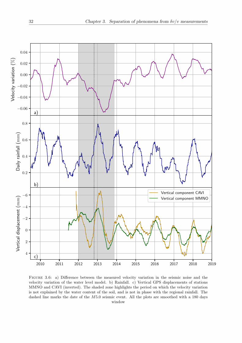
32 Chapter 3. Separation of phenomena from δv/v measurements
−0.06
−0.04
−0.02
0.00
0.02
0.04
Vel
oci
tyva
riat
ion
(%)
a)
0.2
0.4
0.6
0.8
Dai
lyra
infa
ll(mm
)
b)
2010 2011 2012 2013 2014 2015 2016 2017 2018 2019
−6
−4
−2
0
2
4
Ver
tica
ldi
spla
cem
ent
(mm
)
c)
Vertical component CAVI
Vertical component MMNO
Figure 3.6: a) Difference between the measured velocity variation in the seismic noise and thevelocity variation of the water level model. b) Rainfall. c) Vertical GPS displacements of stationsMMNO and CAVI (inverted). The shaded zone highlights the period on which the velocity variationis not explained by the water content of the soil, and is not in phase with the regional rainfall. Thedashed line marks the date of the M5.0 seismic event. All the plots are smoothed with a 180 days
window

3.6. Conclusions 33
N36W follows the same behavior that both the measured and modeled velocity variations,for the whole period recorded with the GPS. This can be explained by the pressure generatedby the water that opens and closes the fractures of the porous media, generating the overalldisplacements registered by the GPS; this behavior is also seen between all the other stationsthat are located in the zone. This confirms our assumption of a poroelastic recharge anddischarge process of the aquifer, upon which we based the water level models. The angleat which this occurs for the couples that involve the station MMNO is always around 36,which is close to the angle of the strike fault of the M5.0 event (24), possibly because at thisdirection the sharp displacement generated by the earthquake is minimized. Moreover, theangles that maximize this expansion-contraction mechanism for the couples that are not closeto the earthquake (namely, VIGG-CAVI, VIGG-SALB, and CAVI-SALB), show interestingdifferences that are possibly related to the shape of the aquifer or local anisotropic behavior.
The subtraction of the predicted velocity variation generated by the water level inside theaquifer from the observed seismic one, reveals a pattern of weaker amplitude that is in phasewith the regional rainfall. We also observe that the vertical displacements of the GPS on thezone are well anti-correlated with the rainfall of the zone. This indicates an elastic behaviorof the zone that happens in parallel with the described poroelastic dynamics: the rainfallgenerates an instantaneous loading over the surface that has a consequence, the subsidenceof the elevation of the zone (therefore the anti-correlation with the vertical GPS) and a smallincrease on the stress of the crust (and consequently an increase of the seismic velocity) thatis registered in the δv/v.
Finally, this procedure highlights a period on which an anomalous velocity drop breaksthe in-phase behavior between the residual seismic velocity and both the rainfall and thevertical GPS. This happens simultaneously with the period of high seismic activity of theregion, which includes theM5.0 event. Therefore, the velocity drop is probably related to thestress release associated with the seismic activity of the zone. This means that our analysisallows us to extract the seismic signature of the tectonic stress release, despite having twoenvironment processes, the elastic and the poroelastic response to the precipitation, workingsimultaneously and dominating the variation of the seismic velocity.

34 Chapter 3. Separation of phenomena from δv/v measurements
3.7 Supplementary information
0.000 0.001 0.002 0.003 0.004 0.005 0.006 0.007
Value of constant k, L.R. model (1/day)
0.0
0.5
1.0
1.5
2.0
2.5
3.0
3.5M
isfi
t(×
10−
3)
Linear reservoir
Torricelli
0.000 0.001 0.002 0.003 0.004 0.005 0.006 0.007Value of constant k′, Torricelli model (
√mm/day)
Figure 3.7: Misfit of each of the model for different values of k

3.7. Supplementary information 35
0.00
0.05
0.10
0.15
0.20
0.25
0.30
Dai
lyra
infa
ll(mm
)
1980 1984 1988 1992 1996 2000 2004 2008 2012 2016
0.00
0.25
0.50
0.75
1.00
1.25
1.50
1.75
Wat
erle
vel
(a.u.)
Linear resevoir
Torricelli
Figure 3.8: Water level estimation from both discharge models along withthe rainfall.
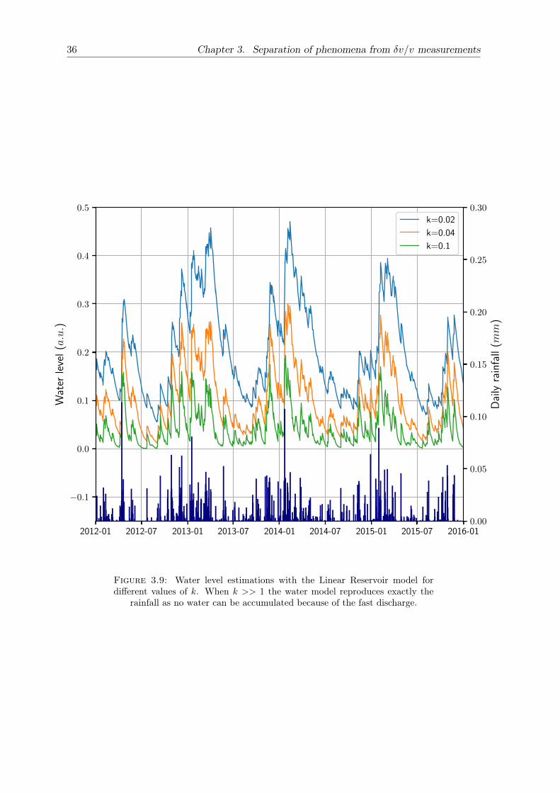
36 Chapter 3. Separation of phenomena from δv/v measurements
2012-01 2012-07 2013-01 2013-07 2014-01 2014-07 2015-01 2015-07 2016-01
−0.1
0.0
0.1
0.2
0.3
0.4
0.5
Wat
erle
vel
(a.u.)
k=0.02
k=0.04
k=0.1
0.00
0.05
0.10
0.15
0.20
0.25
0.30
Dai
lyra
infa
ll(mm
)
Figure 3.9: Water level estimations with the Linear Reservoir model fordifferent values of k. When k >> 1 the water model reproduces exactly the
rainfall as no water can be accumulated because of the fast discharge.

3.7. Supplementary information 37
−4
−2
0
2
Z component station MMNO
−2.5
0.0
2.5 Z component station VIGG
−5
0
5
Z component station CAVI
2010 2011 2012 2013 2014 2015 2016 2017 2018 2019
−5
0
5Z component station SALB
GP
Sd
isp
lace
men
t(mm
)
Figure 3.10: Vertical GPS components smoothed with a 180 days window.The dashed line marks the date of the M5.0 seismic event.

38 Chapter 3. Separation of phenomena from δv/v measurements
2010 2011 2012 2013 2014 2015 2016 2017 2018 2019
−10
0
10
20
30
GP
Sdi
spla
cem
ent
(mm
)
NS station MMNO
NS station VIGG
Figure 3.11: North-South components of the stations VIGG and MMNOshifted towards zero, and their relative displacement shifted around its mean.All the traces are smoothed with a 30 days window. The dashed line marks
the date of the M5.0 seismic event.

3.7. Supplementary information 39
2010 2011 2012 2013 2014 2015 2016 2017 2018 2019
−10
−5
0
5
10
15
GP
Sdi
spla
cem
ent
(mm
)
N36W station MMNO
N36W station VIGG
Figure 3.12: Rotated North-South components of the stations VIGG andMMNO shifted towards zero, and their relative displacement shifted around itsmean. All the traces are smoothed with a 30 days window. The dashed line
marks the date of the M5.0 seismic event.

40 Chapter 3. Separation of phenomena from δv/v measurements
2010 2011 2012 2013 2014 2015 2016 2017 2018 2019
−15
−10
−5
0
5
10
GP
Sdi
spla
cem
ent
(mm
)
EW station MMNO
EW station VIGG
Figure 3.13: East-West components of the stations VIGG and MMNO shiftedtowards zero, and their relative displacement shifted around its mean. All thetraces are smoothed with a 30 days window. The dashed line marks the date
of the M5.0 seismic event.

3.7. Supplementary information 41
2010 2011 2012 2013 2014 2015 2016 2017 2018 2019
−20
−10
0
10
20
GP
Sdi
spla
cem
ent
(mm
)
N126W station MMNO
N126W station VIGG
Figure 3.14: Rotated east-West components of the stations VIGG andMMNO shifted towards zero, and their relative displacement shifted aroundits mean. All the traces are smoothed with a 30 days window. The dashed line
marks the date of the M5.0 seismic event.

42 Chapter 3. Separation of phenomena from δv/v measurements
−50 0 50
Rotation angle (deg)
1.5
2.0
2.5
3.0
3.5
Mis
fit
(%)
×10−3
Figure 3.15: Misfit between the rotated NS relative displacement and thewater level model for different periods.
43
Chapter 4
Coupling between surface and bodywaves
Ludovic Margerin, Andres Barajas, Michel CampilloArticle in published in Geophysical Journal International
In the preceding chapter we studied the influence of different factors on the measurementsof apparent velocity at the surface, and we proposed a way to separate them using alternativesources of data and physical modeling. However, we want to locate the actual perturbationsat depth that generate the phase fluctuations at the surface. This would give us a naturalway of separating the phenomena responsible for those changes and a more insightful visionof the processes in the crust of the Earth. The first step towards that objective is to developa theoretical frame over which we can describe the coupling between surface and body waves,and the energy exchange between them close to the surface. However, developing this modelfor the elastic case is still an open and challenging problem in seismology. In this chapter, wepresent a simpler case, a scalar model in the half-space that includes a particular boundarycondition that gives rise to the natural formation of surface waves. Based on this model wefind fundamental relations of the conversion between surface and body waves and we constructa set of transport equations that will be fundamental for the estimation of the travel-timesensitivity kernel in the next chapter.
4.1 Abstract
To describe the energy transport in the seismic coda, we introduce a system of radiativetransfer equations for coupled surface and body waves in a scalar approximation. Our modelis based on the Helmholtz equation in a half-space geometry with mixed boundary conditions.In this model, Green’s function can be represented as a sum of body waves and surface waves,which mimics the situation on Earth. In a first step, we study the single-scattering problemfor point-like objects in the Born approximation. Using the assumption that the phase ofbody waves is randomized by surface reflection or by interaction with the scatterers, weshow that it becomes possible to define, in the usual manner, the cross-sections for surface-to-body and body-to-surface scattering. Adopting the independent scattering approximation, wethen define the scattering mean free paths of body and surface waves including the couplingbetween the two types of waves. Using a phenomenological approach, we then derive a set ofcoupled transport equations satisfied by the specific energy density of surface and body wavesin a medium containing a homogeneous distribution of point scatterers. In our model, thescattering mean free path of body waves is depth dependent as a consequence of the body-to-surface coupling. We demonstrate that an equipartition between surface and body wavesis established at long lapse-time, with a ratio which is predicted by usual mode countingarguments. We derive a diffusion approximation from the set of transport equations and

44 Chapter 4. Coupling between surface and body waves
show that the diffusivity is both anisotropic and depth dependent. The physical origin ofthe two properties is discussed. Finally, we present Monte-Carlo solutions of the transportequations which illustrate the convergence towards equipartition at long lapse-time as wellas the importance of the coupling between surface and body waves in the generation of codawaves.
4.2 Introduction
In seismology, Radiative Transfer (RT) has been used for more than three decades to charac-terize the scattering and absorption properties of Earth’s crust (see for instance Fehler et al.,1992; Hoshiba, 1993; Carcolé and Sato, 2010; Eulenfeld and Wegler, 2017). Since its intro-duction by Wu (1985) for scalar waves in the stationary regime, RT has been considerablyimproved to bring it in closer agreement with real-world applications. In particular, the cou-pling between shear and compressional waves was developed in a series of papers by Weaver(1990), Turner and Weaver (1994), Yuehua Zeng (1993), Sato (1994b), and Ryzhik, Papan-icolaou, and Keller (1996). The model of Sato (1994b) was applied to data from an activeexperiment by Yamamoto and Sato (2010) and showed impressive agreement between obser-vations and elastic RT theory. For comprehensive introductions to RT, the reader is referredto the review chapter by Margerin (2005) or the monograph of Sato and Fehler (2012).
Parallel to the physical and mathematical developments of the theory, more and morerealistic Monte-Carlo simulations of the transport process were developed over the years.This includes, for example, the treatment of non-isotropic scattering (Abubakirov and Gu-sev, 1990; Hoshiba, 1995; Gusev and Abubakirov, 1996; Jing, Zeng, and Lin, 2014; Sato andEmoto, 2018), velocity and heterogeneity stratification (Hoshiba, 1997; Margerin, Campillo,and Tiggelen, 1998; Yoshimoto, 2000), coupling between shear and compressional waves(Margerin, Campillo, and Van Tiggelen, 2000; Przybilla, Wegler, and Korn, 2009), later-ally varying velocity and scattering structures (Sanborn, Cormier, and Fitzpatrick, 2017).With the growth of computational power, Monte-Carlo simulations opened up new venues forthe application of RT in seismology: imaging of deep Earth heterogeneity (Margerin, 2003;Shearer and Earle, 2004; Mancinelli and Shearer, 2013; “On the frequency dependence andspatial coherence of pkp precursor amplitudes”), mapping of the depth-dependent scatteringand absorption structure of the lithosphere (Mancinelli, Shearer, and Liu, 2016; Takeuchiet al., 2017), modeling of propagation anomalies in the crust (Sens–Schönfelder, Margerin,and Campillo, 2009; Sanborn and Cormier, 2018), P-to-S conversions in the teleseismic coda(Gaebler, Sens-Schönfelder, and Korn, 2015), to cite a few examples only.
Recently, RT has also been applied to the computation of sensitivity kernels for time-lapseimaging methods such as coda wave interferometry (see e.g. Poupinet, Ellsworth, and Frechet,1984; Snieder, 2006; Poupinet, Got, and Brenguier, 2008). Coda Wave Interferometry (CWI)exploits tiny changes of waveforms in the coda to map the temporal variations of seismicproperties in 3-D. The mapping relies on the key concept of sensitivity kernels, which, in theframework of CWI, were introduced by Pacheco and Snieder (2005) in the diffusion regimeand Pacheco and Snieder (2006) in the single-scattering regime. These kernels take the formof spatio-temporal convolutions of the mean intensity in the coda. It was later pointed outby Margerin et al. (2016) that an accurate computation of traveltime sensitivity kernels, validfor an arbitrary scattering order and an arbitrary spatial position, requires the knowledgeof the angular distribution of energy fluxes in the coda. These fluxes, or specific intensities,are directly predicted by the radiative transfer model, which makes it attractive for imagingapplications.

4.2. Introduction 45
In noise-based monitoring (Wegler and Sens-Schönfelder, 2007) -also known as PassiveImage Interferometry (PII)- the virtual sources and receivers are located at the surface ofthe medium so that the early coda is expected to contain a significant proportion of Rayleighwaves. At longer lapse-time, the surface waves couple with body waves and the coda eventuallyreaches an equipartition regime when all the propagative surface and body wave modes areexcited to equal energy (Weaver, 1982; Hennino et al., 2001). Because the volumes exploredby surface and body waves are significantly different, the knowledge of the composition of thecoda wavefield at a given lapse-time in the coda is key to locate accurately the changes atdepth in the crust.
Obermann et al. (2013a) and Obermann et al. (2016) proposed to express the sensitivityof coda waves as a linear combination of the sensitivity of surface and body waves, whosekernels are computed from scalar RT theory in 2-D and 3-D, respectively. The relative contri-bution of the 2-D and 3-D sensitivity kernels at a given lapse-time in the coda is determinedby fitting the traveltime shift predicted by the theory against full wavefield numerical simula-tions in scattering media, where the background seismic velocity is perturbed in a fine layerat a given depth. This method has been validated in the case of 1-D perturbations throughnumerical tests and has the advantage of modeling exactly the complex coupling between sur-face and body waves in heterogeneous media. Furthermore, it can easily incorporate realistictopographies, which is important for the monitoring of volcanoes. The main drawbacks ofthe approach of Obermann et al. (2016) are the numerical cost and the fact that it requires agood knowledge of the scattering properties of the medium, which have to be determined byother methods such as MLTWA (Fehler et al., 1992; Hoshiba, 1993).
This brief overview illustrates that CWI and PII would benefit from a formulation of RTtheory which incorporates the coupling between surface and body waves in a self-consistentway. In the case of a slab bounded by two free surfaces, Trégourès and Van Tiggelen, 2002derived from first principles a quasi 2-D RT equation where the wavefield is expanded onto abasis of Rayleigh, Lamb and Love eigenmodes. Thanks to the normal mode decomposition,this model incorporates the boundary conditions at the level of the wave equation. The energyexchange between surface and body waves is treated by normal mode coupling in the Bornapproximation. A notable advantage of this formulation is the capacity to predict directlythe energy decay in the coda and its parttioning onto different components. The two mainlimitations for seismological applications are the slab geometry, which may not always berealistic and the fact that the disorder should be weak, i.e., the mean free time should belarge compared to the vertical transit time of the waves through the slab.
Zeng (2006) proposed a system of coupled integral equations to describe the exchange ofenergy between surface waves and body waves in the seismic coda. The formalism used bythe author is interesting and bears some similarities with the one developed in this work, al-though we formulate the theory in integro-differential form. A blind spot in the work of Zeng(2006) is the coupling between surface and body waves, which is introduced in an entirely phe-nomenological way and differs significantly from our findings. A very promising investigationof the energy exchange between surface and body waves on the basis of the elastodynamicequations in a half-space geometry was performed by Maeda, Sato, and Nishimura (2008).Using the Born approximation, these authors calculated the scattering coefficients between allpossible modes of propagation in a medium containing random inhomogeneities. The mainlimitation of their theory comes from the fact that the conversion from body to surface wavesis quantified by a non-dimensional coefficient, which makes it difficult to extend their resultsbeyond the single-scattering regime. The authors argue that the absence of a characteristicscale-length for body-to-surface attenuation is a consequence of the fact that all conversionsoccur in approximately one Rayleigh wavelength in the vicinity of the surface.

46 Chapter 4. Coupling between surface and body waves
In this work, we revisit the problem of coupling surface and body waves in a RT frame-work using an approach similar to the one of Maeda, Sato, and Nishimura (2008). Forsimplicity, we limit our investigations to a scalar model based on the Helmholtz equationwith an impedance (or mixed) boundary condition in a half-space geometry. To make thepresentation self-contained, we review the most important features of this particular waveequation. Specifically, we recall that the modes of propagation are composed of body waves,and surface waves whose penetration depth depends on the impedance condition only. Hence,our model mimics the situation on Earth while minimizing the mathematical complexity. Wethen introduce a simple point-scattering model and study its properties in the Born approxi-mation. Using the additional assumption that the surface reflexion randomizes the phase ofthe reflected wave, we are able to derive simple expressions for the scattering mean free pathof both body and surface waves including the coupling between the two. We elaborate on thisresult to establish a set of two coupled RT equations satisfied by the specific energy densityof surface and body waves using a phenomenological approach. Some consequences of oursimple theory are explored, in particular the establishment of a diffusion and equipartitionregime. Monte-Carlo simulations show the potential of the approach to model the transportof energy in the seismic coda from single-scattering to diffusion.
4.3 Scalar wave equation model with surface and body waves
In this section, we present the basic ingredients of our scalar model based on the Helmholtzequation. We describe how an appropriate modification of boundary conditions at the surfaceof a half-space gives rise to the presence of a surface wave. We subsequently present anexpression of the Green’s function and its asymptotic approximation. The concept of densityof states, important for later developments, is recalled. For a thorough treatment of themathematical foundations of our model, the interested reader is refered to the monograph ofHein and Hein R. (2010).
4.3.1 Equation of motion
We consider a 3-D version of the membrane vibration equation in a half-space geometry:
(ρ∂tt − T∆)u(t,R) = 0 (4.1)
where t is time and R is the position vector. It may be further decomposed as R = r + zz(z ≥ 0) with r = xx + yy and (x, y, z) denotes a Cartesian system. In Eq. (4.1) u, ρ and Tmay be thought of as the displacement, the density and the elastic constant of the medium,respectively. The wave Eq. (4.1) is supplemented with the boundary conditions:
(∂z + α)u(t,R)|z=0 = 0
+radiation condition at ∞ (4.2)
The case of interest to us corresponds to α > 0, i.e. when, as recalled below, the boundarycan support a surface wave. Equation (4.1) can be derived by applying Hamilton’s principleto the following Lagrangian density:
L =1
2
[ρ(∂tu(t,R))2 − T (∇u(t,R))2 + αTu(t,R)2δ(z)
](4.3)
Thanks to the last term of the Lagrangian (4.3), which corresponds to a negative elasticpotential energy stored at the surface z = 0, the first B.C. in Eq. (4.2) becomes natural in

4.3. Scalar wave equation model with surface and body waves 47
the sense of variational principles. To make the presentation self-contained, we explain inAppendix 4.8.1 the origin of the delta function in Eq. (4.3) in the simple case of a finite stringwith mixed boundary conditions at one end and free boundary conditions at the other end.
In the case of a harmonic time dependence u ∝ e−iωt (ω > 0), the vibrations are governedby Helmholtz Eq.:
∆u(R) +ω2
c2u(R) = 0 (4.4)
with c =√T/ρ the speed of propagation of the waves in the bulk of the medium. Eq. (4.4)
is complemented with the mixed boundary condition ∂zu+ αu = 0 at z = 0 and an outgoingwave condition at infinity. From (4.3), we can deduce the energy flux density vector J andthe energy density w using the concept of stress-energy tensor (Morse and Ingard, 1986). Forharmonic motions, their average value over a period can be expressed as:
J =− T
2Re iωu∗∇u (4.5)
w =1
4
ρω2|u|2 + T |∇u|2 − αT |u|2δ(z)
(4.6)
In the following section, we recall the consequences of mixed boundary conditions on theHelmoltz Eq., in particular the fact that it gives rise to a surface wave mode.
4.3.2 Eigenfunctions and Green’s function
Due to the translational invariance of the medium, we look for eigen-solutions of Eq. (4.4) inthe form u = ψ(z)eik‖·r with k‖ = (kx, ky, 0). This leads to a self-adjoint eigenvalue problemin the z variable only. For α > 0, part of the spectrum is discrete with eigenfunction :
us(r, z) =√
2αe−αzeik‖·r
2π(4.7)
with k‖ · k‖ − α2 =ω2
c2. The rest of the spectrum forms a continuum of body waves with
normalized eigenfunctions:
ub(r, z) =1
(2π)3/2(e−iqz + r(q)eiqz)eik‖·r, q ≥ 0 (4.8)
with q2 + k‖ · k‖ =ω2
c2and:
r(q) =q + iα
q − iα (4.9)
Note the relations: (1) q = (ω cos j)/c = k cos j with j the incidence angle of the bodywave and (2) |r(q)|2 = 1, i.e., there is total reflection at the surface. For later reference, weintroduce a specific notation for the vertical eigenfunction of body waves:
ψb(n, z) = (e−ikzn·z + r(kn · z)eikzn·z) (4.10)
with n · z = cos j. Note that throughout the paper, we use a hat to denote a unit vector.The surface waves (4.7) and body waves (4.8) are normalized and orthogonal in the sense ofthe scalar product 〈u|v〉 =
∫R3+u(R)∗v(R)d3R, where u and v are arbitrary square integrable
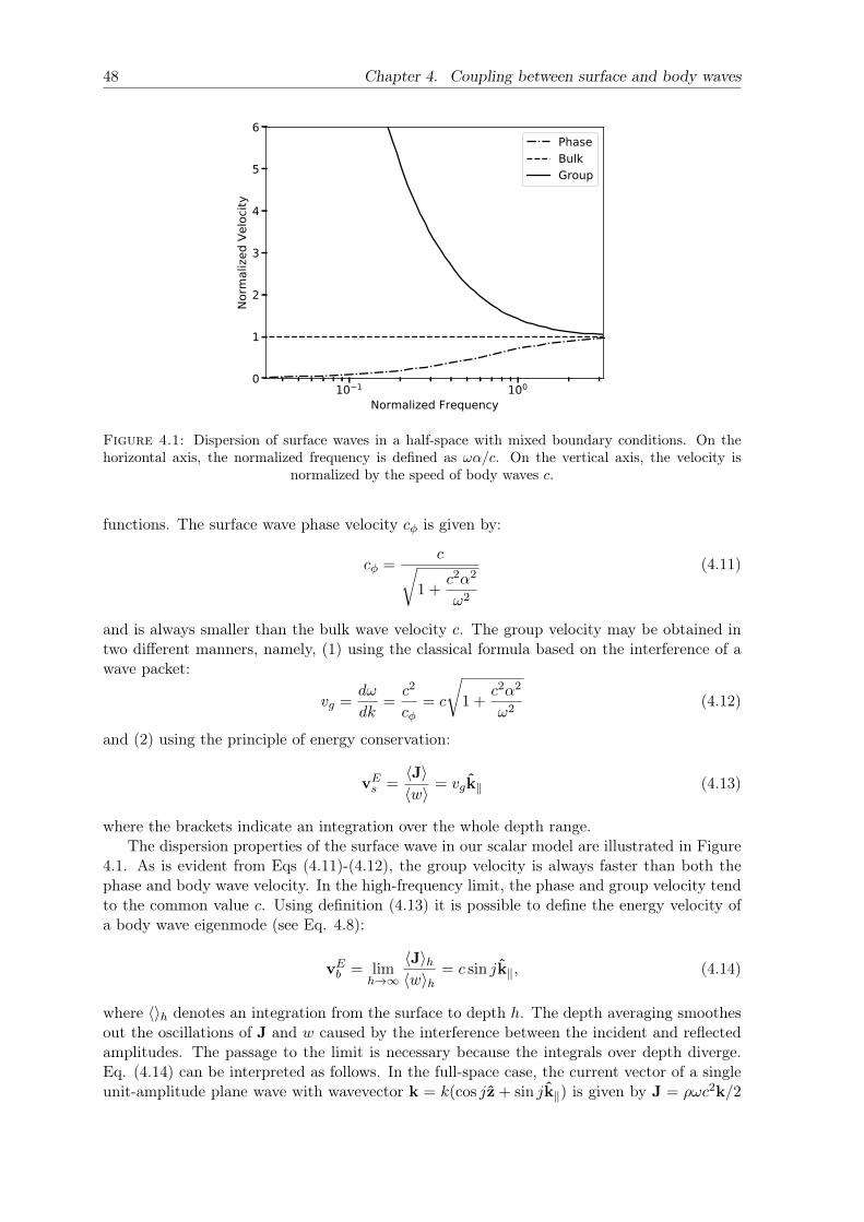
48 Chapter 4. Coupling between surface and body waves
10 1 100
Normalized Frequency
0
1
2
3
4
5
6
Norm
alize
d Ve
locit
y
PhaseBulkGroup
Figure 4.1: Dispersion of surface waves in a half-space with mixed boundary conditions. On thehorizontal axis, the normalized frequency is defined as ωα/c. On the vertical axis, the velocity is
normalized by the speed of body waves c.
functions. The surface wave phase velocity cφ is given by:
cφ =c√
1 +c2α2
ω2
(4.11)
and is always smaller than the bulk wave velocity c. The group velocity may be obtained intwo different manners, namely, (1) using the classical formula based on the interference of awave packet:
vg =dω
dk=c2
cφ= c
√1 +
c2α2
ω2(4.12)
and (2) using the principle of energy conservation:
vEs =〈J〉〈w〉 = vgk‖ (4.13)
where the brackets indicate an integration over the whole depth range.The dispersion properties of the surface wave in our scalar model are illustrated in Figure
4.1. As is evident from Eqs (4.11)-(4.12), the group velocity is always faster than both thephase and body wave velocity. In the high-frequency limit, the phase and group velocity tendto the common value c. Using definition (4.13) it is possible to define the energy velocity ofa body wave eigenmode (see Eq. 4.8):
vEb = limh→∞
〈J〉h〈w〉h
= c sin jk‖, (4.14)
where 〈〉h denotes an integration from the surface to depth h. The depth averaging smoothesout the oscillations of J and w caused by the interference between the incident and reflectedamplitudes. The passage to the limit is necessary because the integrals over depth diverge.Eq. (4.14) can be interpreted as follows. In the full-space case, the current vector of a singleunit-amplitude plane wave with wavevector k = k(cos jz + sin jk‖) is given by J = ρωc2k/2
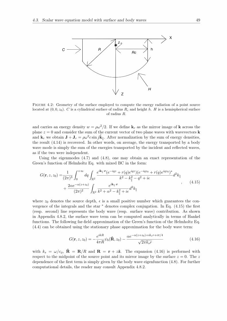
4.3. Scalar wave equation model with surface and body waves 49
Figure 4.2: Geometry of the surface employed to compute the energy radiation of a point sourcelocated at (0, 0, z0). C is a cylindrical surface of radius Rc and height h. H is a hemispherical surface
of radius R.
and carries an energy density w = ρω2/2. If we define kr as the mirror image of k across theplane z = 0 and consider the sum of the current vector of two plane waves with wavevectors kand kr we obtain J + Jr = ρω2c sin jk‖. After normalization by the sum of energy densities,the result (4.14) is recovered. In other words, on average, the energy transported by a bodywave mode is simply the sum of the energies transported by the incident and reflected waves,as if the two were independent.
Using the eigenmodes (4.7) and (4.8), one may obtain an exact representation of theGreen’s function of Helmholtz Eq. with mixed BC in the form:
G(r, z, z0) =1
(2π)3
∫ +∞
0dq
∫R2
eik‖·r(e−iqz + r(q)eiqz)(e−iqz0 + r(q)eiqz0)∗
k2 − k2‖ − q2 + iεd2k‖
+2αe−α(z+z0)
(2π)2
∫R2
eik‖·r
k2 + α2 − k2‖ + iεd2k‖
, (4.15)
where z0 denotes the source depth, ε is a small positive number which guarantees the con-vergence of the integrals and the star ∗ denotes complex conjugation. In Eq. (4.15) the first(resp. second) line represents the body wave (resp. surface wave) contribution. As shownin Appendix 4.8.2, the surface wave term can be computed analytically in terms of Hankelfunctions. The following far-field approximation of the Green’s function of the Helmholtz Eq.(4.4) can be obtained using the stationary phase approximation for the body wave term:
G(r, z, z0) = − eikR
4πRψb(R, z0)−
αe−α(z+z0)+iksr+iπ/4√2πksr
(4.16)
with ks = ω/cφ, R = R/R and R = r + zz. The expansion (4.16) is performed withrespect to the midpoint of the source point and its mirror image by the surface z = 0. The zdependence of the first term is simply given by the body wave eigenfunction (4.8). For furthercomputational details, the reader may consult Appendix 4.8.2.
50 Chapter 4. Coupling between surface and body waves
4.3.3 Source radiation and density of states
We now compute the energy radiated by a point source located at (0, 0, z0). To do so, weintroduce a cylindrical surface C of radius Rc extending from the free surface to a depth hgreater than z0 and large compared to 1/α. We close this surface with a hemispherical cap Hof radius R centered at the surface point (0, 0, 0). The geometry is schematically depicted inFigure 4.2. The energy flux vector (4.5) of the radiated field contains terms that are purelysurface, purely bulk and cross-terms. The contribution of surface waves to the flux across thehemispherical surface is negligible (the error made is exponentially small). The contributionof body waves to the flux across the lateral cylindrical surface is also negligible because thissurface subtends a solid angle which goes to 0 as Rc increases. The cross-terms are negligibleacross the whole surface because the coupled surface/body wave term decays algebraicallyfaster than the surface wave term on the cylindrical surface and exponentially faster than thebody wave term on the hemispherical surface. Hence, we may split the flux of radiated wavesinto a contribution of surface and body waves, respectively.
The energy transported per unit time by body waves through the hemispherical cap H isgiven by:
Eb(z0) =ρω2c
2
∫H|Gb(r, z, z0)|2R2dR
=ρω2c
32π2
∫2π|ψb(R, z0)|2dR,
(4.17)
with Gb the body wave part of Green’s function. In the second line of Eq. (4.17), the integralis over the space directions subtended by the hemispherical cap. (N.B.: strictly speaking, thetotal solid angle is not equal to 2π because one should remove the directions corresponding tothe cylinder. But as noted before, the measure of this set of directions goes to zero as Rc goesto infinity.) The function defined in Eq. (4.17) oscillates with depth around the followingmean value:
〈Eb〉 =ρω2c
8π(4.18)
Here the brackets may have at least 2 different meanings. The most obvious is an averageover depth, as was done in the calculation of the group velocity. But we may also assumethat the surface “scrambles" the phase of the reflected wave φr so that it becomes a randomvariable. In this scenario, the brackets would mean an average over all realizations of therandom reflection process. Upon averaging over phase or depth, the interference patternbetween the incident and reflected wave is smoothed out, so that the two approaches yieldthe same result. Note that the randomization of the phase does not affect energy conservationbecause the incident flux is still totally reflected. In particular, the discussion following theinterpretation of Eq. (4.14) would still be valid. In practice, the assumption that the phaseof the reflected wave is randomized by the surface may not be as unrealistic as it seems.Observations of reflected SH waves by Kinoshita (1993) at borehole stations in Japan indeedsuggest that the reflected field is a distorted version of the incident one. This concurs withthe general view that the subsurface of the Earth is highly heterogeneous at scales that can bemuch smaller than the wavelength and brings support to the idea that aberrating fine layerscould indeed randomize the phase of the reflected wave as we hypothesize. In what follows,the scrambled-phase assumption will be adopted to simplify the treatment of the reflection ofbody waves at the surface.
4.3. Scalar wave equation model with surface and body waves 51
The energy transported per unit time by surface waves through the lateral cylindricalsurface C is given by:
Es(z0) =ρω2vg
2
∫C|Gs(r, z, z0)|2rdφdz
=ρω2vgα
2e−2αz0
4πks
∫ 2π
0dφ
∫ h
0e−2αzdz
=ρωc2α
4e−2αz0
(4.19)
with Gs the surface wave part of Green’s function. Because h is large compared to 1/α theintegral over depth may be performed from 0 to +∞ (the error incurred is exponentiallysmall). We find the depth dependent surface-to-body energy ratio:
R(z0) =Es(z0)〈Eb〉
=2πcα
ωe−2αz0 (4.20)
Formula (4.20) can also be understood in the light of the local density of states ns,b definedas (Sheng, 2006):
ns,b(z0) = − ImGs,b(r, z0, z0)π
∣∣∣∣r=0,z=z0
×dk2s,b(ω)
dω, (4.21)
where ks,b(ω) stands for the wavenumber of surface or body waves. Using the spectral repre-sentation (4.15), one obtains the (exact) formulas:
nb(z0) =ω2
8π2c3
∫2π|ψb(R, z0)|2d2R (4.22)
〈nb〉 =ω2
2πc3(4.23)
ns(z0) =αω
c2e−2αz0 (4.24)
which show that the partitioning of the energy radiated into surface and body waves by thesource R(z0) is given by the ratio of their local density of states ns(z0)/〈nb〉. Finally, we maycompute the partitioning ratio R between the modal density of surface and body waves byintegrating Eq.(4.24) over z and taking the ratio with (4.23). This yields the simple result:
R =
∫ ∞0
ns(z)
〈nb〉dz =
πc
ω(4.25)
where it is to be noted that the modal density ratio R is independent of the scale length αappearing in the mixed boundary condition of the Helmholtz equation. This result could havebeen deduced directly from the dispersion relations of body and surface waves using classicalmode counting arguments (Kittel, 1976). It is worth noting that the local density of states(4.23) is exactly the same as in the case of the Helmholtz equation in full 3-D space. Althoughthe integral in (4.22) is carried over one hemisphere only, each eigenmode ψb is composed ofan incident and a reflected wave, which -on average- doubles its contribution compared to asingle plane wave state. In the next section, we use our knowledge of the Green’s functionto derive the scattering properties of surface and body waves including the coupling betweenthe two modes of propagation.
52 Chapter 4. Coupling between surface and body waves
4.4 Single scattering by a point scatterer
In this section, we calculate the energy radiated by a single scatterer in a half-space geometryfor incident surface or body waves. For simplicity, we restrict our investigations to point scat-terers and employ Born’s approximation. The resulting expressions are simplified followingthe scrambled phase approximation and interpreted in terms of scattering cross-sections.
4.4.1 Scattering of a surface wave
We now consider the following perturbed Helmholtz Eq.:
∆u(r, z) + k2(1 + εa3δ(r)δ(z − zs))u(r, z) = 0 (4.26)
Here a represents the typical linear dimension of the scatterer located at (0, 0, zs) and it isunderstood that ka 1. ε is the local perturbation of inverse squared velocity. Followingthe standard procedure (Snieder, 1986), we look for solutions of Eq. (4.26) of the form:u = u0 +us, where u0(r, z) = e−αz+i
√α2+ω2/c2x is a surface wave eigenmode of the Helmholtz
equation (the incident field) and us is the scattered field. Using the Born approximation, oneobtains:
u(r, z) = u0(r, z)− k2εa3G(r, z, zs)u0(0, zs) (4.27)
Introducing the coupling strength S = k2a3εe−αzs , one may express the energy radiated bythe body waves through the hemispherical cap H (per unit time) as:
U s→b =ρω2S2c
2(4π)2R2
∫2π|ψb(R, zs)|2R2dR. (4.28)
Note that the coupling term S depends on both intrinsic properties of the scatterer -size andstrength of perturbations- as well as on the properties of the incident wave -depth dependenceof eigenfunction and frequency-.
For a unit amplitude surface wave, the vertically-integrated time-averaged energy fluxdensity is given by
|Js| =ρω2vg
4α. (4.29)
The ratio of (4.28) and (4.29) gives the surface-to-body scattering cross-section:
σs→b(zs) =αck4a6ε2e−2αzs
8π2vg
∫2π|ψb(R, zs)|2dR (4.30)
This cross-section has unit of length. In the case where the surface scrambles the phase ofthe reflected wave, we may compute the mean conversion scattering cross-section by takingthe average over the random phase φr.
〈σs→b(zs)〉 =cαk4a6ε2e−2αzs
2πvg(4.31)
Let us remark again that the averaging smoothes out the interference pattern of the bodywave eigenfunction ψb but does not affect the conservation of energy. Furthermore, the aver-aging procedure makes the scattering pattern isotropic since 〈|ψb(R, zs)|2〉 = 2 with an equalcontribution of upgoing and downgoing waves. The computation of the surface-to-surfacescattering cross-section proceeds in a similar way. The surface-wave energy radiated through

4.4. Single scattering by a point scatterer 53
the lateral surface is given by:
U s→s =ρωc2α2S2
4π
∫2π
∫ +∞
0e−2α(z+zs)dφdz
=ρωc2αS2e−2αzs
4
(4.32)
Normalizing the result (4.32) by the incident flux yields the surface-to-surface scattering crosssection:
σs→s(zs) =cα2k3a6ε2e−4αzs
vg, (4.33)
again with unit of length. If we have a collection of point scatterers with volume densityn, we may define a surface wave scattering mean free path using the independent scatteringapproximation as (Lagendijk and Van Tiggelen, 1996; Trégourès and Van Tiggelen, 2002;Maeda, Sato, and Nishimura, 2008):
1
ls=
∫ ∞0
n(σs→s(z) + σs→b(z)
)dz (4.34)
The approximate formula (4.34) neglects all recurrent interactions between the scatterers,which is valid for sufficiently low concentrations of inclusions.
4.4.2 Scattering of body waves
In the case of an incident body wave mode (4.8), the computation of the energy radiated inthe form of body or surface waves can be performed as in the previous section. The definitionof the scattering cross-section, however, is problematic if we stick to the modal description.Indeed, the vertically integrated energy flux density of a body wave mode, as defined in Eq.(4.8), diverges. We must therefore come back to a conventional plane wave description. Wefirst consider the situation where the scatterer is located at a large depth in the half-space.In this case, it appears reasonable to think that the scattering of a body wave mode shouldbe equivalent to the scattering of a plane wave in the full-space case, at least in a sense to bespecified below. To verify the correctness of this assertion, we start by computing the bodywave cross-section in absence of a boundary. Assuming a unit amplitude incident plane waveand using again the Born approximation, one may express the scattered energy as:
Ufull =ρω2c(k2εa3)2
8π, (4.35)
Normalizing the result by the energy flux density of the incident wave:
|Jb| =ρω2c
2(4.36)
we obtain:
σfull =(k2εa3)2
4π(4.37)
In the half-space geometry, the incident wave has the form (4.8). The total energy scatteredin the form of body waves is still given by Eq. (4.28) provided one redefines the couplingconstant as S = k2a3ε|ψb(Ri, zs)|2, where Ri refers to the incidence direction of the bodywave. Eq. (4.28) differs from formula (4.35) as a consequence of the interference betweenthe incident and reflected waves. In the case of a scattering medium, we may expect these
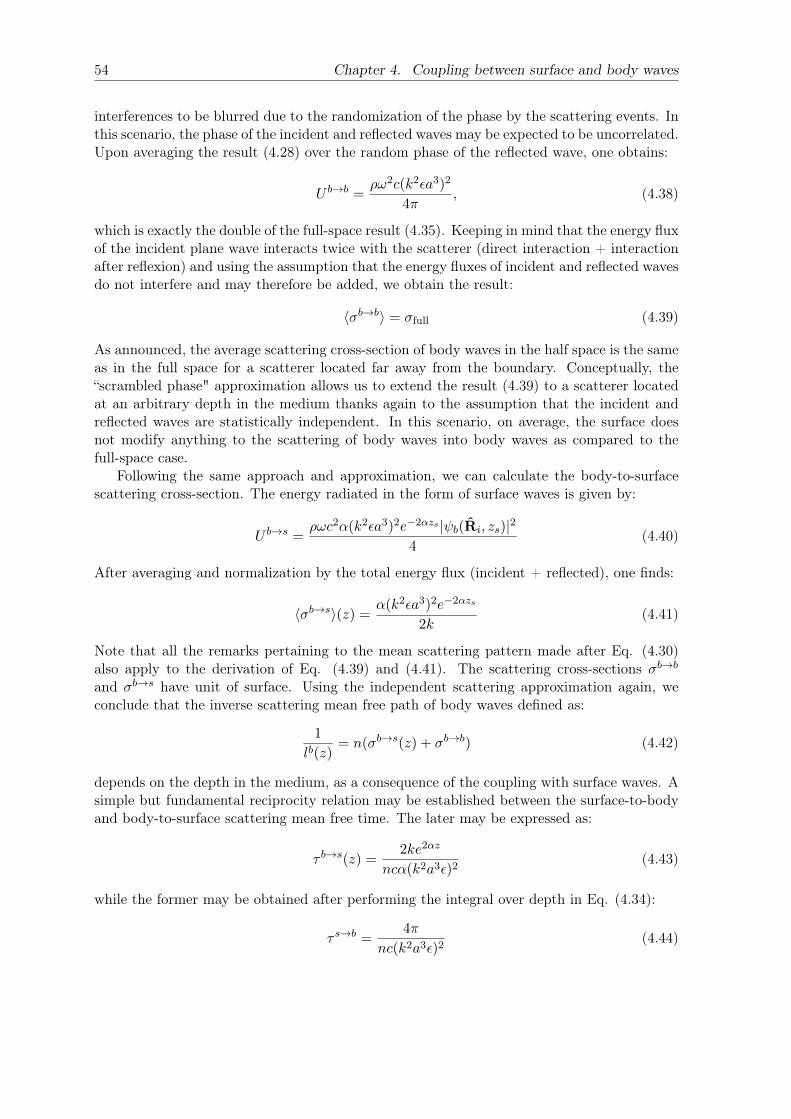
54 Chapter 4. Coupling between surface and body waves
interferences to be blurred due to the randomization of the phase by the scattering events. Inthis scenario, the phase of the incident and reflected waves may be expected to be uncorrelated.Upon averaging the result (4.28) over the random phase of the reflected wave, one obtains:
U b→b =ρω2c(k2εa3)2
4π, (4.38)
which is exactly the double of the full-space result (4.35). Keeping in mind that the energy fluxof the incident plane wave interacts twice with the scatterer (direct interaction + interactionafter reflexion) and using the assumption that the energy fluxes of incident and reflected wavesdo not interfere and may therefore be added, we obtain the result:
〈σb→b〉 = σfull (4.39)
As announced, the average scattering cross-section of body waves in the half space is the sameas in the full space for a scatterer located far away from the boundary. Conceptually, the“scrambled phase" approximation allows us to extend the result (4.39) to a scatterer locatedat an arbitrary depth in the medium thanks again to the assumption that the incident andreflected waves are statistically independent. In this scenario, on average, the surface doesnot modify anything to the scattering of body waves into body waves as compared to thefull-space case.
Following the same approach and approximation, we can calculate the body-to-surfacescattering cross-section. The energy radiated in the form of surface waves is given by:
U b→s =ρωc2α(k2εa3)2e−2αzs |ψb(Ri, zs)|2
4(4.40)
After averaging and normalization by the total energy flux (incident + reflected), one finds:
〈σb→s〉(z) =α(k2εa3)2e−2αzs
2k(4.41)
Note that all the remarks pertaining to the mean scattering pattern made after Eq. (4.30)also apply to the derivation of Eq. (4.39) and (4.41). The scattering cross-sections σb→b
and σb→s have unit of surface. Using the independent scattering approximation again, weconclude that the inverse scattering mean free path of body waves defined as:
1
lb(z)= n(σb→s(z) + σb→b) (4.42)
depends on the depth in the medium, as a consequence of the coupling with surface waves. Asimple but fundamental reciprocity relation may be established between the surface-to-bodyand body-to-surface scattering mean free time. The later may be expressed as:
τ b→s(z) =2ke2αz
ncα(k2a3ε)2(4.43)
while the former may be obtained after performing the integral over depth in Eq. (4.34):
τ s→b =4π
nc(k2a3ε)2(4.44)

4.5. Equation of radiative transfer 55
The ratio between the two quantities is given by:
τ s→b
τ b→s(z)=
2παe−2αz
k= R(z) (4.45)
where Eq. (4.20) has been used. Eq. (4.45) establishes a link between the surface-to-bodyversus body-to-surface conversion rates and the local density of states. In the case of elasticwaves, a similar relation applies (Weaver, 1990; Ryzhik, Papanicolaou, and Keller, 1996): theratio between the P -to-S and S-to-P scattering mean free times is given by the ratio of thedensity of states of P and S waves. As shown in the next section, the relation (4.45) plays akey role in the establishment of an equipartion between surface and body waves.
4.5 Equation of radiative transfer
In this section, we employ standard energy balance arguments to derive a set of coupledequations of RT for surface and body waves in a half-space containing a uniform distributionof point-scatterers. A notable feature of our formulation is the appearance of the penetrationdepth of surface waves as a parameter in the Equations.
4.5.1 Phenomenological derivation
Before we establish the transport equation, a few remarks are in order. It is clear that thetransport of surface wave energy is naturally described by a specific surface energy densityεs(t, r, n) where n is a unit vector in the horizontal plane. The surface energy density ofsurface waves may in turn be defined as:
εs(t, r) =
∫2πεs(t, r, n)dn (4.46)
where the integral is carried over all propagation directions in the horizontal plane. Notethat the εs symbol should not be confused with the strength of fluctuations in Eq. (4.26). Incontrast with surface waves, the transport of body waves is described by a specific volumetricenergy density eb(t, r, k, z) where k is a vector on the unit sphere in 3-D. The volumetricenergy density of body waves is again obtained by integration of the specific energy densityover all propagation directions in 3-D:
Eb(t, r, z) =
∫4πeb(t, r, z, k)dk (4.47)
In the usual formulation of transport equations, energy densities have the same unit (eithersurfacic or volumetric). In order to treat on the same footing surface and body waves, weintroduce the following volumetric energy density of surface waves as:
es(t, r, z, n) = 2αεs(t, r, n)e−2αz (4.48)
It is clear that upon integration of es over depth, one recovers the surface density εs. Theexponential decay of the surface wave energy density is directly inherited from the modalshape and implies that the coupling between surface and body waves mostly occurs within askin layer of typical thickness 1/2α. For future reference, we introduce the following notation:
Es(t, r, z) =
∫2πes(t, r, z, n)dn (4.49)

56 Chapter 4. Coupling between surface and body waves
to represent the volumetric energy density of surface waves, consistent with Eq. (4.47). Notethat the total energy density at a given point will be defined as the sum (Eb(t, r, z)+Es(t, r, z)),thereby implying the incoherence between the two types of waves.
With this definition of the surface wave energy density, the phenomenological derivationof the radiative transport equation follows exactly the same procedure as in the multi-modalcase (Turner and Weaver, 1994). A beam of energy followed along its path around directionni is affected by (1) conversion of energy into other propagating modes and/or deflection intoother propagation directions no 6= ni; (2) a gain of energy thanks to the reciprocal process:a wave with mode i propagating in direction ni can be converted into a wave with modeo propagating in direction no by scattering. In the general case of finite size scatterers wemay anticipate scattering to be anisotropic. To describe such an angular dependence of thescattering process, we may introduce normalized phase functions pi→o(no, ni). The phasefunction may be understood as the probability that a wave of mode i propagating in directionni be converted into a wave of mode o propagating in direction no. To be interpretableprobabilistically, its integral over all outgoing directions (no) should equal 1. Note that inaddition to the incoming and outgoing propagation directions, the phase function may alsodepend on the depth in the medium as a consequence of the presence of the surface. In thecase of point scatterers, this complexity disappears thanks to the scrambled phase assumptionand will therefore not be considered in our formalism.
A detailed local balance of energy yields the following system of coupled transport equa-tions:
(∂t + vgn · ∇) es(t, r, z, n) =− es(t, r, z, n)
τ s+
1
τ s→s
∫2πps→s(n, n′)es(t, r, z, n′)dn′
+1
τ b→s(z)
∫4πpb→s(n, k′; z)eb(t, r, z, k
′)dk′ + ss(t, r, z, n)(∂t + ck · ∇
)eb(t, r, z, k) =− eb(t, r, z, k)
τ b(z)+
1
τ b→b
∫4πpb→b(k, k′)eb(t, r, z, k
′)dk′
+1
τ s→b
∫2πps→b(k, n′)es(t, r, z, n′)dn′ + sb(t, r, z, n)
(4.50)
where the terms ss,b represent sources of surface and body waves. To take into account thereflection of body waves at the surface, the sytem (4.50) is supplemented with the followingboundary condition for the energy density eb:
eb(t, r, 0, k) = eb(t, r, 0, kr) (4.51)
where kr is the mirror image of the incident direction k (k · z < 0) across the horizontal planez = 0. The boundary condition (4.51) is compatible with the assumption that the incidentand reflected waves are statistically independent.
In the simple case of a unit point-like source at depth z0, the terms ss and sb are givenrespectively by:
ss(t, r, z, n) =2αR(z0)e
−2αzδ(r)
2π(1 +R(z0))
sb(t, r, z, k) =δ(z − z0)δ(r)
4π(1 +R(z0))
(4.52)
where R(z0) is the energy partitioning ratio defined in Eq. (4.20). Note that ss follows the
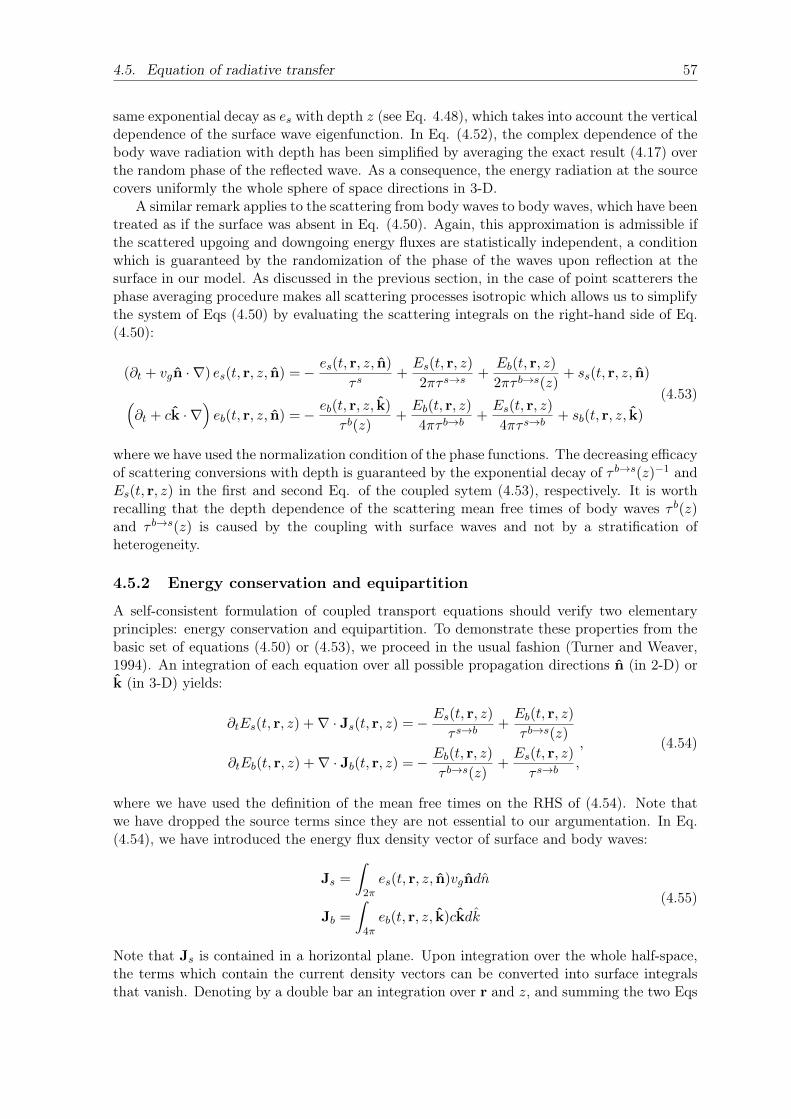
4.5. Equation of radiative transfer 57
same exponential decay as es with depth z (see Eq. 4.48), which takes into account the verticaldependence of the surface wave eigenfunction. In Eq. (4.52), the complex dependence of thebody wave radiation with depth has been simplified by averaging the exact result (4.17) overthe random phase of the reflected wave. As a consequence, the energy radiation at the sourcecovers uniformly the whole sphere of space directions in 3-D.
A similar remark applies to the scattering from body waves to body waves, which have beentreated as if the surface was absent in Eq. (4.50). Again, this approximation is admissible ifthe scattered upgoing and downgoing energy fluxes are statistically independent, a conditionwhich is guaranteed by the randomization of the phase of the waves upon reflection at thesurface in our model. As discussed in the previous section, in the case of point scatterers thephase averaging procedure makes all scattering processes isotropic which allows us to simplifythe system of Eqs (4.50) by evaluating the scattering integrals on the right-hand side of Eq.(4.50):
(∂t + vgn · ∇) es(t, r, z, n) =− es(t, r, z, n)
τ s+Es(t, r, z)
2πτ s→s+Eb(t, r, z)
2πτ b→s(z)+ ss(t, r, z, n)(
∂t + ck · ∇)eb(t, r, z, n) =− eb(t, r, z, k)
τ b(z)+Eb(t, r, z)
4πτ b→b+Es(t, r, z)
4πτ s→b+ sb(t, r, z, k)
(4.53)
where we have used the normalization condition of the phase functions. The decreasing efficacyof scattering conversions with depth is guaranteed by the exponential decay of τ b→s(z)−1 andEs(t, r, z) in the first and second Eq. of the coupled sytem (4.53), respectively. It is worthrecalling that the depth dependence of the scattering mean free times of body waves τ b(z)and τ b→s(z) is caused by the coupling with surface waves and not by a stratification ofheterogeneity.
4.5.2 Energy conservation and equipartition
A self-consistent formulation of coupled transport equations should verify two elementaryprinciples: energy conservation and equipartition. To demonstrate these properties from thebasic set of equations (4.50) or (4.53), we proceed in the usual fashion (Turner and Weaver,1994). An integration of each equation over all possible propagation directions n (in 2-D) ork (in 3-D) yields:
∂tEs(t, r, z) +∇ · Js(t, r, z) =− Es(t, r, z)
τ s→b+Eb(t, r, z)
τ b→s(z)
∂tEb(t, r, z) +∇ · Jb(t, r, z) =− Eb(t, r, z)
τ b→s(z)+Es(t, r, z)
τ s→b,
, (4.54)
where we have used the definition of the mean free times on the RHS of (4.54). Note thatwe have dropped the source terms since they are not essential to our argumentation. In Eq.(4.54), we have introduced the energy flux density vector of surface and body waves:
Js =
∫2πes(t, r, z, n)vgndn
Jb =
∫4πeb(t, r, z, k)ckdk
(4.55)
Note that Js is contained in a horizontal plane. Upon integration over the whole half-space,the terms which contain the current density vectors can be converted into surface integralsthat vanish. Denoting by a double bar an integration over r and z, and summing the two Eqs

58 Chapter 4. Coupling between surface and body waves
of the system (4.54) leaves us with:
∂t
(¯Es(t) + ¯Eb(t)
)= 0 (4.56)
which demonstrates the conservation of energy.In order to prove the existence of equipartition, we integrate each Eq. of the system (4.54)
over the horizontal plane and from the surface to a finite depth h, typically large comparedto the surface wave penetration depth. To simplify the derivation, we assume that at z = hlies a perfectly reflecting surface through which no energy can flow. Because αh 1, themedium may be still be considered as a half-space in the treatment of surface waves. Thisleads us to:
∂t¯Es(t) =−
¯Es(t)
τ s→b+
∫ h
0
Eb(t, z)
τ b→s(z)dz
∂t
∫ h
0Eb(t, z)dz =−
∫ h
0
Eb(t, z)
τ b→s(z)dz +
¯Es(t)
τ s→b,
(4.57)
where the single bar denotes an integration over r only. Note that ¯Es is the total energyof surface waves (up to an exponentially small correction term), in contrast with Eb whichrepresents the body wave energy per unit depth. Our goal is not to solve the system of Eq.(4.57) in its full generality but rather to exhibit an equipartition solution. In this regime, weexpect the distribution of body wave energy to become independent of depth. Hence we lookfor solutions of the system (4.57) of the form:( ¯Es(t)
Eb(t, z)
)=
( ¯E0s
E0b
)e−λt (4.58)
Reporting the ansatz (4.58) into the integro-differential system (4.57), one arrives at a linearand homogeneous system of algebraic equations. A non-zero solution is obtained only if thedeterminant of the sytem vanishes which implies:
λ
(λ− 1
τ s→b− 1
h
∫ h
0
dz
τ b→s(z)
)= 0 (4.59)
One of the solutions is given by λ = 0 which corresponds to the asymptotic equipartitionstate such as:
¯E0s
E0b
=
∫ h
0
τ s→b
τ b→s(z)dz ≈
∫ +∞
0R(z)dz = R (4.60)
where Eq. (4.25) and (4.45) have been used, and the depth integral is again extended to+∞ thanks to the assumption αh 1. Eq. (4.60) illustrates that the ratio between theenergy density of surface and body waves approaches the ratio of their density of states Rat long lapse-time. Note that the energy density is not perfectly homogenized spatially, evenat equipartition, as a consequence of the decay of the surface wave eigenfunction with depth.This may be related to the depth-dependence of the density of states near the boundary(see e.g. Hennino et al., 2001). The result (4.60) could have been predicted using the usualconcept of equipartition which states that when filtered around a narrow frequency band, allthe propagating modes of a diffuse field should be excited to equal energy (Weaver, 1982). Inthe case where the medium is unbounded at depth, there will be a flux of energy across thelower boundary z = h which vanishes as the lapse-time increases. As demonstrated throughnumerical simulations later in this paper, equipartition also sets in in this configuration,though probably more slowly than in the slab geometry.

4.5. Equation of radiative transfer 59
4.5.3 Diffusion Approximation
Having established the existence of an equipartition state, we now derive a diffusion approxi-mation for the transport process. At the outset, it should be clear that the volumetric energydensity Es may not be the solution of a diffusion equation because it exhibits a decay withdepth which is inherited from the modal shape and therefore independent of the scatteringproperties. To circumvent the difficulty, we derive a closed diffusion equation for Eb fromwhich we subsequently deduce the energy density of surface waves. To simplify the calcula-tions, we assume that the scattering is isotropic. Proceeding in the usual fashion, we expandthe specific energy density into its first two angular moments (Akkermans and Montambaux,2007):
es(t, r, z, n) =Es(t, r, z)
2π+
Js(t, r, z) · nπ
eb(t, r, z, k) =Eb(t, r, z)
4π+
3Jb(t, r, z) · k4π
. (4.61)
Multiplying, respectively, the first and second line of Eq. (4.53) by the unit vectors n andk, integrating over all possible directions and employing the moment expansion (4.61), weobtain the following set of Equations:
∂tJs(t, r, z)
vg+vg2∇‖Es(t, r, z) =− Js(t, r, z)
vgτ s
∂tJb(t, r, z)
c+c
3∇Eb(t, r, z) =− Jb(t, r, z)
cτ b
, (4.62)
where ∇‖ denotes the gradient operator in the horizontal plane. Note that the expansions(4.61) are used only to evaluate the integral of the gradient on the left-hand side of the RTEquation. All other terms follow directly either from the definition of the energy flux densityvector or the assumption of isotropic scattering. Our final approximation consists in neglectingthe derivative of the current vector with respect to time which yields the equivalent of Ohm’slaw for the mutiply-scattered waves:
Js(t, r, z) =−Ds∇‖Es(t, r, z)Jb(t, r, z) =−Db(z)∇Eb(t, r, z)
(4.63)
where the following notations have been introduced:
Ds =v2gτ
s
2
Db(z) =c2τ b(z)
3
(4.64)
Note that the total reflection condition (4.51) imposes that there is no net flux of body wavesacross the surface z = 0. To make progress, we now invoke the equipartition principle to fixthe ratio between the energy densities of surface and body waves:
Es(t, r, z)
Eb(t, r, z)= R(z) (4.65)
in agreement with Eq. (4.60). This allows us to express the total energy flux as:
J = Jb + Js = −(R(z)Ds +Db(z))∇‖Eb(t, r, z) +Db(z)z∂zEb(t, r, z) (4.66)

60 Chapter 4. Coupling between surface and body waves
which may be interpreted as a generalization of Ohm’s law for diffuse waves. Eq (4.66)demonstrates that the coupling between surface and body waves renders the energy transportboth depth-dependent and anisotropic. It is worth emphasizing that depth-dependence andanisotropy are caused neither by specific orientations/shapes of the scatterers nor by the non-homogeneity of the statistical properties. As further discussed below, these properties stemfrom the coupling between body and surface wave modes.
The conservation equation for the total energy E = Es + Eb excited by a point source att = 0 is obtained by taking the sum of the set of Eqs (4.54):
∂tE(t, r, z) +∇ · J(t, r, z) = δ(t)δ(z − z0)δ(r), (4.67)
where the right-hand side now contains the source term with z0 the source depth. Makinguse of Eqs (4.65) and (4.63), we obtain the following diffusion-like equation verified by thebody wave energy density:
∂tEb(t, r, z)−∇‖ ·(Db(z) +R(z)Ds
1 +R(z)∇‖Eb(t, r, z)
)− 1
1 +R(z)∂z (Db(z)∂zEb(t, r, z)) =
δ(t)δ(r)δ(z − z0)1 +R(z0)
(4.68)
The last term on the left-hand side of Eq. (4.68) differs from the traditional form for thediffusion model due to the (1 +R(z))−1 factor in front of the derivative operators. Actually,this difference is purely formal as may be shown by the change of variable z → z′ where z′ isdefined as:
z′ =∫ z
0(1 +R(x))dx,
=z +π
k
(e−2αz − 1
) (4.69)
where Eq. (4.20) has been used. In the new variables, Eq. (4.68) may be rewritten as:
∂tE′b(t, r, z
′)−∇‖ ·(D‖(z
′)∇‖E′b(t, r, z′))− ∂z′
(D⊥(z′)∂z′E
′b(t, r, z
′))
= δ(t)δ(r)δ(z′ − z′0)(4.70)
In Eq. (4.70), we have introduced the notations E′b(t, r, z′) = Eb(t, r, z), z′0 =
∫ z00 (1+R(x))dx,
as well as the following definitions of the horizontal and vertical diffusivities:
D‖(z′) =
Db(z) +R(z)Ds
1 +R(z)
D⊥(z′) =Db(z)(1 +R(z))
(4.71)
Hence, a simple change of scale in the vertical direction reduces Eq.(4.68) to the conventionaldiffusion Eq. (4.70). Note that the (1 + R(z0))
−1 factor on the right-hand side has beenabsorbed by the change of variable (4.69).
We explore the consequences of Eq. (4.71) by first considering the case z′ →∞. Accordingto Eq. (4.69), this implies z′ ≈ z. Since the partitioning ratio R(z) goes to zero at large depthin the medium, Eq. (4.71) indicates that the vertical and horizontal diffusivities become equaland the diffusion tensor isotropic. Furthermore, because the coupling between surface andbody waves is negligible at large depth, its magnitude tends to the constant value Dbulk
b =c2τ b→b/3, as expected on physical grounds. In other words, the diffusion process at depth isgoverned by a simple 3-D diffusion equation for body waves with diffusion constantDbulk
b . This
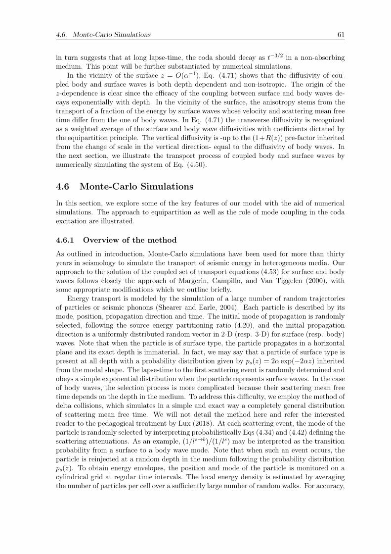
4.6. Monte-Carlo Simulations 61
in turn suggests that at long lapse-time, the coda should decay as t−3/2 in a non-absorbingmedium. This point will be further substantiated by numerical simulations.
In the vicinity of the surface z = O(α−1), Eq. (4.71) shows that the diffusivity of cou-pled body and surface waves is both depth dependent and non-isotropic. The origin of thez-dependence is clear since the efficacy of the coupling between surface and body waves de-cays exponentially with depth. In the vicinity of the surface, the anisotropy stems from thetransport of a fraction of the energy by surface waves whose velocity and scattering mean freetime differ from the one of body waves. In Eq. (4.71) the transverse diffusivity is recognizedas a weighted average of the surface and body wave diffusivities with coefficients dictated bythe equipartition principle. The vertical diffusivity is -up to the (1+R(z)) pre-factor inheritedfrom the change of scale in the vertical direction- equal to the diffusivity of body waves. Inthe next section, we illustrate the transport process of coupled body and surface waves bynumerically simulating the system of Eq. (4.50).
4.6 Monte-Carlo Simulations
In this section, we explore some of the key features of our model with the aid of numericalsimulations. The approach to equipartition as well as the role of mode coupling in the codaexcitation are illustrated.
4.6.1 Overview of the method
As outlined in introduction, Monte-Carlo simulations have been used for more than thirtyyears in seismology to simulate the transport of seismic energy in heterogeneous media. Ourapproach to the solution of the coupled set of transport equations (4.53) for surface and bodywaves follows closely the approach of Margerin, Campillo, and Van Tiggelen (2000), withsome appropriate modifications which we outline briefly.
Energy transport is modeled by the simulation of a large number of random trajectoriesof particles or seismic phonons (Shearer and Earle, 2004). Each particle is described by itsmode, position, propagation direction and time. The initial mode of propagation is randomlyselected, following the source energy partitioning ratio (4.20), and the initial propagationdirection is a uniformly distributed random vector in 2-D (resp. 3-D) for surface (resp. body)waves. Note that when the particle is of surface type, the particle propagates in a horizontalplane and its exact depth is immaterial. In fact, we may say that a particle of surface type ispresent at all depth with a probability distribution given by ps(z) = 2α exp(−2αz) inheritedfrom the modal shape. The lapse-time to the first scattering event is randomly determined andobeys a simple exponential distribution when the particle represents surface waves. In the caseof body waves, the selection process is more complicated because their scattering mean freetime depends on the depth in the medium. To address this difficulty, we employ the method ofdelta collisions, which simulates in a simple and exact way a completely general distributionof scattering mean free time. We will not detail the method here and refer the interestedreader to the pedagogical treatment by Lux (2018). At each scattering event, the mode of theparticle is randomly selected by interpreting probabilistically Eqs (4.34) and (4.42) defining thescattering attenuations. As an example, (1/ls→b)/(1/ls) may be interpreted as the transitionprobability from a surface to a body wave mode. Note that when such an event occurs, theparticle is reinjected at a random depth in the medium following the probability distributionps(z). To obtain energy envelopes, the position and mode of the particle is monitored on acylindrical grid at regular time intervals. The local energy density is estimated by averagingthe number of particles per cell over a sufficiently large number of random walks. For accuracy,

62 Chapter 4. Coupling between surface and body waves22 L. Margerin et al.
0 10 20 30 40Time
0
2
4
6
8
10
¯ Es/
Eb
Shallow
Deep
Asymptote
0 10 20 30 40Time
103
102
101
¯ Es/
¯ Eb
Shallow
Deep
/ t1/2
Figure 2. Local and global evolution of energy partitioning for a shallow (solid line) and a deep (dash-
dotted line) source in a heterogeneous half-space filled with point scatterers. The horizontal time scale
is the mean free time for surface wave scattering. The penetration depth of surface waves is ↵1 = 1
km and the angular frequency is ! = 2 Hz. The shallow and deep source are located, respectively,
at depth ↵1 and 5↵1. (Left): Temporal evolution of the ratio between the total energy of surface
waves ( ¯Es) and the energy density of body waves integrated over a horizontal plane (Eb). The body
wave energy is evaluated at the surface and averaged over a depth z = 1km. The asymptote (left) is
the prediction of Eq. (25). (Right) Temporal evolution of the ratio between the total energy of surface
( ¯Es) and body waves ( ¯Eb). The dotted line shows an algebraic t1/2 decay.
uniformly distributed random vector in 2-D (resp. 3-D) for surface (resp. body) waves. Note
that when the particle is of surface type, the particle propagates in a horizontal plane and its
exact depth is immaterial. In fact, we may say that a particle of surface type is present at all
depth with a probability distribution given by ps(z) = 2↵ exp(2↵z) inherited from the modal
shape. The lapse-time to the first scattering event is randomly determined and obeys a simple
0 2 4 6 8 10Depth
0.00005
0.00010
0.00015
0.00020
0.00025
0.00030
0.00035
Ene
rgy
Den
sity
t = 1
t = 2
t = 5
t = 10 t = 15
Figure 3. Horizontally-averaged energy density of body waves Eb as a function of depth in a heteroge-
neous half-space filled point scatterers. The energy is averaged over a depth range z = ↵1/5 = 0.2km
and the horizontal axis shows the depth normalized by ↵1. The solid and dashed line correspond to
a shallow source (z0 = 1km) and a deep source (z0 = 5km), respectively. The lapse time in the coda
in mean free time unit is indicated on the right of the corresponding curves.
Figure 4.3: Local and global evolution of energy partitioning for a shallow (solid line) and a deep(dash-dotted line) source in a heterogeneous half-space filled with point scatterers. The horizontaltime scale is the mean free time for surface wave scattering. The penetration depth of surface wavesis α−1 = 1 km and the angular frequency is ω = 2π Hz. The shallow and deep source are located,respectively, at depth α−1 and 5α−1. (Left): Temporal evolution of the ratio between the totalenergy of surface waves ( ¯Es) and the energy density of body waves integrated over a horizontal plane(Eb). The body wave energy is evaluated at the surface and averaged over a depth ∆z = 1km. Theasymptote (left) is the prediction of Eq. (4.25). (Right) Temporal evolution of the ratio between thetotal energy of surface ( ¯Es) and body waves ( ¯Eb). The dotted line shows an algebraic t−1/2 decay.
it is important that the cells be relatively small compared to the shortest mean free path inthe medium.
4.6.2 Numerical results
Figure 4.3 illustrates the striking difference between the global and local partitioning of theseismic energy into surface and body waves. The following parameters have been employed inthe simulation: α = 1km−1, c = 3km/s and τ s→s = 20s, τ s→b = 30s, τ b→b = 30s, τ b→s(z) =10 exp(2z)s. Note that in our model the group velocity of surface waves vg ≈ 3.32km/s isslightly faster than the speed of propagation of body waves. Two source depths are considered:a relatively shallow one (z0 = 1km) and a deep one (z0 = 5km), which radiate approximately29% and 0.01% energy as surface waves, respectively.
On the left, we show the temporal evolution of the ratio between the total energy ofsurface waves ¯Es (see the remarks before Eq. 4.56 for a reminder of the notations), and thehorizontally-integrated energy density of body waves Eb at the surface z = 0, averaged overa depth range ∆z = 1km. Hence, the ratio ¯Es/Eb has unit of inverse length. Independentof the source depth, we find that the partitioning of the energy density at the surface -intosurfacic energy of surface waves and volumetric energy of body waves- converges toward theprediction of equipartition theory, at long lapse-time in the coda (see Eq. 4.25 and 4.60).This numerical result confirms that the analysis of equipartition given in the previous sectionin slab geometry extends to the half-space geometry. Furthermore, we find that the surface-to-body energy ratio overshoots the prediction of equipartition theory for the two sources atshort lapse-time, by a factor which decreases with the source depth z0.
The stabilization of the local energy density ratio of surface and body waves at the surfaceof the half-space is to be contrasted with the evolution of the global partitioning of the energyinto surface and body wave modes. Figure 4.3 (right) shows that after a few mean free times,

4.6. Monte-Carlo Simulations 63
0 2 4 6 8 10Depth
0.00005
0.00010
0.00015
0.00020
0.00025
0.00030
0.00035
Ene
rgy
Den
sity
←− t = 1
←− t = 2
←− t = 5
←− t = 10←− t = 15
Figure 4.4: Horizontally-averaged energy density of body waves Eb as a function of depth in aheterogeneous half-space filled with point scatterers. The energy is averaged over a depth range∆z = α−1/5 = 0.2km and the horizontal axis shows the depth normalized by α−1. The solid anddashed lines correspond to a shallow source (z0 = 1km) and a deep source (z0 = 5km), respectively.The lapse time in the coda in mean free time unit is indicated on the right of the corresponding curves.
most of the energy is carried in the form of body waves in the medium. The Figure alsosuggests that the global transfer of energy from surface waves to body waves occurs at a rateproportional to t−1/2 at long lapse-time.
Further insight into the equipartition process is offered in Figure 4.4, where we show thedepth dependence of the horizontally-averaged body wave energy density at different lapse-time in the coda. All the parameters of the simulation are the same as in Figure 4.3, exceptfor the much finer spatial resolution ∆z = α−1/5 = 0.2 km, which allows us to track processesthat occur in the skin layer where the coupling between surface and body waves occurs. Weobserve that after roughly 10 mean free times, the depth distribution of body wave energybecomes homogeneous over a depth range at least as large as 10α−1, independent of the sourcedepth. This simulation therefore confirms the theoretical analysis performed in slab geometry.The homogenization of the energy of body waves is a dynamic process: the energy densityof surface waves increases exponentially near the surface, thereby generating a larger amountof body-wave converted energy; this process is compensated by the exponential increase ofthe conversion rate from body to surface waves, which eventually yields an equilibrium. Notethat the total energy density does not homogenize with depth, due to the exponential decayof the surface wave eigenfunction with depth.
In Figure 4.5 and 4.7, we illustrate in greater details the multiple-scattering process byshowing snapshots of the surfacic and volumetric energy densities εs(t, r) and Eb(t, r, z)|z=0
at regular time intervals ∆t = 1τ s starting at a lapse time t = 0.8τ s for a shallow (z0 = 1km)and a deep (z0 = 5km) source, respectively. The scattering parameters are the same as inFigure 4.3 and the energy is averaged over a range of epicentral distance ∆r = 5km and depth∆z = 5km. We use a double horizontal axis on Figures 4.5-4.7 to show simultaneously theepicentral distance in kms and in units of mean free path. Note that in the case of body waves,we take the value of the mean free path in the bulk of the medium τ b→b. For comparison,we show in Figure 4.6, snapshots of energy density of surface waves and body waves whenthe coupling between the two is deactivated. In the case of surface waves, this amounts to

64 Chapter 4. Coupling between surface and body waves
0 50 100 150 200 250 300 350 400Distance (km)
10 9
10 8
10 7
10 6
10 5
10 4
Ener
gy D
ensit
y
0 2 4 6 8 10Distance (mfp)
0 50 100 150 200 250 300 350 400Distance (km)
10 9
10 8
10 7
10 6
10 5
Ener
gy D
ensit
y
0 1 2 3 4Distance (mfp)
Figure 4.5: Snapshots of the energy density of surface waves εs (left) and of the volumetric energydensity of body waves Eb (right) at the surface of a heterogeneous half-space filled with point scatterersin the case of a shallow source (z0 = α−1). The horizontal axes are in units of the scattering meanfree path of surface waves (left, top), body waves (right, top) and in kms (bottom). For body waves,we take the mean free path value in the bulk of the medium (z →∞). The energy is averaged over
cylindrical shells of width ∆r = 5km and deph ∆z = 5km.
0 50 100 150 200 250 300 350 400Distance (km)
10 9
10 8
10 7
10 6
10 5
10 4
Ener
gy D
ensit
y
0 2 4 6 8 10Distance (mfp)
0 50 100 150 200 250 300 350 400Distance (km)
10 9
10 8
10 7
10 6
10 5
Ener
gy D
ensit
y
0 1 2 3 4Distance (mfp)
Figure 4.6: Same as Figure 4.5 but the coupling between surface and body waves has been deacti-vated. See text for further explanations.

4.6. Monte-Carlo Simulations 65
0 50 100 150 200 250 300 350 400Distance (km)
10 9
10 8
10 7
10 6
10 5
10 4
Ener
gy D
ensit
y
0 2 4 6 8 10Distance (mfp)
0 50 100 150 200 250 300 350 400Distance (km)
10 9
10 8
10 7
10 6
10 5
Ener
gy D
ensit
y
0 1 2 3 4Distance (mfp)
Figure 4.7: Snapshots of the energy density of surface waves εs (left) and of the volumetric energydensity of body waves Eb (right) at the surface of a heterogeneous half-space filled with point scatterersin the case of a deep source (z0 = 5α−1). The horizontal axes are in units of the scattering meanfree path of surface waves (left, top), body waves (right, top) and in kms (bottom). For body waves,we take the mean free path value in the bulk of the medium (z → ∞). The energy is averaged over
cylindrical shells of width ∆r = 5km and depth ∆z = 5km.
0 50 100 150 200 250 300 350 400Distance (km)
2
4
6
8
10
Scat
terin
g Or
der
0 2 4 6 8 10Distance (mfp)
0 50 100 150 200 250 300 350 400Distance (km)
2
4
6
8
10
Scat
terin
g Or
der
0 2 4 6 8 10Distance (mfp)
Figure 4.8: Contribution of the different orders of scattering to the energy envelopes of surface wavesshown in Figure 4.5 (left, solid lines) and 4.7 (right, solid lines). Snapshots of the mean scatteringorder are represented as a function of the distance from the source. For reference, the dashed lineshow the same distribution for a conventional transport model in 2-D. The horizontal axes are in units
of the scattering mean free path of surface waves (top) and in kms (bottom).
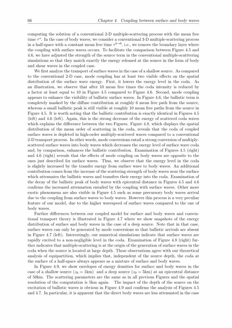
66 Chapter 4. Coupling between surface and body waves
computing the solution of a conventional 2-D multiple-scattering process with the mean freetime τ s. In the case of body waves, we consider a conventional 3-D multiple-scattering processin a half-space with a constant mean free time τ b→b, i.e., we remove the boundary layer wherethe coupling with surface waves occurs. To facilitate the comparison between Figure 4.5 and4.6, we have adjusted the strength of the source term in the conventional multiple-scattteringsimulations so that they match exactly the energy released at the source in the form of bodyand shear waves in the coupled case.
We first analyze the transport of surface waves in the case of a shallow source. As comparedto the conventional 2-D case, mode coupling has at least two visible effects on the spatialdistribution of the surface wave energy. First, it lowers the energy level in the coda. Asan illustration, we observe that after 10 mean free times the coda intensity is reduced bya factor at least equal to 10 in Figure 4.5 compared to Figure 4.6. Second, mode couplingappears to enhance the visibility of ballistic surface waves. In Figure 4.6, the ballistic term iscompletely masked by the diffuse contribution at roughly 6 mean free path from the source,whereas a small ballistic peak is still visible at roughly 10 mean free paths from the source inFigure 4.5. It is worth noting that the ballistic contribution is exactly identical in Figures 4.5(left) and 4.6 (left). Again, this is the strong decrease of the energy of scattered coda waveswhich explains the difference between the two Figures. Figure 4.8, which displays the spatialdistribution of the mean order of scattering in the coda, reveals that the coda of coupledsurface waves is depleted in high-order multiply-scattered waves compared to a conventional2-D transport process. In other words, mode conversions entail a strong conversion of multiply-scattered surface waves into body waves which decreases the energy level of surface wave codaand, by comparison, enhances the ballistic contribution. Examination of Figures 4.5 (right)and 4.6 (right) reveals that the effects of mode coupling on body waves are opposite to theones just described for surface waves. Thus, we observe that the energy level in the codais slightly increased by the transfer energy from surface wave to body waves. An additionalcontribution comes from the increase of the scattering strength of body waves near the surfacewhich attenuates the ballistic waves and transfers their energy into the coda. Examination ofthe decay of the ballistic peak of body waves with epicentral distance in Figures 4.5 and 4.6confirms the increased attenuation entailed by the coupling with surface waves. Other moreexotic phenomena are also visible in Figure 4.5 such as some precursory body waves arrivaldue to the coupling from surface waves to body waves. However this process is a very peculiarfeature of our model, due to the higher wavespeed of surface waves compared to the one ofbody waves.
Further differences between our coupled model for surface and body waves and conven-tional transport theory is illustrated in Figure 4.7 where we show snapshots of the energydistribution of surface and body waves in the case of a deep source. Note that in that case,surface waves can only be generated by mode conversions so that ballistic arrivals are absentin Figure 4.7 (left). Interestingly, our numerical simulations indicate that surface waves arerapidly excited to a non-negligible level in the coda. Examination of Figure 4.8 (right) fur-ther indicates that multiple-scattering is at the origin of the generation of surface waves in thecoda when the source is located at large depth. These observations agree with our theoreticalanalysis of equipartition, which implies that, independent of the source depth, the coda atthe surface of a half-space always appears as a mixture of surface and body waves.
In Figure 4.9, we show envelopes of energy densities for surface and body waves in thecase of a shallow source (z0 = 1km) and a deep source (z0 = 5km) at an epicentral distanceof 50km. The scattering parameters are the same as in all previous Figures and the spatialresolution of the computation is 5km again. The impact of the depth of the source on theexcitation of ballistic waves is obvious in Figure 4.9 and confirms the analysis of Figures 4.5and 4.7. In particular, it is apparent that the direct body waves are less attenuated in the case
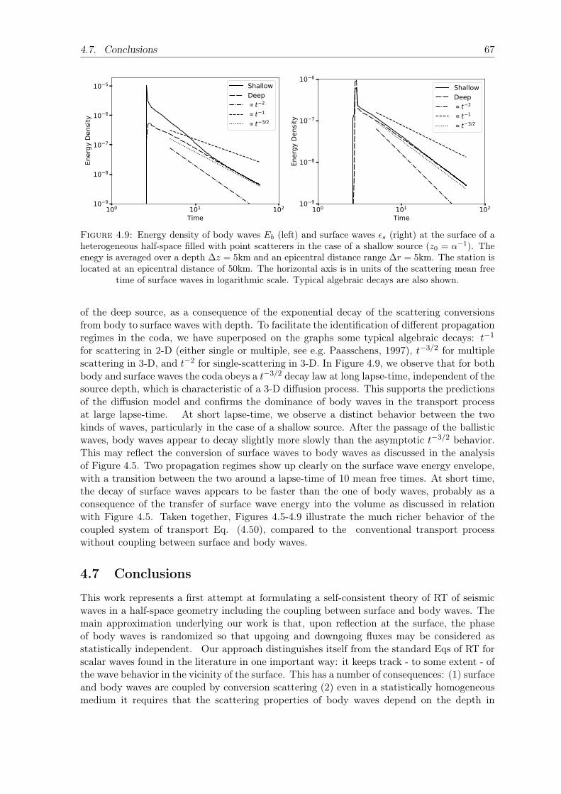
4.7. Conclusions 67
100 101 102
Time
10 9
10 8
10 7
10 6
10 5En
ergy
Den
sity
ShallowDeep
t 2
t 1
t 3/2
100 101 102
Time
10 9
10 8
10 7
10 6
Ener
gy D
ensit
y
ShallowDeep
t 2
t 1
t 3/2
Figure 4.9: Energy density of body waves Eb (left) and surface waves εs (right) at the surface of aheterogeneous half-space filled with point scatterers in the case of a shallow source (z0 = α−1). Theenegy is averaged over a depth ∆z = 5km and an epicentral distance range ∆r = 5km. The station islocated at an epicentral distance of 50km. The horizontal axis is in units of the scattering mean free
time of surface waves in logarithmic scale. Typical algebraic decays are also shown.
of the deep source, as a consequence of the exponential decay of the scattering conversionsfrom body to surface waves with depth. To facilitate the identification of different propagationregimes in the coda, we have superposed on the graphs some typical algebraic decays: t−1
for scattering in 2-D (either single or multiple, see e.g. Paasschens, 1997), t−3/2 for multiplescattering in 3-D, and t−2 for single-scattering in 3-D. In Figure 4.9, we observe that for bothbody and surface waves the coda obeys a t−3/2 decay law at long lapse-time, independent of thesource depth, which is characteristic of a 3-D diffusion process. This supports the predictionsof the diffusion model and confirms the dominance of body waves in the transport processat large lapse-time. At short lapse-time, we observe a distinct behavior between the twokinds of waves, particularly in the case of a shallow source. After the passage of the ballisticwaves, body waves appear to decay slightly more slowly than the asymptotic t−3/2 behavior.This may reflect the conversion of surface waves to body waves as discussed in the analysisof Figure 4.5. Two propagation regimes show up clearly on the surface wave energy envelope,with a transition between the two around a lapse-time of 10 mean free times. At short time,the decay of surface waves appears to be faster than the one of body waves, probably as aconsequence of the transfer of surface wave energy into the volume as discussed in relationwith Figure 4.5. Taken together, Figures 4.5-4.9 illustrate the much richer behavior of thecoupled system of transport Eq. (4.50), compared to the conventional transport processwithout coupling between surface and body waves.
4.7 Conclusions
This work represents a first attempt at formulating a self-consistent theory of RT of seismicwaves in a half-space geometry including the coupling between surface and body waves. Themain approximation underlying our work is that, upon reflection at the surface, the phaseof body waves is randomized so that upgoing and downgoing fluxes may be considered asstatistically independent. Our approach distinguishes itself from the standard Eqs of RT forscalar waves found in the literature in one important way: it keeps track - to some extent - ofthe wave behavior in the vicinity of the surface. This has a number of consequences: (1) surfaceand body waves are coupled by conversion scattering (2) even in a statistically homogeneousmedium it requires that the scattering properties of body waves depend on the depth in

68 Chapter 4. Coupling between surface and body waves
the medium. Furthermore, the reciprocity relation between the surface-to-body vs body-to-surface mean free times plays a prominent role in the establishment of an equipartition regimewith a ratio that conforms to the predictions of standard mode counting arguments. Besidesequipartition, a notable outcome of our RT equations is the anisotropy of the diffusivityof seismic waves, due to the difference in scattering properties and wave velocities of bodyand surface waves. We also show that our RT Eqs are operational, in the sense that they arereadily amenable to numerical solutions by Monte-Carlo simulations. These simulations couldbe used in the future to study in more details the dynamics of equipartition, in particular,how the equipartition time varies as a function of the ratio between the penetration depth ofsurface waves and the scattering mean free path for body-to-surface wave coupling.
Before becoming a viable alternative to current approaches, our theory needs to be testedand improved. In the future, we plan to address the following issues: (1) Evaluate theimpact of neglecting the interference between upgoing and downgoing body waves on thescattering cross-section and, if possible, go beyond this approximation. (2) Extend the theoryto more realistic finite size scatterers and more general spatial distributions of scatterers. (3)Incorporate polarization effects for elastic waves at a free surface. (4) Absorption of energy isalso a very important mechanism of attenuation, which has been entirely neglected in this workfor simplicity. Because the sub-surface of the Earth is thought to be very strongly attenuatingdue to the widespread presence of fluids, we may expect dissipation to affect more severelysurface waves than body waves. In turn, this may modify the partitioning of the energy in thecoda as was previously shown by Margerin, Van Tiggelen, and Campillo (2001) in the case ofcoupled S and P waves. Special efforts should be devoted to this important topic before ourformalism can be applied to real seismic data.
4.8 Supplementary information
4.8.1 Variational formulation for mixed boundary conditions
Here, we recall briefly on a simple one-dimensional example how mixed boundary conditions ofthe type used in Eq. (4.2) can be incorporated into a variational formulation. The interestedreader will find further details and more examples in the classic book by Gelfand and Fomin(1963), after which our treatment is modeled. For simplicity we consider a vibrating stringof density ρ, tension T and length L. For the moment, we do not specify the boundaryconditions. The total kinetic energy stored in the string at time t is given by:
T [u](t) =
∫ L
0ρ(∂tu(x, t))2dx, (4.72)
where u denotes the displacement field. The instantaneous potential energy stored in thestring may be expressed as
V [u](t) =
∫ L
0T (∂xu(x, t))2dx (4.73)
According to Hamilton’s principle, among all possible displacement fields, the one that satisfiesthe actual equations of motion should make the following action integral:
I[u] =
∫ t2
t1
(T − V )[u](t)dt (4.74)
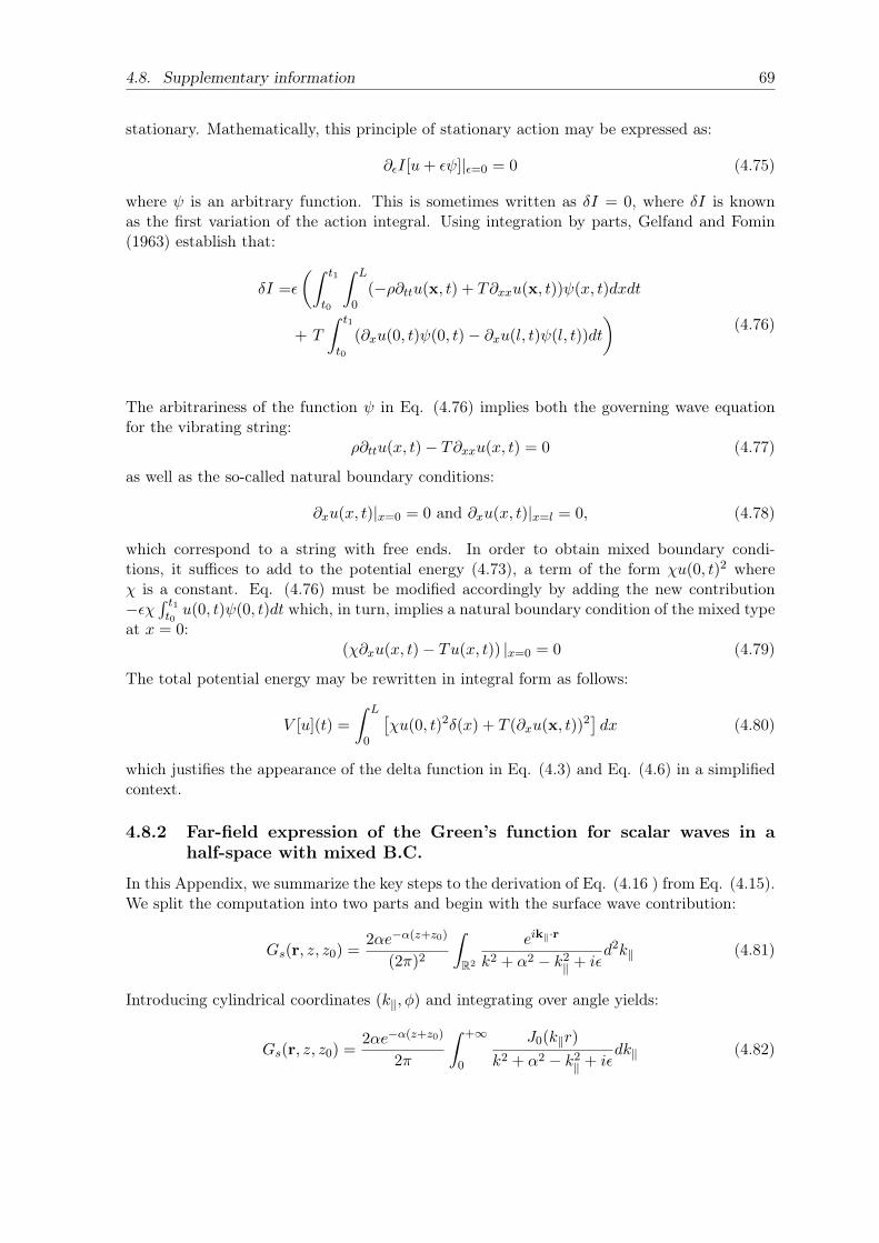
4.8. Supplementary information 69
stationary. Mathematically, this principle of stationary action may be expressed as:
∂εI[u+ εψ]|ε=0 = 0 (4.75)
where ψ is an arbitrary function. This is sometimes written as δI = 0, where δI is knownas the first variation of the action integral. Using integration by parts, Gelfand and Fomin(1963) establish that:
δI =ε
(∫ t1
t0
∫ L
0(−ρ∂ttu(x, t) + T∂xxu(x, t))ψ(x, t)dxdt
+ T
∫ t1
t0
(∂xu(0, t)ψ(0, t)− ∂xu(l, t)ψ(l, t))dt
)(4.76)
The arbitrariness of the function ψ in Eq. (4.76) implies both the governing wave equationfor the vibrating string:
ρ∂ttu(x, t)− T∂xxu(x, t) = 0 (4.77)
as well as the so-called natural boundary conditions:
∂xu(x, t)|x=0 = 0 and ∂xu(x, t)|x=l = 0, (4.78)
which correspond to a string with free ends. In order to obtain mixed boundary condi-tions, it suffices to add to the potential energy (4.73), a term of the form χu(0, t)2 whereχ is a constant. Eq. (4.76) must be modified accordingly by adding the new contribution−εχ
∫ t1t0u(0, t)ψ(0, t)dt which, in turn, implies a natural boundary condition of the mixed type
at x = 0:(χ∂xu(x, t)− Tu(x, t)) |x=0 = 0 (4.79)
The total potential energy may be rewritten in integral form as follows:
V [u](t) =
∫ L
0
[χu(0, t)2δ(x) + T (∂xu(x, t))2
]dx (4.80)
which justifies the appearance of the delta function in Eq. (4.3) and Eq. (4.6) in a simplifiedcontext.
4.8.2 Far-field expression of the Green’s function for scalar waves in ahalf-space with mixed B.C.
In this Appendix, we summarize the key steps to the derivation of Eq. (4.16 ) from Eq. (4.15).We split the computation into two parts and begin with the surface wave contribution:
Gs(r, z, z0) =2αe−α(z+z0)
(2π)2
∫R2
eik‖·r
k2 + α2 − k2‖ + iεd2k‖ (4.81)
Introducing cylindrical coordinates (k‖, φ) and integrating over angle yields:
Gs(r, z, z0) =2αe−α(z+z0)
2π
∫ +∞
0
J0(k‖r)
k2 + α2 − k2‖ + iεdk‖ (4.82)

70 Chapter 4. Coupling between surface and body waves
where J0 denotes the standard Bessel function of order 0. Using the same trick as in Aki andRichards (2002, Chapter 6), we extend the wavenumber integral over the whole k‖ axis usingthe Hankel function of the first kind instead of the Bessel function:
Gs(r, z, z0) =αe−α(z+z0)
2π
∫ +∞
−∞
H(1)0 (k‖r)
k2 + α2 − k2‖ + iεdk‖ (4.83)
In the last step, we employ the residue theorem by closing the contour in the upper half ofthe complex plane with a semi-circle of radius R → +∞ and note the presence of pole atk‖ =
√k2 + α2 + iη, (η → 0+). Thanks to the exponential decay of the integrand, the integral
on the semi-circle vanishes which yields:
Gs(r, z, z0) =−iα2π
e−α(z+z0)H(1)0 (√k2 + α2r). (4.84)
The result (4.84) is exact. The far-field approximation (4.16) follows by application of stan-dard asymptotic expansions to the Hankel function.
The computation of the body wave contribution can also be split into two parts:
Gb(r, z, z0) =1
(2π)3
∫ +∞
0dq
∫R2
eik‖·r(e−iqz + r(q)eiqz)(e−iqz0 + r(q)eiqz0)∗
k2 − k2‖ − q2 + iεd2k‖
=1
(2π)3
∫ +∞
−∞dq
∫R2
eiq(z−z0)eik‖·r
k2 − k2‖ − q2 + iεd2k‖
+1
(2π)3
∫ +∞
−∞dq
∫R2
r(q)eiq(z+z0)eik‖·r
k2 − k2‖ − q2 + iεd2k‖
=G∞(r, z, z0) +Gr(r, z, z0)
(4.85)
where the unitarity of the reflection coefficient has been used and the q integral has beenextended from −∞ to +∞ thanks to the relation r(q)∗ = r(−q). The first term in the secondequality of (4.85) may be recognized as the full-space solution to the Helmholtz Eq.:
G∞(r, z, z0) =1
(2π)3
∫ +∞
−∞dq
∫R2
eiq(z−z0)eik‖·r
k2 − k2‖ − q2 + iεd2k‖
=− eikR0
4πR0,
(4.86)
where R0 =√r2 + (z − z0)2. The second term in the second equality of (4.85) represents the
waves reflected at the surface:
Gr(r, z, z0) =1
(2π)3
∫ +∞
−∞dq
∫R2
r(q)eiq(z+z0)eik‖·r
k2 − k2‖ − q2 + iεd2k‖ (4.87)
The computation of this integral may be attacked in exactly the same way as we did for thesurface wave term Gs to obtain:
Gr(r, z, z0) =−i8π
∫ +∞
−∞r(q)eiq(z+z0)H
(1)0 (√k2 − q2r)dq, (4.88)
To approximate this last integral in the far-field of the source, we first remark that for |q| > kthe cylindrical waves are evanescent so that we may legitimately take −k and +k as integration

4.8. Supplementary information 71
limits. We next make use of the far-field expansion of the Hankel function to obtain thefollowing oscillatory integral representation:
Gr(r, z, z0) ≈−i8π
√2
πr
∫ +k
−k
r(q)eiq(z+z0)+i√k2−q2r−iπ/4√
k2 − q2dq (4.89)
Further noting that the derivative of the phase term:
φ(q) = q(z + z0) +√k2 − q2r (4.90)
vanishes at :q0 =
k(z + z0)
R′0(4.91)
with R′0 =√r2 + (z + z0)2, we apply the stationary phase formula to obtain after some
straightforward algebra:
Gr(r, z, z0) ≈ −r(q0)e
ikR′0
4πR′0. (4.92)
This term may be interpreted as the contribution of the image point of the source with astrength given by the reflection coefficient evaluated at an incidence angle corresponding tothe specularly reflected ray connecting the source to the detection point (see Eq. 4.91). Tocomplete the far-field approximation, we first note the following expansions: R0 = R−z0z/R+o(1/R), R′0 = R + z0z/R + o(1/R) where R =
√r2 + z2. Neglecting all terms smaller than
1/R for the amplitude, all terms smaller than z0/R for the phase and further approximatingq0 as kz/R, formula (4.16) is recovered.

73
Chapter 5
Sensitivity Kernels
Andres Barajas, Ludovic Margerin, Michel CampilloArticle in preparation
A change in the properties of the crust can generate a perturbation in the propagationvelocity of the seismic waves. The phase perturbations of the waveforms registered at thesurface depend on the position of this property change. The connection between the twois the sensitivity kernel. Therefore, if we want to localize perturbations at depth we mustestimate the sensitivity kernel for the model presented in the previous section: this is themain objective of this chapter. To this end, we first study the changes that generate in thescalar surface wave velocity perturbation in the medium. Later, we extend the travel-timesensitivity kernels theory so it incorporates the propagation and detection and surface andbody waves. Then, based on these results and in the radiative transfer equations obtained inthe preceding chapter, we estimate the sensitivity kernel for body and surface waves. Althoughthe theory presented here is general for the scalar case, we restrict ourselves for simplicity to adepth description of the sensitivity. Furthermore, thinking in the eventual application of theseresults to the case study analyzed in chapter 3 where we make measurements from a singlestation, the estimation of the sensitivity kernel is done for the autocorrelation configuration,it means, with the source and the receiver located in the same location.
5.1 Introduction
The heterogeneities present in the crust interact with the passing seismic waves and scatterthem in multiple directions. This phenomenon is directly related to the formation of the codawave which contains information about the strength and properties of this interaction. Thefirst study in this direction was done by Aki (1969) where he defines for the first time thecoda wave and he defines his principal characteristics, and later use it to estimate specificproperties of the region (Aki, 1973) and to analyze the attenuation properties related tothe structure of the Earth (Sciences, Aki, and Chouet, 1975). More studies followed thatshowed that the fluctuations in the amplitude and phase of the scattered waves enable theidentification of small variations in the properties of the crust (Poupinet, Ellsworth, andFrechet, 1984; Ratdomopurbo and Poupinet, 1995; Schaff and Beroza, 2004). The estimationof these changes from the continuous seismic noise field is one of the fundamental principlesof passive image interferometry monitoring which have shown to be effective in detectingvelocity variations in fault zones (Wegler and Sens-Schönfelder, 2007; Brenguier et al., 2008a),in volcanoes (Sens-Schönfelder and Wegler, 2006), or as a consequence of a diverse number ofmeteorological phenomena (Meier, Shapiro, and Brenguier, 2010; Wang et al., 2017; Hillers,Campillo, and Ma, 2014).
The phase differences changes generated in the coda depend on the location of the per-turbation and the time that the seismic field has to sample it, or in other words, with the

74 Chapter 5. Sensitivity Kernels
lapse time. This means that it is possible to locate the perturbation in the crust with theinformation registered at the surface at different times. Coda wave interferometry establishesthe link between the two through the introduction of the sensitivity kernels by Pacheco andSnieder (2005) for the diffusive wave state, and Pacheco and Snieder (2006) for the singlescattering case. The sensitivity kernel is a travel-time density function that shows the mostprobable sectors through which a wave would pass when going from the source to the receiverin a given lapse time. The kernel can be calculated as a convolution of the probabilities of theparticle traveling between the source, the receiver, and each part of the medium around themthat is sampled by the waves (Pacheco and Snieder, 2005). Each of these probabilities canbe interpreted physically as the intensity received at one point of space after a unitary pulsewas emitted from another (Margerin et al., 2016). This is the reason why the estimation ofthe sensitivity pass through the calculation or use of known Green’s functions and solutionsof the transport equation in different dimensions (Paasschens, 1997; Sato and Fehler, 2012).Later (Margerin et al., 2016) demonstrated the importance of the directionality of the seis-mic field in the first stages of the system which implied that an analyses of the sensitivitybased only in the energy intensities was insufficient; to solve it, they developed the sensitivitykernels through specific intensities overcoming with this the restrictions on the propagationregime that was previously limited to the extreme cases as a diffusive or a single-scatteringassumptions, and extending the theory toward anisotropic scattering events.
The sensitivity kernels have been used to localize perturbations in numerical simulations(Planes et al., 2015; Kanu and Snieder, 2015), in a concrete sample (Larose et al., 2010), orgenerated by changes in the medium preceding volcanic eruptions (Lesage, Reyes-Dávila, andArámbula-Mendoza, 2014; Obermann et al., 2013b). The coupling between body and surfacewaves has remained one challenging factor to the development of the sensitivity kernels in a3-D halfspace that is the usual setting for most seismic applications. Obermann et al. (2013a)and Obermann et al. (2016) approached this problem by expressing the sensitivity as a linearcombination of two independent sensitivities, one for surface and another for body waves, witha controlling factor mediating between them that changes with time, and that is estimatedthrough full wavefield numerical simulations. This factor helps to recreate predominance ofsurface and body wave sensitivities at different lapse times. This method has been extendedto localize small scale perturbations in the medium (Obermann et al., 2019).
Recently, Margerin, Bajaras, and Campillo (2019) developed a new scalar model thatintegrates naturally body and surface waves, making it possible to find the different meanfree paths and times between the two modes and therefore, to establish the radiative transferequations of the system. Based on this model, we reformulate the sensitivity equations froma probabilistic point of view to include the two types of propagation and estimate themstatistically through a series of Monte Carlo simulations. This allows us to obtain the travel-time density distributions between the two modes of propagation, for different depths in a3-D half-space medium. In parallel, we estimate the phase perturbations in the surface wavesas a consequence of a perturbation in the medium and integrate it with the results of thesimulations to obtain the sensitivity kernel of the system. We compare the performance ofthis kernel with previous works and analyze its most important features.
5.2 Scalar model
We begin with a quick overview of the scalar model developed by Margerin, Bajaras, andCampillo, 2019. First, we state the wave equation in a 3-D half-space
(ρ∂tt − T∆)u(t, r, z) = 0 (5.1)
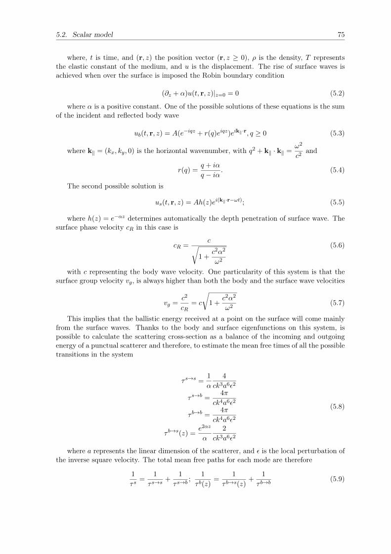
5.2. Scalar model 75
where, t is time, and (r, z) the position vector (r, z ≥ 0), ρ is the density, T representsthe elastic constant of the medium, and u is the displacement. The rise of surface waves isachieved when over the surface is imposed the Robin boundary condition
(∂z + α)u(t, r, z)|z=0 = 0 (5.2)
where α is a positive constant. One of the possible solutions of these equations is the sumof the incident and reflected body wave
ub(t, r, z) = A(e−iqz + r(q)eiqz)eik‖·r, q ≥ 0 (5.3)
where k‖ = (kx, ky, 0) is the horizontal wavenumber, with q2 + k‖ · k‖ =ω2
c2and
r(q) =q + iα
q − iα. (5.4)
The second possible solution is
us(t, r, z) = Ah(z)ei(k‖·r−ωt); (5.5)
where h(z) = e−αz determines automatically the depth penetration of surface wave. Thesurface phase velocity cR in this case is
cR =c√
1 +c2α2
ω2
(5.6)
with c representing the body wave velocity. One particularity of this system is that thesurface group velocity vg, is always higher than both the body and the surface wave velocities
vg =c2
cR= c
√1 +
c2α2
ω2(5.7)
This implies that the ballistic energy received at a point on the surface will come mainlyfrom the surface waves. Thanks to the body and surface eigenfunctions on this system, ispossible to calculate the scattering cross-section as a balance of the incoming and outgoingenergy of a punctual scatterer and therefore, to estimate the mean free times of all the possibletransitions in the system
τ s→s =1
α
4
ck3a6ε2
τ s→b =4π
ck4a6ε2
τ b→b =4π
ck4a6ε2
τ b→s(z) =e2αz
α
2
ck3a6ε2
(5.8)
where a represents the linear dimension of the scatterer, and ε is the local perturbation ofthe inverse square velocity. The total mean free paths for each mode are therefore
1
τ s=
1
τ s→s+
1
τ s→b;
1
τ b(z)=
1
τ b→s(z)+
1
τ b→b(5.9)
76 Chapter 5. Sensitivity Kernels
The dependence of τ b→s on the depth is directly related to the surface wave eigenfuntionwhich changes the probabilities of a scattering event for a body wave depending on its locationrelative to the surface. The ratio between the energy of surface waves and the depth-integratedenergy of body waves generated by a point source:
R(z) =τ s→b
τ b→s(z)=
2πcα
ωe−2αz. (5.10)
The transport of energy of body waves can be described in terms of the specific volumetricenergy density eb(t, r, z,k) where k is a vector on the unit sphere in 3-D. The integration ofthis specific density over a solid angle gives us the volumetric energy density
Eb(t, r, z) =
∫4πeb(t, r, z, k)dk (5.11)
On the other hand, the transport of surface waves can be described in terms of the specificsurface energy density εs(t, r,n) where n is a unit vector in the horizontal plane. To be ableto describe the system through the formulation of transport equations, it is necessary to haveenergy densities of equal dimensions; for this reason, is introduced the specific volumetricenergy density of surface waves
es(t, r, z,n) = 2αεs(t, r,n)e−2αz (5.12)
which integrated over depths give us back the specific surface density εs(t, r,n). Usingthis new specific volumetric density is now possible to define a volumetric energy density ofsurface wave
Es(t, r, z) =
∫2πes(t, r, z, n)dn (5.13)
The total energy density at a point in the medium will be the sum of the energy densitiesof body and surface waves Eb(t, r, z) +Es(t, r, z), which is supported by the orthogonality oftheir representative eigenfunctions.
From these definitions are constructed the radiative transport equations. The scatteringprocess is assumed to be isotropic and the increase and decay of intensity are stated in termsof the conversion between all the possible modes
(∂t + vgn · ∇) es(t, r, z, n) =− es(t, r, z, n)
τ s+Es(t, r, z)
2πτ s→s
+Eb(t, r, z)
2πτ b→s(z)+ ss(t, r, z, n)(
∂t + ck · ∇)eb(t, r, z, n) =− eb(t, r, z, k)
τ b(z)+Eb(t, r, z)
4πτ b→b
+Es(t, r, z)
4πτ s→b+ sb(t, r, z, k)
(5.14)
where the terms ss,b represent sources of surface and body waves, which are given in termsof the energy partitioning ratio
ss(t, r, z, n) =2αR (z0) e
−2αzδ(r)
2π (1 +R (z0))
sb(t, r, z, k) =δ (z − z0) δ(r)
4π (1 +R (z0))
(5.15)
5.3. Penetration depth of the surface wave 77
5.3 Penetration depth of the surface wave
One of the fundamental characterizing parameters of the interaction between body and surfacewaves is the penetration depth of the surface waves. For this reason, finding an equivalencebetween the scalar model and the elastic model is fundamental to trace parallels betweenthe two systems. For the elastic case we take as reference the Rayleigh waves formed in ahomogeneous half-space. The sensitivity of both surface waves to physical variations at depthis a direct function of their respective surface eigenfunctions, or more precisely, to the squareof these functions which is related to their energy.The displacement eigenfunctions for theRayleigh waves can be written as (Ben-Menahem and Singh, 1981):
ux(ω;x, z) =Ar1(ω; z) sin(ωt− kx)
r1(ω; z) =
[e−γαkRz −
(1− c2r
2c2β
)eγβkRz
]uz(ω;x, z) =Ar2(ω; z) cos(ωt− kx)
r2(ω; z) =
(1− c2r
c2α
)1/2−e−γαkRz +
(1− c2r
2c2β
)−1e−γβkRz
(5.16)
where ux is the displacement in the direction parallel to the wave propagation, uz is thedisplacement perpendicular to the surface, A represents the amplitude of the wave, cα andcβ are velocities of the P-waves and S-waves respectively, kR the wavenumber of the Rayleighwaves, and the gamma factors are
γα =
(1− c2r
c2α
)1/2
γβ =
(1− c2r
c2β
)1/2
(5.17)
The energy density of the Rayleigh wave averaged over one cycle can be written in termsof r1 and r2 (Aki and Richards, 2002)
1
2ρ(r21(ω; z) + r22(ω; z)
)(5.18)
where ρ is the density of the medium. We want to find a function in the form of asimple exponential that resembles the shape and especially the reach of the Rayleigh energydensity function; the purpose of having a simplified proxy of the elastic surface wave is tomimic the mathematical function that describes the scalar surface eigenfunction. In equation5.16 the penetration at depth of the energy is dominated by the exponential function withthe lower exponent, that in the case for a Poisson solid is e−γβkRz with β = 0.39. We take aslightly modified version of this function that resembles a bit better the elastic wave at shallowdepths without changing significantly its reach, e−0.3kRz; this is the equivalent scalar surfaceeigenfunction. A comparison between them can be seen in figure 5.1. Although their shapeis not exactly equal (which would be technically impossible with the simplifications made),they both have fairly similar reaches and shapes.
Since the scalar surface eigenfunction is also h(z) = e−αz, it is clear that the parameterα must be equal to α = 0.3kR. it is important to notice that the behavior here illustrated iscompletely independent of the Rayleigh wavelength λR and that this equivalence between theelastic and the scalar cases gives a natural scaling with frequency to the scalar surface wave.
We take Ls = 2α−1 as the penetration distance of the scalar surface wave, as at this depththe amplitude of the eigenfunction is ∼14% of its amplitude at the surface. To compare this
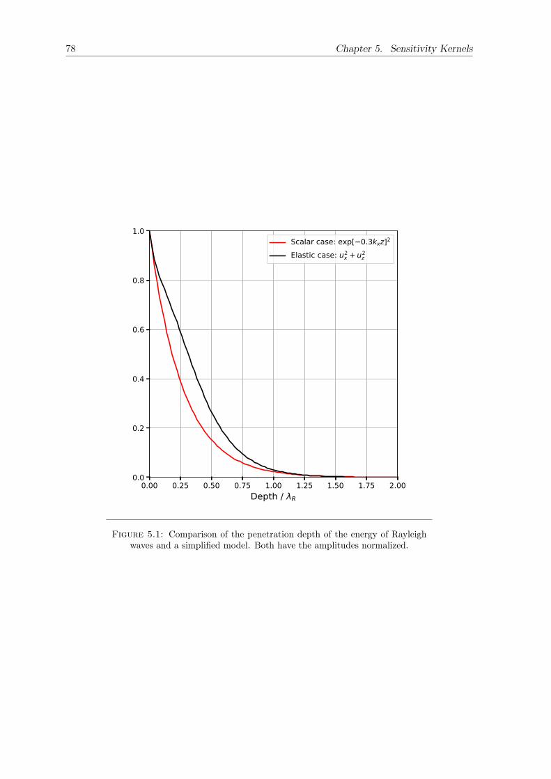
78 Chapter 5. Sensitivity Kernels
0.00 0.25 0.50 0.75 1.00 1.25 1.50 1.75 2.00Depth / R
0.0
0.2
0.4
0.6
0.8
1.0Scalar case: exp[ 0.3kxz]2
Elastic case: u2x + u2
z
Figure 5.1: Comparison of the penetration depth of the energy of Rayleighwaves and a simplified model. Both have the amplitudes normalized.

5.4. Phase velocity variation for surface waves 79
penetration with the elastic case, we can write Ls in terms of the Rayleigh wavelength usingthe proposed equivalence between both cases
Ls = 2α−1 = 2(0.3kR)−1 ≈ 1.06λR (5.19)
This result is coherent with the rule of thumb that estimates the penetration of theRayleigh waves around 1 horizontal wavelength λR.
5.4 Phase velocity variation for surface waves
The interaction of a surface wave with a perturbation in the medium is one the principalmechanisms that control the response that is recorded at the surface. This interaction isdifferent from that of the body waves in the sense that the surface waves propagate as awhole over a volume close to the surface, which implies that any small change in one layer ofthe medium within its penetration depth, should affect all the surface wave without breakingor changing its structure, which should remain the same for a given frequency. In particular,we are interested in determining how the surface phase velocity change with a fractional changein the bulk velocity. To do so, we begin with the Lagrangian that has the usual potential andkinetic terms of a wave scalar field, plus an elastic potential energy at the surface associatedwith the boundary condition:
L =1
2
[ρ(∂tu(t, r))2 − T (∇u(t, r))2 + αTu(t, r)2δ(z)
](5.20)
We integrate the Lagrangian over depth and average over one cycle to put it in terms ofthe energy integrals ∫ ∞
0〈L〉dz =
1
2
[ω2I1 − k2‖I2 − I3 + Is
](5.21)
where
I1 =1
2
∫ ∞0
ρh2dz, I2 =1
2
∫ ∞0
Th2dz,
I3 =1
2
∫ ∞0
T
(dh
dz
)2
dz, Is =1
2
∫ ∞0
αTh2δ(z)dz.
(5.22)
Now, following Aki and Richards (2002) we find the perturbation of this expression, thatis equal to
ω2δI1−k2‖δI2 − δI3 + δIs
= ω2
∫ ∞0
ρhδhdz − k2‖∫ ∞0
Thδhdz −∫ ∞0
Tdh
dz
dδh
dzdz +
∫ ∞0
αThδhδ(z)
=
∫ ∞0
ω2ρh− k2‖Th+
d
dz
(Tdh
dz
)δhdz − T
dh
dzδh
∣∣∣∣∞0
+ αThδh|z=0
(5.23)
The terms inside the curly brackets are equal to the application of the equation 5.1 to thesurface eigenfunction and therefore, equal to zero
− ρω2h+ Tk2‖h− Td2h
dz2= 0 (5.24)

80 Chapter 5. Sensitivity Kernels
The two remaining terms on the rigth hand side of equation 5.23 can be simplified knowingthat δh = 0 at z =∞ and using the boundary condition dh/dz|z=0 = −αh|z=0
Tdh
dzδh
∣∣∣∣z=0
+ αThδh|z=0 = T (−αh)δh|z=0 + αThδh|z=0 = 0 (5.25)
Therefore, the integrated Lagrangian is stationary for a perturbation of the surface eigen-function
ω2δI1 − k2‖δI2 − δI3 + δIs = 0 (5.26)
On the other hand, we can show that the integrated lagrangian 5.21 is equal to zero forthe surface eigenfunction as expected from the energy conservation. To do so we multiply5.24 by −h/2 and integrate it over depth to obtain
0 =1
2
∫ ∞0
ρω2h2dz − 1
2
∫ ∞0
Tk2‖h2dz +
1
2
∫ ∞0
Thd2h
dz2dz
=1
2
∫ ∞0
ρω2h2dz − 1
2
∫ ∞0
Tk2‖h2dz − 1
2
∫ ∞0
T
(dh
dz
)2
dz +1
2Th
dh
dz
∣∣∣∣∞0
(5.27)
The first three terms are I1, I2, and I3 respectively. Using the boundary conditions wecan write the last term as follows
− 1
2Th
dh
dz
∣∣∣∣0
= −1
2Th(−αh)|0 =
1
2
∫ ∞0
αTh2δ(z)dz = Is (5.28)
and thereforeω2I1 = k2‖I2 + I3 − Is (5.29)
Having established this, we proceed to find the change in the phase surface wave velocityas a consequence of a perturbation in the medium. To do so, we make a perturbation in theeigenfunction at fixed frequency h+ δh = h(ρ+ δρ, T + δT, k‖ + δk‖, ω), in the Lagrangian
ω2
∫ ∞0
(ρ+ δρ) (h+ δh)2 dz = (k‖ + δk‖)2
∫ ∞0
(T + δT ) (h+ δh)2 dz
+
∫ ∞0
(T + δT )
[d
dz(h+ δh)
]2dz −
∫ ∞0
α(T + δT ) (h+ δh)2 δ(z)dz
(5.30)
Eliminating perturbations of second order and subtracting the previous know relationsbetween the energy integrals, we obtain
∫ ∞0−2k‖δk‖Th
2 dz =
∫ ∞0
k2‖δTh2 dz +
∫ ∞0
δT
(dh
dz
)2
dz
−∫ ∞0
ω2δρh2 dz −∫ ∞0
αδTh2δz dz
(5.31)
From this we can calculate the change in phase velocity
(δcRcR
)ω
= −δk‖k‖
=
∫∞0
[k2‖h
2 +(dhdz
)2]δTdz −
∫∞0 ω2h2δρdz −
∫∞0 αδTh2δzdz
2k2‖∫∞0 Th2dz
(5.32)
5.5. Group velocity 81
We made a series of assumptions to simplify this expression: we assume that there is noperturbation of the density (δρ = 0) and that the background elastic constant T does notdepend on depth. We also suppose that the elastic constant is not perturbed at the surface(δT (z = 0) = 0) as a way to avoid perturbations over the boundary condition or over thesurface elastic energy that supports the surface waves. We then finally obtain(
δcRcR
)ω
=ρc2
2k2‖I2
∫ ∞0
[k2‖h
2 +
(dh
dz
)2]δc
c(z)dz (5.33)
where I2 is the energy integral defined in 5.22, and we made use of the relations betweenthe rigidity and the bulk velocity δT/T = 2δc/c, T = ρc2. This equation shows that anypossible variation of the bulk velocity will change the surface wave velocity as long as ithappens within the penetration depth determined by the surface eigenfunction. The weightof this integral will be written as
KCph(z) =ρc2
2k2‖I2
[k2‖h
2 +
(dh
dz
)2]
(5.34)
This expression shows us that the effective sensitivity reach of the surface waves at depthis proportional to the square of the eigenfunction and its derivative
5.5 Group velocity
The introduced frequency dependence of the parameter α used to trace a parallel with theelastic case, has a collateral effect over the group velocity of the surface waves. We recalcu-late this velocity with the variational approach previously introduced. First, we estimate aperturbation of the eigenfunction both in k‖ and in ω, h + δh = h(k‖ + δk‖, ω + δω), in theenergy integrals 5.29 to obtain
(ω + δω)2 (I1 + δI1) = (k‖ + δk‖)2 (I2 + δI2) + (I3 + δI3)− (Is + δI ′s) (5.35)
δI ′s can be calculated from the definition of I ′s (equation 5.22) keeping in mind that α isa frequency dependent quantity
δI ′s =1
2
∫ ∞0
αT2hδhδ(z)dz +1
2
∫ ∞0
δαTh2δ(z)dz = δIs +δα
αIs (5.36)
Subtracting equations 5.29 and 5.26 from this expression we find that
2ωδωI1 = 2k‖δk‖I2 −δα
αIs (5.37)
and therefore the group velocity is
U =δω
δk‖=k‖ω
I2I1− δα
δk‖
1
2αω
IsI1
(5.38)
We start evaluating some of these integrals. I2/I1 can be calculated from their definitions
I2I1
=T∫∞0 hδhdz
ρ∫∞0 hδhdz
= c2 (5.39)
On the other hand, from equation 5.6 α is
82 Chapter 5. Sensitivity Kernels
α =ω
c
√(c
cR
)2
− 1 (5.40)
Therefore
δα
δk‖= cR
δα
δω=cRc
√(c
cR
)2
− 1 =cRα
ω(5.41)
Finally, to evaluate Is and I1 we make direct use of the eigenfunction h = e−αz
I1 =1
2
∫ ∞0
ρh2dz =1
2ρ
(− 1
2αe−2αz
)∣∣∣∣∞0
=ρ
4α(5.42)
Is =1
2
∫ ∞0
αTh2δ(z)dz =1
2αT (5.43)
Putting all this together we obtain that
U =δω
δk‖=c2
cR− cR
α2
ω2c2 =
c2
cR− cR
(c2
c2R− 1
)= cR (5.44)
which conveniently fix the group velocity of surface waves with a lower value than thevelocity of body waves.
5.6 Time densities
Our objective is to determine how a fluctuation in the background velocity will affect theapparent velocity of the seismic field recorded at the surface. The two are related through thetypical time a seismic phonon passes in each part of a medium and the typical time it passeson each mode of propagation (in this case, as a body or as a surface wave). To analyze thiswe take a probabilistic approach. We begin denoting by A the event of the emission of theseismic phonon at time t0 = 0, B the event of a phonon propagating in time t′, and event Cthe phonon arriving at a receiver. The time will be implicitly included in the differentiationbetween events A, B, and C marking a temporal transition between them. The probability ofeach event will be written as P (E) where E represents the event. The state of each phononin one event is specified with a subindex marking its position r, its direction k, or its mode ofpropagation m; the mode is b or s when the phonon propagates as a body or surface particlerespectively. For example, P (Bz′,b′) is the probability that the phonon is propagating in timet′ as a body particle at depth z′, independently of its radial position r of the direction ofpropagation k. Therefore, P (Bb′) is the probability that the phonon was propagating in timet′ as a body particle, irrespective of its position or its direction. Naturally, P (Bb′) is the sumof P (Bz′,b′) for all the depths, which for a continuous system can be written as
P (Bb′) =
∫z′P (Bz′,b′)dz
′ (5.45)
In general, removing an index of an event probability implies grouping all the eventsdesigned by that index by summing their individual probabilities
P (Ei,j) =∑k
P (Ei,j,k) (5.46)

5.6. Time densities 83
We can divide specify the event set with any index classification we want as long as itcovers the original set completely, or in other words, under the condition that it forms asample space of the original event (Miller and Childers, 2012).
The probability that a phonon arrives to the receiver at r under the condition that it wasemitted at the source in r0, can be written as the conditional probability P (Cr | Ar0) (Gut,2013). We can rewrite this in terms of conditional probabilities with an intermediate stateof propagation using the Chapman–Kolmogorov equation (Ross, 2014; Papoulis and Pillai,2002; Roepstorff, 2012)
P (Cr | Ar0) =
∫ωP (Cr | Bω)P (Bω | Ar0) dω (5.47)
where ω represents every single outcome of the probability sample space. This equationsays that the probability of going from event A to C can be found from the probabilities of thephonon going from A to B and from B to C, as long as we add all the possible intermediateevents B. The sample space can be classified in different ways: for example, we could specifythe event B uniquely for its position, and this would effectively cover the whole range ofpossibilities.
P (Cr | Ar0) =
∫r′P (Cr | Br′)P (Br′ | Ar0) dr′ (5.48)
However, this election would only allow us to describe a system on which the propagationdirection of each of the phonons is independent of its position: this is the case of a diffusivesystem as was proposed by Pacheco and Snieder (2005). If we want to describe the first stagesof the system this description is inadequate as they are marked by a strong directionality ofthe propagation of the waves (Margerin et al., 2016). Therefore, we classify the sample spacewith a combination of the position, the direction, and the mode of propagation of each phonon
P (Cr | Ar0) =
∫r′
∫k′
∑m
P (Cr | Br′,k′,m)P (Br′,k′,m | Ar0) dk′ dr′ (5.49)
k′ was not specified in the source or the arrival events because the direction of propagationof the phonons at those events is not important. Notice that the integration of equation 5.49over all directions (and modes) does no lead to equation 5.48 because it implies a joint inte-gration between the two conditional probabilities sharing the same k′. Integrating equation5.49 over the time of the propagation event B (t′) for all the possible travel times (between 0and t), and reorganizing the terms gives
t =
∫r′
[∫ t
0
∫k′
∑m
P (Cr | Br′,k′,m)P (Br′,k′,m | Ar0)
P (Cr | Ar0)dk′dt′
]dr′ (5.50)
The parenthesis was added to highlight the fact that the term inside is the time sensitivitykernel (Pacheco and Snieder, 2005; Margerin et al., 2016), extended to track the two possiblemodes of propagation. To simplify this equation and to approach us to the measurementsmade in the Monte Carlo simulation, we assume that we’re only interested in the phononsemitted by the source at the location r′ = 0 (source in the surface), which forms now ourwhole and only set of particles. This allows us to drop the references to the event A
t =
∫ t
0
∫r′
∫k′
∑m
P (Cr | Br′,k′,m)P (Br′,k′,m)
P (Cr)dk′dr′dt′ (5.51)
Using the Bayes formula (Papoulis and Pillai, 2002; Gut, 2013)

84 Chapter 5. Sensitivity Kernels
P (Cr | Br′,k′,m)P (Br′,k′,m) = P (Br′,k′,m | Cr)P (Cr) (5.52)
we can rewrite equation 5.51 as
t =
∫ t
0
∫r′
∫k′
∑m
P (Br′,k′,m | Cr) dk′dr′dt′ (5.53)
Thanks to the simplification made, we can now integrate over all directions
t =
∫ t
0
∫r′
∑m
P (Br′,m | Cr) dr′dt′ (5.54)
Now, we proceed to make explicit the contribution of each mode, and to simplify the spatialdependence integrating over the whole space for the surface mode, and over the horizontalplane for the body mode
t =
∫ t
0P (Bs′ | Cr) dt
′ +∫ t
0
∫z′P (Bz′,b′ | Cr) dz
′dt′ (5.55)
The surface mode of propagation does not depend on the depth and for that reason, itsprobability was fully integrated. Before going any further, it is useful to interpret each of theseprobabilities as a counting process. Let us imagine that we shoot a great number of seismicphonons from the source, some of which reach the receiver at time t; if we receive a numberhigh enough of particles, their travel histories will be representative of all the possible pathsto go from the source to the receiver. This is the set of particles that fulfill the condition ineach of the conditional probabilities of equation 5.55: arrive to the receiver located at r in thetime t. Because they represent the whole set of possibilities, estimating one probability canbe done by counting: for example, if we want P (Bz′,b′ | Cr), we just have to count the numberof body wave particles that were at the position z′ in the time t′ and divide this number bythe total of particles that arrive to the receiver. Therefore, equation 5.55 can be written as
t =
∫ t
0
Ns(t′)
Ndt′ +
∫ t
0
∫z′
Nb(z′, t′)N
dz′dt′ (5.56)
The relationship stated here will be fundamental later on: integrate the probability thata particle propagates in a certain mode between all the possible travel-times is equivalent tosum the time spent by all the particles in that mode and divide it by the total number ofparticles, or in other words, is equivalent to the average time spent in that mode∫ t
0P (Bm′ | Cr) dt
′ =∫ t
0
Nm(t′)N
dt′ = tm (5.57)
On these terms, equation 5.55 can be written as
t = ts +
∫z′tb dz
′ (5.58)
which makes evident that their sum is equal to the total lapse time. However, beforeproceeding with this change, let us come back to the probability description of the systemin equation 5.55: up until this point, the mode on which the seismic phonon arrives to thereceiver has been ignored. However, it can be made explicit adding the probabilities at thearrival point
5.6. Time densities 85
t =P (Cr,s)
P (Cr)
∫ t
0P (Bs′ | Cr,s) dt
′ +P (Cr,b)
P (Cr)
∫ t
0P (Bs′ | Cr,b) dt
′
+P (Cr,s)
P (Cr)
∫ t
0
∫z′P (Bz′,b′ | Cr,s) dz
′dt′ +P (Cr,b)
P (Cr)
∫ t
0
∫z′P (Bz′,b′ | Cr,b) dz
′dt′(5.59)
being P (Cr,m) the probability of the phonon arriving at time t and in mode m, to thereceiver located at (r, z). Before, the surface mode was not sub-classified at different depthsbecause it propagates as a whole in a parallel direction to the surface. However, at the arrivalpoint it becomes necessary as the energy of the surface waves is highly dependent on thedepth and therefore, the position of the receiver will determine how strong it is detected.The quantities in the form P (Cr,m)/P (Cr) can be interpreted as the fraction of particles thatarrive in a given mode m with respect to the total of particles that arrive to the receiver; giventhat each of these phonons represents a package of energy following the propagation schemedescribed by the transfer equations 5.14, this fractions can be written as Em(t, r)/E(t, r),being Em(t, r) the energy that arrives in the mode m to the receiver, and E(t, r) the totalenergy arriving at the same point. Using this equivalence and integrating for all the possibletravel times t′ results in
t =Es(t, r, z)
E(t, r, z)ts→s(t, r, z) +
Eb(t, r, z)
E(t, r, z)ts→b(t, r, z)
+Es(t, r, z)
E(t, r, z)
∫ ∞0
tb→s(z′; t, r, z) dz′ +
Eb(t, r, z)
E(t, r, z)
∫ ∞0
tb→b(z′; t, r, z) dz′
(5.60)
The semicolon in the arguments of each average time separates the variables of the propa-gation, from the variables of the arrival, and the subindex indicates the temporal sequence ofpropagation and arrival: for example, ts→b is the average time that the particles that arrivedin body wave mode, passed in surface wave mode. These times are schematized in figure 5.2for two simplified cases. Also, the position of the receiver r was explicitly put in terms of thedepth and the radial distance, profiting from the cylindrical symmetry of the system. Thisequation shows the flight distribution of the particles according to their mode of propagation,and the depth (in the case of body waves) at which they propagate. Notice that how theterms denominated by t in this equation are dimensionally different between them: for thepropagation of body particles we have times per unit of depth (tb→s and tb→b) and for thesurface waves they are simply times (ts→s and ts→b). Equation 5.60 describes what parts ofthe medium and what modes of propagation are the preferred for the particles traveling fromthe source to the receiver: a spatial and modal "distribution" of the total travel time. We cansimplify this equation by defining the effective time spent in each mode as an energy-weightedaverage between the two possible modes of arrival
〈ts(t, r, z)〉 =Es(t, r, z)
E(t, r, z)ts→s(t, r, z) +
Eb(t, r, z)
E(t, r, z)ts→b(t, r, z)
〈tb(z′; t, r, z)〉 =Es(t, r, z)
E(t, r, z)tb→s(z
′; t, r, z) +Eb(t, r, z)
E(t, r, z)tb→b(z
′; t, r, z)
(5.61)
which will result in a simpler version of equation 5.60
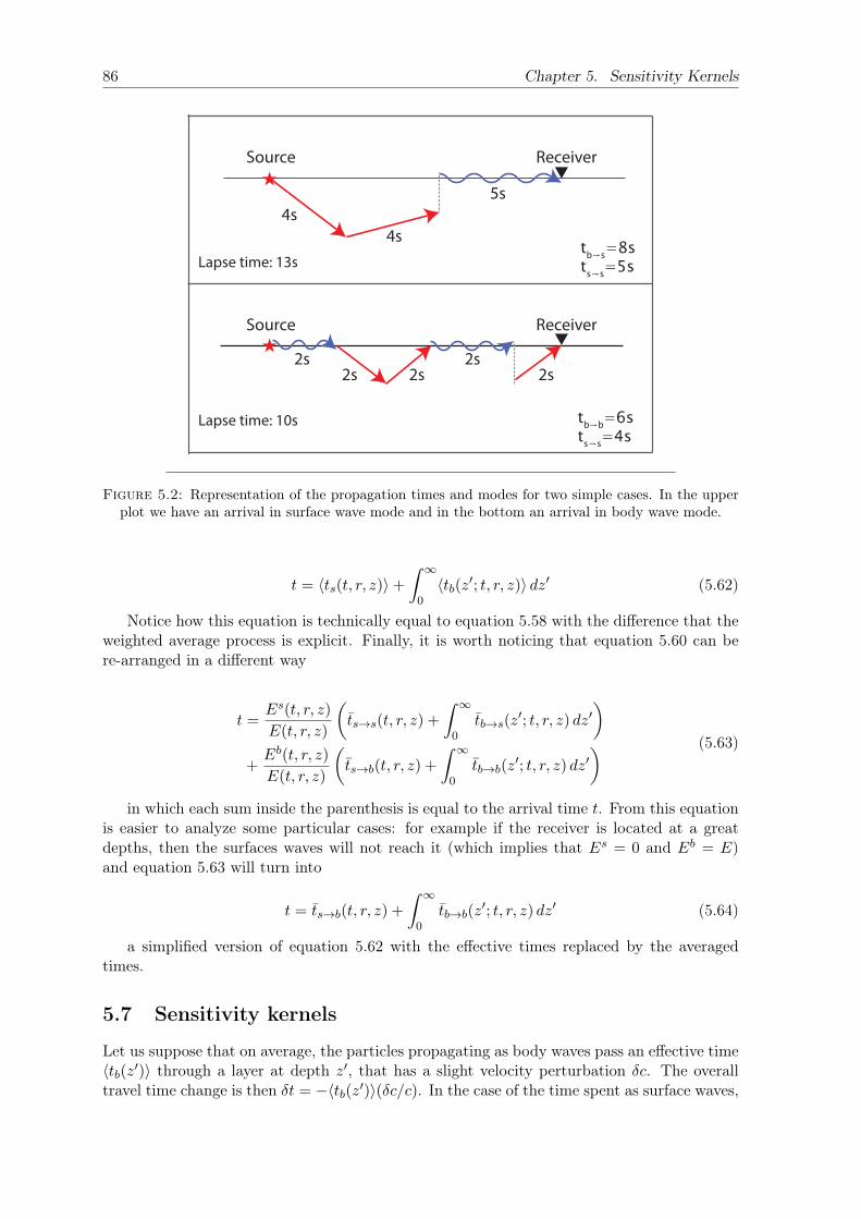
86 Chapter 5. Sensitivity Kernels
Source Receiver
Source Receiver
4s4s
5s
2s2s2s 2s 2s
Lapse time: 13s
Lapse time: 10s
tb→s=8sts→s=5s
tb→b=6sts→s=4s
Figure 5.2: Representation of the propagation times and modes for two simple cases. In the upperplot we have an arrival in surface wave mode and in the bottom an arrival in body wave mode.
t = 〈ts(t, r, z)〉+
∫ ∞0〈tb(z′; t, r, z)〉 dz′ (5.62)
Notice how this equation is technically equal to equation 5.58 with the difference that theweighted average process is explicit. Finally, it is worth noticing that equation 5.60 can bere-arranged in a different way
t =Es(t, r, z)
E(t, r, z)
(ts→s(t, r, z) +
∫ ∞0
tb→s(z′; t, r, z) dz′
)+Eb(t, r, z)
E(t, r, z)
(ts→b(t, r, z) +
∫ ∞0
tb→b(z′; t, r, z) dz′
) (5.63)
in which each sum inside the parenthesis is equal to the arrival time t. From this equationis easier to analyze some particular cases: for example if the receiver is located at a greatdepths, then the surfaces waves will not reach it (which implies that Es = 0 and Eb = E)and equation 5.63 will turn into
t = ts→b(t, r, z) +
∫ ∞0
tb→b(z′; t, r, z) dz′ (5.64)
a simplified version of equation 5.62 with the effective times replaced by the averagedtimes.
5.7 Sensitivity kernels
Let us suppose that on average, the particles propagating as body waves pass an effective time〈tb(z′)〉 through a layer at depth z′, that has a slight velocity perturbation δc. The overalltravel time change is then δt = −〈tb(z′)〉(δc/c). In the case of the time spent as surface waves,

5.8. Monte Carlo simulations 87
the travel time perturbation will have an analogous expression using the relative surface wavevelocity perturbation δt = −〈ts〉(δcR/cR). Therefore, the effective travel time delay generatedby any set of perturbations in the medium can be written as
δt = −〈ts(t, r, z)〉δcRcR−∫ ∞0〈tb(z′; t, r, z)〉
δc
c(z′)dz′ (5.65)
Putting the relative surface phase velocity perturbation in terms of δc at layer at depth z′
with equation 5.33, allow us to calculate the apparent velocity variation (δt/t = −ε) in termsof the bulk velocity variation
δt
t(t, r, z) =
∫ (−〈ts(t, r, z)〉
tKCph(z′)− 〈tb(z
′; t, r, z)〉t
)δc
c(z′)dz′ (5.66)
The term between parenthesis is the sensitivity kernel K; the left part is the surface wavesensitivity Ks and the right one the body wave sensitivity Kb. The negative signs indicatethat an increase of the velocity in the medium (δc/c > 0) generates an early phase arrival(δt/t < 0). Replacing the effective times by their definitions (equation 5.61) give us
δt
t(t, r, z) = −
∫ (Es(t, r, z)
E(t, r, z)Ks→s(z′; t, r, z) +
Eb(t, r, z)
E(t, r, z)Ks→b(z
′; t, r, z)
+Es(t, r, z)
E(t, r, z)Kb→s(z
′; t, r, z) +Eb(t, r, z)
E(t, r, z)Kb→b(z
′; t, r, z))δc
c(z′) dz′
(5.67)
where
Ks→s(z′; t, r, z) =ts→s(t, r, z)
tKCph(z′)
Ks→b(z′; t, r, z) =
ts→b(t, r, z)t
KCph(z′)
Kb→s(z′; t, r, z) =
tb→s(z′; t, r, z)t
Kb→b(z′; t, r, z) =
tb→b(z′; t, r, z)t
(5.68)
These equations show the contribution of each mode to the sensitivity and the depthdependence on the energy density of surface and body waves.
5.8 Monte Carlo simulations
The use of Monte Carlo simulations to recreate properties of the propagation of seismic wavesbegan with the application in equivalent acoustic systems that showed to be successful repro-ducing features like coda envelopes generated by earthquakes, or the study of the attenuationin different scattering regimes (Gusev and Abubakirov, 1987; Hoshiba, 1991; Abubakirov andGusev, 1990). This was later extended to models that include depth dependence of the ve-locity structure and the mean free path (Hoshiba, 1997; Margerin, Campillo, and Tiggelen,1998), elastic propagation modes (Margerin, Campillo, and Van Tiggelen, 2000; Przybilla,Korn, and Wegler, 2006), lateral heterogeneous scattering and non-isotropic scattering (Sens–Schönfelder, Margerin, and Campillo, 2009), or coupling between surface and body scalar

88 Chapter 5. Sensitivity Kernels
Surface
Receiver volume
Figure 5.3: Model of the Monte Carlo simulations. The red star marks the location of the source,and the grey volume represents the receiver zone.
waves (Margerin, Bajaras, and Campillo, 2019). Here, the last case will be further exploredtowards the estimation of the time sensitivity kernels of both body and surface waves
5.8.1 General outline
The objective of the Monte Carlo simulations is to recreate the conditions set by the energytransport equations shown in 5.14, and to make measurements of the time spent at eachdepth and mode in a layered system. The general procedure consists in shooting many seismicparticles from the source, and allow them to travel in a straight line until they are scattered;after each of these scattering events, a new direction and mode are chosen randomly followingcertain probability distribution, and the particle continues its propagation. The time betweenscattering events is statistically controlled by the mean free time of each mode. The receiver isdefined as a small finite volume through which the particles must cross in order to contributeto the energy density and to the sensitivity measured from that point, at that particular time.This is the particle counting method (Sens–Schönfelder, Margerin, and Campillo, 2009; Gusevand Abubakirov, 1987). One of the main disadvantages of this method is that the probabilitythat a particle doing a random walk will pass through the receiver at a given time is low;this is partially compensated by shooting many particles from the source, and exploitingthe symmetries of the system which may allow to turn the receiver into bigger volume. Forexample, if we have a completely symmetric full-space, the receiver can be turned into aspherical shell. In our case, the half-space symmetry allows us to have a ring-shaped receiveraround the source. it is worth noticing however that this symmetry can be broken if thesources are non-isotropic, although this is not our case. The geometry used here if illustratedin figure 5.3.
Nonetheless, maybe the main advantage of this method is that it allows us to follow thetrajectories of all the phonons and measure the time that each of them passes on every partof the medium and on every mode. With these measurements, we can calculate the timedensities for each mode and depth that are the basis of the sensitivity kernel as was explainedin the previous sections. Next, we present the most important aspects of the simulations
5.8. Monte Carlo simulations 89
Propagation: A big number of particles are shot from a source located at the surface inrandom directions, with initial modes chosen probabilistically to follow equations 5.15.The body mode propagates in three dimensions and the surface mode in two; this meansthat the surface particles do not have any depth coordinate. Each particle propagatesin a straight line in a random isotropic direction assigned at the beginning. The timeof propagation or free time of flight is also chosen randomly in such a way that itsdistribution reconstructs the exponential probability density function τ−1et/τ (Welch,Van Gemert, and Others, 2011) where τ is the mean free time. This means free timeis chosen according to the mode and depth of the particle (for the case of the bodyparticles) as indicated in equation 5.9. For the case of body waves, the dependenceof the mean free time on the depth is simplified through the method of delta collisionswhich introduce virtual scattering events that do not modify the direction of propagation(Lux, 2018). If a body particle reaches the surface, its movement is completely reflectedinto the half-space without modifying any other parameter.
Scattering: Once the simulation time reaches the the free time of flight, a scattering eventoccurs. A new propagation direction and mode are chosen. The mode is chosen ran-domly between the two possible outcomes using their respective mean free times asweights for each option. For example, the probability that a body wave scatter into asurface wave is
pb→s(z) =(τ b→s(z))−1
(τ b→s(z))−1 + (τ b→b)−1(5.69)
It follows then that the probability that a body wave scatters into another body waveis pb→b = 1 − pb→s. Notice that for this particular case, when the body particle is faraway from the surface, the probability of changing into a surface particle is practicallyzero. When a surface particle scatters into a body particle, the depth of the particle isdefined randomly following the probability density function 2αe−2αz, which representsthe normalized energy density of the surface waves.
Time bookkeeping: In order to measure the time densities in equation 5.60, the half-spaceis virtually segmented in horizontal layers. When the particle is propagating as a bodywave, we keep track of the time spent in each of these layers; these times tb, are addedbetween them when the particle passes several times through the same layer. If theparticle propagates as a surface wave, the time is registered and accumulated as theindependent value ts. This process is illustrated in figure 5.4. it is important to re-member that although from the bookkeeping process the times recorded in a body orsurface modes seem equivalent, for the body waves case we are technically registeringthe time per unit of layer length, contrary to the case of the surface waves where we’reregistering directly the total time as was explained in the section 5.6.
Detection and averaging: The source and the receiver are both located in the same posi-tion over the surface to reproduce measurements of the seismic field obtained throughthe auto-correlation. However in the practice, the receiver is a cylindrical volume: if theparticle is inside it, then it is assumed that it arrived to the receiver. This is illustratedin figure 5.3. At the times at which we want to measure the sensitivity (the lapse times),the simulation evaluates if the particle is inside the receiver volume: if that’s the case,the bookkept times are registered along with the mode of the particle at that instant asthis is the arrival mode. If not, no registering process is performed but the simulation

90 Chapter 5. Sensitivity Kernels
ts
tb
0 0
0
3
6
3
Surface
12time between scatterings =
(a) The time spent by the body particle isrecorded independently for each layer
ts
tb
12 0
0
3
6
3
Surface
12time between scatterings =
(b) The time spent as a surface particle isrecorded independently
ts
tb
2
4
12 4
2
3
6
3
Surface
12time between scatterings =
(c) If the body particle reaches the surface, thetime is recorded temporarily beyond it
ts
tb
0
0
12 8
4
3
6
3
Surface
12time between scatterings =
(d) The times beyond the surface are summed tothe layers within the half-space
Figure 5.4: Time bookkeeping for body and surface waves. The probabilistic character of the timebetween scatterings events has been simplified.

5.9. Surface and body wave sensitivity 91
Variable Monte Carlofrequency* (Hz) 5.25α* (km−1) 2.86Surface penetration depth Ls (km) 0.7B. energy velocity cE (km/s) 3.9S. energy velocity cR (km/s) 3.7Mean free time τ b→b (s) 0.35Mean free path lb→b (km) 1.37Grid spacing gr (m) 50Receiver radius* (km) 5.7Receiver depth* (m) 20Model depth (km) 6Model radius* (km) 5.7
Table 5.1: Parameters used in the Monte Carlo simulations. The half-spacehas no bounds; the last two parameters are only relevant for the absorbingboundary conditions. The parameters with an asterisk may differ from Ober-mann et al. (2016) for reasons explained in the text; α is included in this list
as it has no equivalent in the elastic case.
Figure 5.5: Model used by (taken from) Obermann et al. (2016). The red star marks the sourcepositions and the inverted triangles the receiver positions
continues because it is still possible that the particle will be within the receiver volumefor another measurement at a later lapse time.
After all the particle paths have been simulated, the registered times are averagedbetween them for particles that arrived in the same mode to the receiver at a given timet, and that propagated at the same mode and at the same depth (for body waves). Thisprocedure gives us all the averaged times present in equation 5.60.
5.9 Surface and body wave sensitivity
We begin making a quick summary of the method used by Obermann et al. (2016) in anelastic 3-D half-space; the model used can be seen in figure 5.5 They first estimate the surfaceand body wave contributions to the apparent velocity variation independently. The surfacecontribution εSurf is determined with a series of simulations in a 3-D homogeneous half-space
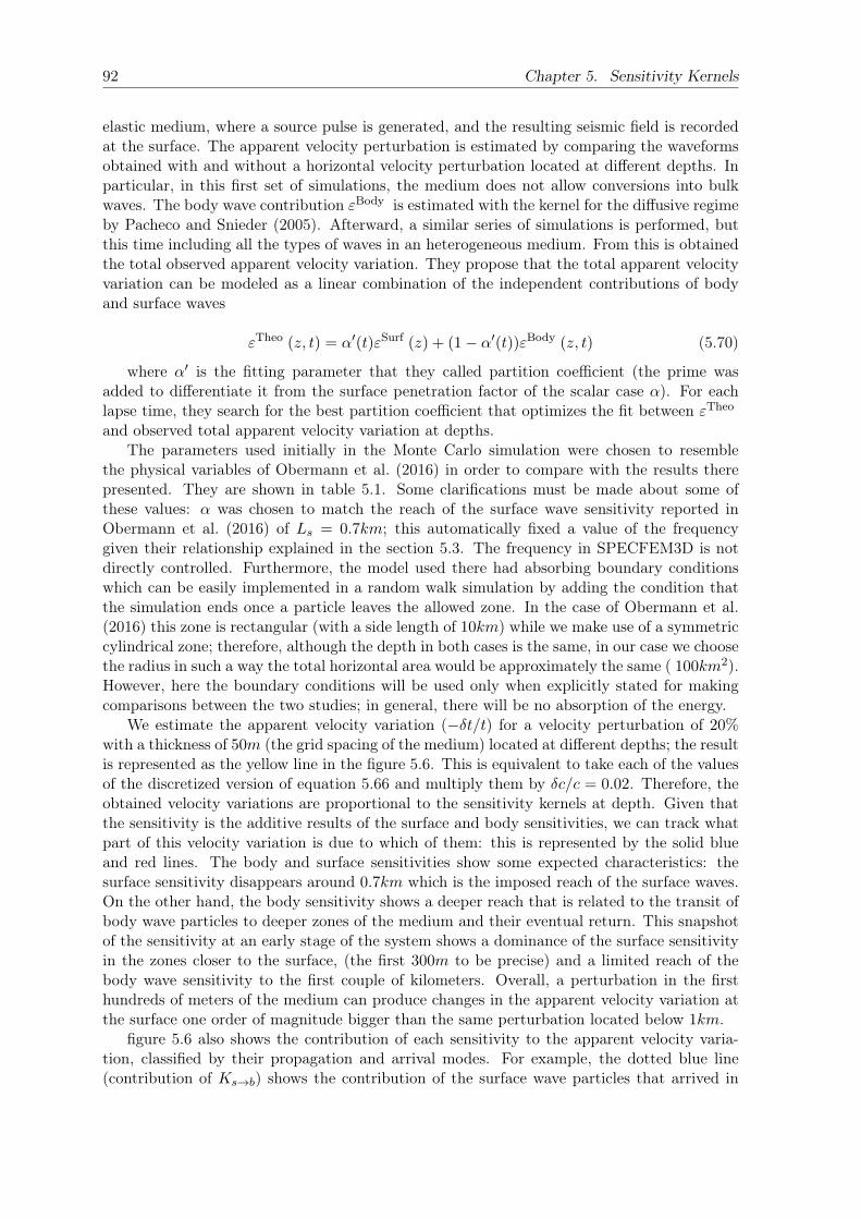
92 Chapter 5. Sensitivity Kernels
elastic medium, where a source pulse is generated, and the resulting seismic field is recordedat the surface. The apparent velocity perturbation is estimated by comparing the waveformsobtained with and without a horizontal velocity perturbation located at different depths. Inparticular, in this first set of simulations, the medium does not allow conversions into bulkwaves. The body wave contribution εBody is estimated with the kernel for the diffusive regimeby Pacheco and Snieder (2005). Afterward, a similar series of simulations is performed, butthis time including all the types of waves in an heterogeneous medium. From this is obtainedthe total observed apparent velocity variation. They propose that the total apparent velocityvariation can be modeled as a linear combination of the independent contributions of bodyand surface waves
εTheo (z, t) = α′(t)εSurf (z) + (1− α′(t))εBody (z, t) (5.70)
where α′ is the fitting parameter that they called partition coefficient (the prime wasadded to differentiate it from the surface penetration factor of the scalar case α). For eachlapse time, they search for the best partition coefficient that optimizes the fit between εTheo
and observed total apparent velocity variation at depths.The parameters used initially in the Monte Carlo simulation were chosen to resemble
the physical variables of Obermann et al. (2016) in order to compare with the results therepresented. They are shown in table 5.1. Some clarifications must be made about some ofthese values: α was chosen to match the reach of the surface wave sensitivity reported inObermann et al. (2016) of Ls = 0.7km; this automatically fixed a value of the frequencygiven their relationship explained in the section 5.3. The frequency in SPECFEM3D is notdirectly controlled. Furthermore, the model used there had absorbing boundary conditionswhich can be easily implemented in a random walk simulation by adding the condition thatthe simulation ends once a particle leaves the allowed zone. In the case of Obermann et al.(2016) this zone is rectangular (with a side length of 10km) while we make use of a symmetriccylindrical zone; therefore, although the depth in both cases is the same, in our case we choosethe radius in such a way the total horizontal area would be approximately the same ( 100km2).However, here the boundary conditions will be used only when explicitly stated for makingcomparisons between the two studies; in general, there will be no absorption of the energy.
We estimate the apparent velocity variation (−δt/t) for a velocity perturbation of 20%with a thickness of 50m (the grid spacing of the medium) located at different depths; the resultis represented as the yellow line in the figure 5.6. This is equivalent to take each of the valuesof the discretized version of equation 5.66 and multiply them by δc/c = 0.02. Therefore, theobtained velocity variations are proportional to the sensitivity kernels at depth. Given thatthe sensitivity is the additive results of the surface and body sensitivities, we can track whatpart of this velocity variation is due to which of them: this is represented by the solid blueand red lines. The body and surface sensitivities show some expected characteristics: thesurface sensitivity disappears around 0.7km which is the imposed reach of the surface waves.On the other hand, the body sensitivity shows a deeper reach that is related to the transit ofbody wave particles to deeper zones of the medium and their eventual return. This snapshotof the sensitivity at an early stage of the system shows a dominance of the surface sensitivityin the zones closer to the surface, (the first 300m to be precise) and a limited reach of thebody wave sensitivity to the first couple of kilometers. Overall, a perturbation in the firsthundreds of meters of the medium can produce changes in the apparent velocity variation atthe surface one order of magnitude bigger than the same perturbation located below 1km.
figure 5.6 also shows the contribution of each sensitivity to the apparent velocity varia-tion, classified by their propagation and arrival modes. For example, the dotted blue line(contribution of Ks→b) shows the contribution of the surface wave particles that arrived in

5.9. Surface and body wave sensitivity 93
0.0 0.2 0.4 0.6 0.8 1.0 1.2 1.4
Depth (km)
0.0
0.5
1.0
1.5
2.0
2.5
3.0
3.5
4.0
−δt/t
×10−3
Total apparent velocity variation
Contribution of surface waves
Contribution of body wavesContribution of Ks→sContribution of Ks→bContribution of Kb→sContribution of Kb→b
Figure 5.6: Total apparent velocity variation (yellow), associated to the body waves sensitivity (red),to the surface waves sensitivity (blue) and to each of the times densities in equations 5.67 and 5.68 at
a lapse time of 2s (normalized time of t/τ b→b = 5.7) with a velocity perturbation of δc/c = 0.02
body wave mode, and the dashed blue line (contribution of Ks→s) shows the contribution ofthe surface wave particles that arrived in the surface wave mode; the solid blue line is theweighted average between the two of them (as can be seen in equations 5.67 and 5.68). Thesensitivity on a given mode is always higher when the arrival happens in the same mode; forexample the contribution of Kb→b is higher than the contribution of Kb→s. At this lapse time(t/τ b→b = 5.7), there is still a low number of scattering events and therefore, a low probabilityof changing mode. However, the total surface and body wave sensitivities (the solid blue andred lines) seem the be closer to the surface mode arrivals (the dashed lines) indicating thatthe number of surface particles at the receiver is higher. This is related to the location ofthe receiver on the surface and is a common featured for all the results obtained with hisconfiguration.
The sensitivity at depth was obtained by Obermann et al. (2016) with a similar config-uration except for the presence of absorbing boundary conditions: it can be seen on the leftin figure 5.7. The yellow line represents the observed apparent velocity variation measured infull elastic simulations, the dashed black line is the result of the fitted model with equation5.70, and the dashed red line represents the estimation only due to the body sensitivity kernelcalculated from the equation of Pacheco and Snieder (2005). To compare with our case, weimposed also boundary conditions (the bounded geometry is indicated in the last two rows oftable 5.1 and recalculated the apparent velocity variation; the result is shown in the right offigure 5.7 (right panel). The resemblance between the two of them is remarkable, especially ifwe keep in mind that one of them is obtained in an elastic propagation field and the other ina scalar one. A quick comparison between this result and the one obtained without absorbingboundary conditions (figure 5.6) shows virtually no differences: although at this lapse time
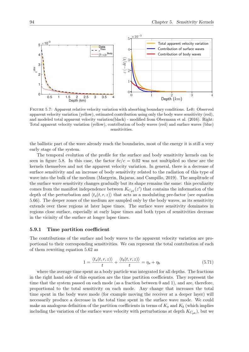
94 Chapter 5. Sensitivity Kernels
0 1 2 3 4Depth (km)
0
1
2
3
4
5
ε(−δt/t
)
×10−3
Total apparent velocity variation
Contribution of surface waves
Contribution of body waves
Figure 5.7: Apparent relative velocity variation with absorbing boundary conditions. Left: Observedapparent velocity variation (yellow), estimated contribution using only the body wave sensitivity (red),and modeled total apparent velocity variation(black) - modified from Obermann et al. (2016). Right:Total apparent velocity variation (yellow), contribution of body waves (red) and surface waves (blue)
sensitivities.
the ballistic part of the wave already reach the boundaries, most of the energy it is still a veryearly stage of the system.
The temporal evolution of the profile for the surface and body sensitivity kernels can beseen in figure 5.8. In this case, the factor δc/c = 0.02 was not multiplied so these are thekernels themselves and not the apparent velocity variation. In general, there is a decrease ofsurface sensitivity and an increase of body sensitivity related to the radiation of this type ofwave into the bulk of the medium (Margerin, Bajaras, and Campillo, 2019). The amplitude ofthe surface wave sensitivity changes gradually but its shape remains the same: this peculiaritycomes from the manifest independence between KCph(z′) that contains the information of thedepth of the perturbation and 〈ts(t, r, z)〉 that acts as a modulating pre-factor (see equation5.66). The deeper zones of the medium are sampled only by the body waves, as its sensitivityextends over these regions at later lapse times. The surface wave sensitivity dominates inregions close surface, especially at early lapse times and both types of sensitivities decreasein the vicinity of the surface at longer lapse times.
5.9.1 Time partition coefficient
The contributions of the surface and body waves to the apparent velocity variation are pro-portional to their corresponding sensitivities. We can represent the total contribution of eachof them rewriting equation 5.62 as
1 =〈ts(t, r, z)〉
t+〈tb(t, r, z)〉
t= ηs + ηb (5.71)
where the average time spent as a body particle was integrated for all depths. The fractionsin the right hand side of this equation are the time partition coefficients. They represent thetime that the system passed on each mode (as a fraction between 0 and 1), and are, therefore,proportional to the total sensitivity on each mode. Any change that increases the totaltime spent in the body wave mode (for example moving the receiver at a deeper layer) willnecessarily produce a decrease in the total time spent in the surface wave mode. We couldmake an analogous definition of the partition coefficients in terms of Ks and Kb (which impliesincluding the variation of the surface wave velocity with perturbations at depth KCph), but we

5.9. Surface and body wave sensitivity 95
0.00 0.25 0.50 0.75 1.00 1.25 1.50 1.75 2.00
Depth (km)
0
1
2
3
4
5
6
7
8S
ensi
tivi
ty(km−
1)
×10−2
Lapse time (s)
2.0
5.0
8.0
11.0
14.0
17.0
20.0
Body wave sens. Kb
Surface wave sens. Ks
Figure 5.8: Profile of the surface (dashed lines) and body (solid lines) waves sensitivity kernels atdepths, for different lapse times (indicated with colors)
will keep it in terms of the time densities as their interpretation is more immediate and it doesnot produce relevant changes in the result. We can extend this definition to the classificationby mode of propagation and arrival using the equation 5.63
1 =Es(t, r, z)
E(t, r, z)(ηs→s + ηb→s) +
Eb(t, r, z)
E(t, r, z)(ηs→b + ηb→b) (5.72)
where each sum inside the parenthesis is equal to 1. We can write the time partitioncoefficient for body and surface waves as a weighted average of these time partition coefficientsfollowing equations 5.61
ηs =Es(t, r, z)
E(t, r, z)ηs→s +
Eb(t, r, z)
E(t, r, z)ηs→b
ηb =Es(t, r, z)
E(t, r, z)ηb→s +
Eb(t, r, z)
E(t, r, z)ηb→b
(5.73)
The evolution of the partition coefficients in time can be seen in plot 5.9. At very earlylapse times, the time partition coefficient is strongly dominated by the surface waves becausethe location of the source favors the excitation of surface wave modes; this implies a predom-inance of the total surface wave sensitivity. The partition coefficients of body and surfacewaves are equal (the crossing point) around 6 mean free times: this marks the moment inwhich the body wave sensitivity starts dominating the total sensitivity.
figure 5.9 also shows the dynamics of the coefficients classified by modes of propagation andarrival. Just as before, the coefficients associated with the arrivals in the surface mode (the
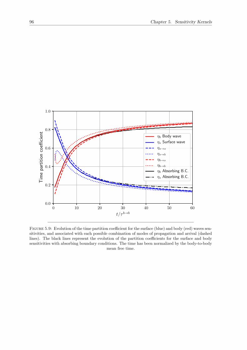
96 Chapter 5. Sensitivity Kernels
0 10 20 30 40 50 60
t/τ b→b
0.0
0.2
0.4
0.6
0.8
1.0
Tim
epa
rtit
ion
coeffi
cien
t
ηb Body wave
ηs Surface wave
ηs→sηs→bηb→sηb→bηb Absorbing B.C.
ηs Absorbing B.C.
Figure 5.9: Evolution of the time partition coefficient for the surface (blue) and body (red) waves sen-sitivities, and associated with each possible combination of modes of propagation and arrival (dashedlines). The black lines represent the evolution of the partition coefficients for the surface and bodysensitivities with absorbing boundary conditions. The time has been normalized by the body-to-body
mean free time.
5.10. Spatial scaling parameter 97
dashed blue ηs→s and red ηb→s lines) seem to be closer to the total average (the solid lines),especially at early lapse times. This indicates a bigger weight in the averages in equation5.73 as a consequence of a higher level of energy surface at the receiver. Let us focus onthe particles that arrive in the surface wave mode: the time partition ηb→s (red dashed line)is greater than ηs→s (blue dashed line) for long lapse times. Therefore, at this stage of thesystem, a surface particle arriving to the receiver has actually passed most of its travel timepropagating as a body particle. At this point, the difference of the time partition coefficientbetween the two arrival modes tends to disappear: for example, the difference between ηb→s(red dashed line) and ηb→b (red dotted line) is minimum at after 60 mean free times. Thisindicates that the system has spent a relatively large time in the diffusive state.
The application of absorbing boundary conditions (represented by the black lines) comesto be evident only after 30 mean free times, where we start seeing a decrease of the sensitivityof the body waves and an increase of the surface waves sensitivity. The absorption impliesremoving the paths between the source and the receiver that pass outside of the allowedvolume at any point. figure 5.10 shows the effect of the boundary conditions in the balancebetween the total surface and body waves energies for the whole space: as the surface particlescan only escape through the lateral side of the volume, while the body particles can do it bythe sides and the bottom, the rate of body phonons leaving the simulation is higher. It isthen clear that the surface sensitivity for the system with the absorbing boundary conditionsin figure 5.9 is higher because there is an over-representation of the paths that remain in thesurface wave mode of propagation. Although just a fraction of the phonons represented infigure 5.10 participate in the sensitivity and in the time partition coefficients measured inthe surface, for long lapse times the amount of energy sampling the medium is just a smallfraction of the total energy emitted by the source.
figure 5.11 shows a comparison of the evolution of the partition coefficient between theelastic case calculated by Obermann et al. (2016) (left) and the times partition coefficient inscalar case (right). In the elastic case, the time is normalized with the transport mean freetime, that is, the time over which a particle loses all information about the initial directionof propagation (Margerin, 2011; Sheng and Tiggelen, 2007). When the scattering is isotropic,as in our case, the transport mean free path and the mean free path are equal. Therefore, thetime in the Monte Carlo simulation is normalized with the body-to-body mean free time. Thesurface and body partition coefficients reach equal values (the crossing point) approximatelyat the same time for both cases; that this point is reached a bit later for the elastic case maybe related to the high surface sensitivity of the system at the beginning of the simulation incomparison with the scalar case. This is probably due to a strong excitation of surface wavemodes by the source whereas in our case this is statistically controlled to follow the energypartitioning ratio in the source radiation (equation 5.15). The other important differencecomes from the partitioning coefficient at long lapse times: the elastic case seems to showa strong tendency towards the disappearance of the surface sensitivity. In the scalar case,this process is more gradual as it shows a rate of energy transfer of surface wave energy intobody wave energy proportional to the squared root of time (Margerin, Bajaras, and Campillo,2019).
5.10 Spatial scaling parameter
The mean free time is a natural scaling factor for the time as it quantifies the degree ofscattering in the system. In a propagation medium without boundaries, two systems withdifferent mean free times, but at the same normalized time t/τ , will have similar distributionsof energy and sensitivities in a system spatially scaled with mean free path. However, the
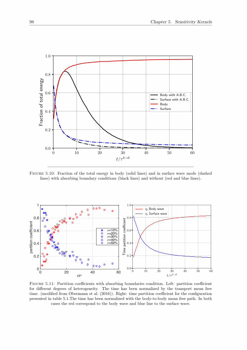
98 Chapter 5. Sensitivity Kernels
0 10 20 30 40 50 60
t/τ b→b
0.0
0.2
0.4
0.6
0.8
1.0
Fra
ctio
nof
tota
len
ergy
Body with A.B.C.
Surface with A.B.C.
Body
Surface
Figure 5.10: Fraction of the total energy in body (solid lines) and in surface wave mode (dashedlines) with absorbing boundary conditions (black lines) and without (red and blue lines).
0 10 20 30 40 50 60
t/τ b→b
0.0
0.2
0.4
0.6
0.8
1.0
Tim
epa
rtit
ion
coeffi
cien
t
ηb Body wave
ηs Surface wave
Figure 5.11: Partition coefficients with absorbing boundaries condition. Left: partition coefficientfor different degrees of heterogeneity. The time has been normalized by the transport mean freetime. (modified from Obermann et al. (2016)). Right: time partition coefficient for the configurationpresented in table 5.1.The time has been normalized with the body-to-body mean free path. In both
cases the red correspond to the body wave and blue line to the surface wave.
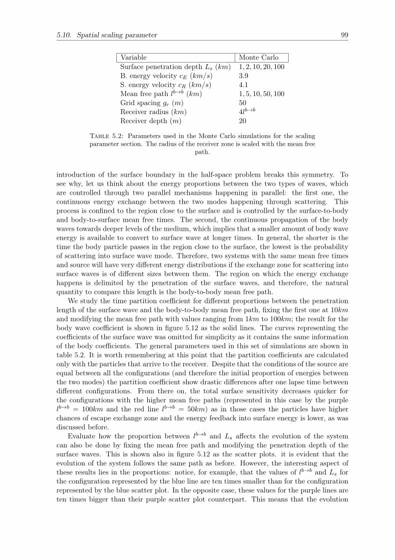
5.10. Spatial scaling parameter 99
Variable Monte CarloSurface penetration depth Ls (km) 1, 2, 10, 20, 100B. energy velocity cE (km/s) 3.9S. energy velocity cR (km/s) 4.1Mean free path lb→b (km) 1, 5, 10, 50, 100Grid spacing gr (m) 50Receiver radius (km) 4lb→b
Receiver depth (m) 20
Table 5.2: Parameters used in the Monte Carlo simulations for the scalingparameter section. The radius of the receiver zone is scaled with the mean free
path.
introduction of the surface boundary in the half-space problem breaks this symmetry. Tosee why, let us think about the energy proportions between the two types of waves, whichare controlled through two parallel mechanisms happening in parallel: the first one, thecontinuous energy exchange between the two modes happening through scattering. Thisprocess is confined to the region close to the surface and is controlled by the surface-to-bodyand body-to-surface mean free times. The second, the continuous propagation of the bodywaves towards deeper levels of the medium, which implies that a smaller amount of body waveenergy is available to convert to surface wave at longer times. In general, the shorter is thetime the body particle passes in the region close to the surface, the lowest is the probabilityof scattering into surface wave mode. Therefore, two systems with the same mean free timesand source will have very different energy distributions if the exchange zone for scattering intosurface waves is of different sizes between them. The region on which the energy exchangehappens is delimited by the penetration of the surface waves, and therefore, the naturalquantity to compare this length is the body-to-body mean free path.
We study the time partition coefficient for different proportions between the penetrationlength of the surface wave and the body-to-body mean free path, fixing the first one at 10kmand modifying the mean free path with values ranging from 1km to 100km; the result for thebody wave coefficient is shown in figure 5.12 as the solid lines. The curves representing thecoefficients of the surface wave was omitted for simplicity as it contains the same informationof the body coefficients. The general parameters used in this set of simulations are shown intable 5.2. It is worth remembering at this point that the partition coefficients are calculatedonly with the particles that arrive to the receiver. Despite that the conditions of the source areequal between all the configurations (and therefore the initial proportion of energies betweenthe two modes) the partition coefficient show drastic differences after one lapse time betweendifferent configurations. From there on, the total surface sensitivity decreases quicker forthe configurations with the higher mean free paths (represented in this case by the purplelb→b = 100km and the red line lb→b = 50km) as in those cases the particles have higherchances of escape exchange zone and the energy feedback into surface energy is lower, as wasdiscussed before.
Evaluate how the proportion between lb→b and Ls affects the evolution of the systemcan also be done by fixing the mean free path and modifying the penetration depth of thesurface waves. This is shown also in figure 5.12 as the scatter plots. it is evident that theevolution of the system follows the same path as before. However, the interesting aspect ofthese results lies in the proportions: notice, for example, that the values of lb→b and Ls forthe configuration represented by the blue line are ten times smaller than for the configurationrepresented by the blue scatter plot. In the opposite case, these values for the purple lines areten times bigger than their purple scatter plot counterpart. This means that the evolution

100 Chapter 5. Sensitivity Kernels
0 10 20 30 40 50 60
t/τ b→b
0.0
0.2
0.4
0.6
0.8
1.0
Tim
epa
rtit
ion
coeffi
cien
t
Ls = 10km
lb→b=1km
lb→b=5km
lb→b=10km
lb→b=50km
lb→b=100km
lb→b/Ls = 10
lb→b/Ls = 5
lb→b/Ls = 1 lb→b/Ls = 0.5
lb→b/Ls = 0.1
lb→b = 10kmLs=100km
Ls=20km
Ls=2km
Ls=1km
Figure 5.12: Body partition coefficient for different values of Ls and lb→b. Lines: time partitioncoefficient of body waves for a penetration length of Ls = 10km and different values of lb→b. Trianglescatter plots: time partition coefficient of body waves for a body-to-body mean free path of lb→b =10km and different values of Ls. The time has been normalized by the body-to-body mean free time.The dotted black line indicate the level at which the body and surface time partition coefficients are
equal (the crossing points)
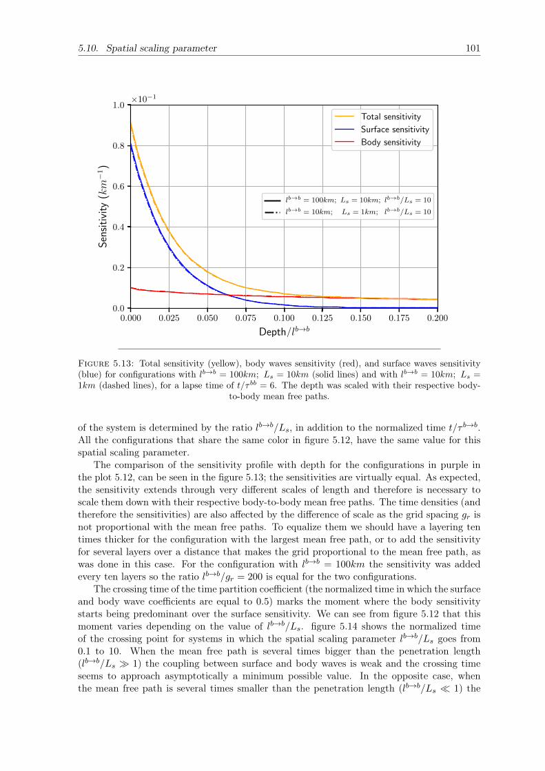
5.10. Spatial scaling parameter 101
0.000 0.025 0.050 0.075 0.100 0.125 0.150 0.175 0.200
Depth/lb→b
0.0
0.2
0.4
0.6
0.8
1.0S
ensi
tivi
ty(km−
1)
×10−1
Total sensitivity
Surface sensitivity
Body sensitivity
lb→b = 100km; Ls = 10km; lb→b/Ls = 10
lb→b = 10km; Ls = 1km; lb→b/Ls = 10
Figure 5.13: Total sensitivity (yellow), body waves sensitivity (red), and surface waves sensitivity(blue) for configurations with lb→b = 100km; Ls = 10km (solid lines) and with lb→b = 10km; Ls =1km (dashed lines), for a lapse time of t/τ bb = 6. The depth was scaled with their respective body-
to-body mean free paths.
of the system is determined by the ratio lb→b/Ls, in addition to the normalized time t/τ b→b.All the configurations that share the same color in figure 5.12, have the same value for thisspatial scaling parameter.
The comparison of the sensitivity profile with depth for the configurations in purple inthe plot 5.12, can be seen in the figure 5.13; the sensitivities are virtually equal. As expected,the sensitivity extends through very different scales of length and therefore is necessary toscale them down with their respective body-to-body mean free paths. The time densities (andtherefore the sensitivities) are also affected by the difference of scale as the grid spacing gr isnot proportional with the mean free paths. To equalize them we should have a layering tentimes thicker for the configuration with the largest mean free path, or to add the sensitivityfor several layers over a distance that makes the grid proportional to the mean free path, aswas done in this case. For the configuration with lb→b = 100km the sensitivity was addedevery ten layers so the ratio lb→b/gr = 200 is equal for the two configurations.
The crossing time of the time partition coefficient (the normalized time in which the surfaceand body wave coefficients are equal to 0.5) marks the moment where the body sensitivitystarts being predominant over the surface sensitivity. We can see from figure 5.12 that thismoment varies depending on the value of lb→b/Ls. figure 5.14 shows the normalized timeof the crossing point for systems in which the spatial scaling parameter lb→b/Ls goes from0.1 to 10. When the mean free path is several times bigger than the penetration length(lb→b/Ls 1) the coupling between surface and body waves is weak and the crossing timeseems to approach asymptotically a minimum possible value. In the opposite case, whenthe mean free path is several times smaller than the penetration length (lb→b/Ls 1) the
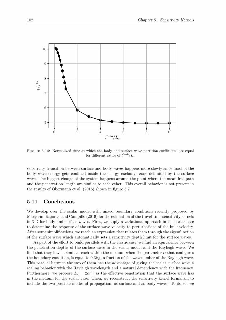
102 Chapter 5. Sensitivity Kernels
0 2 4 6 8 10
lb→b/Ls
5
6
7
8
9
10
t/τbb
Figure 5.14: Normalized time at which the body and surface wave partition coefficients are equalfor different ratios of lb→b/Ls
sensitivity transition between surface and body waves happens more slowly since most of thebody wave energy gets confined inside the energy exchange zone delimited by the surfacewave. The biggest change of the system happens around the point where the mean free pathand the penetration length are similar to each other. This overall behavior is not present inthe results of Obermann et al. (2016) shown in figure 5.7
5.11 Conclusions
We develop over the scalar model with mixed boundary conditions recently proposed byMargerin, Bajaras, and Campillo (2019) for the estimation of the travel-time sensitivity kernelsin 3-D for body and surface waves. First, we apply a variational approach in the scalar caseto determine the response of the surface wave velocity to perturbations of the bulk velocity.After some simplifications, we reach an expression that relates them through the eigenfunctionof the surface wave which automatically sets a sensitivity depth limit for the surface waves.
As part of the effort to build parallels with the elastic case, we find an equivalence betweenthe penetration depths of the surface wave in the scalar model and the Rayleigh wave. Wefind that they have a similar reach within the medium when the parameter α that configuresthe boundary condition, is equal to 0.3kR, a fraction of the wavenumber of the Rayleigh wave.This parallel between the two of them has the advantage of giving the scalar surface wave ascaling behavior with the Rayleigh wavelength and a natural dependency with the frequency.Furthermore, we propose Ls = 2α−1 as the effective penetration that the surface wave hasin the medium for the scalar case. Then, we reconstruct the sensitivity kernel formalism toinclude the two possible modes of propagation, as surface and as body waves. To do so, we

5.11. Conclusions 103
start with a classic probabilistic description of the transit of phonons from the source to thereceiver, which we extend towards different modes and depths. This includes also the modesof arrival to the receiver, and the corresponding equivalence to the energies ratios at thispoint. The conceptual link of each of these probabilities with the possible paths going fromthe source to the receiver is developed to establish a link with the time densities and with theMonte Carlo simulations to measure them. The formalism here presented has the advantagethat it can be easily extended to a full vectorial distribution of travel-time densities. Theseresults are used to construct an equation for the travel-time sensitivity kernel of the systemthat integrates the body and the surface wave sensitivities in a natural way.
A crucial part of the estimation of this kernel is the measurement of the time densities withthe Monte Carlo simulations which are described in detail. The initial set of parameters usedare chosen to mimic as close as possible the work of Obermann et al. (2016) where estimationsof the body and surface sensitivities were made with the help of full wavefield numericalsimulations. We evaluate the apparent velocity variation at the surface generated by a bulkvelocity perturbation located at different depths. As the kernel is a linear combination ofthe sensitivities of body and surface waves, the contribution of each of them to the apparentvelocity change can be estimated independently. The contribution of the surface waves islimited to an effective penetration equal to Ls as expected, while the body contribution is lessdominant at the surface but has a longer reach within the medium. The total sensitivity ofthe seismic field can be one order of magnitude stronger for perturbations close to the surface,than to perturbations located deeper in the medium.
The apparent velocity variation obtained by the scalar kernel with absorbing boundaryconditions holds a remarkable resemblance with the reported results by Obermann et al.(2016) both in amplitude and shape. The increase of lapse time in the system produces adecrease of the surface wave sensitivity that does not alter its shape but only its amplitude;this is a consequence of the independence between the depth and the temporal variables ofthe surface kernel. On the other hand, the body wave sensitivity increases its reach towardsdeeper levels of the medium. However, the sensitivity of both of them decreases progressivelyat the surface with time.
The time partition coefficients represent the total contribution of each of the modes ofpropagation to the total sensitivity of the system. The evolution of the coefficients charac-terizes the influence of one or other type of wave in the sampling of the perturbations atdepth in different moments of the system. At very short lapse times the surface waves dom-inate the sensitivity because the location of both the source and the receiver in the surfaceexcites predominately the surface wave modes. After, there is a decrease of the surface wavesensitivity coupled with an increase of the body wave sensitivity related to the progressivetransformation of surface wave energy into body energy and the continuous radiation of thislast one into the bulk of the medium (Margerin, Bajaras, and Campillo, 2019).
The inclusion of the absorbing boundary conditions is only evident after around 30 meanfree times, the point at which there seems to be a higher surface sensitivity (and lower bodysensitivity) with respect to the unbounded case. This can be explained in light of the energylosses generated by the absorption: although we observe a decrease in both types of energy,it is more accentuated for the body energy because the total area through which it canescape is bigger that for the surface case. This implies that the higher surface sensitivityin the absorbing case is just an artificial effect of the over-representation of the surface waveparticles in the calculation of the time densities. The comparison with the partition coefficientevolution obtained by Obermann et al. (2016) leads to similar crossing points but differs atlong lapse times where the scalar case tends to show a more gradual process of decrease(increase) of the surface (body) wave sensitivity.

104 Chapter 5. Sensitivity Kernels
The classification of the travel-time densities by their mode of propagation and arrival givesa deeper view into the dynamics of the system: there is a natural higher contribution of themode of arrival that coincides with the mode of propagation for both cases. This is a featurecharacteristic of an early stage of the system where the number of scattering events is stilllow, and therefore, there is a lower probability of changing mode arriving to the receiver thanto keep the same mode of propagation. At later stages we also see an equalization betweenthe partition coefficient for different arrival modes; this is a consequence of the system passingan increasing amount of time in a diffusive state on which there is no predominance of anymode on the arrival point beyond the one dictated by the modes density.
The evolution of a scattering system can be measured in terms of the normalized time.However, the introduction of the surface breaks this principle as the time that each bodyphonon passes in the exchange zone increases the probabilities of being scattered into a surfaceparticle, and therefore, affect drastically the overall energy balance between the two modes.The natural quantities that characterize this process are the body-to-body mean free pathand the thickness of the exchange zone, that is, the penetration of the surface wave. Weperform a series of simulations with different proportions between these two quantities thatshow that the evolution of time partition coefficient is highly dependent on them. When themean free path is considerably bigger than the penetration of the surface waves, the bodyand the surface waves are weakly coupled which implies that the body wave energy has morechances to radiate away from the exchange zone which accelerates the overall decrease ofthe surface wave sensitivity. In the opposite case, this process is more gradual as there isa continuous energy feedback between the two modes of propagation. We also observe aninvariance in the evolution of the time partition coefficient between systems that share thesame scaling parameter lb→b/Ls independently of the absolute values of lb→b and Ls. We showthat this invariance extends to their sensitivities profiles with depth as long as the distanceis normalized with their respective mean free paths lb→b, and the thickness of the grid usedto measure the time sensitivities is proportional to lb→b.
The crossing time (i.e. the moment on which the total body and surface wave sensitivitiesare equal to each other) marks the moment in which the body sensitivity starts dominatingin the system. An analysis of the dependence of this moment with the adimensional scaleof the system lb→b/Ls shows that the strongest qualitative change happens when this lastvalue is between 1 and 2; increasing this ratio decreases the coupling between the two modesand accelerates the domination of the body waves in the sensitivity. However, this processquickly reaches a minimum limit around 5 mean free times. On the other hand, decreasingthis ratio implies confining the body wave energy within the penetration zone of the surfacewaves, which generates a continuous feedback that delays the overtake of the body wave timepartition coefficient.
Despite the natural limitations of the scalar description of wave propagation (like thelack of polarization of the existence of a single mode of propagation for the body waves) ourapproach reproduces know features of the overall sensitivity in the system with the advantageof requiring low computational resources.

105
Chapter 6
Recovery of velocity variations atdepth
Andres Barajas, Ludovic Margerin, Michel CampilloArticle in preparation
Our objective now is to use the sensitivity kernels obtained in the preceding chapter tolocalize in depth the perturbations in the medium from a set of observations at the surface;this is the inversion problem. In this chapter we test the capabilities and limitations of thekernel to identify velocity variations in the crust under real-life conditions. In this sectionwe focus in the effect of three variables within the inversion: the depth of the perturbation,the duration of the coda segment to invert and the level of noise in the system. The resultshere presented are obtained for the autocorrelation configuration as the will be applied to thesingle-station measurements obtained in the chapter 3
6.1 Introduction
The seismic wavefronts propagating through the earth get distorted by the interaction withheterogeneities that scatter a fraction of their energy in different directions. This processproduces the characteristic coda wave segments after the main arrivals in the seismograms(Aki, 1969). Although complicated to analyze, the coda wave is not random and can beunderstood as the superposition of all the possible wave fronts that propagated through manydifferent paths when going from the source to the receiver (Snieder, 1999; Pacheco and Snieder,2005; Pacheco and Snieder, 2006). This implies that a complex seismogram generated by anseismic event can be reproduced if, by some mean, we repeat the same seismic source atthe same position; this has been observed with two of more earthquakes that occur in thesame location with very similar magnitudes (Geller and Mueller, 1980; Poupinet, Ellsworth,and Frechet, 1984; Beroza, Cole, and Ellsworth, 1995). However, although very similar, thereceived waveforms at the surface are not exactly equal: small variations are produced as aconsequence of small changes of the properties of the medium that happen in the period of timebetween the two seismic events. This is the main principle behind some studies that use thesealike earthquakes, called doublets, to track the changes in the velocity (Poupinet, Ellsworth,and Frechet, 1984; Ratdomopurbo and Poupinet, 1995) or in the attenuation (Beroza, Cole,and Ellsworth, 1995) of the crust.
The natural limitations of this approach are the scarce occurrence of doublets, and theimpossibility of applying this technique to zones where there is not strong seismic activity.This problem can be circumvented with Passive Image Interferometry (Sens-Schönfelder andWegler, 2006) which shows that the Green’s function of a random medium can be obtainedby cross-correlating the diffuse seismic fields registered by two receiver located in the surface

106 Chapter 6. Recovery of velocity variations at depth
(Campillo and Paul, 2003; Weaver and Lobkis, 2004). This means that a cross correlationbetween continuous recordings of noise at two stations is equal to what would be observedby one of the stations, if there were a unitary impulsive force at the other. The obtainedwaveforms have not only the ballistic part of the wave but also the coda, meaning that theseismic noise samples the medium in the same way a seismic event would do. The fluctuationof the phases in the coda of the cross correlations has allowed to estimate changes in thevelocity in the crust related to a variety of phenomena, like earthquakes (Brenguier et al.,2008a), volcanic activity (Rivet, Brenguier, and Cappa, 2015; Brenguier et al., 2008b), thethermoelastic response of the soil (Meier, Shapiro, and Brenguier, 2010), the earth tidesproduced by the sun and the moon (Sens-Schönfelder and Eulenfeld, 2019), among others.
The particular way in which the coda is perturbed is closely related to the lapse time thatthe wave had to travel from the source to the receiver, and the location of the perturbation inthe medium. Coda wave interferometry establishes the link between the perturbations of thewaveform at the receiver point and the location of the perturbation, through the introductionof the sensitivity kernels by Pacheco and Snieder (2005) and Pacheco and Snieder (2006).The sensitivity kernel is a travel-time density function that shows the most probable sectorsthrough which a wave would pass when going from the source to the receiver in a givenlapse time. The kernel can be calculated as a convolution of the probabilities of the particletraveling between the source, the receiver, and each part of the medium around them that issampled by the waves (Pacheco and Snieder, 2005; Margerin et al., 2016; Pacheco and Snieder,2003). Obermann et al. (2013a) and Obermann et al. (2016) proposed a sensitivity kernel forwave propagation in a 3-D half space as a linear combination of two independent sensitivities,one for surface and other for body waves, with a controlling factor mediating between themthat changes on time, and that is estimated through full wavefield numerical simulations. .This factor helps to recreate predominance of surface and body wave sensitivities at differentlapse times. In this work we use the sensitivity kernel described in the preceding chapter(based on the scalar model of Margerin, Bajaras, and Campillo (2019)) which estimates theprobabilities of propagation in surface and body modes with a series of Monte Carlo simulationthat integrates them simultaneously.
However, the process to obtain the parameters or sources, from the kernel and a series ofobservations is not straightforward: this is the inverse problem. The quality of the obtainedresults depends on the levels of noise in the system and on the specific conditions of themathematical function that relate the sources and the observations. For that reason it isimportant to know the capabilities and limitations of the kernel when applied to inversions.Towards that objective we perform a series of synthetic tests that are aimed at assessing thecapacity of the time sensitivity kernels to retrieve a velocity perturbation in different scenariosthat involve the depth of the perturbation in the medium, the set of measurements used, orthe level of noise in the system, for a setting where the source and the receiver are located inthe same position at the surface.
6.1.1 The inversion problem
Let’s imagine a system where we can define two physical quantities. When measured atdifferent positions or moments, these two quantities take a series of values that we can storein two vectors d and m, each of which have a number d and m of elements respectively. Let’ssuppose now that there is a causal relationship between the two variables: this means thatthe variation of the values in one of the variables m, that we will call the model, will generatechanges in the other variable d, that we will call the observations. This relationship betweenthem can be written as d = G(m), where G is a mathematical representation of the physicalmechanism that acts between the model and the observations, and that we will call generically

6.1. Introduction 107
the operator. If the relation between the model and the observations is linear, this relationcan be written simply as a matrix multiplication
d = Gm (6.1)
where G represents a d by m matrix. We assume that we can have access to the seriesof observations d, and that we can make a good mathematical representation of the physicalmechanism mediating between them, G. Then, the inversion problem consists in estimatingthe series of values of the model that generate the observations, or in other words, to obtainm. This problem can be seen as a minimization of the difference between the observed andthe calculated values of d, where the later is the multiplication between the operator and theestimation we make of the model
‖Gm− d‖ (6.2)
the accent in m highlights the fact that this is an estimated model. This minimizationproblem can be solved by the least-squares method, which provides us with the followingequation (Aster, Borchers, and Thurber, 2018; Snieder and Trampert, 1999)
m =(GTG
)−1GTd (6.3)
In an ideal case, the estimated and the real model parameters are equal m = m. One ofthe main difficulties related to the application of the inversion is the presence of noise whichmay produce unreliable or simply wrong estimations. The stability of the solution 6.3 to thenoise, lies in the intrinsic characteristics of the operator G; if the application of this formulaproduces the amplification of the noise (that is usually the case) the inverse problem is saidto be ill-conditioned.
Assessing the instability of the operator in the inversion can be done through its singularvalue decomposition (SVD), which allow us to write the d by m matrix G, as the product ofthree matrices:
G = USVT (6.4)
where U is a d by d orthogonal matrix whose columns U.,i span the data space, V is a mby m orthogonal matrix whose columns V.,i span the model space, and S is a d by m diagonalmatrix whose diagonal elements si are the so called singular values. It can be shown thatgiven the SVD, the estimated model m can written as (Aster, Borchers, and Thurber, 2018):
m =
p∑i=1
UT·,i · dsi
V·,i (6.5)
where p is the number of non-zero singular values. From this equation, it is clear thatthe solution is a linear superposition of the basis V.,i, with factors inversely proportional tothe singular values. If one of these singular values is unusually small in comparison with theothers, the introduction of a small amount of noise in the observations (d) will be amplified,and its associated term in the sum 6.4 will likely dominate the others. The condition numberof the operator is usually quantified by dividing the biggest singular value, that is also thefirst one, in the smallest one, that corresponds to the last one s1/sp; if this ratio is big, thenthe matrix G is probably ill-conditioned.
Qualitatively speaking, the problem is that the minimization of ‖Gm−d‖ may produce aresult that overfits m to the noise, generating estimations with big fluctuations, and therefore,unstable. This can be fixed if we try to minimize not only this quantity but also the norm of
108 Chapter 6. Recovery of velocity variations at depth
the solution itself ‖m‖. This ensures that the solution will be close enough to the observations,but at the same time that its amplitude will be controlled. The quantity to minimize will bethen
‖Gm− d‖2 + µ2‖m‖2 (6.6)
where µ is the regularization or damping parameter, in charge of controlling the trade-offbetween the minimization of the first and the second term. The least-squares approach forthis situation gives us the following solution
m =(GTG + µ2I
)−1GTd (6.7)
where I is a m by m identity matrix. The stabilization of the estimation through theintroduction of the new term can be seen explicitly if we write this equation in terms of thesingular value decomposition (Aster, Borchers, and Thurber, 2018)
m =
p∑i=1
s2is2i + µ2
UT·,i · dsi
V·,i (6.8)
where
fi =s2i
s2i + µ2(6.9)
are the filter factors. The introduction of the damping parameter helps to modulate thecontribution of the smallest singular values: if µ si the filter factor will be close to zerofi ≈ 0 and therefore there will be no contribution of the associated basis vector V.,i. On thecontrary, if µ si then fi ≈ 1 and the respective vector will contribute like in the no-dampedsolution. In this sense, the damping parameter works as a threshold value below which thesingular values, and their associated basis vector, are gradually excluded from the solution.Although this helps to control the influence of the noise, it inevitably reduces the precision ofthe estimated model, rendering it smoother and less complex.
In general, we search for a solution that can reproduce the observations with good preci-sion, without overfitting it to the presence of noise, or in other words, a solution with goodstability. The precision can be quantified through the the residual norm ‖Gm− d‖ and thestability through the norm of the solution itself ‖m‖; when performing inversions, we searchto balance the trade-off between them. In practice, different damping values minimize thesolution or the residual norm in such a way that plotting them simultaneously will give thecharacteristic trade-off L-curve that can be seen in figure 6.1; the dot marks the point thateffectively minimizes both parameters, although, in the practice, the best performing dampingparameter may not be necessarily exactly at this position, but close to it.
In the minimization problem can also be introduced a certain weight to each of the obser-vations or each of the parameters of the model, changing
m→ Lm d→ Qd (6.10)
This is a way to introduce information about the measurements uncertainties or aboutfeatures that we know (or want) our model should have (REF ASTER). Under these changes,the quantity to minimize is
‖Q(Gm− d)‖2 + µ2‖Lm‖2
= (Gm− d)TWd(Gm− d) + µ2mTWmm(6.11)
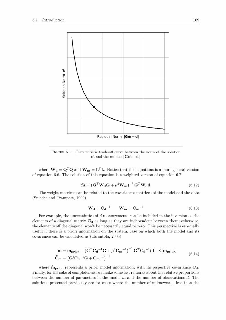
6.1. Introduction 109
Residual Norm |Gm d|
Solu
tion
Norm
m
Figure 6.1: Characteristic trade-off curve between the norm of the solutionm and the residue ‖Gm− d‖
where Wd = QTQ and Wm = LTL. Notice that this equations is a more general versionof equation 6.6. The solution of this equation is a weighted version of equation 6.7
m =(GTWdG + µ2Wm
)−1GTWdd (6.12)
The weight matrices can be related to the covariances matrices of the model and the data(Snieder and Trampert, 1999)
Wd = Cd−1 Wm = Cm
−1 (6.13)
For example, the uncertainties of d measurements can be included in the inversion as theelements of a diagonal matrix Cd as long as they are independent between them; otherwise,the elements off the diagonal won’t be necessarily equal to zero. This perspective is especiallyuseful if there is a priori information on the system, case on which both the model and itscovariance can be calculated as (Tarantola, 2005)
m = mprior +(GTCd
−1G + µ2Cm−1)−1GTCd
−1(d−Gmprior)
Cm =(GtCd
−1G + Cm−1)−1 (6.14)
where mprior represents a priori model information, with its respective covariance Cd.Finally, for the sake of completeness, we make some last remarks about the relative proportionsbetween the number of parameters in the model m and the number of observations d. Thesolutions presented previously are for cases where the number of unknowns is less than the
110 Chapter 6. Recovery of velocity variations at depth
number of observations (m > d), with exception of the equations in terms of the singularvalue decomposition, that are applicable for all the cases. When there are more unknownsthan observations (m > d) there are many possible solutions and the optimization criteria isthe minimization of ‖m‖ which leads to slightly different versions of the equations 6.3, 6.7 and6.12 . However, most of the cases of interest for us are over-determined, mixed-determined,or weakly under-determined and for all of these cases, the best approach is the one thatwas presented here. The interested reader can find an extensive discussion about both theover-determined and the under-determined problem and its solutions in Menke (2018).
6.2 Setting of the seismic inverse problem
If we compare two seismograms obtained before and after the inclusion of a small velocityperturbation in a heterogeneous medium, we would notice a small phase shift between them(Obermann et al., 2013a). These phase perturbations can be interpreted as an apparentvelocity variation of the seismic field (ε = −δt/t). Our objective is to deduce the variations ofvelocity generated in the crust from the measured apparent velocity variations at the surface.Therefore, the changes in velocity at depth are the components of the model vector
m =
(δc
c(z1),
δc
c(z2), · · · ,
δc
c(zm)
)(6.15)
and the apparent velocities measured at the receptor at different lapse times are thecomponents of the vector of observations
d = (ε(t1), ε(t2), · · · , ε(td)) (6.16)
For most of practical applications, the coda wave of the seismograms is retrieve withseismic interferometry, which is obtaining the medium’s Green’s function from the cross-correlation of continuous records of the ambient seismic noise in the surface (Weaver andLobkis, 2004; Campillo and Paul, 2003). Each segment of the coda of these correlations isrepresentative of a part of the energy that traveled from the source to the receiver. Then, intheory, measuring this phase delay for every point in a long enough coda would give us asmany measures as we want which would be advantageous to perform the inversion. However,in practice, the obtained correlations are far from perfect due to factors like unstable or non-symmetric noise sources (Snieder, 2004; Liu and Ben-Zion, 2013). Even with ideal noise-freecorrelations, it is desirable to limit the observations of the apparent velocity variations to acertain frequency range which implies dividing the coda in windows wide enough to containseveral oscillations of the desired frequencies. This means that every estimation of δt/t is notmade with a very specific lapse time but with a portion of the coda around it. The limitationsare also related to the overall portion of the coda that can be used to measure the phase delay:at later lapse times there is a natural decrease of signal-to-noise ratio so the measurementsbecome unreliable. All these factors limit the useful portion of the coda to make the inversion,and the number of measurements we can take from it.
6.2.1 Construction of the operator G
The relation between the apparent velocity measurements in the surface and the velocityvariations at depth can be represented as
6.2. Setting of the seismic inverse problem 111
d = G mε(t1)ε(t2)...
ε(td)
=
G1,1 G1,2 · · · G1,m
G2,1 G2,2...
. . .Gd,1 Gd,m
(δc/c)(z1)(δc/c)(z2)
...(δc/c)(zm)
(6.17)
The operator G can be constructed with the sensitivity kernel obtained previously in 5.66,but adapted to a discretized medium
G = (Gi,j) =
(〈ts(ti)〉ti
KCph(zj) +〈tb(zj ; ti)〉
ti
)(6.18)
where the source and the receiver were assumed to be at the same place in the surface(z = 0, r = 0). Each row of the operator is related to the travel-time of the phonons goingfrom the source to the receiver ti, and each column to the depth through which they passedduring this process at any time zj ; this is the reason why a colon has been preserved in thenotation of tb(zj ; ti), making a clear distinction between the variables that refer to the transitof the phonon through the medium, and the variables that make reference to the arrival event.From this equation is clear that the dimensions of the operator are dependent of the amountof observations made d, and on the desired layers to resolve through the inversion m. Thefirst term of the right hand side of the equation 6.18 is representative of the surface wavessensitivity, and the second one of the body waves sensitivity.
The quantities ts(ti) and tb(zj ; ti) are estimated through the Monte Carlo simulation aswas explained in the preceding chapter. For a chosen set of parameters, a single simulation isrun registering ts and tb, in many different lapse times ti, with a very high depth resolutionwhich is obtained dividing the half space in many thin layers zj . The operator G formedwith all the registered lapse times over a set of very thin layers, will be referred to as thehigh-resolution operator. However, real applications of the inversion will be done over a moresparse set of lapse times (equal to the measurements of δt/t), to obtain velocity perturbationsin a relatively thick layered system (with every layer in the order of kilometers or hundredsof meters). The full-resolution operator can be adapted for these applications as follows:
Time axis: The closest lapse time of the simulation is chosen, and its respective row in the operatoris preserve, meaning that all the others are simply removed. This decrease the numberof rows of the operator to the same number of measurements of the apparent velocityvariation or δt/t.
Depth axis: The sensitivity between different columns is grouped and summed to match the desiredthickness. For example, from an operator layered every 0.2km, can be constructed anew operator layered every 1km, summing every 5 columns of the operator.
After this procedure the resulting operator will have less columns than the full-resolutionoriginal operator. We will refer to the operator with both axis reduced, as the down-sampledoperator Gds .
6.2.2 Parameters election
With the purpose of obtaining velocity perturbations in the crust from real data obtained inthe region of Pollino, in the south of Italy, the parameters of the construction of the kernelwere chosen to resemble as close as possible the actual physical conditions found there. The

112 Chapter 6. Recovery of velocity variations at depth
Variable Monte Carlo simulationfrequency (Hz) 0.75B. velocity (km/s) c = 3.48S. velocity (km/s) cR = 3.7 (group v.)α (km−1) 0.49Penetration depth Ls (km) 4.1Mean free time (s) τ b→b = 30.4Mean free path l (km) lb→b = 100Thickness receiver layer (km) 0.2Radius receiver layer (km) 50
Table 6.1: Parameters of the Monte Carlo simulations used in all the inver-sions. The source and the receiver volume are located in the same point.
P-wave velocity in this region of Italy is around cα = 5.8km/s (Orecchio et al., 2011). TheS-wave velocity is calculated from the P-wave velocity assuming that the Lamé constantsare equal, or in other words, that we’re working with a Poisson solid on which cα/cβ =
√3.
Therefore, cβ = 3.35km/s. The velocity of the body waves in the scalar case is calculatedfrom both of these velocities: the time the energy travels between two points can be calculatedas an averaged time between the two types of body waves, using the energy ratios as weigths
tE =Eβ
Eβ + Eαtβ +
EαEβ + Eα
tα (6.19)
where Eβ is the energy of the S-waves, Eα is the energy of the S-waves. For the Poissonsolid the energy ratio between both modes of body waves is rp = Eβ/Eα = 10.39 (Henninoet al., 2001), so the energy velocity, understood as an effective average velocity, is
1
cE=
rp(rp + 1)
1
vβ+
1
(rp + 1)
1
vα=
0.91
vβ+
0.09
vα(6.20)
All the used parameters are listed in the table 6.1. These same configuration is used forall the following tests.
6.3 Performance of the inversion in synthetic tests
To determine how susceptible is the inversion to the presence of noise and to have an ideaof its resolution capacity, we perform a series of synthetic tests. Each test consists first increating a simple velocity perturbation profile m. After, with the help of the full-resolutionoperator, we deduce what would be the measured δt/t at the surface at different times, leadingto the synthetic data vector d. Finally, the inversion is applied over this vector d to obtainan estimation of the original model m. In perfect conditions, the original perturbation modeland the model estimated through the inversion would be equal. However, the presence ofnoise and finite time window for observations may create big differences between the two.
The synthetic test, illustrated in detail in figures 6.2 and 6.3, is as follows:
I. A model m is created containing a single velocity perturbation as shown in the figure6.2a. In this case, the perturbation is 10km of thick and is located between 10km and20km depth. This profile is defined over a finely discretized grid of 0.2km thick althoughit is not evident from the figure given the simple shape. it is also important to notethat the depths extend up to 180km to cover all the positions at which the sensitivity
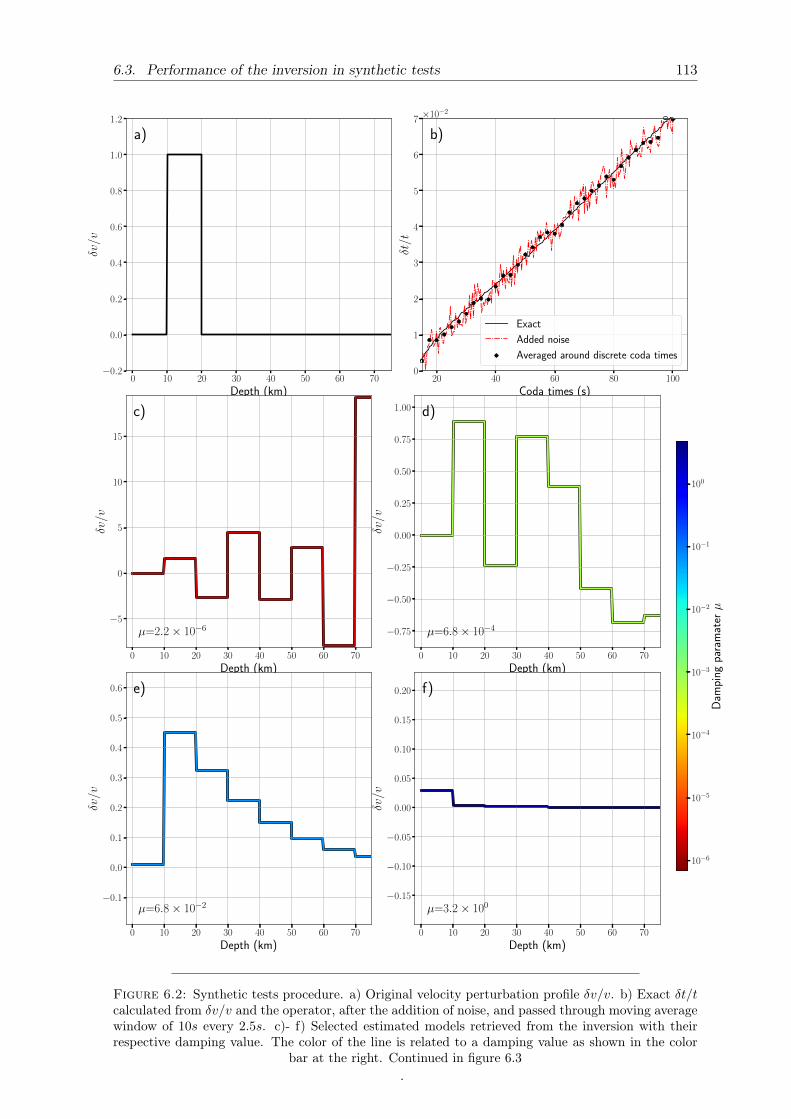
6.3. Performance of the inversion in synthetic tests 113
0 10 20 30 40 50 60 70
Depth (km)
−0.2
0.0
0.2
0.4
0.6
0.8
1.0
1.2
δv/v
a)
20 40 60 80 100
Coda times (s)
0
1
2
3
4
5
6
7
δt/t
×10−2
b)
Exact
Added noise
Averaged around discrete coda times
0 10 20 30 40 50 60 70
Depth (km)
−5
0
5
10
15
δv/v
µ=2.2× 10⁻⁶
c)
0 10 20 30 40 50 60 70
Depth (km)
−0.75
−0.50
−0.25
0.00
0.25
0.50
0.75
1.00
δv/v
µ=6.8× 10⁻⁴
d)
0 10 20 30 40 50 60 70
Depth (km)
−0.1
0.0
0.1
0.2
0.3
0.4
0.5
0.6
δv/v
µ=6.8× 10⁻²
e)
0 10 20 30 40 50 60 70
Depth (km)
−0.15
−0.10
−0.05
0.00
0.05
0.10
0.15
0.20
δv/v
µ=3.2× 100
f)
10−6
10−5
10−4
10−3
10−2
10−1
100
Dam
ping
para
mat
erµ
Figure 6.2: Synthetic tests procedure. a) Original velocity perturbation profile δv/v. b) Exact δt/tcalculated from δv/v and the operator, after the addition of noise, and passed through moving averagewindow of 10s every 2.5s. c)- f) Selected estimated models retrieved from the inversion with theirrespective damping value. The color of the line is related to a damping value as shown in the color
bar at the right. Continued in figure 6.3.

114 Chapter 6. Recovery of velocity variations at depth
10−4 10−3 10−2
Residual norm
10−2
100
102
104
106
Sol
utio
nno
rm
a)10−6 10−5 10−4 10−3 10−2 10−1 100
Damping
100
101
102
Rea
lre
sidu
e
b)
0 10 20 30 40 50 60 70
Depth (km)
−0.2
0.0
0.2
0.4
0.6
0.8
1.0
1.2
δv/v
c)
Original velocity profile
µ=4.6× 10⁻³
10−6
10−5
10−4
10−3
10−2
10−1
100
Dam
ping
para
mat
erµ
Figure 6.3: Synthetic tests procedure, continuation. a) Trade-off curve. Each point represents aninversion. b) Real residue calculated for the same set of estimated models. c) Estimated velocity per-turbations for the best inversion as chosen by the trade-off criteria, along with its damping parameter.This configuration is highlighted in the two upper plots with a black border. The colors of the dots
and line are related to the value of the damping parameter.
6.3. Performance of the inversion in synthetic tests 115
is significant, although in the figure only the first 75km are shown for visualizationpurposes
II. We calculate what would be the exact δt/t measured at the surface making a matrixmultiplication between the model and the full-resolution operator G as schematized inthe equation 6.17. Then we add to this exact δt/t a randomly generated noise. Bothof these sets of δt/t are defined over a dense set of lapse times. To mimic real-lifemeasurements taken from a cross-correlation, we make a moving average going from 15sto 105s, every 2.5s over the δt/t with noise. The three δt/t are shown in figure 6.2b
III. The operator is down-sampled with the averaged lapse times and a new layering (in thiscase, of thickness of 10km )
IV. The inversion is performed following equation 6.7 with a set of damping values thatare chosen to be between the maximum and the minimum singular value of the down-sampled operator. In figures 6.2c-f can be seen the result of 4 of these inversions withtheir respective damping values.
V. For each of these estimated models m we calculate the residual norm ‖Gm − d‖ andthe solution norm ‖m‖ to make a trade-off curve shown in the figure 6.1: in our casethe result of this trade-off curve is shown in the figure 6.3a.
VI. We increase the depth resolution of the estimated model over the more dense set ofdepths (with thickness of 0.2km) to make a direct comparison between the m and mwith the root-mean-square error, for each damping value:
Rr =
√√√√ 1
N
N∑i=0
(δv
v(i)real −
δv
v(i)estimated
)2
(6.21)
where Rr is what we call the real residue and N is the total number of layers. Thesmaller is this value, the closer is the estimated model from the real one. We plot eachdamping value with its respective real residue to compare their performance as shownin figure 6.3b.
VII. Finally, imitating what would be a real case scenario, we chose the model whose dampingvalue is closer to the elbow of the trade-off curve as the correct one. This particularmodel is highlighted with a black border in the plots 6.3a and 6.3b, and is plotted inthe figure 6.3c. In this example this configuration happens to have the smaller realresidue which means that the trade-off criteria is appropriate. Although this won’t benecessarily always the case, in general, this "elbow" configuration is always close to thebest performing one.
This simple example shows the known effect of µ in the inversion: as can be seen in figures6.2c-f, the lowest is the damping parameter the highest is the amplitude and the oscillation ofthe estimated model. Although this parameter helps to damp the estimated model limitingthe influence of noise, it does it sacrificing its resolution. This trade-off behavior can beseen in the plot 6.3a where low damping values result in models with strong oscillations (bigsolution norms) that may be overfitting the presence of noise (low residual norm), whereashigh damping values results in models with weak oscillations (low solution norms) that maynot be fitting good enough to the observations (high residual norm). Before continuing wedefine the zero-residue R0 as the residue that would produce an estimated model in which all(δv/v)estimated = 0:

116 Chapter 6. Recovery of velocity variations at depth
0 25 50 75 100 125 150 175
Depth (km)
0.0
0.2
0.4
0.6
0.8
1.0
δv/v
a)
Original velocity profile
Direct estimation
0 20 40 60 80 100 120 140
Coda times (s)
0.00
0.01
0.02
0.03
0.04
δt/t
b)
Figure 6.4: Direct inversion without artifical noise. a) Real model and estimated model for theinversion made with the full-resolution operator from the δt/t. b) δt/t obtained with the full-resolution
operator
R0 =
√√√√ 1
N
N∑i=0
(δv
v(i)real
)2
=‖m‖√N
(6.22)
This value will be used as a reference point: an estimated model with a higher residuethan R0 has lost all information.
6.3.1 Noise-free inversion: Effects of the downsampling process
We make a control test where no noise is introduced. It consists of estimating the modelusing the full-resolution operator, it means, applying the equation 6.5 directly over d. Theresult of this is shown in figure 6.4a. Although the result shows the presence of fluctuationsmost likely generated by numerical imprecisions, it reproduces the original sharp velocityperturbation. The produced phase perturbations at the surface (figure 6.4b) is consistentwith a wave propagation understanding of the sensitivity: δt/t deviates from zero at laterlapse times because of the seismic field samples progressively deeper zones of the medium,where the perturbation is located. It is worth noticing that this inversion makes full use ofall the available lapse times, a feature that in real applications is not possible.
The next test consists in making the inversion over the averaged measurement of δt/tusing the down-sampled operator, for two cases: the first one, analyzing big perturbations atdepth, and the second case analyzing smaller perturbations close to the surface. In figures6.5a and 6.5b can be seen the real model and the produced δt/t respectively. The originalmodel is the same used in figure 6.4.
In this case the inversion is done with a down-sampled operator over a set of δt/t between15s and 65s, with a spacing of 2.5s between them, represented by the dots in the figure 6.5b;the duration of the window in this moving window average is 10s. The half-space is divided

6.3. Performance of the inversion in synthetic tests 117
0 25 50 75 100 125 150 175
Depth (km)
−0.2
0.0
0.2
0.4
0.6
0.8
1.0
δv/v
a)
Original velocity profile
Direct estimation
µ=1.0× 10⁻⁴
15 20 25 30 35 40 45 50 55
Coda times (s)
0.000
0.001
0.002
0.003
0.004
0.005
0.006
δt/t
b)
Exact
Averaged around discrete coda times
Figure 6.5: Inversion without artificial noise for a deep perturbation. a) Original model, estimatedmodel for the inversion made directly with the down-sampled operator, and estimated model for theinversion made with the down-sampled operator including a damping parameter. b) δt/t obtained
with the full-resolution operator and averaged δt/t around the measurements points.
with a regular layering of 10km spanning from 0km to 180km depth. A first inversion canbe made directly over the averaged δt/t using the down-sampled operator with the equation6.5; this produces the very unstable model estimation represented by the dotted blue line infigure 6.5a. The wide amplitude of this solution seems to suggest that the reduction of theresolution of the data and the operator, acts as a noise introduction in the system. This meansthat its overall effect can be controlled through the introduction of the damping parameter;in effect, making a full set of inversions, and choosing the best one according to the L-curvecriteria (as was described in the previous section), leads to the solution in red in figure 6.5a,which resembles more closely the real model. However, this solution shows already a loss ofresolution which is characteristic of the introduction of the damping parameter. This helpsto illustrate that even in a noise-free scenario, the regularization process is necessary.
Now, we test how the inversion performs over a 1km perturbation within the first kilome-ters of depth, as the one shown in figure 6.6a. The layering of the downsampled operator ishas a thickness of 1km. The generated δt/t and its averaged version are represented by theline and the dots in figure 6.6b respectively; in this case, the δt/t diverges from 0 at an earlylapse time, as expected from a perturbation located close to the surface. As occurred before,the inversion made directly with the down-sampled operator produces a very irregular esti-mation, represented by the blue dotted line in figure 6.6a. However, the introduction of thedamping parameter does not produce a reliable estimation either: in this case, the dampedestimated model (green line in figure 6.6a) does not show any distinctive feature that can berelated to the original perturbation.
To increase the performance of the inversion, we introduce a weighting factor that searchesfor models that have velocity perturbations within the first layers of depth and penalizessolutions that show fluctuations at deeper levels. The idea is to prioritize solutions that liein what would be the crust, and ignore the rest; this is a reasonable expectation as most

118 Chapter 6. Recovery of velocity variations at depth
0 5 10 15 20 25 30
Depth (km)
0.0
0.2
0.4
0.6
0.8
1.0
δv/v
a)
Original velocity profile
Direct estimation
µ=3.2× 10⁻⁴
Depth pen., µ=1.0× 10⁻⁴
20 30 40 50 60
Coda times (s)
0.001
0.002
0.003
0.004
0.005
0.006
δt/t
b)
Exact
Averaged around discrete coda times
Figure 6.6: Inversion without artificial noise for a shallow perturbation. a) Original model andestimated models for the inversion made directly with the down-sampled operator, with the down-sampled operator including a damping parameter, and with the down-sampled operator including adamping parameter and a depth penalization. b) δt/t obtained with the full-resolution operator and
averaged δt/t around the measurements points.
0 5 10 15 20 25 30
Depth (km)
2
4
6
8
10
L
Figure 6.7: Depth penalization on the parameters in the model. Sigmoid function centered around15km. The higher is the value, the stronger will be the minimization process on the estimated model
at this depth.
6.3. Performance of the inversion in synthetic tests 119
of the known factors that generate fluctuations in the δt/t come from phenomena locatedwithin these first kilometers of the crust, like earthquakes and weather-related cycles. In thepractice, this is done multiplying m with a smooth sigmoid function L (equation 6.10) thatleaves the component of m equal if it is located between 0km and 15km, but penalizes themby a factor of 10 if they are at deeper levels than this threshold. This function can be seenin figure 6.7. The introduction of the associated matrix Wm in the equation 6.12 producesthe solution represented by the red line in figure 6.6a. This increases the capacity of theinversion to resolve thinner perturbations, at the expense of being unable to locate changesat a deeper layer. In a practical setting, a simultaneous inversion for deep thick velocitystructures, complemented with other for thin shallow ones, should be enough to obtain acomprehensive set of observations of the dynamic in the medium.
6.3.2 Performance at different depths
The performance of the inversion is tested moving the perturbation at depths without artificialnoise. The used set of measurements δt/t ranges from 15s to 65s every 2.5s. The result of someselected depths is shown in figure 6.8. As we move deeper, the best performant configuration(as selected by the L-curve criteria) is generated by a systematically lower damping parameter.This indicates that when the perturbation is close to the surface the estimated models aremore robust but have less resolution. Figure 6.8b shows a case where the velocity perturbationis located between two layers of the inversion, which leads to more unstable results.
Figure 6.9a shows the residues (equation 6.21) for different depths without noise: theoscillation is generated by the location of the perturbation between layers, having the lowervalues when the perturbation is aligned to the layering. At deeper levels, the residue ofthe aligned cases is progressively lower as these configurations use a lower damping value,that produces higher resolution estimations. In figure 6.9b we see the residues of a set ofinversions under the same conditions but with an artificial level of noise added to the δt/t;the residues increase at depth as the noise make the less robust inversions unstable. Below80km there are no more residues because for these configurations the trade-off curve doesnot have anymore its characteristic L-shape, and therefore, it is impossible to know what isthe best configuration between different damping parameters. This is also a sign of the lowquality of the estimations. Interestingly enough, this suggests that the level of noise limitsthe practical reach of the inversion, as will be seen afterwards in detail. In the case wherethere is no noise, the inversion seems to reach a limit at around 110km location at whichthe sensitivity values are too low. it is worth mentioning that the big instabilities that areproduced when the perturbation is close to the surface between layers (at depths of 2km,4km, and 6km to be precise) are one of the reasons why a second configuration with thinnerlayers is analyzed independently.
Figure 6.10 illustrates how the noise weakens and can drown completely the informationcontained in the perturbation of the phase. The δt/t for the deeper layer is around one orderof magnitude smaller that for the shallow layer, which makes it more susceptible to the noise;the noise amplitude for the former is comparable with the changes in δt/t, and therefore,almost all the information is gone.
The same analysis is performed over the inversion with thinner and shallower layers,making use of the depth penalization in the minimization as was previously explained. In thiscase, the perturbation has 1km thickness and is shifted by steps of 200m. The half-space isdivided into layers of 1km. Four selected inversions are shown in figure 6.11 (a fifth one canbe seen in figure 6.6a). The inversion shown in 6.11a is made for a perturbation that is notaligned with the layering, and contrary to what we saw in the thicker case, this does not leadto an unstable estimation. We see as in the first case, a migration of the damping parameter
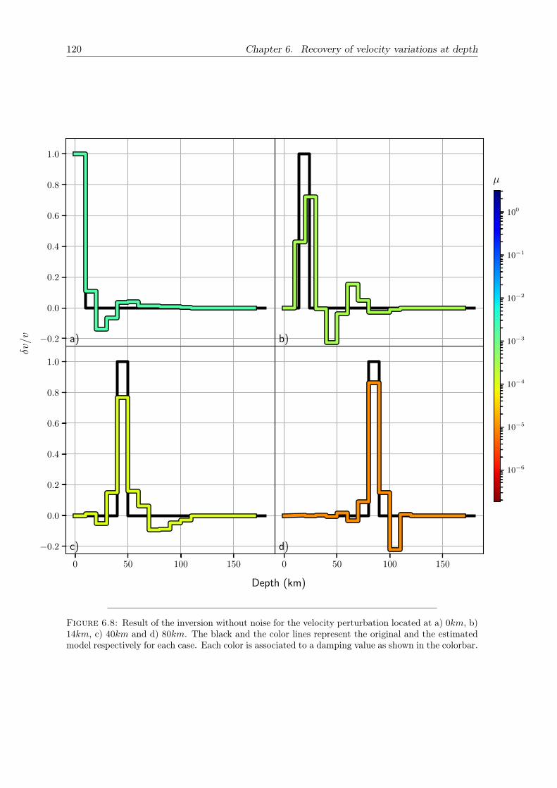
120 Chapter 6. Recovery of velocity variations at depth
0 50 100 150
−0.2
0.0
0.2
0.4
0.6
0.8
1.0
b)
10−6
10−5
10−4
10−3
10−2
10−1
100
µ
0 50 100 150
−0.2
0.0
0.2
0.4
0.6
0.8
1.0
d)
0 50 100 150
−0.2
0.0
0.2
0.4
0.6
0.8
1.0
a)
0 50 100 150
−0.2
0.0
0.2
0.4
0.6
0.8
1.0
c)
δv/v
Depth (km)
Figure 6.8: Result of the inversion without noise for the velocity perturbation located at a) 0km, b)14km, c) 40km and d) 80km. The black and the color lines represent the original and the estimatedmodel respectively for each case. Each color is associated to a damping value as shown in the colorbar.

6.3. Performance of the inversion in synthetic tests 121
0 20 40 60 80 100 120
Depth of the perturbation (km)
0.0
0.2
0.4
0.6
Res
idue
a)
0 20 40 60 80 100 120
Depth of the perturbation (km)
0.0
0.2
0.4
0.6
Res
idue
b)
Figure 6.9: Real residue for the perturbation at several depths for a system a) without noise b)withadded artificial noise of 10−3 of amplitude. The dashed line marks the value of R0.
towards lower values when inverting for deeper layers. However, the general resolution of allthe solutions is lower and the estimations seem to be poorly located. When the perturbationis located below 9km (6.11d), it appears a bias in the estimated model because at this depthit starts increasing the amplitude of the sigmoidal penalization function (shown in figure 6.7.
The residue plot for the cases with and without noise (figure 6.12) lead to similar conclu-sions as before: the addition of noise limits the reach of the inversion, in this case, shorteningthe range that was set by the depth penalization. In the first kilometer is present the oscil-lation generated when the perturbation is not aligned with the layering system. However, inthis case, we obtain an acceptable estimation as the residue values are below R0.
6.3.3 Performance with different lapse times
Next, we analyze an important question: how the coda window duration used in the inversionaffects the final model estimation. To test this, we use a perturbation fixed at 50km depth, andwe start with a set of measurements of δt/t that goes from 15s to 45s. Then we progressivelyadd a new δt/t measurements at later coda times (47.5s, 50s, ...) and redo the inversion. Thismeans the segment of the coda used begins always at 15s but finish a different lapse times;this last lapse time will be used as the identifier of the set. This process mimics what wouldbe a real case-scenario where the length of the coda time to include in the apparent δv/v atthe surface is usually chosen with a trial-and-error process.
A sample of two inversions with different coda times sets is shown in figure 6.13. Thesetwo estimated solutions show a general behavior: using a smaller set of lapse times leads tosolutions with a lower damping parameter, and therefore, more sensitive to noise. However,when using lower coda segments what is gained in robustness is lost in resolution. This canalso be seen in figure 6.14a where the residue increases with the number of measurements,because of this loss of precision. As expected, this tendency in the residue is reversed whennoise is introduced as shown in 6.14b: the inversions made with the smaller lapse time sets,i.e., using a smaller section of the coda, produce unstable model estimations. Although thislast plot suggests that after adding 60s to the set of δt/t the results are almost the same,in reality, there are important quantitative differences between them, as can be seen in thefigure 6.15. This shows that the residue estimation, although useful, is not the best way toassess the performance of the inversion when the features of the system are being smoothedat very different degrees. The case with the thinner and shallower perturbations shows thesame trends (longer lapse times leads to more robust and smoothed solutions) and therefore
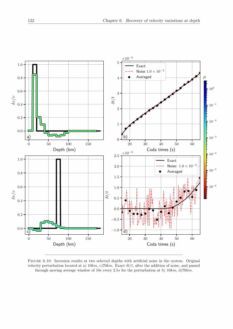
122 Chapter 6. Recovery of velocity variations at depth
0 50 100 150
Depth (km)
0.0
0.2
0.4
0.6
0.8
1.0
δv/v
a)
20 30 40 50 60
Coda times (s)
0
1
2
3
4
5
δt/t
×10−2
b)
10−6
10−5
10−4
10−3
10−2
10−1
100
µ
Exact
Noise 1.0× 10⁻³
Averaged
0 50 100 150
Depth (km)
0.0
0.2
0.4
0.6
0.8
1.0
δv/v
c)
20 30 40 50 60
Coda times (s)
−1.0
−0.5
0.0
0.5
1.0
1.5
2.0
2.5
δt/t
×10−3
d)
Exact
Noise: 1.0× 10⁻³
Averaged
Figure 6.10: Inversion results at two selected depths with artificial noise in the system. Originalvelocity perturbation located at a) 10km, c)70km. Exact δt/t, after the addition of noise, and passed
through moving average window of 10s every 2.5s for the perturbation at b) 10km, d)70km.

6.3. Performance of the inversion in synthetic tests 123
0 5 10 15
−0.2
0.0
0.2
0.4
0.6
0.8
1.0
b)
10−5
10−4
10−3
10−2
10−1
100
µ
0 5 10 15
−0.2
0.0
0.2
0.4
0.6
0.8
1.0
d)
0 5 10 15
−0.2
0.0
0.2
0.4
0.6
0.8
1.0
a)
0 5 10 15
−0.2
0.0
0.2
0.4
0.6
0.8
1.0
c)
δv/v
Depth (km)
Figure 6.11: Result of the inversion without noise for the velocity perturbation located at a) 0.4km,b) 4km, c) 6km and d) 11km. The black and the color lines represent the original and the estimatedmodel respectively for each case. Each color is associated to a damping value as shown in the colorbar.
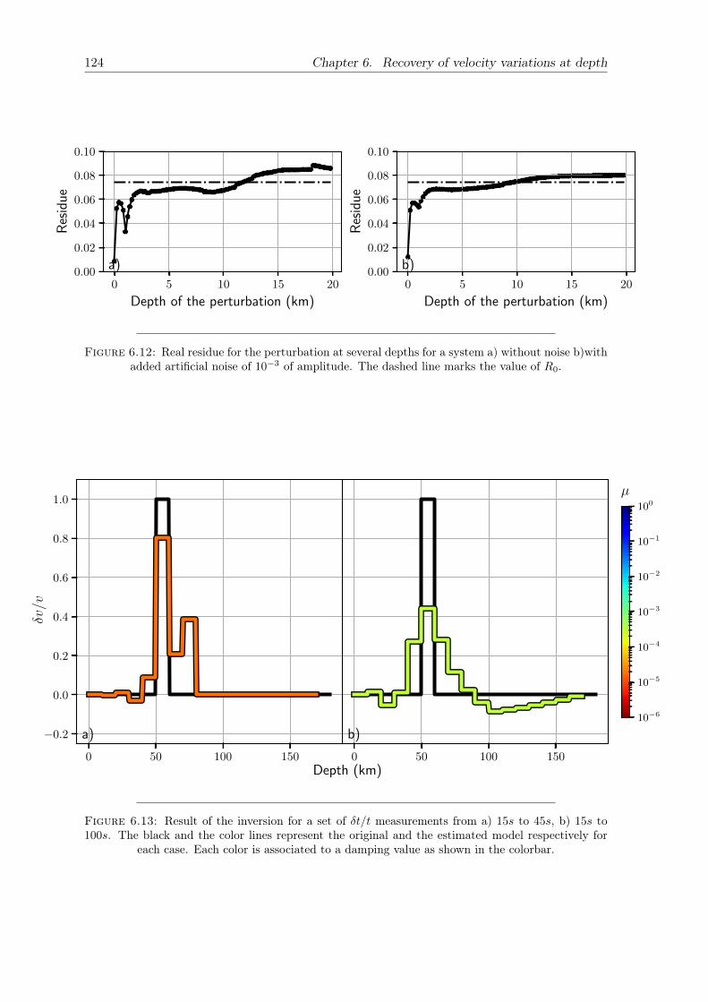
124 Chapter 6. Recovery of velocity variations at depth
0 5 10 15 20
Depth of the perturbation (km)
0.00
0.02
0.04
0.06
0.08
0.10
Res
idue
a)
0 5 10 15 20
Depth of the perturbation (km)
0.00
0.02
0.04
0.06
0.08
0.10
Res
idue
b)
Figure 6.12: Real residue for the perturbation at several depths for a system a) without noise b)withadded artificial noise of 10−3 of amplitude. The dashed line marks the value of R0.
0 50 100 150
−0.2
0.0
0.2
0.4
0.6
0.8
1.0
b)10−6
10−5
10−4
10−3
10−2
10−1
100
µ
0 50 100 150
−0.2
0.0
0.2
0.4
0.6
0.8
1.0
a)
δv/v
Depth (km)
Figure 6.13: Result of the inversion for a set of δt/t measurements from a) 15s to 45s, b) 15s to100s. The black and the color lines represent the original and the estimated model respectively for
each case. Each color is associated to a damping value as shown in the colorbar.

6.3. Performance of the inversion in synthetic tests 125
40 60 80 100 120
Last lapse time (s)
0.0
0.1
0.2
0.3
Res
idue
a)
40 60 80 100 120
Last lapse time (s)
0.0
0.1
0.2
0.3
Res
idue
b)
Figure 6.14: Real residue for different lapse time ranges starting at 15s and ending at the lapse timegiven in the horizontal axis a) without noise b) with added artificial noise of 10−3 of amplitude. The
dashed line marks the value of R0.
are not shown. However, as in that case the solutions are already smoothed, adding too manymeasurements of δt/t may degrade critically the resolution of the model. This also meansthat this case is even more sensitive to noise.
6.3.4 Performance with different levels of noise
Let’s think that we generate a perturbation at a certain depth and that we try to retrieve itthrough the inversion. We know that the quality of the estimated model will depend on thelevel of noise that we add to the system; in fact, we have seen that if we keep increasing thelevel of noise systematically, at some point the information of the δt/t is completely lost andthe inversion will be unable to retrieve the original model. Even more, we saw that this alsodepends on the depth of the layer as that may change the amplitude of the δt/t itself.
We want to find for each depth the maximum level of noise under which the inversionmakes an acceptable job. For this, we make a series of inversions using always the codabetween between 15s and 125s. We proceed as follows: we create a perturbation of 10km andcalculate the zero-residue R0. We choose a value a bit lower, 0.92R0, as a symbolic thresholdunder which the results are still acceptable. Now, with the perturbation located at a certaindepth, we proceed to perform inversions increasing gradually the level of noise in the system.Once the residue threshold is reached, the noise amplitude is registered: this is the maximumamplitude of noise that the system can tolerates at this depth. However, this maximumamplitude may be different for the same model with different realizations of the noise givenits random nature. For this reason, the process is repeated for the same model with 50different realizations of noise, and all the maximum-amplitudes are averaged between them.Finally, the whole operation is repeated for the perturbation located at another position. Themaximum amplitude of the noise for each depth is shown as the scatter plot in figure 6.16. Itis clear that the deeper is the perturbation, the lower is the maximum level of noise that canintroduce into the system without losing the original information. However, the interestingaspect of this behavior is that the maximum tolerable amplitude of noise can be related tothe sensitivity kernel itself.
From 6.17 can be seen that an unitary perturbation at different positions produce mea-surements of δt/t that are proportional to the the sensitivity. As the noise is added to theδt/t, its effect on the inversion depends on to the relative amplitudes between the two: ifthe sensitivity is high compared with the level of noise, most of the features of the δt/t are
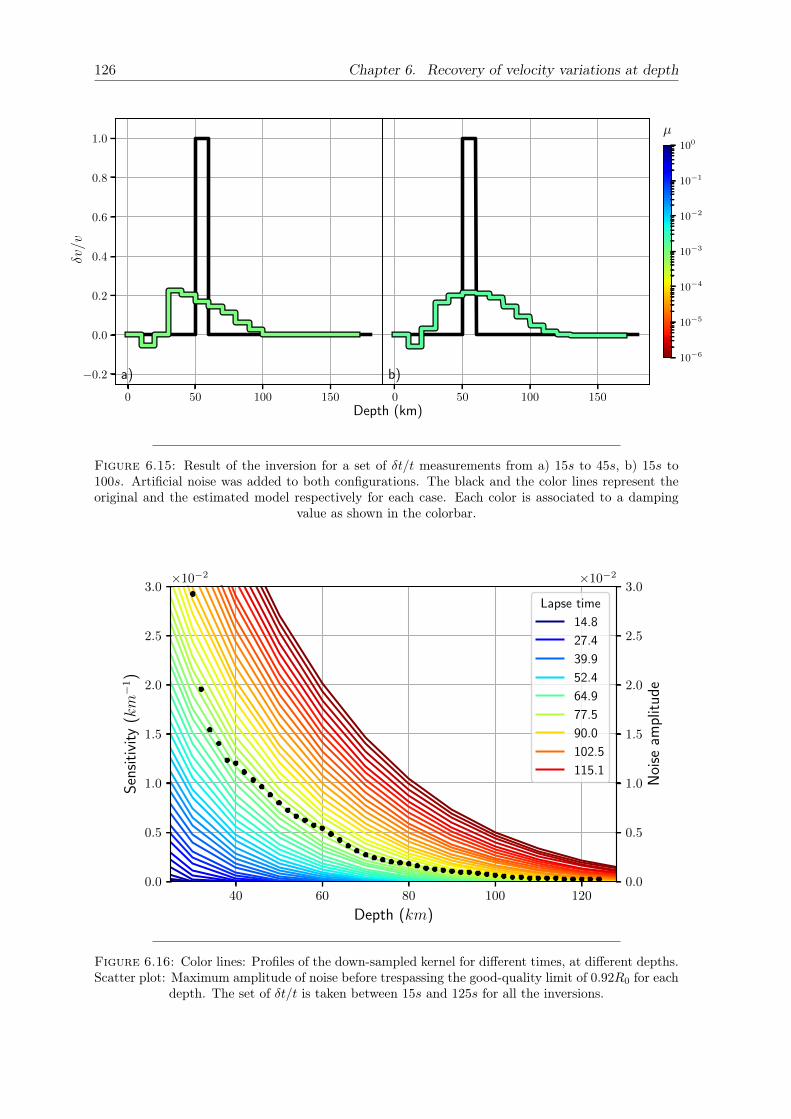
126 Chapter 6. Recovery of velocity variations at depth
0 50 100 150
−0.2
0.0
0.2
0.4
0.6
0.8
1.0
b)10−6
10−5
10−4
10−3
10−2
10−1
100
µ
0 50 100 150
−0.2
0.0
0.2
0.4
0.6
0.8
1.0
a)
δv/v
Depth (km)
Figure 6.15: Result of the inversion for a set of δt/t measurements from a) 15s to 45s, b) 15s to100s. Artificial noise was added to both configurations. The black and the color lines represent theoriginal and the estimated model respectively for each case. Each color is associated to a damping
value as shown in the colorbar.
40 60 80 100 120
Depth (km)
0.0
0.5
1.0
1.5
2.0
2.5
3.0
Sen
siti
vity
(km−
1)
×10−2
Lapse time
14.8
27.4
39.9
52.4
64.9
77.5
90.0
102.5
115.1
0.0
0.5
1.0
1.5
2.0
2.5
3.0
Noi
seam
plit
ude
×10−2
Figure 6.16: Color lines: Profiles of the down-sampled kernel for different times, at different depths.Scatter plot: Maximum amplitude of noise before trespassing the good-quality limit of 0.92R0 for each
depth. The set of δt/t is taken between 15s and 125s for all the inversions.

6.4. Conclusions 127
preserved and the inversion performs well. If both are comparable, the behavior of the δt/t ismasked and it is impossible to recover the velocity perturbation with the inversion. In figure6.16 is also plotted the kernel profile for different times at different depths, which shows thisproportionality. This means that the maximum level of noise that we can add to the systemwithout losing completely the information is a fraction of the maximum sensitivity at thatpoint. This practical relation can be quite useful to determine the possibilities of retrievinginformation at a certain depth, by analyzing the kernel profile and the general level of noisein the signals.
Nonetheless, it must be pointed out that the actual proportion between the amplitude ofthe noise and the amplitude of the sensitivity may be altered by the actual value of the velocityperturbation (that will be a number much smaller than 1) and by the averaging process inthe temporal dimension that may affect the effective noise amplitude of the system. Below30km the relation does not hold because at those depths there is a dramatic change in thesensitivity due to the surfaces waves and because the shape itself of the δt/t may change a lotand be quite different from the characteristic shape generated by having the perturbation atdepth (see for example 6.5b). Finally, this same analysis cannot be done close to the surfacewith the surface waves sensitivity because the parameter we use to determine the quality ofthe inversion (the residue Rr) does not work well with smoothed shapes as was seen in theprevious section.
6.4 Conclusions
Based on the scalar model that couples body and surface waves, a linear relationship can beestablished between the changes of velocity on the crust, and the changes of phase in the cross-correlations obtained by seismic-noise based methods at the surface: this is the sensitivitykernel. This particular kernel is obtained for the case where the source and the receiverare located at the same position. With it we can construct a discrete matrix operator thatconnects a series of measurements δt/t, with its sources δv/v. However, this first operator isdefined over a dense set of lapse times and depths, and in practice, we have a limited number ofobservations. We discuss the process to reduce the dimensions of this full-resolution operatorto obtain a down-sampled version that is the one that we would use in applications.
We design a general procedure under which we test the performance and limitations of theinversion. This is based on obtaining an estimated model for a range of values of the dampingparameter, and choosing automatically the best one following the L-curve criteria. We testthe precision of the criteria calculating the residual difference between the original modeland the estimated model and observe an overall good performance. We also conclude thatdownsampling the set of measurements available for the inversion acts like a noise introductionin the system. Therefore the utilization of the damping parameter is necessary. However, thishas as side-effect the inevitable loss of resolution of the original model.
We separate the analysis in two systems of layering of 10km and 1km thick, and we useperturbations of similar size (10km and 1km respectively) to test the inversion. The secondone is desgined to image interesting phenomena like seismic events or seasonal-driven fluidmovements in the crust, that happen in the first kilometers close to the surface. The use ofthe damping parameter is not sufficient to recover the original model in the thinner layeringsystem. To increase the capacity of the inversion the introduce a penalization function thatprioritize solutions with perturbations located in the first layers of the half-space. This is donethrough a smooth sigmoid function that assigns a larger weight to the deeper parametersof the model in the minimization process of the least square solution. We find that this
128 Chapter 6. Recovery of velocity variations at depth
depth penalization helps us to retrieve the location of the original perturbation, although theestimated models are of lower resolution.
The performance of the inversion is tested when the perturbation is located at differentdepths. We find that in noise-free conditions, the deeper is the δv/v the lower is the dampingvalue of the estimated model. This has two main implications: first, it means on theseconditions the estimated model at depth is a bit more precise than close to the surface, wherethe estimations are smoother. The second one is that closer to the surface the solutions areless vulnerable to the effect of the noise. In effect, we find that the introduction of an artificialrandom generated noise in the system leads to a dramatic loss of precision when we are tryingto resolve the velocity structure deeper in the medium. This effect is so strong, that there isa depth after which the original information is completely lost. This is product of the levelsof δt/t falling under the levels of noise, or in other words, of a low signal-to-noise ratio. Thissame behavior is observed in the thinner layering system, with the difference that on this casethe maximum depth to which the inversion can recover the perturbation is determined by thepenalization sigmoid function.
We are also interested in knowing how the duration of the coda used in the inversion affectsthe quality of the calculated models. For this, we compare the results of a series of inversions,that use a progressively bigger set of measurements of δt/t. This is done by attaching anew measurement in a slightly later lapse time. Both cases (the thicker and thinner layeringsystem) show that the smaller is the number of measurements, the lower is the dampingvalue of the estimated model; as before, this leads to models with higher precision but quiteunstable to the introduction of noise. A large set of measurements will generate very stableresults that have unfortunately lower resolution. In the practice making tests starting with alarge number of δt/t measurements, could reveal the presence of structures, that can after beresolved with higher resolution decreasing progressively the used coda in the inversion. In thethinner layering case, the use of long segments of the coda can deteriorate beyond recognitionthe velocity perturbations, so in that case the search of the equilibrium point between stabilityand precision should start with the smallest possible set of δt/t.
Finally, the overall role of the noise in the inversion is analyzed. For each depth, wemake a series of inversions where the noise is gradually increased until the original velocityperturbation is almost completely gone. This is the maximum level of noise that the systemcan tolerate without losing completely the information. We find that in general, this levelis proportional with the sensitivity. This gives a very convenient tool to assess the eventualrobustness of the inversion based on the characteristics of the kernel itself. However this doesnot hold for points close to the surface due to the presence of the surface waves, and to thevaried shapes that the δt/t takes in those regions
129
Chapter 7
Conclusions and perspectives
We present in this thesis a study focus on the development of tools for the analysis of ambientseismic noise. Our main interest is to have a deeper understanding of the mechanisms thatare responsible for the well-known velocity perturbations of the seismic waves in the crust.This means separating and localizing each of these processes with the information that isusually recorded on the surface. In the first part, we analyzed a particular case in the southof Italy. This region shows a very particular set of characteristics that makes it an interestingstudy case: the presence of an aquifer, a limited period of seismic activity that included slowslip events and a M5.0 earthquake, and a convenient deployment of GPS and meteorologicalstations along with a seismic station located very close to the fault system. We proposedsome simple physical models that allow us to predict the observed velocity variations in thezone from the rainfall of the region, and validate our physical interpretation of the processinside the crust with geodetic data. We successfully separate and recognize the independentinfluence of seasonal and tectonic phenomena in the measurements obtained from the analysisthe ambient seismic noise.
On the other hand, we address one of the main objectives of Passive Image Interferometry:localize the changes in the crust from the phase delays registered at the surface. This objectiveis complementary to the previous analysis as we expect that different processes affect differentparts of the crust. We develop this part of the project in three stages: the study of ascalar model that allows the coupling between surface and body waves, the estimation of thesensitivity kernel of this system, and the technical study of inverse problem with this kernelto locate velocity perturbations in a real-life like scenario.
In the first stage, we use a scalar model with a mixed boundary condition that sustainsthe natural propagation of surface waves. We study the scattering cross sections betweenall the possible combinations of propagation in this system, and from it, we estimate thescattering mean free times. Based on this we construct the radiative transfer equations of thesystem and test them in a Monte Carlo simulation. The results show that the scalar modelreproduces expected behaviors in the limit cases, and gives us an insightful perspective of theenergy exchange between body and surface waves in the first stages of propagation after theactivation of an impulsive source.
In the second stage, we reconstruct the sensitivity framework including the directionalityof the energy and add into it the two modes of propagation. At the same time, we usea variational approach to quantify how a velocity perturbation in the medium affects thepropagation velocity of the surface waves. We use once again Monte Carlo simulations, thistime to estimate the travel-time distribution of the energy when propagating from a sourceto a receiver, both of them located at the same spot on the surface. All of these results areintegrated into the construction of a sensitivity kernel that accounts simultaneously for bothtypes of waves. Basic tests on this newly found kernel found good agreement with previousresults based on full wavefield elastic simulations and theoretical solutions in 3-D full spacepropagation. However, we also observe disagreements related to the evolution of the system,

130 Chapter 7. Conclusions and perspectives
caused by the introduction of the coupling or exchange region delimited by the penetrationof the surface waves. Furthermore, we find evidence that shows that the coupled system isinvariant when the ratio between the mean free path and the penetration depth of the surfacewave is maintained.
Finally, in the third stage, we study the capabilities and limitations of the kernel toidentify velocity variations in the crust under real-life conditions within the framework of theinverse problem. In this section, we focus on the effect of three variables within the inversion:the depth of the perturbation, the duration of the coda segment to invert, and the level ofnoise in the system. We find useful relations for each of these cases to make a more effectiveinterpretation of the result of an inversion performed with the scalar sensitivity kernel.
In figure 7.1 we present a first result of the inversion over measurements of δt/t obtainedfrom the station MMNO in the region of Pollino, Italy, described in Chapter 3. On top,we have the apparent velocity variation, and at the bottom the actual velocity variation inthe crust for several depths, ranging from 0km to 1.2km depth. Each of these curves wassmoothed using a moving average of 10 days. The parameters used for the measurements ofthe time densities are shown in table 6.1 on page 112. We use a frequency band between 0.5Hzand 1.0Hz and measurements of the apparent velocity variation obtained with the MovingCross Spectral Window technique between 10s and 40s each 0.4s with a window of 8s aroundeach lapse time. The apparent velocity variation is usually obtained with the average betweenall the possible correlations between the three available channels for the stations. However,for the inversion, we use only the measurements of δt/t of the correlation North-North as itshows the closest estimations to the final apparent velocity variation
For each day we have a measurement of values of δt/t and therefore the inversion isperformed for each date independently. This means that the damping parameter chosenautomatically with the L-curve criteria may be different for different days; however, in figure7.1 we present the inversion made with the average damping parameter obtained from all thedates. This decision is justified if we recognize that the velocity perturbations appear andremain in the same position in the crust over long lapse times, in this case, in the order ofmonths. This allows us to obtain results from days when the trade-off curve of the inversionis poor. In this case, the perturbations in the medium seem to be constrained to the firstkilometers of depth. This is possibly a consequence of the predominance of the surface waveson this part of the coda: when normalize by the body-to-body mean free time, the later lapsetime 40s is equal to t/τb→b = 1.39, a very early stage of the system where the sensitivity of thesystem is almost completely determined by the surface wave sensitivity (see figure 5.12 on page100). However, the recovered model shows an interesting feature: from some times before theearthquake (September-October 2012), until the reported last slow slip event in the zone (mid2013, see figure 3.3 on page 26) the velocity variation passes through its strongest decrease ofthe whole 10-year period, accentuated by an overall decrease of the natural fluctuation of thetime series. Although the behavior at depth is not really distinctive, the inversion seems tohighlight the period in which there is the most notable stress redistribution of the zone.
Figure 7.2 shows the results of the inversion at deeper zones of the medium. These firstresults indicate that the annual variations and long-term trend are associated with the mostsuperficial layers, more precisely the first kilometer. This is in line with our interpretationin terms of the filling of the karstic system. Note that these fluctuations are not incorrectlyprojected at depth. Unfortunately, due to the dominance of the sensitivity of surface waves,the effects of changes in the deep layers are of small amplitude at short lapse times andour measurements seem to be contaminated by errors that are projected at depth. At thisstage it is clear that these instabilities in the delay measurements need to be reanalyzedand reduced by extended time averaging and by the use of noise reduction techniques suchas those proposed by Baig, Campillo, and Brenguier (2009) or Moreau et al. (2017). We

Chapter 7. Conclusions and perspectives 131
1.50
1.75
2.00
2.25
t/t
Apparent velocity variation
2010 2011 2012 2013 2014 2015 2016 2017 2018 2019
0.6
0.5
0.4
0.3
0.2
0.1
0.0
0.1
v/v
0.0km0.4km0.8km1.2km
Figure 7.1: Top: average apparent velocity variation measures from continuous seismic recordsin the station MMNO at Pollino, Italy. Bottom: velocity variation at several depths obtainedfrom the inversion. A shift of 0.2 was added between them for visualization purposes. The dashed
line marks the date of the M5.0 seismic event.

132 Chapter 7. Conclusions and perspectives
−0.20
−0.15
−0.10
−0.05
0.00
0.05
0.10
δv/v
−0.1
0.0
0.1
App
aren
tve
loci
tyva
riat
ion
(%)
2010 2011 2012 2013 2014 2015 2016 2017 2018 2019
0
1
2
3
4
5
Dep
th(km
)
Figure 7.2: Top: average apparent velocity variation measures from continuous seismic recordsin the station MMNO at Pollino, Italy. Bottom: velocity variation at several depths obtainedfrom the inversion with their values indicated by the colorbar. The dashed line marks the date
of the M5.0 seismic event.

Chapter 7. Conclusions and perspectives 133
will also consider using the continuous wavelet method of Mao et al. (2020) in place of theMWCS method considered so far. Prior to these studies we cannot conclude on a possibletectonic origin of the differences observed in Chapter 3 between observations and modelsderived from meteorological observations. It is also clear that in situation where the surfacewave sensitivity is strong, it could be mandatory to use measurements in different frequencybands to constraint the depth distribution of the changes.
There are many directions of improvement for the work here presented, that go fromconceptual aspects like the introduction of two types of body wave modes of propagationor the development and estimation of the sensitivity kernel for a full-spatial description, totechnical aspects like the use of dense seismic networks or more advance methods for theinversion. The first results show encouraging aspects that may lead in the future to accurateapplications of ambient seismic noise as a regular imaging tool of the crust.

135
Bibliography
Abubakirov, I R and A A Gusev (1990). “Estimation of scattering properties of lithosphereof Kamchatka based on Monte-Carlo simulation of record envelope of a near earthquake”.In: Physics of the Earth and Planetary Interiors 64.1, pp. 52–67. issn: 0031-9201. doi:https://doi.org/10.1016/0031-9201(90)90005-I. url: http://www.sciencedirect.com/science/article/pii/003192019090005I.
Akasaka, Chitoshi and Shigetaka Nakanishi (2000). “Correction of background gravity changesdue to precipitation: Oguni geothermal field, Japan”. In:
Aki, K and P G Richards (2002). Quantitative Seismology, 2d Ed. University Science Book.Aki, Keiiti (1969). “Analysis of the seismic coda of local earthquakes as scattered waves”.
In: Journal of Geophysical Research (1896-1977) 74.2, pp. 615–631. issn: 0148-0227. doi:https://doi.org/10.1029/JB074i002p00615. url: https://doi.org/10.1029/JB074i002p00615.
— (1973). “Scattering of P Waves under the Montana Lasa”. In: J. Geophys. Res. 78.8,pp. 1334–1346.
Akkermans, E and G Montambaux (2007). Mesoscopic Physics of Electrons and Photons.Cambridge: Cambridge University press.
Amoruso, A et al. (2014). “Correlation between groundwater flow and deformation in thefractured carbonate Gran Sasso aquifer (INFN underground laboratories, central Italy)”.In: Water Resources Research 50.6, pp. 4858–4876. doi: https://doi.org/10.1002/2013WR014491. url: https://agupubs.onlinelibrary.wiley.com/doi/abs/10.1002/2013WR014491.
Amos, Colin B et al. (2014). “Uplift and seismicity driven by groundwater depletion incentral California”. In: Nature 509.7501, pp. 483–486. issn: 1476-4687. doi: 10.1038/nature13275. url: https://doi.org/10.1038/nature13275.
Argus, Donald F, Yuning Fu, and Felix W Landerer (2014). “Seasonal variation in totalwater storage in California inferred from GPS observations of vertical land motion”. In:Geophysical Research Letters 41.6, pp. 1971–1980. doi: 10.1002/2014GL059570. url:https://agupubs.onlinelibrary.wiley.com/doi/abs/10.1002/2014GL059570.
ARPACAL. Centro funzionale multirischi della Calabria. http://www.cfd.calabria.it/. url:http://www.cfd.calabria.it/.
Aster, Richard C, Brian Borchers, and Clifford H Thurber (2018). Parameter estimation andinverse problems. Elsevier.
Baig, Adam M, Michel Campillo, and Florent Brenguier (2009). “Denoising seismic noise crosscorrelations”. In: Journal of Geophysical Research: Solid Earth 114.B8.
Bal, Guillaume, George Papanicolaou, and Leonid Ryzhik (2000). “Probabilistic Theory ofTransport Processes with Polarization”. In: SIAM Journal on Applied Mathematics 60.5,pp. 1639–1666. issn: 00361399. url: http://www.jstor.org/stable/3061704.
Bawden, Gerald W et al. (2001). “Tectonic contraction across Los Angeles after removal ofgroundwater pumping effects”. In: Nature 412.6849, pp. 812–815. issn: 1476-4687. doi:10.1038/35090558. url: https://doi.org/10.1038/35090558.

136 Bibliography
Ben-Menahem, Ari and Sarva Jit Singh (1981). Seismic Waves and Sources. isbn: 978-1-4612-5858-2. doi: 10.1007/978-1-4612-5856-8. url: http://link.springer.com/10.1007/978-1-4612-5856-8.
Bergman, Theodore L et al. (2011). Fundamentals of heat and mass transfer. John Wiley andSons.
Beroza, Gregory C, Alex T Cole, and William L Ellsworth (1995). “Stability of coda waveattenuation during the Loma Prieta, California, earthquake sequence”. In: Journal of Geo-physical Research: Solid Earth 100.B3, pp. 3977–3987. issn: 0148-0227. doi: https://doi.org/10.1029/94JB02574. url: https://doi.org/10.1029/94JB02574.
Borsa, Adrian Antal, Duncan Carr Agnew, and Daniel R Cayan (2014). “Ongoing drought-induced uplift in the western United States”. In: Science 345.6204, pp. 1587–1590. issn:0036-8075. doi: 10.1126/science.1260279. url: https://science.sciencemag.org/content/345/6204/1587.
Brenguier, F et al. (2008a). “Postseismic Relaxation Along the San Andreas Fault at Parkfieldfrom Continuous Seismological Observations”. In: Science 321.5895, 1478 LP –1481. doi:10.1126/science.1160943. url: http://science.sciencemag.org/content/321/5895/1478.abstract.
Brenguier, Florent et al. (2008b). “Towards forecasting volcanic eruptions using seismic noise”.In: Nature Geoscience 1.2, pp. 126–130. issn: 1752-0908. doi: 10.1038/ngeo104. url:https://doi.org/10.1038/ngeo104.
Campillo, Michel (2006). “Phase and Correlation in ‘Random’ Seismic Fields and the Re-construction of the Green Function”. In: pure and applied geophysics 163.2, pp. 475–502.issn: 1420-9136. doi: 10.1007/s00024-005-0032-8. url: https://doi.org/10.1007/s00024-005-0032-8.
Campillo, Michel and Anne Paul (2003). “Long-Range Correlations in the Diffuse SeismicCoda”. In: Science (New York, N.Y.) 299, pp. 547–549. doi: 10.1126/science.1078551.
Carcolé, E and H Sato (2010). “Spatial distribution of scattering loss and intrinsic absorptionof short-period s waves in the lithosphere of japan on the basis of the multiple lapse timewindow analysis of hi-net data”. In: Geophysical Journal International 180, pp. 268–290.
Chanard, K et al. (2014). “Modeling deformation induced by seasonal variations of continen-tal water in the Himalaya region: Sensitivity to Earth elastic structure”. In: Journal ofGeophysical Research: Solid Earth 119.6, pp. 5097–5113. doi: 10.1002/2013JB010451.url: https://agupubs.onlinelibrary.wiley.com/doi/abs/10.1002/2013JB010451.
Chapman, Sydney, Thomas George Cowling, and David Burnett (1990). The mathematicaltheory of non-uniform gases: an account of the kinetic theory of viscosity, thermal conduc-tion and diffusion in gases. Cambridge university press.
Cheloni, Daniele et al. (2017). “Aseismic transient during the 2010-2014 seismic swarm: evi-dence for longer recurrence of M >/= 6.5 earthquakes in the Pollino gap (Southern Italy)?”In: Scientific reports 7.1, p. 576. issn: 2045-2322 (Electronic). doi: 10.1038/s41598-017-00649-z.
Cheng, Alexander (2000). Multilayered Aquifier Systems: Fundamentals and Applications.Vol. 4. 1, pp. 64–75. isbn: 0824798759.
D’Agostino, N et al. (2018). “Crustal Deformation and Seismicity Modulated by GroundwaterRecharge of Karst Aquifers”. In: Geophysical Research Letters 45.22, pp. 12,212–253,262.doi: 10.1029/2018GL079794. url: https://agupubs.onlinelibrary.wiley.com/doi/abs/10.1029/2018GL079794.
Dainty, Anton M. et al. (1974). “Seismic scattering and shallow structure of the moon inoceanus procellarum”. In: The Moon. issn: 00270903. doi: 10.1007/BF00565388.

Bibliography 137
Daniele, Tenze, Carla Braitenberg, and Ildikò Nagy (2012). “Karst deformations due to en-vironmental factors: Evidences from the horizontal pendulums of Grotta Gigante, Italy”.In: Bollettino di Geofisica Teorica ed Applicata 53, pp. 331–345. doi: 10.4430/bgta0049.
Duvall, T L et al. (1993). “Time–distance helioseismology”. In: Nature 362.6419, pp. 430–432.issn: 1476-4687. doi: 10.1038/362430a0. url: https://doi.org/10.1038/362430a0.
Economou, Eleftherios N (2006). Green’s functions in quantum physics. Vol. 7. Springer Sci-ence and Business Media.
Eulenfeld, T and U Wegler (2017). “Crustal intrinsic and scattering attenuation of high-frequency shear waves in the contiguous united states”. In: Journal of Geophysical Re-search: Solid Earth 122, pp. 4676–4690.
Fehler, Michael et al. (1992). “Separation of scattering and intrinsic attenuation for the Kanto-Tokai region, Japan, using measurements of S-wave energy versus hypocentral distance”.In: Geophysical Journal International. issn: 1365246X. doi: 10.1111/j.1365- 246X.1992.tb03470.x.
Fiorillo, Francesco (2011). “Tank-reservoir drainage as a simulation of the recession limb ofkarst spring hydrographs”. In: Hydrogeology Journal 19, pp. 1009–1019. doi: 10.1007/s10040-011-0737-y.
Froment, Bérénice (2011). “Utilisation du bruit sismique ambiant dans le suivi temporel destructures géologiques”. Theses. Université de Grenoble. url: https://tel.archives-ouvertes.fr/tel-00648796.
Gaebler, P J, C Sens-Schönfelder, and M Korn (2015). “The influence of crustal scattering ontranslational and rotational motions in regional and teleseismic coda waves”. In: Geophys-ical Journal International 201, pp. 355–371.
Galloway, Devin and Thomas Burbey (2011). “Review: Regional land subsidence accom-panying groundwater extraction”. In: Hydrogeology Journal - HYDROGEOL J 19. doi:10.1007/s10040-011-0775-5.
Garnier, Josselin and George Papanicolaou (2009). “Passive Sensor Imaging Using Cross Cor-relations of Noisy Signals in a Scattering Medium”. In: SIAM J. Imaging Sciences 2,pp. 396–437. doi: 10.1137/080723454.
Gelfand, I and S Fomin (1963). Calculus of Variations. New Jersey: Prentice Hall.Geller, Robert J and Charles S Mueller (1980). “Four similar earthquakes in central California”.
In: Geophysical Research Letters 7.10, pp. 821–824.Giles, P.∼M. et al. (1997). “A subsurface flow of material from the Sun’s equator to its poles”.
In: Nature 390.6655, pp. 52–54. doi: 10.1038/36294.Grêt, Alexander et al. (2005). “Monitoring rapid temporal change in a volcano with coda
wave interferometry”. In: Geophysical Research Letters. issn: 00948276. doi: 10.1029/2004GL021143.
Grêt, Alexandre, Roel Snieder, and John Scales (2006). “Time-lapse monitoring of rock prop-erties with coda wave interferometry”. In: Journal of Geophysical Research: Solid Earth.issn: 21699356. doi: 10.1029/2004JB003354.
Gusev, A and I Abubakirov (1996). “Simulated envelopes of non-isotropically scattered bodywaves as compared to observed ones: another manifestation of fractal heterogeneity”. In:Geophysical Journal International 127, pp. 49–60.
Gusev, A A and I R Abubakirov (1987). “Monte-Carlo simulation of record envelope of anear earthquake”. In: Physics of the Earth and Planetary Interiors 49.1, pp. 30–36. issn:0031-9201. doi: https://doi.org/10.1016/0031- 9201(87)90130- 0. url: http://www.sciencedirect.com/science/article/pii/0031920187901300.
Gut, Allan (2013). Probability: a graduate course. Vol. 75. Springer Science and BusinessMedia.

138 Bibliography
Hadziioannou, Céline (2011). “Ondes sismiques en milieu complexe : mesure des variationstemporelles des vitesses”. Theses. Université de Grenoble. url: https://tel.archives-ouvertes.fr/tel-00564110.
Hadziioannou, Céline et al. (2009). “Stability of monitoring weak changes in multiply scat-tering media with ambient noise correlation: Laboratory experiments”. In: The Journal ofthe Acoustical Society of America 125.6, pp. 3688–3695.
Hein, Ricardo and Hein R. (2010). “Green’s functions and integral equations for the Laplaceand Helmholtz operators in impedance half-spaces”. PhD thesis. Ecole Polytechnique.
Hennino, R et al. (2001). “Observation of equipartition of seismic waves”. In: Physical ReviewLetters. issn: 00319007. doi: 10.1103/PhysRevLett.86.3447.
Hill, Terrell L (1986). An introduction to statistical thermodynamics. Courier Corporation.Hillers, G, M Campillo, and K.-F. Ma (2014). “Seismic velocity variations at TCDP are
controlled by MJO driven precipitation pattern and high fluid discharge properties”. In:Earth and Planetary Science Letters 391, pp. 121–127. issn: 0012-821X. doi: https://doi.org/10.1016/j.epsl.2014.01.040. url: http://www.sciencedirect.com/science/article/pii/S0012821X14000569.
Hillers, G et al. (2019). “Seismic Velocity Change Patterns Along the San Jacinto FaultZone Following the 2010 M7.2 El Mayor-Cucapah and M5.4 Collins Valley Earthquakes”.In: Journal of Geophysical Research: Solid Earth 124.7, pp. 7171–7192. doi: 10.1029/2018JB017143. url: https://agupubs.onlinelibrary.wiley.com/doi/abs/10.1029/2018JB017143.
Hillers, Gregor et al. (2015). “Noise-based monitoring and imaging of aseismic transient de-formation induced by the 2006 Basel reservoir stimulation”. In: GEOPHYSICS. issn:19422156. doi: 10.1190/geo2014-0455.1.
Hoshiba, M (1993). “Separation of scattering attenuation and intrinsic absorption in japanusing the multiple lapse time window analysis of full seismogram envelope”. In: Journal ofgeophysical research 98, pp. 15809–15824.
— (1995). “Estimation of nonisotropic scattering in western Japan using coda wave envelopes:Application of a multiple nonisotropic scattering model”. In: Journal of Geophysical Re-search 100, pp. 645–657.
Hoshiba, Mitsuyuki (1991). “Simulation of multiple-scattered coda wave excitation based onthe energy conservation law”. In: Physics of the Earth and Planetary Interiors 67.1-2,pp. 123–136.
— (1997). “Seismic coda wave envelope in depth-dependent S wave velocity structure”. In:Physics of the Earth and Planetary Interiors 104.1-3, pp. 15–22.
INGV Seismological Data Centre (2006). Italian National Seismic Network. doi: https://doi.org/10.13127/SD/X0FXnH7QfY.
Ishimaru, Akira (1978). Wave propagation and scattering in random media. Vol. 2. Academicpress New York.
Jing, Y, Y Zeng, and G Lin (2014). “High-frequency seismogram envelope inversion usinga multiple nonisotropic scattering model: Application to aftershocks of the 2008 wellsearthquake”. In: Bulletin of the Seismological Society of America 104, pp. 823–839.
Kanu, Chinaemerem and Roel Snieder (2015). “Time-lapse imaging of a localized weak changewith multiply scattered waves using numerical-based sensitivity kernel”. In: Journal ofGeophysical Research: Solid Earth 120.8, pp. 5595–5605. issn: 2169-9313. doi: https://doi.org/10.1002/2015JB011871. url: https://doi.org/10.1002/2015JB011871.
Khan, Taufiquar and Huabei Jiang (2003). “A new diffusion approximation to the radiativetransfer equation for scattering media with spatially varying refractive indices”. In: Journalof Optics A: Pure and Applied Optics 5.2, pp. 137–141. issn: 1464-4258. doi: 10.1088/1464-4258/5/2/310. url: http://dx.doi.org/10.1088/1464-4258/5/2/310.

Bibliography 139
King, N E et al. (2007). “Space geodetic observation of expansion of the San Gabriel Val-ley, California, aquifer system, during heavy rainfall in winter 2004 2005”. In: Journal ofGeophysical Research: Solid Earth 112.B3. doi: 10.1029/2006JB004448. url: https://agupubs.onlinelibrary.wiley.com/doi/abs/10.1029/2006JB004448.
Kinoshita, S (1993). “Evaluation of site factor and propagation characteristics by meansof earthquake observation”. In: Zisin: Journal of the Seismological Society of Japan 46,pp. 161–170.
Kittel, C al. (1976). Introduction to solid state physics. Vol. 8. New York: Wiley.Lagendijk, A and B A Van Tiggelen (1996). “Resonant multiple scattering of light”. In: Physics
Reports 270, pp. 143–215.Larose, Eric et al. (2006). “Observation of multiple scattering of kHz vibrations in a concrete
structure and application to monitoring weak changes”. In: Physical Review E - Statistical,Nonlinear, and Soft Matter Physics. issn: 15502376. doi: 10.1103/PhysRevE.73.016609.
Larose, Eric et al. (2010). “Locating a small change in a multiple scattering environment”. In:Applied Physics Letters 96.20, p. 204101. issn: 0003-6951. doi: 10.1063/1.3431269. url:https://doi.org/10.1063/1.3431269.
Lecocq, Thomas et al. (2017). “Monitoring ground water storage at mesoscale using seismicnoise: 30 years of continuous observation and thermo-elastic and hydrological modeling”.In: Scientific Reports 7.1, p. 14241. issn: 2045-2322. doi: 10.1038/s41598-017-14468-9.url: https://doi.org/10.1038/s41598-017-14468-9.
Lesage, Philippe, Gabriel Reyes-Dávila, and Raúl Arámbula-Mendoza (2014). “Large tectonicearthquakes induce sharp temporary decreases in seismic velocity in Volcán de Colima,Mexico”. In: Journal of Geophysical Research: Solid Earth 119.5, pp. 4360–4376. issn:2169-9313. doi: https://doi.org/10.1002/2013JB010884. url: https://doi.org/10.1002/2013JB010884.
Liu, Xin and Yehuda Ben-Zion (2013). “Theoretical and numerical results on effects of at-tenuation on correlation functions of ambient seismic noise”. In: Geophysical Journal In-ternational 194.3, pp. 1966–1983. issn: 0956-540X. doi: 10.1093/gji/ggt215. url:https://doi.org/10.1093/gji/ggt215.
Lobkis, Oleg I and Richard L Weaver (2001). “On the emergence of the Green’s function inthe correlations of a diffuse field”. In: The Journal of the Acoustical Society of America110.6, pp. 3011–3017. issn: 0001-4966. doi: 10.1121/1.1417528. url: https://doi.org/10.1121/1.1417528.
Lux, Ivan (2018). Monte Carlo particle transport methods. CRC press.Maeda, T, H Sato, and T Nishimura (2008). “Synthesis of coda wave envelopes in randomly
inhomogeneous elastic media in a half-space: single scattering model including rayleighwaves”. In: Geophysical Journal International 172, pp. 130–154.
Maeda, Takuto, Haruo Sato, and Masakazu Ohtake (2003). “Synthesis of Rayleigh-wave en-velope on the spherical Earth: Analytic solution of the single isotropic-scattering modelfor a circular source radiation”. In: Geophysical Research Letters. issn: 00948276. doi:10.1029/2002GL016629.
Mainsant, Guénolé et al. (2012). “Ambient seismic noise monitoring of a clay landslide: Towardfailure prediction”. In: Journal of Geophysical Research: Earth Surface. issn: 21699011.doi: 10.1029/2011JF002159.
Mancinelli, N, P Shearer, and C Thomas. “On the frequency dependence and spatial coherenceof pkp precursor amplitudes”. In: On the frequency dependence and spatial coherence ofpkp precursor amplitudes 121 (), pp. 1873–1889.
Mancinelli, N J and P M Shearer (2013). “Reconciling discrepancies among estimates of small-scale mantle heterogeneity from pkp precursors”. In: Geophysical Journal International195, pp. 1721–1729.
140 Bibliography
Mancinelli, Nicholas, Peter Shearer, and Qinya Liu (2016). “Constraints on the heterogeneityspectrum of Earth’s upper mantle”. In: Journal of Geophysical Research: Solid Earth. issn:21699356. doi: 10.1002/2015JB012641.
Mao, Shujuan et al. (2020). “On the measurement of seismic traveltime changes in the time–frequency domain with wavelet cross-spectrum analysis”. In: Geophysical Journal Interna-tional 221.1, pp. 550–568.
Margerin, L. (2003). “Multiple scattering of high-frequency seismic waves in the deep Earth:PKP precursor analysis and inversion for mantle granularity”. In: Journal of GeophysicalResearch. issn: 0148-0227. doi: 10.1029/2003jb002455.
Margerin, L, B Van Tiggelen, and M Campillo (2001). “Effect of absorption on energy partitionof elastic waves in the seismic coda”. In: Bulletin of the Seismological Society of America91, pp. 624–627.
Margerin, L et al. (2016). “Sensitivity kernels for coda-wave interferometry and scattering to-mography: theory and numerical evaluation in two-dimensional anisotropically scatteringmedia”. In: Geophysical Journal International 204, pp. 650–666.
Margerin, Ludovic (2005). “Introduction to radiative transfer of seismic waves”. In:GeophysicalMonograph-American Geophysical Union 157, p. 229.
— (2011). “Seismic Waves, Scattering”. In: Encyclopedia of Solid Earth Geophysics. Ed. byHarsh K Gupta. Dordrecht: Springer Netherlands, pp. 1210–1223. isbn: 978-90-481-8702-7. doi: 10.1007/978-90-481-8702-7_54. url: https://doi.org/10.1007/978-90-481-8702-7_54.
Margerin, Ludovic, Andres Bajaras, and Michel Campillo (2019). “A scalar radiative transfermodel including the coupling between surface and body waves”. In: Geophysical JournalInternational 219.2, pp. 1092–1108. issn: 1365246X. doi: 10.1093/gji/ggz348. arXiv:1907.05624.
Margerin, Ludovic, Michel Campillo, and Bart Tiggelen (1998). “Radiative transfer and dif-fusion of waves in a layered medium: new insight into coda Q”. In: Geophysical JournalInternational 134.2, pp. 596–612. issn: 0956-540X. doi: 10.1111/j.1365-246X.1998.tb07142.x. url: https://doi.org/10.1111/j.1365-246X.1998.tb07142.x.
Margerin, Ludovic, Michel Campillo, and Bart Van Tiggelen (2000). “Monte Carlo simulationof multiple scattering of elastic waves”. In: Journal of Geophysical Research: Solid Earth105.B4, pp. 7873–7892.
Margerin, Ludovic and Guust Nolet (2003). “Multiple scattering of high-frequency seismicwaves in the deep Earth: Modeling and numerical examples”. In: Journal of GeophysicalResearch: Solid Earth 108.B5.
Mayeda, K. et al. (1992). “A comparative study of scattering, intrinsic, and coda Q-1 forHawaii, Long Valley, and central California between 1.5 and 15.0 hz”. In: Journal of Geo-physical Research. issn: 01480227. doi: 10.1029/91JB03094.
Meier, Ueli, Nikolai M Shapiro, and Florent Brenguier (2010). “Detecting seasonal variationsin seismic velocities within Los Angeles basin from correlations of ambient seismic noise”.In: Geophysical Journal International 181.2, pp. 985–996. issn: 0956-540X. doi: 10.1111/j.1365-246X.2010.04550.x. url: https://doi.org/10.1111/j.1365-246X.2010.04550.x.
Menke, William (2018). Geophysical data analysis: Discrete inverse theory. Academic press.Miller, Scott and Donald Childers (2012). Probability and random processes: With applications
to signal processing and communications. Academic Press.Mordret, Aurélien et al. (2016). “Monitoring southwest Greenland’s ice sheet melt with ambi-
ent seismic noise”. In: Science Advances. issn: 23752548. doi: 10.1126/sciadv.1501538.Moreau, L et al. (2017). “Improving ambient noise correlation functions with an SVD-based
Wiener filter”. In: Geophysical Journal International 211.1, pp. 418–426.

Bibliography 141
Morse, P M and K U Ingard (1986). Theoretical acoustics. Princeton: university press.Morse, Philip M and Richard H Bolt (1944). “Sound Waves in Rooms”. In: Reviews of Modern
Physics 16.2, pp. 69–150. doi: 10.1103/RevModPhys.16.69. url: https://link.aps.org/doi/10.1103/RevModPhys.16.69.
Nakahara, Hisashi et al. (1998). “Seismogram envelope inversion for the spatial distributionof high-frequency energy radiation from the earthquake fault: Application to the 1994far east off Sanriku earthquake, Japan”. In: Journal of Geophysical Research: Solid Earth103.B1, pp. 855–867.
Nakata, N. and R. Snieder (2011). “Near-surface weakening in Japan after the 2011 Tohoku-Oki earthquake”. In:Geophysical Research Letters. issn: 00948276. doi: 10.1029/2011GL048800.
Nakata, Nori, Lucia Gualtieri, and Andreas Fichtner (2019). Seismic Ambient Noise. Cam-bridge: Cambridge University Press. isbn: 9781108417082. doi: DOI:10.1017/9781108264808.url: https://www.cambridge.org/core/books/seismic-ambient-noise/6D9AE0CC68897330A27DB7FF92ABAACF.
Nakata, Nori et al. (2013). “Monitoring a building using deconvolution Interferometry. I:Earthquake-data analysis”. In: Bulletin of the Seismological Society of America. issn:00371106. doi: 10.1785/0120120291.
Nishimura, T. et al. (2000). “Temporal changes of the crustal structure associated with theM6.1 earthquake on September 3, 1998, and the volcanic activity of Mount Iwate, Japan”.In: Geophysical Research Letters. issn: 00948276. doi: 10.1029/1999GL005439.
Nof, Ran et al. (2012). “Rising of the lowest place on Earth due to Dead Sea water-level drop:Evidence from SAR interferometry and GPS”. In: Journal of Geophysical Research (SolidEarth) 117, pp. 5412–. doi: 10.1029/2011JB008961.
Obermann, A et al. (2013a). “Depth sensitivity of seismic coda waves to velocity perturbationsin an elastic heterogeneous medium”. In: Geophysical Journal International 194, pp. 372–382.
Obermann, A et al. (2013b). “Imaging preeruptive and coeruptive structural and mechanicalchanges of a volcano with ambient seismic noise”. In: Journal of Geophysical Research:Solid Earth 118.12, pp. 6285–6294. issn: 21699356. doi: 10.1002/2013JB010399.
Obermann, A et al. (2016). “Lapse-time-dependent coda-wave depth sensitivity to local ve-locity perturbations in 3-d heterogeneous elastic media”. In: Geophysical Journal Interna-tional 207, pp. 59–66.
Obermann, Anne et al. (2019). “4-D Imaging of Subsurface Changes with Coda Waves: Nu-merical Studies of 3-D Combined Sensitivity Kernels and Applications to the Mw 7.9,2008 Wenchuan Earthquake”. In: Pure and Applied Geophysics 176.3, pp. 1243–1254. issn:14209136. doi: 10.1007/s00024-018-2014-7.
Orecchio, B et al. (2011). “Imaging the velocity structure of the calabrian arc region (southernItaly) through the integration of different seismological data”. In: Bollettino di GeofisicaTeorica ed Applicata. issn: 00066729. doi: 10.4430/bgta0023.
Paasschens, J C J (1997). “Solution of the time-dependent Boltzmann equation”. In: PhysicalReview E 56.1, pp. 1135–1141. doi: 10.1103/PhysRevE.56.1135. url: https://link.aps.org/doi/10.1103/PhysRevE.56.1135.
Pacheco, C and R Snieder (2006). “Time-lapse traveltime change of singly scattered acousticwaves”. In: Geophysical Journal International 165.2, pp. 485–500. issn: 0956540X. doi:10.1111/j.1365-246X.2006.02856.x.
Pacheco, Carlos and Roel Snieder (2003). CWP-459 Localizing change with Coda Wave Inter-ferometry: Derivation and validation of the sensitivity kernel.
— (2005). “Time-lapse travel time change of multiply scattered acoustic waves”. In: TheJournal of the Acoustical Society of America 118.3, pp. 1300–1310. doi: 10.1121/1.2000827. url: https://doi.org/10.1121/1.2000827.

142 Bibliography
Papoulis, Athanasios and S Unnikrishna Pillai (2002). Probability, random variables, andstochastic processes. Tata McGraw-Hill Education.
Parotidis, M, E Rothert, and S A Shapiro (2003). “Pore-pressure diffusion: A possible trig-gering mechanism for the earthquake swarms 2000 in Vogtland/NW-Bohemia, central Eu-rope”. In: Geophysical Research Letters 30.20. doi: 10.1029/2003GL018110. url: https://agupubs.onlinelibrary.wiley.com/doi/abs/10.1029/2003GL018110.
Passarelli, Luigi et al. (2015). “Aseismic transient driving the swarm-like seismic sequence inthe Pollino range, Southern Italy”. In: Geophysical Journal International 201.3, pp. 1553–1567. issn: 1365-246X. doi: 10.1093/gji/ggv111. url: http://academic.oup.com/gji/article/201/3/1553/776740/Aseismic-transient-driving-the-swarmlike-seismic.
Paul, Anne et al. (2005). “Empirical synthesis of time-asymmetrical Green functions from thecorrelation of coda waves”. In: Journal of Geophysical Research: Solid Earth 110.B8. issn:0148-0227. doi: https://doi.org/10.1029/2004JB003521. url: https://doi.org/10.1029/2004JB003521.
Peng, Zhigang and Yehuda Ben-Zion (2006). “Temporal changes of shallow seismic velocityaround the Karadere-Düzce branch of the north Anatolian fault and strong ground mo-tion”. In: Pure and Applied Geophysics. issn: 00334553. doi: 10.1007/s00024-005-0034-6.
Peng, Zhigang and Joan Gomberg (2010). “An integrated perspective of the continuum be-tween earthquakes and slow-slip phenomena”. In: Nature Geoscience 3.9, pp. 599–607.issn: 1752-0908. doi: 10.1038/ngeo940. url: https://doi.org/10.1038/ngeo940.
Peraiah, Annamaneni (2002). An Introduction to Radiative Transfer: Methods and applicationsin astrophysics. Cambridge University Press.
Pinsky, Mark A (2008). Introduction to Fourier analysis and wavelets. Vol. 102. AmericanMathematical Soc.
Planès, T. et al. (2016). “Time-lapse monitoring of internal erosion in earthen dams and leveesusing ambient seismic noise”. In: Geotechnique. issn: 17517656. doi: 10.1680/jgeot.14.P.268.
Planès, Thomas et al. (2014). “Decorrelation and phase-shift of coda waves induced by localchanges: Multiple scattering approach and numerical validation”. In: Waves in Randomand Complex Media. issn: 17455049. doi: 10.1080/17455030.2014.880821.
Planes, Thomas et al. (2015). “Imaging multiple local changes in heterogeneous media withdiffuse waves”. In: The Journal of the Acoustical Society of America 137, p. 660. doi:10.1121/1.4906824.
Poli, Piero et al. (2020). “Seasonal and Coseismic Velocity Variation in the Region of L’AquilaFrom Single Station Measurements and Implications for Crustal Rheology”. In: Journal ofGeophysical Research: Solid Earth 125.7, e2019JB019316. doi: 10.1029/2019JB019316.url: https://agupubs.onlinelibrary.wiley.com/doi/abs/10.1029/2019JB019316.
Poupinet, G, W L Ellsworth, and J Frechet (1984). “Monitoring velocity variations in thecrust using earthquake doublets: An application to the Calaveras Fault, California”. In:Journal of Geophysical Research: Solid Earth 89.B7, pp. 5719–5731. doi: 10 . 1029 /JB089iB07p05719. url: https://agupubs.onlinelibrary.wiley.com/doi/abs/10.1029/JB089iB07p05719.
Poupinet, G, J.-L. Got, and F Brenguier (2008). Earth Heterogeneity and Scattering Effectson Seismic Waves. Vol. 50. of Advances in Geophysics.
Prieto, Germán A and Gregory C Beroza (2008). “Earthquake ground motion prediction usingthe ambient seismic field”. In: Geophysical Research Letters 35.14, pp. 1–5. issn: 00948276.doi: 10.1029/2008GL034428.
Bibliography 143
Prieto, German A et al. (2010). “Impulse response of civil structures from ambient noiseanalysis”. In: Bulletin of the Seismological Society of America 100.5 A, pp. 2322–2328.issn: 00371106. doi: 10.1785/0120090285.
Przybilla, J, M Korn, and U Wegler (2006). “Radiative transfer of elastic waves versus fi-nite difference simulations in two-dimensional random media”. In: Journal of GeophysicalResearch: Solid Earth 111.4, pp. 1–13. issn: 21699356. doi: 10.1029/2005JB003952.
Przybilla, J, U Wegler, and M Korn (2009). “Estimation of crustal scattering parameters withelastic radiative transfer theory”. In: Geophysical Journal International 178, pp. 1105–1111.
Przybilla, Jens and Michael Korn (2008). “Monte Carlo simulation of radiative energy transferin continuous elastic random media-three-component envelopes and numerical validation”.In: Geophysical Journal International. issn: 0956540X. doi: 10.1111/j.1365-246X.2008.03747.x.
Ratdomopurbo, Antonius and Georges Poupinet (1995). “Monitoring a temporal change ofseismic velocity in a volcano: Application to the 1992 eruption of Mt. Merapi (Indonesia)”.In: Geophysical Research Letters 22.7, pp. 775–778. doi: https://doi.org/10.1029/95GL00302. url: https://agupubs.onlinelibrary.wiley.com/doi/abs/10.1029/95GL00302.
Rivet, Diane, Florent Brenguier, and Frédéric Cappa (2015). “Improved detection of preerup-tive seismic velocity drops at the Piton de La Fournaise volcano”. In: Geophysical ResearchLetters 42.15, pp. 6332–6339. doi: 10.1002/2015GL064835. url: https://agupubs.onlinelibrary.wiley.com/doi/abs/10.1002/2015GL064835.
Roepstorff, Gert (2012). Path integral approach to quantum physics: an introduction. SpringerScience and Business Media.
Ross, Sheldon M (2014). Introduction to probability models. Academic press.Roux, Philippe et al. (2005a). “Ambient noise cross correlation in free space: Theoretical
approach”. In: The Journal of the Acoustical Society of America 117.1, pp. 79–84. issn:0001-4966. doi: 10.1121/1.1830673. url: https://doi.org/10.1121/1.1830673.
Roux, Philippe et al. (2005b). “P-waves from cross-correlation of seismic noise”. In:GeophysicalResearch Letters. issn: 00948276. doi: 10.1029/2005GL023803.
Ryzhik, Leonid, George Papanicolaou, and Joseph B Keller (1996). “Transport equations forelastic and other waves in random media”. In: Wave Motion 24.4, pp. 327–370. issn:0165-2125. doi: https://doi.org/10.1016/S0165- 2125(96)00021- 2. url: http://www.sciencedirect.com/science/article/pii/S0165212596000212.
Sanborn, C J, V F Cormier, and M Fitzpatrick (2017). “Combined effects of deterministicand statistical structure on high-frequency regional seismograms”. In: Geophysical JournalInternational 210, pp. 1143–1159.
Sanborn, Christopher J. and Vernon F. Cormier (2018). “Modelling the blockage of Lg wavesfrom three-dimensional variations in crustal structure”. In: Geophysical Journal Interna-tional. issn: 1365246X. doi: 10.1093/gji/ggy206.
Sato, H and K Emoto (2018). “Synthesis of a scalar wavelet intensity propagating through vonkármán-type random media: Radiative transfer theory using the born and phase-screenapproximations”. In: Geophysical Journal International 215, pp. 909–923.
Sato, Haruo (1977). “Energy propagation including scattering effects single isotropic scatter-ing approximation”. In: Journal of Physics of the Earth. issn: 00223743. doi: 10.4294/jpe1952.25.27.
— (1988). “Temporal change in scattering and attenuation associated with the earthquakeoccurrence—A review of recent studies on coda waves”. In: pure and applied geophysics126.2, pp. 465–497.
144 Bibliography
Sato, Haruo (1993). “Energy Transportation In One- and Two-Dimensional Scattering Media:Analytic Solutions of the Multiple Isotropic Scattering Model: Energy transportation inone- and two-dimensional scattering media”. In: Geophysical Journal International. issn:1365246X. doi: 10.1111/j.1365-246X.1993.tb01443.x.
— (1994a). “Formulation of the multiple non-isotropic scattering process in 2-D space on thebasis of energy-transport theory”. In: Geophysical Journal International 117.3, pp. 727–732. issn: 0956-540X. doi: 10.1111/j.1365- 246X.1994.tb02465.x. url: https://doi.org/10.1111/j.1365-246X.1994.tb02465.x.
— (1994b). “Multiple Isotropic Scattering Model Including P-S Conversions For the Seismo-gram Envelope Formation”. In: Geophysical Journal International. issn: 1365246X. doi:10.1111/j.1365-246X.1994.tb03946.x.
— (1995). “Formulation of the multiple non-isotropic scattering process in 3-D space on thebasis of energy transport theory”. In: Geophysical Journal International. issn: 1365246X.doi: 10.1111/j.1365-246X.1995.tb05730.x.
Sato, Haruo and Michael C Fehler (2012). Seismic Wave Propagation and Scattering in theHeterogeneous Earth. Springer Berlin Heidelberg. isbn: 9783540896227.
Sato, Haruo, Hisashi Nakahara, and Masakazu Ohtake (1997). “Synthesis of scattered energydensity for nonspherical radiation from a point shear-dislocation source based on theradiative transfer theory”. In: Physics of the Earth and Planetary Interiors. issn: 00319201.doi: 10.1016/S0031-9201(97)00050-2.
Sato, Haruo and Makiko Nohechi (2001). “Envelope formation of long-period Rayleigh wavesin vertical component seismograms: Single isotropic scattering model”. In: Journal of Geo-physical Research: Solid Earth. issn: 21699356. doi: 10.1029/2000jb900383.
Schaff, David P and Gregory C Beroza (2004). “Coseismic and postseismic velocity changesmeasured by repeating earthquakes”. In: Journal of Geophysical Research: Solid Earth109.B10. doi: https://doi.org/10.1029/2004JB003011. url: https://agupubs.onlinelibrary.wiley.com/doi/abs/10.1029/2004JB003011.
Sciences, Planetary, Keiiti Aki, and Bernard Chouet (1975). “Origin of coda waves: Source,attenuation, and scattering effects”. In: Journal of Geophysical Research 80.23, pp. 3322–3342. issn: 01480227. doi: 10.1029/JB080i023p03322. url: http://doi.wiley.com/10.1029/JB080i023p03322.
Sens-Schönfelder, C and U Wegler (2006). “Passive image interferometry and seasonal varia-tions of seismic velocities at Merapi Volcano, Indonesia”. In: Geophysical Research Letters33.21. doi: 10.1029/2006GL027797. url: https://agupubs.onlinelibrary.wiley.com/doi/abs/10.1029/2006GL027797.
Sens-Schönfelder, Christoph and Tom Eulenfeld (2019). “Probing the in situ Elastic Nonlin-earity of Rocks with Earth Tides and Seismic Noise”. In: Physical Review Letters 122.13,p. 138501. doi: 10.1103/PhysRevLett.122.138501. url: https://link.aps.org/doi/10.1103/PhysRevLett.122.138501.
Sens-Schönfelder, Christoph and Eric Larose (2008). “Temporal changes in the lunar soil fromcorrelation of diffuse vibrations”. In: Physical Review E - Statistical, Nonlinear, and SoftMatter Physics. issn: 15393755. doi: 10.1103/PhysRevE.78.045601.
Sens–Schönfelder, C, L Margerin, and M Campillo (2009). “Laterally heterogeneous scatteringexplains Lg blockage in the Pyrenees”. In: JGR 114.
Seydoux, Léonard, Julien de Rosny, and Nikolai M Shapiro (2017). “Pre-processing ambientnoise cross-correlations with equalizing the covariance matrix eigenspectrum”. In: Geo-physical Journal International 210.3, pp. 1432–1449. issn: 1365246X. doi: 10.1093/gji/ggx250.
SHANG, TIELIANG and LONGSHENG GAO (1988). “TRANSPORTATION THEORY OFMULTIPLE SCATTERING AND ITS APPLICATION TO SEISMIC CODA WAVES OF

Bibliography 145
IMPULSE SOURCE”. In: Science in China Series B-Chemistry, Biological, Agricultural,Medical and Earth Sciences 31.12, pp. 1503–1514. issn: 0253-5823. doi: https://doi.org/10.1360/yb1988-31-12-1503. url: https://engine.scichina.com/doi/10.1360/yb1988-31-12-1503.
Shapiro, N M and M Campillo (2004). “Emergence of broadband Rayleigh waves from cor-relations of the ambient seismic noise”. In: Geophysical Research Letters 31.7. doi: 10.1029/2004GL019491. url: https://agupubs.onlinelibrary.wiley.com/doi/abs/10.1029/2004GL019491.
Shapiro, Nikolai et al. (2000). “The Energy Partitioning and the Diffusive Character of theSeismic Coda”. In: Bulletin of The Seismological Society of America - BULL SEISMOLSOC AMER 90, pp. 655–665. doi: 10.1785/0119990021.
Shearer, P and P Earle (2004). “The global short-period wavefield modelled with a MonteCarlo seismic phonon method”. In: Geophysical Journal International 158, pp. 1103–1117.
Sheng, P (2006). Introduction to wave scattering, localization and mesoscopic phenomena.Vol. 88. Science and Business Media: Springer.
Sheng, Ping and Bart van Tiggelen (2007). Introduction to Wave Scattering, Localization andMesoscopic Phenomena.
Silverii, Francesca et al. (2016). “Transient deformation of karst aquifers due to seasonaland multiyear groundwater variations observed by GPS in southern Apennines (Italy)”.In: Journal of Geophysical Research: Solid Earth 121.11, pp. 8315–8337. doi: 10.1002/2016JB013361. url: https://agupubs.onlinelibrary.wiley.com/doi/abs/10.1002/2016JB013361.
Snieder, R (1986). “3-D linearized scattering of surface waves and a formalism for surfacewave holography”. In: Geophysical Journal International 84, pp. 581–605.
Snieder, Roel (1999). “Imaging and Averaging in Complex Media BT - Diffuse Waves inComplex Media”. In: ed. by Jean-Pierre Fouque. Dordrecht: Springer Netherlands, pp. 405–454. isbn: 978-94-011-4572-5. doi: 10.1007/978- 94- 011- 4572- 5_14. url: https://doi.org/10.1007/978-94-011-4572-5_14.
— (2004). “Extracting the Green’s function from the correlation of coda waves: A derivationbased on stationary phase”. In: doi: 10.1103/PhysRevE.69.046610.
— (2006). “The Theory of Coda Wave Interferometry”. In: pure and applied geophysics 163.2,pp. 455–473. issn: 1420-9136. doi: 10.1007/s00024-005-0026-6. url: https://doi.org/10.1007/s00024-005-0026-6.
Snieder, Roel and Jeannot Trampert (1999). “Inverse problems in geophysics”. In: Wavefieldinversion. Springer, pp. 119–190.
Snieder, Roel et al. (2002). “Coda Wave Interferometry for Estimating Nonlinear Behaviorin Seismic Velocity”. In: Science (New York, N.Y.) 295, pp. 2253–2255. doi: 10.1126/science.1070015.
Stehly, L et al. (2008). “Reconstructing Green’s function by correlation of the coda of thecorrelation (C3) of ambient seismic noise”. In: Journal of Geophysical Research: SolidEarth 113.B11. issn: 0148-0227. doi: https://doi.org/10.1029/2008JB005693. url:https://doi.org/10.1029/2008JB005693.
Stein, Seth and Michael Wysession (2009). An introduction to seismology, earthquakes, andearth structure. John Wiley and Sons.
Takeuchi, N et al. (2017). “Determination of intrinsic attenuation in the oceanic lithosphere-asthenosphere system”. In: Science 358, pp. 1593–1596.
Tarantola, Albert (2005). Inverse problem theory and methods for model parameter estimation.SIAM.
Trégourès, N P and B A Van Tiggelen (2002). “Quasi-two-dimensional transfer of elasticwaves”. In: Physical Review E 66.
146 Bibliography
Tsai, Victor C (2011). “A model for seasonal changes in GPS positions and seismic wave speedsdue to thermoelastic and hydrologic variations”. In: Journal of Geophysical Research: SolidEarth 116.B4. doi: 10.1029/2010JB008156. url: https://agupubs.onlinelibrary.wiley.com/doi/abs/10.1029/2010JB008156.
Turner, J A and R L Weaver (1994). “Radiative transfer of ultrasound”. In: The Journal ofthe Acoustical Society of America 96, pp. 3654–3674.
Wang, Qing Yu et al. (2017). “Seasonal Crustal Seismic Velocity Changes Throughout Japan”.In: Journal of Geophysical Research: Solid Earth 122.10, pp. 7987–8002. issn: 21699356.doi: 10.1002/2017JB014307.
Wang, Qing Yu et al. (2019). “Evidence of Changes of Seismic Properties in the Entire CrustBeneath Japan After the Mw 9.0, 2011 Tohoku-oki Earthquake”. In: Journal of GeophysicalResearch: Solid Earth. issn: 21699356. doi: 10.1029/2019JB017803.
Wapenaar, Kees (2004). “Retrieving the Elastodynamic Green’s Function of an Arbitrary In-homogeneous Medium by Cross Correlation”. In: Physical Review Letters 93.25, p. 254301.doi: 10.1103/PhysRevLett.93.254301. url: https://link.aps.org/doi/10.1103/PhysRevLett.93.254301.
Watson, Karen M, Yehuda Bock, and David T Sandwell (2002). “Satellite interferometricobservations of displacements associated with seasonal groundwater in the Los Angelesbasin”. In: Journal of Geophysical Research: Solid Earth 107.B4, ETG 8–1–ETG 8–15.doi: 10.1029/2001JB000470. url: https://agupubs.onlinelibrary.wiley.com/doi/abs/10.1029/2001JB000470.
Weaver, Richard L (1982). “On diffuse waves in solid media”. In: The Journal of the AcousticalSociety of America 71.6, pp. 1608–1609. issn: 0001-4966. doi: 10.1121/1.387816. url:https://doi.org/10.1121/1.387816.
— (1990). “Diffusivity of ultrasound in polycrystals”. In: Journal of the Mechanics and Physicsof Solids 38.1, pp. 55–86.
Weaver, Richard L and Oleg I Lobkis (2004). “Diffuse fields in open systems and the emergenceof the Green’s function (L)”. In: The Journal of the Acoustical Society of America 116.5,pp. 2731–2734. issn: 0001-4966. doi: 10.1121/1.1810232. url: https://doi.org/10.1121/1.1810232.
Wegler, U and C Sens-Schönfelder (2007). “Fault zone monitoring with passive image inter-ferometry”. In: Geophysical Journal International 168.3, pp. 1029–1033. issn: 0956-540X.doi: 10.1111/j.1365-246X.2006.03284.x. url: https://doi.org/10.1111/j.1365-246X.2006.03284.x.
Wegler, U. et al. (2009). “Sudden drop of seismic velocity after the 2004 Mw 6.6 mid-Niigataearthquake, Japan, observed with Passive Image Interferometry B06305”. In: Journal ofGeophysical Research: Solid Earth. issn: 21699356. doi: 10.1029/2008JB005869.
Wegler, Uli et al. (2006). “Increase of shear wave velocity before the 1998 eruption of Merapivolcano (Indonesia)”. In: Geophysical Research Letters. issn: 00948276. doi: 10.1029/2006GL025928.
Welch, Ashley J, Martin J C Van Gemert, and Others (2011). Optical-thermal response oflaser-irradiated tissue. Vol. 2. Springer.
Wu, Chunquan et al. (2016). “Constraining depth range of S wave velocity decrease after largeearthquakes near Parkfield, California”. In: Geophysical Research Letters. issn: 19448007.doi: 10.1002/2016GL069145.
Wu, Ru Shan and Keiiti Aki (1988). “Multiple scattering and energy transfer of seismic waves-Separation of scattering effect from intrinsic attenuation II. Application of the theory toHindu Kush region”. In: Pure and Applied Geophysics PAGEOPH. issn: 00334553. doi:10.1007/BF01772590.

Bibliography 147
Wu, Ru-Shan -S (1985). “Multiple scattering and energy transfer of seismic waves – separationof scattering effect from intrinsic attenuation – I. Theoretical modelling”. In: GeophysicalJournal of the Royal Astronomical Society. issn: 1365246X. doi: 10 . 1111 / j . 1365 -246X.1985.tb05128.x.
Yamamoto, M and H Sato (2010). “Multiple scattering and mode conversion revealed by anactive seismic experiment at asama volcano, japan”. In: Journal of Geophysical Research:Solid Earth 115.
Yoshimoto, K (2000). “Monte Carlo simulation of seismogram envelopes in scattering media”.In: Journal of Geophysical Research 105, pp. 6153–6161.
Yuehua Zeng (1993). “Theory of scattered P- and S-wave energy in a random isotropic scat-tering medium”. In: Bulletin - Seismological Society of America.
Yuehua Zeng, Feng Su, and K. Aki (1991). “Scattering wave energy propagation in a ran-dom isotropic scattering medium: 1. Theory”. In: Journal of Geophysical Research. issn:01480227. doi: 10.1029/90jb02012.
Zeng, Y (2006). “Scattered surface wave energy in the seismic coda”. In: Pure and AppliedGeophysics 163, pp. 533–548.
Zhao, Li, Thomas H. Jordan, and Chris H. Chapman (2000). “Three-dimensional Frechetdifferential kernels for seismic delay times”. In: Geophysical Journal International. issn:0956540X. doi: 10.1046/j.1365-246X.2000.00085.x.