Imaging stress and magnetism at high pressures usinga nanoscale quantum sensor

S. Hsieh,1,2,∗ P. Bhattacharyya,1,2,∗ C. Zu,1,∗ T. Mittiga,1 T. J. Smart,3 F. Machado,1

B. Kobrin,1,2 T. O. Hohn,1,4 N. Z. Rui,1 M. Kamrani,5 S. Chatterjee,1 S. Choi,1

M. Zaletel,1 V. V. Struzhkin,6 J. E. Moore,1,2 V. I. Levitas,5,7 R. Jeanloz,3 N. Y. Yao1,2,†

1Department of Physics, University of California, Berkeley, CA 94720, USA2Materials Science Division, Lawrence Berkeley National Laboratory, Berkeley, CA 94720, USA3Department of Earth and Planetary Science, University of California, Berkeley, CA 94720, USA

4Fakultat fur Physik, Ludwig-Maximilians-Universitat Munchen, 80799 Munich, Germany5Department of Aerospace Engineering, Iowa State University, Ames, IA 50011, USA

6Geophysical Laboratory, Carnegie Institution of Washington, Washington, DC 20015, USA7Departments of Mechanical Engineering and Material Science and Engineering,

Iowa State University, Ames, IA 50011, USA†To whom correspondence should be addressed; E-mail: norman.yao@berkeley.edu

Pressure alters the physical, chemical and electronic properties of matter. The

development of the diamond anvil cell (DAC) enables tabletop experiments

to investigate a diverse landscape of high-pressure phenomena ranging from

the properties of planetary interiors to transitions between quantum mechan-

ical phases. In this work, we introduce and utilize a novel nanoscale sensing

platform, which integrates nitrogen-vacancy (NV) color centers directly into

the culet (tip) of diamond anvils. We demonstrate the versatility of this plat-

form by performing diffraction-limited imaging (∼600 nm) of both stress fields

and magnetism, up to pressures ∼30 GPa and for temperatures ranging from

1

arX

iv:1

812.

0879

6v1

[co

nd-m

at.m

es-h

all]

20

Dec

201

8

25−340 K. For the former, we quantify all six (normal and shear) stress compo-

nents with accuracy . 0.01 GPa, offering unique new capabilities for charac-

terizing the strength and effective viscosity of solids and fluids under pressure.

For the latter, we demonstrate vector magnetic field imaging with dipole accu-

racy . 10−11 emu, enabling us to measure the pressure-driven α ↔ ε phase

transition in iron as well as the complex pressure-temperature phase diagram

of gadolinium. In addition to DC vector magnetometry, we highlight a com-

plementary NV-sensing modality using T1 noise spectroscopy; crucially, this

demonstrates our ability to characterize phase transitions even in the absence

of static magnetic signatures. By integrating an atomic-scale sensor directly

into DACs, our platform enables the in situ imaging of elastic, electric and

magnetic phenomena at high pressures.

A tremendous amount of recent attention has focused on the development of hybrid quan-

tum sensing devices, in which sensors are directly integrated into existing toolsets ranging from

biological imaging to materials spectroscopy (1–4). In this work, we demonstrate the versa-

tility of a novel platform based upon quantum spin defects combined with static high pressure

technologies (5, 6). In particular, we instrument diamond anvil cells with a layer of nitrogen-

vacancy (NV) centers directly at the culet, enabling the pursuit of two complementary objectives

in high pressure science: first, to understand the strength and failure of materials under pressure

(e.g. the brittle-ductile transition) and second, to discover and characterize new phases of matter

(e.g. high temperature superconductors) (7–10). Achieving these goals hinges upon the sensi-

tive in situ imaging of signals within the high pressure chamber. In the former case, measuring

the local stress environment permits the direct observation of inhomogeneities in plastic flow

and the formation of line defects. In the latter case, the ability to spatially resolve field distri-

butions can provide a direct image of complex order parameters and textured phenomena such

2

as magnetic domains. Unfortunately, the enormous stress gradients generated near the sample

limit the utility of most conventional tabletop spectroscopy techniques; as a result, one is often

restricted to measuring bulk properties averaged over the entire DAC geometry.

Our approach to these challenges is to utilize an ensemble of NV centers (∼1 ppm den-

sity) implanted ∼50 nm from the surface of the diamond anvil culet (Fig. 1A,B). Each NV

center represents an atomic-scale defect (i.e. a substitutional nitrogen impurity adjacent to a

vacancy) inside the diamond lattice and exhibits an S = 1 electronic spin ground state (11).

In the absence of external fields, the |ms = ±1〉 spin sublevels are degenerate and separated

by Dgs = (2π) × 2.87 GHz from the |ms = 0〉 state. Crucially, both the nature and energy

of these spin states are sensitive to local changes in stress, temperature, magnetic and electric

fields (Fig. 1C) (12–15). These spin states can be optically initialized and read out, as well as

coherently manipulated via microwave fields. Their energy levels can be probed by performing

optically detected magnetic resonance (ODMR) spectroscopy where one measures a change in

the NV’s fluorescence intensity when an applied microwave field is on resonance between two

NV spin sublevels (Fig. 1D), thus enabling sensing of a variety of external signals over a wide

range of environmental conditions (1, 16, 17).

Here, we focus on the sensing of stress and magnetic fields, wherein the NV is governed by

the Hamiltonian, H = H0 + HB + HS, with H0 = DgsS2z (zero-field splitting), HB = γB

~B · ~S

(Zeeman splitting), and HS = [α1(σxx + σyy) + β1σzz]S2z + [α2(σyy − σxx) + β2(2σxz)] (S2

y −

S2x) + [α2(2σxy) + β2(2σyz)] (SxSy + SySx) capturing the NV’s response to the local diamond

stress tensor,↔σ (Fig. 1C). Note that in the above, γB ≈ (2π)× 2.8 MHz/G is the gyromagnetic

ratio, α1,2, β1,2 are the stress susceptibility coefficients (18), z is the NV orientation axis,

and x is defined such that the xz-plane contains one of the carbon-vacancy bonds (Fig. 1E).

In general, the resulting ODMR spectra exhibit eight resonances arising from the four possible

crystallographic orientations of the NV (Fig. 1D). By extracting the energy shifting and splitting

3

of the spin sublevels for each NV orientation group, one obtains an overconstrained set of

equations enabling the reconstruction of either the (six component) local stress tensor or the

(three component) vector magnetic field (19).

In our experiments, we utilize a miniature DAC (Fig. 1A,B) consisting of two opposing

anvils compressing either a beryllium copper or rhenium gasket (20). The sample chamber de-

fined by the gasket and diamond-anvil culets is filled with a pressure-transmitting medium (ei-

ther a 16:3:1 methanol/ethanol/water solution or cesium iodide) to provide a quasi-hydrostatic

environment. Microwave excitation is applied via a 4 µm thick platinum foil compressed be-

tween the gasket and anvil pavilion facets, while scanning confocal microscopy (with a trans-

verse diffraction-limited spot size ∼600 nm, containing ∼103 NVs) allows us to obtain two-

dimensional ODMR maps across the culet.

We begin by probing the stress tensor across the culet surface using two different cuts of

diamond (i.e. (111)-cut and (110)-cut culet). For a generic stress environment, the intrinsic

degeneracy associated with the four NV orientations is not sufficiently lifted, implying that

individual resonances cannot be resolved. In order to resolve these resonances while preserving

the stress contribution, we sequentially tune a well-controlled external magnetic field to be

perpendicular to each of the different NV orientations (19). For each perpendicular field choice,

three of the four NV orientations exhibit a strong Zeeman splitting proportional to the projection

of the external magnetic field along their symmetry axes. Crucially, this enables one to resolve

the stress information encoded in the remaining NV orientation, while the other three groups of

NVs are spectroscopically split away. Using this method, we obtain sufficient information to

extract the full stress tensor, as depicted in Fig. 2. A number of intriguing features are observed

at the interface between the culet and the sample chamber, which provide insight into both

elastic (reversible) and plastic (irreversible) deformations.

At low pressures (P = 4.9 GPa), the normal stress along the loading axis, σZZ , is spatially

4

uniform (Fig. 2A), while all shear stresses, σXY , σXZ , σY Z, are minimal (Fig. 2B) (21). These

observations are in agreement with conventional stress continuity predictions for the interface

between a solid and an ideal fluid (22). Moreover, σZZ is consistent with the independently

measured pressure inside the sample chamber (via ruby fluorescence), demonstrating the NV’s

potential as a built-in pressure scale (23). In contrast to the uniformity of σZZ , the field profile

for the mean lateral stress, σ⊥ ≡ 12(σXX + σY Y ), exhibits a concentration of forces toward the

center of the culet (Fig. 2A). Using the measured σZZ as a boundary condition, we perform

finite element simulations to reproduce this spatial pattern (19).

Upon increasing pressure (P = 13.6 GPa), a pronounced spatial gradient in σZZ emerges

(Fig. 2B inset). This qualitatively distinct feature is consistent with the solidification of the

pressure-transmitting medium into its glassy phase above Pg ≈ 10.5 GPa (24). Crucially, this

demonstrates our ability to characterize the effective viscosity of solids and liquids under pres-

sure. To characterize the sensitivity of our system, we perform ODMR spectroscopy with a

static applied magnetic field and pressure under varying integration times and extract the fre-

quency uncertainty from a Gaussian fit. We observe a stress sensitivity of 0.023, 0.030, 0.027

GPa/√

Hz for hydrostatic, average normal, and average shear stresses, respectively. This is con-

sistent with the theoretically derived stress sensitivity, ηS ∼ ∆νξC√Nt

= 0.017, 0.022, 0.020

GPa/√

Hz, respectively, where N is the number of NV centers, ∆ν is the linewidth, ξ is the

relevant stress susceptibility, t is the integration time, and C is an overall factor accounting for

measurement infidelity (19). In combination with diffraction-limited imaging resolution, this

sensitivity opens the door to measuring and ultimately controlling the full stress tensor distribu-

tion across a sample.

Having characterized the stress environment, we now utilize the NV centers as an in situ

magnetometer to detect phase transitions inside the high-pressure chamber. Analogous to the

case of stress, we observe a magnetic sensitivity of 12 µT/√

Hz, in agreement with the theoreti-

5

cally estimated value, ηB ∼ δνCγB√Nt

= 8.8 µT/√

Hz. Assuming a point dipole located a distance

d ∼ 5 µm from the NV layer, this corresponds to an experimentally measured magnetic moment

sensitivity: 7.5× 10−12 emu/√

Hz (Fig. 1F).

Sensitivity in hand, we begin by directly measuring the magnetization of iron as it undergoes

the pressure-driven α↔ ε phase transition from body-centered cubic (bcc) to hexagonal close-

packed (hcp) crystal structures (25); crucially, this structural phase transition is accompanied by

the depletion of the magnetic moment, and it is this change in the iron’s magnetic behavior that

we image. Our sample chamber is loaded with a ∼10 µm polycrystalline iron pellet as well as

a ruby microsphere (pressure scale), and we apply an external magnetic field Bext∼180 G. As

before, by performing a confocal scan across the culet, we acquire a two-dimensional magnetic

resonance map (Fig. 3). At low pressures (Fig. 3A), near the iron pellet, we observe significant

shifts in the eight NV resonances, owing to the presence of a ferromagnetic field from the iron

pellet. As one increases pressure (Fig. 3B), these shifts begin to diminish, signaling a reduction

in the magnetic susceptibility. Finally, at the highest pressures (P ∼ 22 GPa, Fig. 3C), the

magnetic field from the pellet has reduced by over two orders of magnitude.

To quantify this phase transition, we reconstruct the full vector magnetic field produced

by the iron sample from the aforementioned two-dimensional NV magnetic resonance maps

(Fig. 3D-F). We then compare this information with the expected field distribution at the NV

layer inside the culet, assuming the iron pellet generates a dipole field (19). This enables us

to extract an effective dipole moment as a function of applied pressure (Fig. 3G). In order to

identify the critical pressure, we fit the transition using a logistic function (19). This procedure

yields the transition at P = 16.7± 0.7 GPa (Fig. 3J).

In addition to changes in the magnetic behavior, another key signature of this first order

transition is the presence of hysteresis. We investigate this by slowly decompressing the dia-

mond anvil cell and monitoring the dipole moment; the decompression transition occurs at P =

6

10.5 ± 0.7 GPa (Fig. 3J), suggesting a hysteresis width of approximately ∼6 GPa, consistent

with a combination of intrinsic hysteresis and finite shear stresses in the methanol/ethanol/water

pressure-transmitting medium (25). Taking the average of the forward and backward hystere-

sis pressures, we find a critical pressure of Pc = 13.6 ± 3.6 GPa, in excellent agreement with

independent measurements by Mossbauer spectroscopy, where Pc ≈ 12 GPa (Fig. 3J) (25).

Next, we demonstrate the integration of our platform into a cryogenic system, enabling us

to make spatially resolved in situ measurements across the pressure-temperature (P -T ) phase

diagram of materials. Specifically, we investigate the magnetic P -T phase diagram of the

rare-earth element gadolinium (Gd) up to pressures P ≈ 8 GPa and between temperatures

T = 25 − 340 K. Owing to an interplay between localized 4f electrons and mobile conduc-

tion electrons, Gd represents an interesting playground for studying metallic magnetism; in

particular, the itinerant electrons mediate RKKY-type interactions between the local moments,

which in turn induce spin-polarization of the itinerant electrons (26). Moreover, much like its

other rare-earth cousins, Gd exhibits a series of pressure-driven structural phase transitions from

hexagonal close-packed (hcp) to samarium-type (Sm-type) to double hexagonal close-packed

(dhcp) (Fig. 4) (27). The interplay between these different structural phases, various types of

magnetic ordering and metastable transition dynamics leads to a complex magnetic P -T phase

diagram that remains the object of study to this day (26–28).

In analogy to our measurements of iron, we monitor the magnetic ordering of a Gd flake

via the NV’s ODMR spectra at two different locations inside the culet: close to and far away

from the sample (the latter to be used as a control) (19). Due to thermal contraction of the DAC

(which induces a change in pressure), each experimental run traces a distinct non-isobaric path

through the P -T phase diagram (Fig. 4C, blue curves). In addition to these DC magnetome-

try measurements, we also operate the NV sensors in a complementary mode, i.e. as a noise

spectrometer.

7

We begin by characterizing Gd’s well-known ferromagnetic Curie transition at ambient pres-

sure, which induces a sharp jump in the splitting of the NV resonances at TC = 292.2 ± 0.1 K

(Fig. 4D). As depicted in Fig. 4A, upon increasing pressure, this transition shifts to lower tem-

peratures, and consonant with its second order nature (29), we observe no hysteresis; this moti-

vates us to fit the data and extract TC by solving a regularized Landau free-energy equation (19).

Combining all of the low pressure data (Fig. 4C, red squares), we find a linear decrease in the

Curie temperature at a rate: dTC/dP = −18.7 ± 0.2 K/GPa, consistent with prior studies via

both DC conductivity and AC-magnetic susceptibility (27). Surprisingly, this linear decrease

extends well into the Sm-type phase. Upon increasing pressure above ∼ 6 GPa (path [b] in

Fig. 4C), we observe the loss of ferromagnetic (FM) signal (Fig. 4B), indicating a first order

structural transition into the paramagnetic (PM) dhcp phase (27). In stark contrast to the previ-

ous Curie transition, there is no revival of a ferromagnetic signal even after heating up (∼315

K) and significantly reducing the pressure (< 0.1 GPa).

A few remarks are in order. The linear decrease of TC well beyond the ∼2 GPa structural

transition between hcp and Sm-type is consistent with the “sluggish” equilibration between

these two phases at low temperatures (27). The metastable dynamics of this transition are

strongly pressure and temperature dependent, suggesting that different starting points (in the P -

T phase diagram) can exhibit dramatically different behaviors (27). To highlight this, we probe

two different transitions out of the paramagnetic Sm-type phase by tailoring specific paths in the

P -T phase diagram. By taking a shallow path in P -T space, we observe a small change in the

local magnetic field across the structural transition into the PM dhcp phase at ∼6 GPa (Fig. 4C

path [c], orange diamonds). By taking a steeper path in P -T space, one can also investigate the

magnetic transition into the antiferromagnetic (AFM) Sm-type phase at ∼150 K (Fig. 4C path

[d], green triangle). In general, these two transitions are extremely challenging to probe via

DC magnetometry since their signals arise only from small differences in the susceptibilities

8

between the various phases (19).

To this end, we demonstrate a complementary NV sensing modality based upon noise spec-

troscopy, which can probe phase transitions even in the absence of a direct magnetic signal (30).

Specifically, returning to Gd’s ferromagnetic Curie transition, we monitor the NV’s depolariza-

tion time, T1, as one crosses the phase transition (Fig. 4D). Normally, the NV’s T1 time is

limited by spin-phonon interactions and increases dramatically as one decreases temperature.

Here, we observe a strikingly disparate behavior. In particular, using nanodiamonds drop-cast

on a Gd foil at ambient pressure, we find that the NV T1 is nearly temperature independent in the

paramagnetic phase, before exhibiting a kink and subsequent decrease as one enters the ferro-

magnetic phase (Fig. 4D). We note two intriguing observations: first, one possible microscopic

explanation for this behavior is that T1 is dominated by Johnson-Nyquist noise from the thermal

fluctuations of charge carriers inside Gd (31, 32). Gapless critical spin fluctuations or magnons

in the ordered phase, while expected, are less likely to cause this signal (19). Second, we ob-

serve that the Curie temperature, as identified via T1-noise spectroscopy, is ∼10 K higher than

that observed via DC magnetometry (Fig. 4D). Similar behavior has previously been reported

for the surface of Gd (26,33), suggesting that our noise spectroscopy could be more sensitive to

surface physics.

In summary, we have developed a hybrid platform that integrates quantum sensors into dia-

mond anvil cells. For the first time, the full stress tensor can be mapped across the sample and

gasket, as a function of pressure. This provides essential information for investigating mechan-

ical phenomena, such as pressure-dependent yield strength, viscous flow of fluids and plastic

deformation of solids, and may ultimately allow control of the deviatoric- as well as normal-

stress conditions in high pressure experiments. Crucially, such information is challenging to

obtain via either numerical finite-element simulations or more conventional experimental meth-

ods (34). In the case of magnetometry, the high sensitivity and close proximity of our sensor

9

enables one to probe signals that are beyond the capabilities of existing techniques (Fig. 1F);

these include for example, nuclear magnetic resonance (NMR) at picoliter volumes (35) and

single grain remnant magnetism (36), as well as phenomena that exhibit spatial textures such as

magnetic skyrmions (4) and superconducting vortices (37).

While our work utilizes NV centers, the techniques developed here can be readily extended

to other atomic defects. For instance, recent developments on all-optical control of silicon-

vacancy centers in diamond may allow for microwave-free stress imaging with improved sen-

sitivities (38). In addition, one can consider defects in other anvil substrates beyond diamond;

indeed, recent studies have shown that moissanite (6H silicon carbide) hosts optically active

defects that show promise as local sensors (39). In contrast to millimeter-scale diamond anvils,

moissanite anvils can be manufactured at the centimeter-scale or larger, and therefore support

larger sample volumes that ameliorate the technical requirements of many experiments. Finally,

the suite of sensing capabilities previously demonstrated for NV centers (i.e. electric, thermal,

gryroscopic precession etc.) can now straightforwardly be extended to high pressure environ-

ments, opening up an enormous new range of experiments for quantitatively characterizing

materials at such extreme conditions which can test, extend and validate first-principles theory.

Acknowledgements

We gratefully acknowledge fruitful discussions with Z. Geballe, G. Samudrala, R. Zieve, J.

Jeffries, E. Zepeda-Alarcon, M. Kunz, I. Kim, J. Choi, K. de Greve, P. Maurer, S. Lewin, and

D.-H. Lee. We are especially grateful to M. Doherty and M. Barson for sharing their raw data

on stress susceptibilities. We thank C. Laumann for introducing us to the idea of integrating NV

centers into diamond anvil cells. We thank D. Budker, J. Analytis, A. Jarmola, M. Eremets, R.

Birgeneau, F. Hellman, R. Ramesh for careful readings of the manuscript.

10

Funding

This work was supported as part of the Center for Novel Pathways to Quantum Coherence

in Materials, an Energy Frontier Research Center funded by the U.S. Department of Energy,

Office of Science, Basic Energy Sciences under Award No. DE-AC02-05CH11231. SH ac-

knowledges support from the National Science Foundation Graduate Research Fellowship un-

der Grant No. DGE-1752814. VIL and MK acknowledge support from Army Research Office

(Grant W911NF-17-1-0225).

Author Contributions

All authors contributed extensively to all aspects of this work.

Competing interests

The authors declare no competing financial interests.

Data and materials availability

The data presented in this study are available from the corresponding author on request.

References

1. G. Kucsko, et al., Nature 500, 54 EP (2013).

2. P. Maletinsky, et al., Nature nanotechnology 7, 320 (2012).

3. J. Cai, F. Jelezko, M. B. Plenio, Nature Communications 5, 4065 EP (2014). Article.

4. Y. Dovzhenko, et al., Nature communications 9, 2712 (2018).

11

5. A. Jayaraman, Rev. Mod. Phys. 55, 65 (1983).

6. H.-k. Mao, X.-J. Chen, Y. Ding, B. Li, L. Wang, Reviews of Modern Physics 90, 404 (2018).

7. E. Wigner, H. a. Huntington, The Journal of Chemical Physics 3, 764 (1935).

8. H. Horii, S. Nemat-Nasser, Philosophical Transactions of the Royal Society of London.

Series A, Mathematical and Physical Sciences 319, 337 (1986).

9. E. Gilioli, L. Ehm, IUCrJ 1, 590603 (2014).

10. A. P. Drozdov, M. I. Eremets, I. A. Troyan, V. Ksenofontov, S. I. Shylin, Nature 525, 73 EP

(2015).

11. M. W. Doherty, et al., Physics Reports 528, 1 (2013).

12. P. Ovartchaiyapong, K. W. Lee, B. A. Myers, A. C. B. Jayich, Nature communications 5,

4429 (2014).

13. V. Acosta, et al., Physical review letters 104, 070801 (2010).

14. J. Maze, et al., Nature 455, 644 (2008).

15. F. Dolde, et al., Nature Physics 7, 459 (2011).

16. F. Casola, T. van der Sar, A. Yacoby, Nature Reviews Materials 3, 17088 EP (2018). Review

Article.

17. T. Mittiga, et al., Physical Review Letters 121, 246402 (2018).

18. M. S. J. Barson, et al., Nano Letters 17, 1496 (2017).

19. See Supplementary Material for additional details.

12

20. E. Sterer, M. P. Pasternak, R. D. Taylor, Review of Scientific Instruments 61, 1117 (1998).

21. We note that X, Y , Z corresponds to the lab frame while x, y, z corresponds to the NV

frame (Fig. 1).

22. G. Falkovich, Fluid Mechanics (Cambridge University Press, 2018), second edn.

23. A. Dewaele, P. Loubeyre, M. Mezouar, PHYSICAL REVIEW B 70 (2004).

24. S. Klotz, J.-C. Chervin, P. Munsch, G. Le Marchand, Journal of Physics D: Applied Physics

42, 075413 (2009).

25. R. Taylor, M. Pasternak, R. Jeanloz, Journal of Applied Physics 69, 6126 (1991).

26. L. Oroszlany, A. Deak, E. Simon, S. Khmelevskyi, L. Szunyogh, Physical review letters

115, 096402 (2015).

27. A. Jayaraman, Metals (Elsevier, 1978), vol. 1 of Handbook on the Physics and Chemistry

of Rare Earths, pp. 707 – 747.

28. G. K. Samudrala, G. M. Tsoi, S. T. Weir, Y. K. Vohra, High Pressure Research 34, 385

(2014).

29. P. Hargraves, R. A. Dunlap, D. J. W. Geldart, S. P. Ritcey, Phys. Rev. B 38, 2862 (1988).

30. S. Chatterjee, J. F. Rodriguez-Nieva, E. Demler, arXiv preprint arXiv:1810.04183 (2018).

31. S. Kolkowitz, et al., Science 347, 1129 (2015).

32. As opposed to isolated NV samples, where T1 is limited by spin-phonon interactions.

33. H. Tang, et al., Phys. Rev. Lett. 71, 444 (1993).

34. B. Feng, V. I. Levitas, R. J. Hemley, International Journal of Plasticity 84, 33 (2016).

13

35. P. Kehayias, et al., Nature communications 8, 188 (2017).

36. D. R. Glenn, et al., Geochemistry, Geophysics, Geosystems 18, 3254 (2017).

37. L. Thiel, et al., Nature nanotechnology 11, 677 (2016).

38. S. Meesala, et al., Phys. Rev. B 97, 205444 (2018).

39. A. L. Falk, et al., Nature Communications 4, 1819 (2013).

14

Figure 1: NV centers integrated into a diamond anvil cell. (A) Schematic of the DAC geometry. Twoopposing anvils are compressed by a nonmagnetic steel cell and cubic boron nitride backing plates (gray).NV centers are initialized and read out using a 532 nm laser focused to a diffraction-limited spot (∼600nm) which is scanned across the culet surface. (B) The DAC sample chamber is defined by the gasket-anvil assembly; it is loaded with the sample of interest, a pressure-transmitting medium, and a singleruby microsphere (pressure calibration). A ∼50 nm layer of NV centers is embedded into the diamondanvil directly below the sample chamber. (C) Stress (top) both shifts and splits the |ms = ±1〉 sublevelsat first order; in particular, the shifting is characterized by Πz = α1(σxx+σyy)+β1σzz , and the splittingis characterized by Π2

⊥ = [α2(σyy − σxx) + β2(2σxz)]2 + [α2(2σxy) + β2(2σyz)]

2. An axial magneticfield (bottom) splits the |ms = ±1〉 sublevels at first order, but a transverse magnetic field leads to shiftsonly at second order. (D) ODMR spectrum from an NV center ensemble under an applied magnetic field.(E) Each pair of resonances in (D) corresponds to one of the four NV crystallographic orientations. (F)Comparison of high pressure magnetometry techniques. The system characterized in this work is shownhere assuming a sample suspended in a pressure medium 5 µm away from the culet (black open circle).We project that by exfoliating a sample directly onto the culet surface and using 5 nm implanted NVcenters, the distance from the sample can be significantly reduced, thus improving dipole accuracy (openred circles). Inductive methods (pickup coils [green diamonds] and SQUIDs [blue squares]) integrate themagnetization of a sample over their area (19). In contrast, high energy photon scattering techniques (x-ray magnetic circular dichroism [orange hexagons], and Mossbauer spectroscopy [pink triangles]) probeatomic scale magnetism (19). Note that the length scale for these methods is shown here as the spot sizeof the excitation beam.

15

P=13.6 GPaP=4.9 GPaA B

Position (μm) Position (μm)

Stre

ss (G

Pa)

Position (μm)

GPa GPa

Position (μm)

50 μm 13.6 GPa

4.9 GPa

(GPa)

Figure 2: Full tensorial reconstruction of the stresses in a (111)-cut diamond anvil. (A) Spatiallyresolved maps of the loading stress (left) and mean lateral stress (right), σ⊥ = 1

2(σXX + σY Y ), acrossthe culet surface. In the inner region, where the culet surface contacts the pressure-transmitting medium(16:3:1 methanol/ethanol/water), the loading stress is spatially uniform, while the lateral stress is con-centrated towards the center; this qualitative difference is highlighted by a linecut of the two stresses(below), and reconstructed by finite element analysis (orange and purple dashed lines). The black pixelsindicate where the NV spectrum was obfuscated by the ruby microsphere. (B) Comparison of all stresstensor components in the fluid-contact region at P = 4.9 GPa and P = 13.6 GPa. At P = 13.6 GPa,the pressure-transmitting medium has entered its glassy phase and we observe a spatial gradient in theloading stress σZZ (inset).

16

2.5 3.0 3.5Frequency (GHz)

0

20

40

9.6 GPa

3.0 3.5Frequency (GHz)

0

20

4017.2 GPa 20.2 GPa

3.0 3.5Frequency (GHz)

0

10

20

30

A B C

D E F

G H I

J

Y P

ositi

on (m

)

Freq

uenc

y S

plit

ting

(MH

z)

600

700

800

900

10 µm

5 10 15 20Pressure (GPa)

10 10

10 9

10 8

Dip

ole

Str

engt

h (e

mu)

CompressionDecompression

Figure 3: Imaging iron’s α↔ ε phase transition. Applying an external magnetic field (Bext∼180 G)induces a dipole moment in the polycrystalline iron pellet which generates a spatially varying magneticfield across the culet of the diamond anvil. By mapping the ODMR spectra across the culet surface, we re-construct the local magnetic field which characterizes the iron pellet’s magnetization. (A-C) Comparisonbetween the measured ODMR spectra (dark regions correspond to resonances) and the theoretical reso-nance positions (different colors correspond to different NV crystallographic orientations) across verticalspatial cuts at pressures 9.6 GPa, 17.2 GPa and 20.2 GPa, respectively (16:3:1 methanol/ethanol/watersolution). (D-F) Map of the measured energy difference of a particular NV crystallographic orientation(blue lines in (A-C)). Black pixels correspond to ODMR spectra where the splitting could not be ac-curately extracted owing to large magnetic field gradients (19). (G-I) Theoretical reconstruction of theenergy differences shown in (D-F). Data depicted in (A-C) are taken along the thin black dashed lines.(J) Measured dipole moment of the iron pellet as a function of applied pressure at room temperature, forboth compression (red) and decompression (blue). Based on the hysteresis observed (∼6 GPa), we findthe critical pressure Pc = 13.6± 3.6 GPa, in excellent agreement with previous studies (25).

17

C

A B

Temperature (K)(s)

T1

Laser

MW

280 300 32050

100

150

200 250 300Temperature (K)

0.0

0.5

1.0

Nor

mal

ized

Sp

littin

g

[a]

P0 =1.5

GPa

P0 =0.5

GPa

P0 =0GPa

Temperature (K)250 300

0

1

100 200 300Temperature (K)

610

600

590

580

Sp

littin

g (M

Hz)

[b]

NV Layer

280 300 320 340Temperature (K)

50

60

70

80

90

100

110

120

Dep

olar

izat

ion

timeT1

(s)

300

400

500

600

Sp

litting (MH

z)

0 100 200 300

550

600

Temperature (K)

0 2 4 6 8Pressure (GPa)

100

150

200

250

300

350

Tem

per

atur

e (K

)

hcp Sm-type dhcpPM

FM

PM

AFM

PM

[a]

[b]

[c]

[d]

Figure 4: Magnetic P -T phase diagram of gadolinium. A∼ 30 µm×30 µm×25 µm polycrystallineGd foil is loaded into a beryllium copper gasket with a cesium iodide pressure medium. An externalmagnetic field, Bext∼120 G, induces a dipole field, BGd, detected by the splitting of the NVs (rightinset, (B)). (A) The FM Curie temperature TC decreases with increasing pressure up to ∼4 GPa. NVsplittings for three P -T paths, labeled by their initial pressure P0, are shown. The P -T path for run[a] (P0 = 0.5 GPa) is shown in (C). (Inset A) depicts the cool-down (blue) and heat-up (red) of asingle P -T cycle, which shows negligible hysteresis. (B) If a P -T path starting in hcp is taken intothe dhcp phase (at pressures & 6 GPa) (27), the FM signal is lost and not reversible. Such a P -Tpath [b], is shown in C. On cool-down (dark blue), we observe the aforementioned Curie transition,followed by the loss of FM signal at 6.3 GPa, 130 K. But upon heat-up (red) and second cool-down (lightblue), the FM signal is not recovered. (Left Inset) When the pressure does not go beyond ∼ 6 GPa,the FM signal is recoverable (19). (C) Magnetic P -T phase diagram of Gd. At low pressures, weobserve the linear decrease of TC (black line) with slope−18.7±0.2 K/GPa, in agreement with previousmeasurements (27). This linear regime extends into the Sm-type phase (black dashed line) due to theslow dynamics of the hcp→ Sm-type transition (27). When starting in the Sm-type phase, we no longerobserve a FM signal, but rather a small change in the magnetic field at either the transition from Sm-typeto dhcp (orange diamonds) or from PM to AFM (green triangle), depending on the P -T path. The bottomtwo phase boundaries (black lines) are taken from Ref. (28). (D) At ambient pressure, we observe a Curietemperature, TC = 292.2±0.1 K, via DC magnetometry (blue data). Using nanodiamonds drop-cast ontoa Gd foil (and no applied external magnetic field), we find that the depolarization time (T1) of the NVs isqualitatively different in the two phases (red data). T1 is measured using the pulse sequence shown in thetop right inset. (Bottom inset) The T1 measurement on another nanodiamond exhibits nearly identicalbehavior.

18

Supplementary Material for “Imaging stress andmagnetism at high pressures using a nanoscale

quantum sensor”

S. Hsieh,1,2,∗ P. Bhattacharyya,1,2,∗ C. Zu,1,∗ T. Mittiga,1 T. J. Smart,3 F. Machado,1

B. Kobrin,1,2 T. O. Hohn,1,4 N. Z. Rui,1 M. Kamrani,5 S. Chatterjee,1 S. Choi,1

M. Zaletel,1 V. V. Struzhkin,6 J. E. Moore,1,2 V. I. Levitas,5,7 R. Jeanloz,3 N. Y. Yao1,2,†

1Department of Physics, University of California, Berkeley, CA 94720, USA2Materials Science Division, Lawrence Berkeley National Laboratory, Berkeley, CA 94720, USA3Department of Earth and Planetary Science, University of California, Berkeley, CA 94720, USA

4Fakultat fur Physik, Ludwig-Maximilians-Universitat Munchen, 80799 Munich, Germany5Department of Aerospace Engineering, Iowa State University, Ames, IA 50011, USA

6Geophysical Laboratory, Carnegie Institution of Washington, Washington, DC 20015, USA7Departments of Mechanical Engineering and Material Science and Engineering,

Iowa State University, Ames, IA 50011, USA†To whom correspondence should be addressed; E-mail: norman.yao@berkeley.edu

Contents

1 NV center in diamond 3

2 Experimental details 4

2.1 Diamond anvil cell and sample preparation . . . . . . . . . . . . . . . . . . . 4

2.2 Experimental setup . . . . . . . . . . . . . . . . . . . . . . . . . . . . . . . . 4

2.3 Optically detected magnetic resonance (ODMR) . . . . . . . . . . . . . . . . . 5

3 Sensitivity and accuracy 6

1

arX

iv:1

812.

0879

6v1

[co

nd-m

at.m

es-h

all]

20

Dec

201

8

3.1 Theoretical sensitivity . . . . . . . . . . . . . . . . . . . . . . . . . . . . . . . 6

3.2 Experimental sensitivity and accuracy . . . . . . . . . . . . . . . . . . . . . . 7

3.3 Comparison to other magnetometry techniques . . . . . . . . . . . . . . . . . 8

4 Stress tensor 11

4.1 Overview . . . . . . . . . . . . . . . . . . . . . . . . . . . . . . . . . . . . . 11

4.2 Experimental details . . . . . . . . . . . . . . . . . . . . . . . . . . . . . . . 13

4.2.1 Electromagnet calibration procedure . . . . . . . . . . . . . . . . . . . 13

4.2.2 Calibration of crystal and laboratory frames . . . . . . . . . . . . . . . 14

4.3 Analysis . . . . . . . . . . . . . . . . . . . . . . . . . . . . . . . . . . . . . . 15

4.3.1 Extracting splitting and shifting information . . . . . . . . . . . . . . . 15

4.3.2 Effect of local charge environment . . . . . . . . . . . . . . . . . . . . 17

4.3.3 Susceptibility parameters . . . . . . . . . . . . . . . . . . . . . . . . . 18

4.4 Results . . . . . . . . . . . . . . . . . . . . . . . . . . . . . . . . . . . . . . . 20

4.5 Finite element simulations of the stress tensor . . . . . . . . . . . . . . . . . . 21

5 Iron dipole reconstruction 26

5.1 Extracting Splitting Information . . . . . . . . . . . . . . . . . . . . . . . . . 28

5.2 Point Dipole Model . . . . . . . . . . . . . . . . . . . . . . . . . . . . . . . . 29

5.3 Determining Transition Pressure . . . . . . . . . . . . . . . . . . . . . . . . . 30

5.3.1 Large error bar in the 11 GPa decompression point . . . . . . . . . . . 30

5.4 Fitting to external magnetic field and depth . . . . . . . . . . . . . . . . . . . 31

6 Gadolinium 32

6.1 Experimental detail . . . . . . . . . . . . . . . . . . . . . . . . . . . . . . . . 32

6.2 Fitting phase transition . . . . . . . . . . . . . . . . . . . . . . . . . . . . . . 34

2

6.3 Additional data . . . . . . . . . . . . . . . . . . . . . . . . . . . . . . . . . . 36

6.4 Recreating the P -T phase diagram of Gd . . . . . . . . . . . . . . . . . . . . 36

6.5 Noise spectroscopy . . . . . . . . . . . . . . . . . . . . . . . . . . . . . . . . 41

6.6 Theoretical analysis of T1 . . . . . . . . . . . . . . . . . . . . . . . . . . . . . 43

1 NV center in diamond

The nitrogen-vacancy (NV) center is an atomic defect in diamond in which two adjacent carbon

atoms are replaced by a nitrogen atom and a lattice vacancy. When negatively charged (by

accepting a electron), the ground state of the NV center consists of two unpaired electrons in

a spin triplet configuration, resulting in a room temperature zero-field splitting Dgs = (2π) ×

2.87 GHz between |ms = 0〉 and |ms = ±1〉 sublevels. The NV can be optically initialized into

its |ms = 0〉 sublevel using a laser excitation at wavelength λ = 532 nm. After initialization,

a resonant microwave field is delivered to coherently address the transitions between |ms = 0〉

and |ms = ±1〉. At the end, the spin state can be optically read-out via the same laser excitation

due to spin-dependent fluorescence spectroscopy (1).

The presence of externals signals affects the energy levels of the NV, and, in general, lifts

the degeneracy of the |ms = ±1〉 states. Using optically detected magnetic resonance (ODMR)

to characterize the change in the energy levels one can directly measure such external signals.

More specifically, combining the information from the four possible crystallographic orientation

of the NV centers, enables the reconstructuction of a signal’s vector (e.g. magnetic field) or

tensorial (e.g. stress) information.

3

2 Experimental details

2.1 Diamond anvil cell and sample preparation

All diamond anvils used in this work are synthetic type-Ib ([N] . 200 ppm) single crystal di-

amonds cut into a 16-sided standard design with dimensions 0.2 mm diameter culet, 2.75 mm

diameter girdle, and 2 mm height (Almax-easyLab and Syntek Co., Ltd.). For stress mea-

surement, both anvils with (111)-cut-culet and (110)-cut-culet are used, while for magentic

measurement on iron and gadolinium, (110)-cut-culet anvil is used. We perform 12C+ ion im-

plantation (CuttingEdge Ions, 30 keV energy, 5 × 1012 cm−2) to generate a ∼50 nm layer of

vacancies near the culet surface. After implantation, the diamonds are annealed in vacuum

(< 10−6 Torr) using a home-built furnace with the following recipe: 12 hours ramp to 400C,

dwell for 8 hours, 12 hours ramp to 800C, dwell for 8 hours, 12 hours ramp to 1200C, dwell

for 2 hours. During annealing, the vacancies become mobile, and probabilistically form NV

centers with intrinsic nitrogen defects. After annealing, the NV concentration is estimated to

be around 1 ppm as measured by flourescence intensity. The NV centers are photostable after

many iterations of compression and decompression up to 27 GPa, with spin-echo coherence

time T2 ≈ 1 µs, mainly limited by nitrogen spin bath.

The miniature diamond anvil cell body is made of nonmagnetic Vascomax with cubic boron

nitride backing plates (Technodiamant). Nonmagnetic gaskets (rhenium or beryllium copper)

and pressure media (cesium iodide, methanol/ethanol/water) are used for all experiments.

2.2 Experimental setup

We address NV ensembles integrated inside the DAC using a home-built confocal microscope.

A 100 mW 532 nm diode-pumped solid-state laser (Coherent Compass), controlled by an

acousto-optic modulator (AOM, Gooch & Housego AOMO 3110-120) in a double-pass con-

figuration, is used for both NV spin initialization and detection. The laser beam is focused

4

through the light port of the DAC to the NV layer using a long working distance objective lens

(Mitutoyo 378-804-3, NA 0.42, for stress and iron measurements; Olympus LCPLFLN-LCD

20X, NA 0.45, for gadolinium measurement in cryogenic environment), with a diffraction-limit

spot size ≈ 600 nm. The NV fluorescence is collected using the same objective lens, spec-

trally separated from the laser using a dichroic mirror, further filtered using a 633 nm long-pass

filter, and then detected by a fiber coupled single photon counting module (SPCM, Excelitas

SPCM-AQRH-64FC). A data aquisition card (National Instruments USB-6343) is used for flu-

orescence counting and subsequent data processing. The lateral scanning of the laser beam is

performed using a two-dimensional galvanometer (Thorlabs GVS212), while the vertical focal

spot position is controlled by a piezo-driven positioner (Edmund Optics at room temperture;

attocube at cryogenic temperature). For gadolinium measurements, we put the DAC into a

closed-cycle cryostat (attocube attoDRY 800) for temperature control from 35 − 320 K. The

AOM and the SPCM are gated by a programmable multi-channel pulse generator (SpinCore

PulseBlasterESR-PRO 500) with 2 ns temporal resolution.

A microwave source (Stanford Research Systems SG384) in combination with a 16W am-

plifier (Mini-Circuits ZHL-16W-43+) serves to generate signals for NV spin state manipula-

tion. The microwave field is delivered to DAC through a 4 µm thick platinum foil compressed

between the gasket and anvil pavilion facets, followed by a 40 dB attenuator and a 50 Ω termi-

nation.

2.3 Optically detected magnetic resonance (ODMR)

In this work, we use continous-wave optically detected magnetic resonance (ODMR) spec-

troscopy to probe the NV spin resonances. The laser and microwave field are both on for

the entire measurement, while the frequency of the microwave field is swept. When the mi-

crowave field is resonant with one of the NV spin transitions, it drives the spin from |ms = 0〉

5

to |ms = ±1〉, resulting in a decrease in NV fluorescence.

3 Sensitivity and accuracy

3.1 Theoretical sensitivity

The magnetic field sensitivity for continuous-wave ODMR (2) is given by:

ηB = PG1

γB

∆ν

C√R, (1)

where γB is the gyromagnetic ratio, PG ≈ 0.7 is a unitless numerical factor for a Gaussian

lineshape, ∆ν = 10 MHz is the resonance linewidth, C ≈ 1.8% is the resonance contrast, and

R ≈ 2.5 × 106 s−1 is the photon collection rate. One can relate this to magnetic moment

sensitivity by assuming that the field is generated by a point dipole located a distance d from

the NV center (pointing along the NV axis). Then the dipole moment sensitivity is given by

ηm = PG1

γB

∆ν

C√R

2πd3

µ0

, (2)

where µ0 is the vacuum permeability.

Analogous to Eq. 1, the stress sensitivity for continuous-wave ODMR is given by

ηS = PG1

ξ

∆ν

C√R, (3)

where ξ is the susceptibility for the relevant stress quantity. More specifically, ξ is a tensor

defined by:

ξαβ =

∣∣∣∣δfαδσβ

∣∣∣∣σ(0)

(4)

where fα, α ∈ [1, 8] are the resonance frequences associated with the 4 NV crytallographic

orientations; σ(0) is an initial stress state; and δσβ is a small perturbation to a given stress

component, e.g. β ∈ XX, Y Y, ZZ,XY,XZ, Y Z. For optimal sensitivity, we consider

6

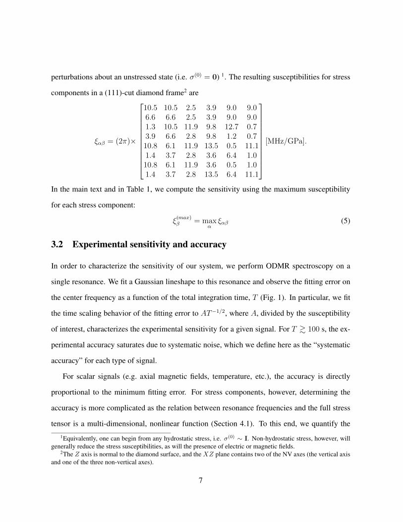
perturbations about an unstressed state (i.e. σ(0) = 0) 1. The resulting susceptibilities for stress

components in a (111)-cut diamond frame2 are

ξαβ = (2π)×

10.5 10.5 2.5 3.9 9.0 9.06.6 6.6 2.5 3.9 9.0 9.01.3 10.5 11.9 9.8 12.7 0.73.9 6.6 2.8 9.8 1.2 0.710.8 6.1 11.9 13.5 0.5 11.11.4 3.7 2.8 3.6 6.4 1.010.8 6.1 11.9 3.6 0.5 1.01.4 3.7 2.8 13.5 6.4 11.1

[MHz/GPa].

In the main text and in Table 1, we compute the sensitivity using the maximum susceptibility

for each stress component:

ξ(max)β = max

αξαβ (5)

3.2 Experimental sensitivity and accuracy

In order to characterize the sensitivity of our system, we perform ODMR spectroscopy on a

single resonance. We fit a Gaussian lineshape to this resonance and observe the fitting error on

the center frequency as a function of the total integration time, T (Fig. 1). In particular, we fit

the time scaling behavior of the fitting error to AT−1/2, where A, divided by the susceptibility

of interest, characterizes the experimental sensitivity for a given signal. For T & 100 s, the ex-

perimental accuracy saturates due to systematic noise, which we define here as the “systematic

accuracy” for each type of signal.

For scalar signals (e.g. axial magnetic fields, temperature, etc.), the accuracy is directly

proportional to the minimum fitting error. For stress components, however, determining the

accuracy is more complicated as the relation between resonance frequencies and the full stress

tensor is a multi-dimensional, nonlinear function (Section 4.1). To this end, we quantify the

1Equivalently, one can begin from any hydrostatic stress, i.e. σ(0) ∼ I. Non-hydrostatic stress, however, willgenerally reduce the stress susceptibilities, as will the presence of electric or magnetic fields.

2The Z axis is normal to the diamond surface, and the XZ plane contains two of the NV axes (the vertical axisand one of the three non-vertical axes).

7

81

2

4

68

10

Mag

netic

fiel

d ac

cura

cy (µ

T)1

2 4 610

2 4 6100

2

Integration time (s)

0.05

0.1

0.2

0.4 Frequency accuracy (MH

z)

Figure 1: Scaling of magnetic field accuracy as a function of total integration time on a singleresonance. Right axis corresponds to standard deviation of center frequency fitting. Solid linecorresponds to a fit to AT−1/2 where A is the sensitivity reported in the main text and T isthe total integration time. Dashed line corresponds to the scaling predicted by Eq. 1. Theexperimental accuracy saturates for T & 100 s due to systematic noise.

accuracy of each stress component using a Monte Carlo procedure. We begin with an unstressed

state, which corresponds to the initial set of frequencies f (0)α = Dgs. We then apply noise to each

of the freqencies based on the minimum fitting error determined above—i.e. f (0)α + δfα, where

δfα are sampled from a Gaussian distribution with a width of the fitting error—and calculate

the corresponding stress tensor using a least-squared fit (Sec. 4.1). Repeating this procedure

over many noise realizations, we compute the standard deviation of each stress component. The

results of this procedure are shown in Table 1.

3.3 Comparison to other magnetometry techniques

In this section, we discuss the comparison of magnetometry techniques presented in Fig. 1F of

the main text. For each sensor, the corresponding dipole accuracy (as defined in Section 3.2)

is plotted against its relevant “spatial resolution,” roughly defined as the length scale within

which one can localize the source of a magnetic signal. In the following discussion, we specify

the length scale plotted for each method in Fig. 1F of the main text. We consider two broad

8

Signal (unit) Theo Sensitivity Exp Sensitivity Accuracy(unit/

√Hz) (unit/

√Hz) (unit)

Hydrostatic stress (GPa) 0.017 0.023 0.0012Average normal stress (GPa) 0.022 0.03 0.0032Average shear stress (GPa) 0.020 0.027 0.0031

Magnetic field (µT) 8.8 12 2.2Magnetic dipole (emu), 5.5× 10−12 7.5× 10−12 1.4× 10−12

floating sample (d = 5 µm)Magnetic dipole (emu), 1.7× 10−20 2.3× 10−20 4.3× 10−21

exfoliated sample (d = 5 nm)(∗)

Magnetic dipole (emu), 1.6× 10−21 2.2× 10−21 4.0× 10−22

exfoliated sample,single NV (d = 5 nm)(†)

Electric field (kV/cm), 1.8 2.5 0.45single NV(†)

Temperature (K), 0.4 0.55 0.10single NV(†)

Table 1: NV sensitivity and accuracy for various signals. Sensitivity is calculated using Eqs. 2-3. We also report the typical fitting error of the center frequency for the relevant experimentsin the main text. Gray rows correspond to projected sensitivity given an exfoliated sampleatop (∗) an ensemble of 5 nm depth NV centers or (†) a single 5 nm depth NV center with∆ν = 1 MHz, C = 0.1,R = 104 s−1. Magnetic dipoles are reported in units of emu, where 1emu = 10−3 A·m2.

9

categories of high pressure magnetometers.

The first category encompasses inductive methods such as pickup coils (3–5) and super-

conducting quantum interference devices (SQUIDs) (6–10)3. Magnetic dipole measurement

accuracies are readily reported in various studies employing inductive methods. We estimate

the relevant length scale of each implementation as the pickup coil or sample bore diameter.

The second class of magnetometers comprises high energy methods including Mossbauer

spectroscopy (11–13) and x-ray magnetic circular dichroism (XMCD) (14–17), which probe

atomic scale magnetic environments. For the Mossbauer studies considered in our analysis, we

calculate magnetic dipole moment accuracies by converting B-field uncertainties into magnetic

moments, assuming a distance to the dipole on order of the lattice spacing of the sample. We

assess the length scale as either the size of the absorbing sample or the length scale associated

with the sample chamber/culet area. For XMCD studies, we accept the moment accuracies

reported in the text. Length scales are reported as the square root of the spot size area. Notably,

we emphasize that both methods provide information about atomic scale dipole moments rather

than a sample-integrated magnetic moment; these methods are thus not directly comparable to

inductive methods.

We compare these methods alongside the NV center, whose accuracy is defined in Sec-

tion 3.2 and shown in Table 1. For the current work, we estimate a length scale ∼ 5 µm, corre-

sponding to the approximate distance between a sample (suspended in a pressure-transmitting

medium) and the anvil culet. By exfoliating a sample onto the diamond surface, the diffraction-

limit ∼ 600 nm bounds the transverse imaging resolution for ensemble NV centers; this limit

can be further improved for single NV centers via super-resolution techniques (18).

3Under the category of inductive methods, we also include the “designer anvil” which embeds a pickup coildirectly into the diamond anvil.

10

4 Stress tensor

4.1 Overview

In this section, we describe our procedure for reconstructing the full stress tensor using NV

spectroscopy. This technique relies on the fact that the four NV crystallographic orientations

experience different projections of the stress tensor within their local reference frames. In par-

ticular, the full Hamiltonian describing the stress interaction is given by:

HS =∑

i

Πz,iS2z,i + Πx,i

(S2y,i − S2

x,i

)+ Πy,i (Sx,iSy,i + Sy,iSx,i) (6)

where

Πz,i = α1

(σ(i)xx + σ(i)

yy

)+ β1σ

(i)zz (7)

Πx,i = α2

(σ(i)yy − σ(i)

xx

)+ β2

(2σ(i)

xz

)(8)

Πy,i = α2

(2σ(i)

xy

)+ β2

(2σ(i)

yz

)(9)

σ(i) is the stress tensor in the local frame of each of NV orientations labeled by i = 1, 2, 3, 4,

and α1,2, β1,2 are stress susceptibility parameters (Section 4.3.3). Diagonalizing this Hamil-

tonian, one finds that the energy levels of each NV orientation exhibit two distinct effects: the

|ms = ±1〉 states are shifted in energy by Πz,i and split by 2Π⊥,i = 2√

Π2x,i + Π2

y,i. Thus, the

Hamiltonian can be thought of as a function that maps the stress tensor in the lab frame to eight

observables: HS(σ(lab)) = Πz,1,Π⊥,1,Πz,2,Π⊥,2, .... Obtaining these observables through

spectroscopy, one can numerically invert this function and solve for all six components of the

corresponding stress tensor.

In practice, resolving the resonances of the four NV orientation groups is not straightforward

because the ensemble spectra can exhibit near degeneracies. When performing ensemble NV

magnetometry, a common approach is to spectroscopically separate the resonances using an

external bias magnetic field. However, unlike magnetic contributions to the Hamiltonian, stress

11

that couples via Π⊥ is suppressed by an axial magnetic field. Therefore, a generic magnetic

field provides only stress information via the shifting parameters, Πz,i, which is insufficient for

reconstructing the full tensor.

To address this issue, we demonstrate a novel technique that consists of applying a well-

controlled external magnetic field perpendicular to each of the NV orientations. This technique

leverages the symmetry of the NV center, which suppresses its sensitivity to transverse magnetic

fields. In particular, for each perpendicular field choice, three of the four NV orientations exhibit

a strong Zeeman splitting proportional to the projection of the external magnetic field along

their symmetry axes, while the fourth (perpendicular) orientation is essentially unperturbed 4.

This enables one to resolve Πz,i for all four orientations and Π⊥,i for the orientation that is

perpendicular to the field. Repeating this procedure for each NV orientation, one can obtain the

remaining splitting parameters and thus reconstruct the full stress tensor.

In the following sections, we provide additional details regarding our experimental proce-

dure and analysis. In Section 4.2, we describe how to use the four NV orientations to calibrate

three-dimensional magnetic coils and to determine the crystal frame relative to the lab frame.

In Section 4.3, we discuss our fitting procedure, the role of the NV’s local charge environment,

and the origin of the stress susceptibility parameters. In Section 4.4, we present the results of

our stress reconstruction procedure for both (111)- and (110)-cut diamond. In Section 4.5, we

compare our experimental results to finite element simulations.

4A transverse magnetic field leads to shifting and splitting at second order in field strength. We account for theformer through a correction described in Section 4.3, while the latter effect is small enough to be neglected. Morespecifically, the effective splitting caused by magnetic fields is (γBB⊥)2/Dgs ≈ 5 − 10 MHz, which is smallerthan the typical splitting observed at zero field.

12

4.2 Experimental details4.2.1 Electromagnet calibration procedure

To apply carefully aligned magnetic fields, we utilize a set of three electromagnets that are

approximately spatially orthogonal with one another and can be controlled independently via

the application of current. Each coil is placed >10 cm away from the sample to reduce the

magnetic gradient across the (200 µm)2 culet area 5.

To calibrate the magnetic field at the location of the sample, we assume that the field pro-

duced by each coil is linearly porportional to the applied current, I . Our goal is then to find the

set of coefficients, amn such that

Bm =∑

m

amnIn, (10)

where Bm = BX , BY , BZ is the magnetic field in the crystal frame and n = 1, 2, 3 indexes

the three electromagnets. We note that this construction does not require the electromagnets to

be spatially orthogonal.

To determine the nine coefficients, we apply arbitrary currents and measure the Zeeman

splitting of the four NV orientations via ODMR spectroscopy. Notably, this requires the abil-

ity to accurately assign each pair of resonances to their NV crystallographic orientation. We

achieve this by considering the amplitudes of the four pairs of resonances, which are pro-

portional to the relative angles between the polarization of the excitation laser and the four

crystallagraphic orientations. In particular, the |ms = 0〉 ↔ |ms = ±1〉 transition is driven by

the perpendicular component of the laser field polarization with respect to the NV’s symmetry

axis. Therefore, tuning the laser polarization allows us to assign each pair of resonances to a

particular NV orientation.

In order to minimize the number of fitting variables, we choose magnetic fields whose pro-

jection along each NV orientation is sufficient to suppress their transverse stress-induced energy5We note that the pressure cell, pressure medium and gasket are nonmagnetic.

13

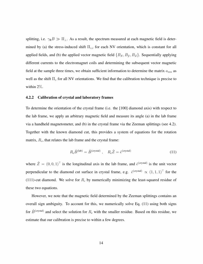
splitting, i.e. γBB Π⊥. As a result, the spectrum measured at each magnetic field is deter-

mined by (a) the stress-induced shift Πz,i for each NV orientation, which is constant for all

applied fields, and (b) the applied vector magnetic field BX , BY , BZ. Sequentially applying

different currents to the electromagnet coils and determining the subsequent vector magnetic

field at the sample three times, we obtain sufficient information to determine the matrix amn as

well as the shift Πz for all NV orientations. We find that the calibration technique is precise to

within 2%.

4.2.2 Calibration of crystal and laboratory frames

To determine the orientation of the crystal frame (i.e. the [100] diamond axis) with respect to

the lab frame, we apply an arbitrary magnetic field and measure its angle (a) in the lab frame

via a handheld magnetometer, and (b) in the crystal frame via the Zeeman splittings (see 4.2).

Together with the known diamond cut, this provides a system of equations for the rotation

matrix, Rc, that relates the lab frame and the crystal frame:

RcB(lab) = B(crystal) , RcZ = e(crystal) (11)

where Z = (0, 0, 1)> is the longitudinal axis in the lab frame, and e(crystal) is the unit vector

perpendicular to the diamond cut surface in crystal frame, e.g. e(crystal) ∝ (1, 1, 1)> for the

(111)-cut diamond. We solve for Rc by numerically minimizing the least-squared residue of

these two equations.

However, we note that the magnetic field determined by the Zeeman splittings contains an

overall sign ambiguity. To account for this, we numerically solve Eq. (11) using both signs

for B(crystal) and select the solution for Rc with the smaller residue. Based on this residue, we

estimate that our calibration is precise to within a few degrees.

14

4.3 Analysis4.3.1 Extracting splitting and shifting information

Having developed a technique to spectrally resolve the resonances, we fit the resulting spectra

to four pairs of Lorentzian lineshapes. Each pair of Lorentzians is defined by a center frequency,

a splitting, and a common amplitude and width. To sweep across the two-dimensional layer of

implanted NV centers, we sequentially fit the spectrum at each point by seeding with the best-fit

parameters of nearby points. We ensure the accuracy of the fits by inspecting the frequencies of

each resonance across linecuts of the 2D data (Fig. 2B).

Converting the fitted energies to shifting (Πz,i) and splitting parameters (Π⊥,i) requires us to

take into account two additional effects. First, in the case of the shifting parameter, we subtract

off the second-order shifting induced by transverse magnetic fields. In particular, the effective

shifting is given by Πz,B ≈ (γBB⊥)2/Dgs, which, under our experimental conditions, corre-

sponds to Πz,B ≈ 5 − 10 MHz. To characterize this shift, one can measure each of the NV

orientations with a magnetic field aligned parallel to its principal axis, such that the transverse

magnetic shift vanishes. In practice, we obtain the zero-field shifting for each of the NV orien-

tations without the need for additional measurements, as part of our electromagnet calibration

scheme (Section 4.2). We perform this calibration at a single point in the two-dimensional map

and use this point to characterize and subtract off the magnetic-induced shift in subsequent mea-

surements with arbitrary applied field. Second, in the case of the splitting parameter, we correct

for an effect arising from the NV’s charge environment. We discuss this effect in the following

section. The final results for the shifting (Πz,i) and splitting (Π⊥,i) parameters for the (111)-cut

diamond at 4.9 GPa are shown in Fig. 2C.

15

A B

C

MHz MHz MHz

MHzMHzMHz

M M

50 μm

Figure 2: Stress reconstruction procedure applied to the (111)-cut diamond at 4.9 GPa. (A) Atypical ODMR spectrum with the resonances corresponding to each NV orientation fit a pair ofLorentzian lineshapes. (B) A linecut indicating the fitted resonance energies (colored points)superimposed on the measured spectra (grey colormap). (C) 2D maps of the shifting (Πz,i) andsplitting parameters (Π⊥,i) for each NV orientation across the entire culet.

16

4.3.2 Effect of local charge environment

It is routinely observed that ensemble spectra of high-density samples (i.e. Type 1b) exhibit a

large (5 − 10 MHz) splitting even under ambient conditions. While commonly attributed to

instrinsic stresses in the diamond, it has since been suggested that the splitting is, in fact, due to

electric fields originating from nearby charges (19). This effect should be subtracted from the

total splitting to determine the stress-induced splitting.

To this end, let us first recall the NV interaction with transverse electric fields:

HE = d⊥[Ex(S2

y − S2x) + Ex(SxSy + SySx)

](12)

where d⊥ = 17 Hz cm/V. Observing the similarity with Eq. (6), we can define

Πx = Πs,x + ΠE,x (13)

Πy = Πs,y + ΠE,y (14)

where ΠS,x,y are defined in Eq. (7) and ΠE,x,y = d⊥Ex,y. The combined splitting for

electric fields and stress is then given by

2Π⊥ = 2((Πs,x + ΠE,x)

2 + (Πs,y + ΠE,y)2)1/2

. (15)

We note that the NV center also couples to longitudinal fields, but its susceptibility is ∼ 50

times weaker and is thus negligible in the present context.

To model the charge environment, we consider a distribution of transverse electric fields.

For simplicity, we assume that the electric field strength is given by a single value E0, and its

angle is randomly sampled in the perpendicular plane. Adding the contributions from stress and

17

electric fields and averaging over angles, the total splitting becomes

Π⊥,avg =

∫dθ(Π2

S,⊥ + Π2E,⊥ + 2ΠS,⊥ΠE,⊥ cos θ)1/2

=1

π

√

Π2s,⊥ − Π2

E,⊥EllipticE

− 4ΠS,⊥ΠE,⊥√

Π2S,⊥ − Π2

E,⊥

+√

Π2S,⊥ + Π2

E,⊥EllipticE

− 4Πs,⊥ΠE,⊥√

Π2S,⊥ + Π2

E,⊥

(16)

where EllipticE(z) is the elliptic integral of the second kind. This function is plotted in Fig. 3A,

and we note its qualitative similarity to a quadrature sum.

To characterize the intrinsic charge splitting (ΠE,⊥), we first aquire an ODMR spectrum for

each diamond sample under ambient conditions. For example, for the (111)-cut diamond, we

measured ΠE,⊥ ≈ 4.5 MHz. For subsequent measures under pressure, we then subtract off

the charge contribution from the observed splitting by numerically from inverting Eq. (16) and

solving for Πs,⊥.

4.3.3 Susceptibility parameters

A recent calibration experiment established the four stress susceptibilities relevant to this work

(20). In this section, we discuss the conversion of their susceptibilities to our choice of basis

(the local NV frame), and we reinterpret their results for the splitting parameters taking into

account the effect of charge.

In their paper, Barson et. al. define the stress susceptilities with respect diamond crystal

frame:

Πz = a1(σXX + σYY + σZZ) + 2a2(σYZ + σZX + σXY) (17)

Πx = b(2σZZ − σXX − σYY) + c(2σXY − σYZ − σZX ) (18)

Πy =√

3 [b(σXX − σYY) + c(σYZ − σZX )] (19)

18

whereXYZ are the principal axes of the crystal frame. Their reported results are a1, a2, b, c =

(2π)× 4.86(2),−3.7(2), 2.3(3), 3.5(3)MHz/GPa.

To convert these susceptibilities to our notation (Eq. 6), one must rotate the stress tensor

from the crystal frame to the NV frame, i.e. σxyz = RσXYZR>. The rotation matrix that

accomplishes this is:

R =

− 1√

6− 1√

6

√23

1√2− 1√

20

1√3

1√3

1√3

. (20)

Applying this rotation, one finds that the above equations become (in the NV frame)

Πz = (a1 − a2)(σxx + σyy) + (a1 + 2a2)σzz (21)

Πx = (−b− c)(σyy − σxx) + (√

2b−√

2

2c)(2σxz) (22)

Πx = (−b− c)(2σxy) + (√

2b−√

2

2c)(2σyz) (23)

Thus, the conversion between the two notations is(α1

β1

)=

(1 −11 2

)(a1

a2

)

(α2

β2

)=

(−1 −1√2 −

√2

2

)(bc

) (24)

In characterizing the splitting parameters (b and c), Barson et. al. assumed a linear depen-

dence between the observed splitting and ΠS,⊥. However, our charge model suggests that for

ΠS,⊥ . ΠE,⊥ the dependence should be nonlinear. To account for this, we re-analyze their data

using Eq. 16 as our fitting form, rather than a linear function as in the original work. The results

are shown in Fig. 3 for two NV orientation groups measured in the experiment: (110)36 and

(100)54, where (· · · ) denotes the crystal cut and the subscript is the angle of the NV group with

respect to the crystal surface. From the fits, we extract the linear response, Πs,⊥/P , for the two

groups. These are related to the stress parameters by b − c and 2b, respectively. Using these

19

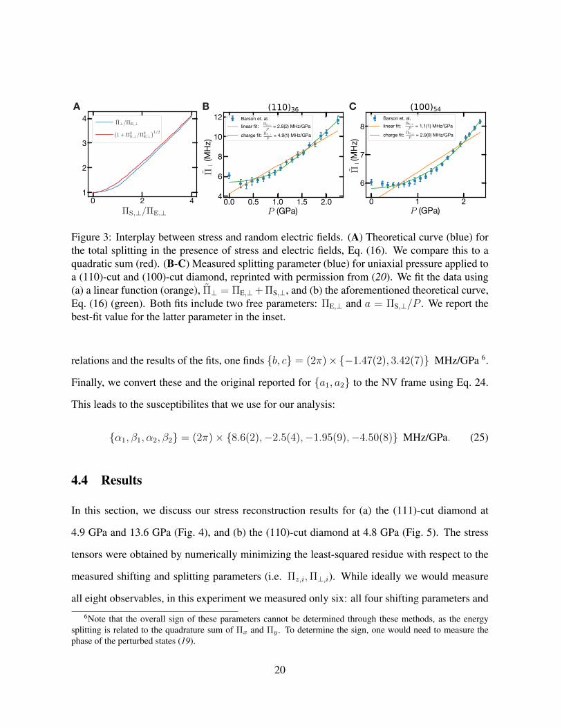
A B C

Figure 3: Interplay between stress and random electric fields. (A) Theoretical curve (blue) forthe total splitting in the presence of stress and electric fields, Eq. (16). We compare this to aquadratic sum (red). (B-C) Measured splitting parameter (blue) for uniaxial pressure applied toa (110)-cut and (100)-cut diamond, reprinted with permission from (20). We fit the data using(a) a linear function (orange), Π⊥ = ΠE,⊥+ ΠS,⊥, and (b) the aforementioned theoretical curve,Eq. (16) (green). Both fits include two free parameters: ΠE,⊥ and a = ΠS,⊥/P . We report thebest-fit value for the latter parameter in the inset.

relations and the results of the fits, one finds b, c = (2π)×−1.47(2), 3.42(7) MHz/GPa 6.

Finally, we convert these and the original reported for a1, a2 to the NV frame using Eq. 24.

This leads to the susceptibilites that we use for our analysis:

α1, β1, α2, β2 = (2π)× 8.6(2),−2.5(4),−1.95(9),−4.50(8) MHz/GPa. (25)

4.4 Results

In this section, we discuss our stress reconstruction results for (a) the (111)-cut diamond at

4.9 GPa and 13.6 GPa (Fig. 4), and (b) the (110)-cut diamond at 4.8 GPa (Fig. 5). The stress

tensors were obtained by numerically minimizing the least-squared residue with respect to the

measured shifting and splitting parameters (i.e. Πz,i,Π⊥,i). While ideally we would measure

all eight observables, in this experiment we measured only six: all four shifting parameters and

6Note that the overall sign of these parameters cannot be determined through these methods, as the energysplitting is related to the quadrature sum of Πx and Πy . To determine the sign, one would need to measure thephase of the perturbed states (19).

20

two splitting parameters. We find that this information allows for the robust characterization of

σZZ and σ⊥ = 12(σXX + σY Y ), i.e. the two azimuthally symmetric normal components.

We can estimate the accuracy of the reconstructed tensors from the spatial variations of

σZZ at 4.9 GPa. Assuming the medium is an ideal fluid, one would expect that σZZ to be flat

in the region above the gasket hole. In practice, we observe spatial fluctuations characterized

by a standard deviation ≈ 0.01 GPa; this is consistent with the expected accuracy based on

frequency noise (Table 1). The errorbars in the reconstructed stress tensor are estimated using

the aforementioned experimental accuracy.

Interestingly, the measured values for σZZ differs from the ruby pressure scale by ∼ 10%.

This discrepancy is likely explained by inaccuracies in the susceptibility parameters; in particu-

lar, the reported susceptibility to axial strain (i.e. β1) contains an error bound that is also∼ 10%.

Other potential sources of systematic error include inaccuracies in our calibration scheme or the

presence of plastic deformation.

Finally, we note that, in many cases, our reconstruction procedure yielded two degenerate

solutions for the non-symmetric stress components; that is, while σZZ and σ⊥ have a unique

solution, we find two different distributions for σXX , σXY , etc. This degeneracy arises from the

squared term in the splitting parameter, Π⊥,i = 2√

Π2x,i + Π2

y,i, and the fact we measure only

six of the eight observables. In Fig. 4 and Fig. 5 (and Fig. 2B of the main text), we show the

solution for the stress tensor that is more azymuthally symmetric, as physically motivated by

our geometry.

4.5 Finite element simulations of the stress tensor

Using equations from elasticity theory under the finite element approach, a numerical simula-

tion was coded in ABAQUS for the stress and strain tensor fields in the diamond anvil cell.

The diamond anvil cell is approximately axially symmetric about the diamond loading axis, in

21

GPa GPa GPa

GPaGPaGPa

GPa GPa GPa

GPaGPaGPa

A

B

Figure 4: Stress tensor reconstruction of (111)-cut diamond at (A) 4.9 GPa and (B) 13.6 GPa.In the former case, we reconstruct both the inner region in contact with the fluid-transmittingmedium, and the outer region in contact with the gasket. In the latter case, we reconstruct onlythe inner region owing to the large stress gradients at the contact with the gasket; note that theblack pixels in the center indicates where the spectra is obscured by the ruby flourescence. Asdescribed in the main text, both pressures exhibit inward concentration of the normal lateralstress (σXX and σY Y ). In contrast, the normal loading stress is uniform for the lower pressureand spatially varying at the higher pressure, indicating that the pressure medium has solidified.

22

GPa GPa GPa

GPaGPaGPa

50 μm

Figure 5: Stress tensor reconstruction of (110)-cut diamond at 4.8 GPa pressure. Analogous tothe (111)-cut at low pressure, we observe an inward concentration of lateral stress and a uniformloading stress in the fluid-contact region.

23

Figure 6: (A) Diamond geometry, (B) anvil tip with distribution of the applied normal stress,(C) distribution of the applied shear stress. Normal stress σZZ at the culet and zero shear stressσRZ along the pressure-transmitting medium/anvil boundary (r ≤ 47 µm) are taken from exper-iment. Normal and shear contact stresses along all other contact surfaces are determined fromthe best fit of the mean in-plane stress distribution σ⊥ = 0.5(σRR + σΘΘ) to experiment (maintext Fig. 2A and Fig. 7)

this case the crytallographic (111) axis (i.e. the Z axis). This permits us to improve simulation

efficiency by reducing the initially 3D tensor of elastic moduli to the 2D axisymmetric cylin-

drical frame of the diamond as follows. Initially, the tensor can be written in 3D with cubic

axes c11 = 1076 GPa, c12 = 125 GPa, c44 = 577 GPa. Next, we rotate cubic axes such that the

(111) direction is along the Z axis of the cylindrical coordinate system. Finally, the coordinate

system is rotated by angle θ around the Z axis and the elastic constants are averaged over 360

rotation. The resulting elasticity tensor in the cylindrical coordinate system is

1177.5 57.4 91 057.4 1211.6 57.4 091 57.4 1177.5 00 0 0 509.2

[GPa].

The geometry of the anvil and boundary conditions (Fig. 6) are as follows:

1. The top surface of the anvil is assumed to be fixed. The distribution of stresses or dis-

24

placements along this surface does not affect our solution close to the diamond culet line

AB.

2. The normal stress σZZ along the line AB is taken from the experimental measurements

(main text Fig. 2A and 7). The pressure-transmitting medium/gasket boundary runs

along the innermost 47 µm of this radius.

3. Along the pressure-transmitting medium/anvil boundary (r ≤ 47 µm) and also at the

symmetry axis r = 0 (line AE) shear stress σRZ is zero. Horizontal displacements at the

symmetry axis are also zero.

4. Normal and shear contact stresses along all other contact surfaces are determined from

the best fit to the mean in-plane stress distribution σ⊥ = 0.5(σRR + σΘΘ) measured in

the experiment (main text Fig. 2A and Fig. 7 ). We chose to fit to σ⊥ rather than to other

measured stresses is because it has the smallest noise in experiment. With this, the normal

stress on the line BD with the origin at point B is found to be

σc = 3.3× 105x4 − 7.5× 104x3 + 4.5× 103x2 − 102x+ 4.1, (26)

where σc is in units of GPa, and the position x along the lateral side is in units of mm.

The distribution of the normal stresses is shown in Fig. 6B and Fig. 8.

5. At the contact surface between the gasket and the anvil, a Coulomb friction model is

applied. The friction coefficient on the culet is found to be 0.02 and along the inclined

surface of the anvil (line BD) is found to vary from 0.15 at point B to 0.3 at 80 µm from

the culet. The distribution of shear stresses is shown in Fig. 6C and Fig. 8.

6. Other surfaces not mentioned above are stress-free.

The calculated distributions of the stress tensor components near the tip of the anvil are

shown in Fig. 9.

25

(A) (B)

Figure 7: (A) Distribution of applied normal stress σZZ and the mean in-plane stress σ⊥ alongthe culet surface of the diamond from the experiment and FEM simulations. (B) Distribution ofthe mean in-plane stress σ⊥ (experimental and simulated) as well as the simulated radial σRRand circumferential σΘΘ stresses along the culet surface of the diamond.

Figure 8: Distribution of applied normal and shear stress along the lateral surface of the diamonddetermined from the best fit of the mean in-plane stress distribution σ⊥ to experiment (main textFig. 2A and Fig. 7).

5 Iron dipole reconstruction

In this section, we discuss the study of the pressure-induced α ↔ ε transition in iron. In

particular, we provide the experimental details, describe the model used for fitting the data, and

26

Figure 9: Calculated distributions of the components of stress tensor in the anvil for r < 150and z < 475 µm.

outline the procedure to ascertain the transition pressure.

For this experiment, the DAC is prepared with a rhenium gasket preindented to 60 µm

thickness and laser drilled with a 100 µm diameter hole. We load a ∼ 10 µm iron pellet,

extracted from a powder (Alfa Aesar Stock No. 00737-30), and a ruby microsphere for pres-

sure calibration. A solution of methanol, ethanol and water (16:3:1 by volume) is used as the

pressure-transmitting medium.

The focused laser is sequentially scanned across a 10×10 grid corresponding to a ∼ 30 ×

30 µm area of the NV layer in the vicinity of the iron pellet, taking an ODMR spectrum at each

point. As discussed in the main text, the energy levels of the NV are determined by both the

magnetic field and the stress in the diamond. Owing to their different crystallographic orienta-

tions, the four NV orientations in general respond differently to these two local parameters. As

a result, for each location in the scan, eight resonances are observed.

A large bias magnetic field (∼ 180 G), not perpendicular to any of the axes, is used to

suppress the effect of the transverse stress in the splitting for each NV orientation. However,

the longitudinal stress still induces an orientation-dependent shift of the resonances which is

27

Figure 10: (A) Example of a typical spectrum with a fit to eight free Gaussians. Resonance pairsare identified as in Fig. 1D of the main text: NV4 has the strongest magnetic field projection andNV1 has the weakest. (B) Example spectrum for which resonances are broadened and shifted.In this case we cannot correlate any resonances in the spectrum to specific NV orientations.

nearly constant across the imaging area, as measured independently (Fig 2C).

By analyzing the splittings of the NV resonances across the culet, we can determine the

local magnetic field and thereby reconstruct the dipole moment of the iron pellet.

To estimate the error in pressure, a ruby fluorescence spectrum was measured before and

after the ODMR mapping, from which the pressure could be obtained (21). The pressure was

taken to be the mean value, while the error was estimated using both the pressure range and the

uncertainty associated with each pressure point.

5.1 Extracting Splitting Information

The eight resonances in a typical ODMR spectrum are fit to Gaussian lineshapes to extract the

resonance frequency (Fig 10A). Resonances are paired as in Fig. 1D of the main text: from

outermost resonances to innermost, corresponding to NV orientations with the strongest mag-

netic field projection to the weakest, respectively. Once identified, we calculate the splitting and

magnetic field projection for each NV orientation.

28

We note that there are two regimes where our spectra cannot confidently resolve and identify

all the eight resonances. First, at high pressure, the resonance contrast for some NV orienta-

tions is diminished, possibly due to a modification of the frequency response of the microwave

delivery system. Second, close to or on top of the iron pellet, the resonances are broadened; we

attribute this to the large magnetic field gradients (relative to the imaging resolution) caused by

the sample. The resulting overlap in spectral features obfuscates the identity of each resonance

(Fig. 10B). In both cases, we fit and extract splittings only for the orientations we could identify

with certainty.

5.2 Point Dipole Model

We model the magnetization of our pellet sample as a point dipole at some location within the

sample chamber. The total magnetic field is then characterized by the external applied field,

B0, the dipole of the sample, d, and the position of the dipole, r. Because of the presence of a

large applied field, we observe that the magnetization of the sample aligns with B0, and thus,

we require only the strength of the dipole to characterize its moment, d = DB0. We expect

the external magnetic field and the depth of the particle to remain nearly constant at different

pressures. This is indeed borne out by the data, see Sec. 5.4. As a result, we consider the external

magnetic field B0 = (−23(7),−160(1), 92(2)) G and depth of the iron pellet rZ = −5(1) µm

to be fixed.

Due to the dipole of the iron pellet, the magnetic field across the NV layer at position x is

given by:

B(x) = B0 +µ0

4π

1

|x|3 (3x(d · x)− d) , (27)

where hats represent unit vectors. At each point, the local field induces a different splitting,

∆(i), to the 4 NV crytallographic orientations i ∈ 1, 2, 3, 4, measured by diagonalizing the

Hamiltonian H = DgsS2z +B

(i)z Sz +B

(i)⊥ Sx, where Bz = |B · z(i)| is the projection of B onto

29

the axis of the NV, and B(i)⊥ =

√|B|2 − (B

(i)z )2, its transverse component. Dgs is the zero

field splitting of the NV. For each choice of D, rX and rY , we obtain a two dimensional map of

∆(i). Performing a least squares fit of this map against the experimental splittings determines

the best parameters for each pressure point. The error in the fitting procedure is taken as the

error in the dipole strength D.

5.3 Determining Transition Pressure

Although the α ↔ ε structural phase transition in iron is a first order phase transition, we do

not observe a sharp change in the dipole moment of the sample, observing instead a cross-over

between the two magnetic behaviors. We attribute this to the non-hydrostatic behavior of the

sample chamber at high pressures. As a result, different parts of the iron pellet can experience

different amounts of pressure and, thus, undergo a phase transition at different applied pressures.

The measured dipole moment should scale with the proportion of the sample that has undergone

the phase transition. This proportion, p(P ), should plateau at either 0 or 1 on different sides

of the phase transition, and vary smoothly across it. To model this behavior we use a logistic

function:

p(P ) =1

eB(P−Pc) + 1. (28)

The dipole strength is then given by:

D = p(P )Dα + [1− p(P )]Dε , (29)

where Dα (Dε) is the dipole moment of the sample in the α (ε) structural phase and 1/B

corresponds to the width of the transition, thus its uncertainty.

5.3.1 Large error bar in the 11 GPa decompression point

During the decompression, around 11 GPa, we observed a significant drift of the pressure dur-

ing measurement of the ODMR spectra. Unfortunately, the starting pressure was close to the

30

Data Reconstructed

800

900

1000

MH

z

10 µm

Figure 11: Measured map of the splittings of one of the NV orientations (left). Near the top ofthe plot we observe a much stronger splitting compared to the bottom of the plot. Throughoutthe measurement, the shift in the pressure induced a shift in the dipole moment of the sample.We consider 3 different regions (seperated by horizontal lines) corresponding to 3 differentdipole strengths. The reconstructed map of the splittings is shown on the right in agreementwith the data. From the center and the spread of dipole strengths, we extract the dipole momentand its error. Black bar corresponds to 10 µm.

transition pressure, and the drift in pressure led to a very large change in the pellet’s dipole mo-

ment throughout the scanning measurement. This is clear in the measured data, Fig. 11, with

the top-half of the map displaying a significantly larger shift with respect to the bottom-half.

To extract the drift in the dipole moment, we divide the two-dimensional map into three

different regions, each assumed to arise from a constant value of the dipole moment of the

pellet. By fitting to three different dipole moments (given a fixed position, rX and rY ) we

obtain an estimate of the drift of the dipole moment that allows us to compute an errorbar of that

measurement. The estimated dipole moment at this pressure point is taken as the midpoint of the

three extracted values,Dmax +Dmin

2, while the error is estimated by the range,

Dmax −Dmin

2.

5.4 Fitting to external magnetic field and depth

In this section we present additional data where we have allowed both the external magnetic

field and the depth of the iron pellet to vary in the fitting procedure. The result of the fitting

procedure is summarized in Fig. 12.

31

In particular, we expect the external magnetic field and the depth of the pellet to remain

constant at different pressures. Indeed, we observe this trend in the extracted parameters,

Fig. 12(A,B). Using the mean and standard deviation, we estimate these values and their er-

rors, quoted in Sec. 5.2. The final fitting procedure with these values fixed is presented in the

main text.

6 Gadolinium

6.1 Experimental detail

We use a custom-built closed cycle cryostat (Attocube attoDRY800) to study the P -T phase

diagram of Gd. The DAC is placed on the sample mount of the cryostat, which is incorporated

with a heater and a temperature sensor for temperature control and readout.

For this experiment, we use beryllium copper gaskets. The Gd sample is cut from a 25 µm

thick Gd foil (Alfa Aesar Stock No. 12397-FF) to a size of ∼ 30µm × 30µm and loaded with

cesium iodide (CsI) as the pressure-transmitting medium. A single ruby microsphere loaded

into the chamber is used as a pressure scale.

For each experimental run, we start with an initial pressure (applied at room temperature

300 K) and cool the cell in the cryostat. Due to contraction of the DAC components with

decreasing temperature, each run of the experiment traverses a non-isobaric path in P -T phase

space, Fig. 14A. Using fiducial markers in the confocal scans of the sample chamber, we track

points near and far from the Gd sample throughout the measurement. By performing ODMR

spectroscopy at these points for each temperature, we monitor the magnetic behavior of the

sample. More specifically, comparing the spectra between the close point (probe) against the

far away one (control), Fig. 13, enables us to isolate the induced field from the Gd sample.

32

10 20Pressure (GPa)

100

0

100

200

Mag

netic

Fie

ld (G

)

10 20Pressure (GPa)

10

0

10

20

30

Pos

ition

(m

)

A

C

B

5 10 15 20Pressure (GPa)

10 10

10 9

10 8

Dip

ole

Str

engt

h (e

mu)

-Iron

-Iron

CompressionDecompression

BX BY BZ B0 rX rY rZ

Figure 12: Result of fitting procedure when the external magnetic field and the depth of theiron pellet is allowed to vary at each pressure. (A)[(B)] External magnetic field [position of thepellet] extracted as a function of pressure (circles correspond to compression while diamondscorrespond to decompression). Across the entire range of pressures, the extracted externalmagnetic field and the depth of the iron pellet is approximately constant. In the final fitting pro-cedure, these values are fixed to their extracted mean (dashed lines). Shaded regions correspondto a standard deviation above and below the mean value. (C) Dipole strength of the iron pel-let, extracted when all seven parameters (BX , BY , BZ , D, rX , rY , rZ) are fitted. The resultingtransitions occur at 17.2 GPa and 10.8 GPa for compression and decompression, respectively.Comparing with the width of the transition (1.3 GPa), these values are in excellent agreementwith those presented in the main text.

33

A B

Probe

Controlruby

Gd

Figure 13: (A) The protocol for obtaining P -T phase map of Gd relies on monitoring theODMR spectrum versus temperature and pressure at a point of interest (probe) near the sample.To verify that the observed signal is from the Gd flake, one can perform the same measurementon a control point further away from the sample. (B) The difference in the splitting between theprobe and control points isolates the magnetic field generated by the Gd sample, allowing us tomonitor the magnetic behavior of the sample.

6.2 Fitting phase transition

There are three different transitions we which to locate in the study of the Gd’s P -T phase

diagram: a magnetic transition from PM dhcp to FM dchp; structural phase transitions, either

hcp→ dhcp or Sm-type↔ dhcp; and a magnetic phase transition from PM Sm-type to AFM

Sm-type.

In order to extract the transition temperature of the paramagnet to ferromagnet transition

from our data, we model the magnetization of our sample near the magnetic phase transition

using a regularized mean field theory.

The magnetism of gadolinium is well-described by a three dimensional Heisenberg magnet

of core electrons (22). In the presence of an external magnetic field, the free energy near the

critical point is expanded in even powers of the magnetization with a linear term that couples to

the external magnetic field:

f = −Bm+α

2(T − TC)m2 +

β

4m4, (30)

34

where m is the magnetization, B is the external magnetic field, α and β the expansion coef-

ficients, T the temperature, and TC the transition temperature. In this treatment, we implicitly

assume that α and β do not vary significantly with pressure and thus can be taken to be constant

across paths in P -T phase space. The magnetization mmin is then obtained by minimizing the

free energy.

Because our observation region extends far away from the transition, we observe a plateau-

ing of the splittings that emerges from the microscopics of Gd. Using R as the regularization

scale and A as the maximum magnetization of the sample we propose the simple regularization

scheme:

m(T, P ) = Ammin

mmin +R. (31)

The splitting of the NV group, up to some offset, is proportional to the magnetization of

the sample. This proportionality constant, A, captures he relation between magnetization and

induced magnetic field, the geometry of sample relative to the measurement spot, as well as the

susceptibility of the NV to the magnetic field. The splitting of the NV is then given by:

∆ = Ammin

mmin +R+ c (32)

where we incorporated A into A as well. Normalizing α and β with respect to B, we obtain six

parameters that describe the magnetization profile, directly extracting TC.

In the case of the first order structural phase transitions, similar to that of iron, we take the

susceptibility to follow a logistic distribution. We model the observed splitting as:

∆ =A

eB(T−TC) + 1+ c (33)

Fitting to the functional form provides the transition temperature TC. Error bar is taken as largest

between 1/B and the fitting error.

In the case of the paramagnetic to antiferromagnetic transition, we use the mean field sus-

ceptibility across the phase transition of the system. The susceptibility across such transition is

35

peaked at the transition temperature:

χ(T ) ∝

1

T − θpT > Tc

C3L′(H/T )

T − θp3L′(H/T )T < Tc

(34)

where C is chosen to ensure continuity of χ, L′(x) is the derivative of the Langevin function

L(x)at, H is a meaasure of the applied field, and θp is the assymptotic Curie point. Finally, we

fit the observed splitting to:

∆ = Aχ(T ;Tc, H, θp) + c (35)

where, as before, A captures both the geometric effects, as well as the response of the chosen

NV group to the magnetic field.

6.3 Additional data

In this section we present the data for the different paths taken in P -T phase and the resulting

fits. Table 2 summarizes the observations for all experimental runs. Fig. 14 contains the data

used in determining the linear pressure dependence of the hcp phase. Fig. 15 comprises the

data used in determining the transition to the dhcp phase, either via the FM hcp to PM dhcp

transition, Fig. 15B, or via the difference in susceptibilities between PM Sm-type and PM dhcp

of Gd, Fig. 15C and D. We emphasize that in the blue path, we begin the experiment below

2 GPa and thus in the hcp structure, while for the orange and green, we begin above 2 GPa, so

we expect the system to be in Sm-type. Finally, Fig. 16 contains the data where we observe a

change in the susceptibility of Gd that occurs at the purported Sm-type PM to AFM transition.

6.4 Recreating the P -T phase diagram of Gd

The rich magnetic behavior of Gd is partially dependent on its structural phases, captured in

the sequence: hexagonal closed packed (hcp) to Samarium (Sm) type at ∼ 2 GPa, and then to

36

280 300 320Temperature (K)

600

620

640

660

NV

Sp

littin

g (M

Hz)

260 280 300 320Temperature (K)

620

640

NV

Sp

littin

g (M

Hz)

260 280 300 320Temperature (K)

600

650

700

750

NV

Sp

littin

g (M

Hz)

260 280 300 320Temperature (K)

540

560

580

NV

Sp

littin

g (M

Hz)

260 280 300 320Temperature (K)

540

560

580

NV

Sp

littin

g (M

Hz)

100 200 300Temperature (K)

560

580

600N

V S

plit

ting

(MH

z)

100 200 300Temperature (K)

570

580

590

600

NV

Sp

littin

g (M

Hz)

100 200 300Temperature (K)

580

590

600

NV

Sp

littin

g (M

Hz)

225 250 275 300Temperature (K)

520

540

560

580

NV

Sp

littin

g (M

Hz)

220 240 260 280 300Temperature (K)

520

540

560

580

NV

Sp

littin

g (M

Hz)

220 240 260 280 300Temperature (K)

540

560

580

NV

Sp

littin

g (M

Hz)

225 250 275 300Temperature (K)

50

100

150

200

NV

Sp

littin

g D

iffer

ence

(MH

z)

240 260 280 300Temperature (K)

0

50

100

150

NV

Sp

littin

g D

iffer

ence

(MH

z)

100 200 300Temperature (K)

0

50

100

150

200

NV

Sp

littin

g D

iffer

ence

(MH

z)

0 1 2 3 4 5 6 7 8Pressure (GPa)

0

50

100

150

200

250

300

Tem

per

atur

e (K

)

A

B C D

E F G

H I J

K L M

N O

Figure 14: (A) Paths in the P -T phase space that inform about the hcp PM phase to thehcp FM phase. (B-O) Measured NV splitting and corresponding fit. The resulting transitiontemperatures are highlighted in (A) with squares. Shaded region corresponds to the part of thespectrum fitted. 37

100 200 300Temperature (K)

580

590

600

NV

Sp

littin

g (M

Hz)

150 200 250 300Temperature (K)

585

590

595

600

605

NV

Sp

littin

g (M

Hz)

100 150Temperature (K)

585

590

595

600

605

NV

Sp

littin

g (M

Hz)

0 1 2 3 4 5 6 7 8Pressure (GPa)

0

50

100

150

200

250

300Te

mp

erat

ure

(K)

A

B C D

Figure 15: (A) Paths in the P -T phase space that inform about the transition to the PM dhcpphase. (B-D) Measured NV splitting and corresponding fit. The resulting transition tempera-tures are highlighted in (A) with squares. We interpret (B) as a transition from FM hcp to PMdhcp, while (C),(D) as a transition from PM Sm-type to PM dhcp. Shaded region correspondsto the part of the spectrum fitted.

Temperature (K)

NV

Sp

littin

g (M

Hz)

100 200 300

595

600

605A B

0 1 2 3 4 5 6 7 8Pressure (GPa)

0

50

100

150

200

250

300

Tem

per

atur

e (K

)

Figure 16: (A) Path in the P -T phase space where a signal consistent with the purported AFMtransition in Sm-type Gd is seen (B). Shaded region corresponds to the part of the spectrumfitted.

38

Run Direction Phase transition Remarks, visible in Fig.1 Heat-up hcp (FM) −→ hcp (PM) New sample, Fig. 14B2 Cool-down hcp (PM) −→ hcp (FM) Fig. 14C3 Cool-down hcp (PM) −→ hcp (FM) Fig. 14D4 Cool-down No observation Probably starting in Sm due

to large initial pressure5 Cool-down hcp (PM) −→ hcp (FM) New sample, Fig. 14E6 Heat-up hcp (FM) −→ hcp (PM) Fig. 14F7 Cool-down hcp (PM) −→ hcp (FM) Fig. 14G8 Heat-up hcp (FM) −→ hcp (PM) Fig. 14H9 Cool-down hcp (PM) −→ hcp (FM) Fig. 14I, 15B

−→ dhcp (PM)10 Cool-down Weak evidence for Probably starting in Sm due

Sm (PM) −→ Sm (AFM) to metastability, Fig. 16B11 Cool-down hcp (PM) −→ hcp (FM) New sample, Fig. 14J12 Heat-up hcp (FM) −→ hcp (PM) Fig. 14K13 Cool-down hcp (PM) −→ hcp (FM) Fig. 14L14 Cool-down Weak evidence for Probably starting in Sm due

Sm (PM) −→ dhcp (PM) to large initial pressure15 Cool-down Weak evidence for Probably starting in Sm due

Sm (PM) −→ dhcp (PM) to metastability, Fig. 15C16 Heat-up Weak evidence for Fig. 15D

dhcp (PM) −→ Sm (PM)17 Cool-down hcp (PM) −→ hcp (FM) New sample, Fig. 14M18 Heat-up hcp (FM) −→ hcp (PM) Fig. 14N19 Cool-down hcp (PM) −→ hcp (FM) Fig. 14O

and start of transition to dhcp (PM)

Table 2: Summary of all experimental runs in the P -T phase diagram, indexing either a decreaseor increase in temperature during this path, and the observed phase transitions. Each group ofruns, between double lines in the table, corresponds to a different sample.

39

double hexagonal closed packed (dhcp) at∼ 6 GPa. In particular, while the paramagnetic (PM)

phase of hcp orders to a ferromagnet (FM), the PM phase of Sm-type orders to an antiferromag-

net (AFM) (23). Similarly, dhcp undergoes a PM to magnetically ordered phase transition.

For experimental runs with initial pressures < 2 GPa (runs 1-3, 5-9, 11-13, 17-19), we

observe a PM ↔ FM phase transition in hcp Gd. In agreement with previous studies, we

see a linear decrease of the Curie temperature with increasing pressure up to ∼ 4 GPa (24–

26). Notably, prior studies have shown a structural transition from hcp to Sm-type at 2 GPa

(25, 27, 28), which is believed to be “sluggish” (23, 25). This is indeed consistent with our

observation that the linear dependence of the Curie temperature persists well into the Sm-type

region, suggesting the existence of both structural phases over our experimental timescales.

Furthermore, in run 9 (Table 2 and Fig. 16A,B), we observe a complete loss of FM signal

when pressures exceed ∼ 6 GPa at ∼ 150 K, in good agreement with the previously reported

phase transition from hcp (FM) to dhcp (PM) structure (25,27). Upon performing a similar path

in P -T space (run 19), we observe the same behavior. In contrast to the previous slow hcp to

Sm-type transition, we believe that the equilibrium timescale for the hcp (FM) to dhcp (PM)

transition is much faster at this temperature.

After entering the dhcp structure (run 9), we no longer observe a clear FM signal from the

sample even after heating to 315 K and depressurizing < 0.1 GPa. This can be explained by

the retention of dhcp or Sm-type structure in the sample. Previous studies, suggesting that the

Sm-type phase in Gd is metastable up to ambient pressure and temperature (23), corroborate

that our sample is likely still in the Sm-type structural phase. It is not too surprising, that by

continuing to cool down and walking along a slightly different P -T path, we observe only a

small change in the NV splitting at ∼ 150 K and ∼ 5 GPa as we cross the purported Sm-type

PM to AFM phase boundary (run 10 in Table 2) (23, 25, 27).

Moreover, the metastable dynamics of hcp to Sm-type transitions are strongly pressure and

40

temperature dependent, suggesting that different starting points (in the P -T phase diagram) can

lead to dramatically different behaviors. Indeed, by preparing the sample above 2 GPa at room

temperature (run 4), we no longer detect evidence for a ferromagnetic Curie transition, hinting

the transition to the Sm-type structure. Instead, we only observe a small change in the NV split-

ting at ∼ 6 GPa and ∼ 170 K, which could be related to the presence of different paramagnetic

susceptibilities of the Sm-type and dhcp structural phases. Interestingly, by cycling temperature

across the transition (run 14-16 in Table 2), we observe negligible hysteresis, suggesting fast

equilibration of this structural transition.

6.5 Noise spectroscopy

In order to perform magnetic noise spectroscopy of Gd at temperatures ranging from 273 K to

340 K, we attach a small chunk of Gd foil (100 µm × 100 µm × 25 µm) close to a microwave

wire on a Peltier element with which we tune the temperature. Instead of mm-scale diamonds

as before, we use nano-diamonds (Adamas, ∼ 140 nm average diameter) drop-cast onto the Gd

foil to minimize the distance to the surface of our sample.

With no external field applied, all eight resonances of the NVs inside the nano-diamonds are

found within our resolution to be at the zero-field splitting Dgs for either para- and ferromag-

netic phase of Gd, leading to a larger resonance contrast since we can drive all NVs with the

same microwave frequency. Measuring the NV’s spin relaxation time T1 under these circum-

stances is equivalent to ascertaining the AC magnetic noise at ∼ 2.87 GHz.

For this purpose, we utilize the following pulse sequence to measure T1. First, we apply

a 10 µs laser pulse to intialize the spin into the |ms = 0〉 state. After laser pumping, we let

the spin state relax for a variable time τ , before turning on a second laser pulse to detect the

spin state (signal bright). We repeat the exact same sequence once more, but right before spin

detection, an additional NV π-pulse is applied to swap the |ms = 0〉 and |ms = ±1〉 populations

41

0 1 0 0 2 0 0 3 0 0 4 0 00 . 0

0 . 2

0 . 4

0 . 6

0 . 8

1 . 0 3 2 0 K 2 7 6 K

Contr

ast

T i m e ( µs )

Figure 17: Plots of T1 measurements below and above the magnetic phase transition in Gd.The green (orange) curve was measured at 320 K (276 K) and yields T1 = 91±4 µs (66±3 µs),indicating a clear reduction of the spin polarization lifetime in the ferromagnetic phase. Astretched exponential function with exponent α = 0.6 (0.65) was used for fitting.

(signal dark). The difference between signal bright and dark gives us a reliable measurement of

the NV polarization (Fig. 4D top inset in main text) after time τ . The resulting T1 curve exhibits

a stretched exponential decay ∝ e−(τ/T1)α , with α ∼ 0.65 (Fig. 17).

By sweeping the Peltier current over a range of ∼ 3.5 A, we adjust the temperature of the

sample from 273 K to 340 K, therefore determining the temperature dependence of T1.

This procedure is performed on two different nano-diamonds on top of the Gd flake to

confirm that the signal is not an artifact. Furthermore, this is contrasted with an additional mea-

surement at a nano-diamond far away from the Gd foil, exhibiting no temperature dependence

of T1.

42

0 1 0 0 2 0 0 3 0 0 4 0 0 5 0 0 6 0 0 7 0 00 . 0

0 . 2

0 . 4

0 . 6

0 . 8

1 . 0 3 1 5 K 2 8 6 K

Contr

ast

T i m e ( µs )

Figure 18: Plots of T1 measurements away from the Gd flake at 315 K (grey curve) and 286 K(red curve). The resulting spin polarization lifetimes T1 = 243±14 µs (315 K) and 247±20 µs(286 K) are the identical within the errorbar.

6.6 Theoretical analysis of T1

The depolarization time T1 of NV centers shows a distinct drop when we decrease the temper-

ature T to across the ferromagnetic phase transition of Gd, Fig. 4D of the main text. Assuming

that Johnson noise is the main contribution, because we are working at a fixed small transition

frequency (ω ∼ 2.87 GHz) and in the thermal limit (~ω kBT ), we can consider the DC

limit. In this case, we have T1 ∝ ρ(T )/T , where ρ(T ) = 1/σ(T ) is the DC resistivity (29).

Importantly, previously measurements of the resistivity curve for Gd show a kink at TC, with

a sharper temperature dependence below TC (30, 31). However, this sudden change in slope is

insufficient to explain our observations of T1; in particular, given the magnitude of the resistiv-

ity, the change in temperature dominates the T1 behavior. This implies that T1 should increase

in the ferromagnetic phase if the sole contribution is bulk Johnson noise, whereas observations

43

indicate otherwise.

A hint to the resolution of this puzzle comes from two observations. First, NV centers drop-

cast onto Gd samples are very close to the sample, and hence far more sensitive to the surface

than the bulk. Second, the surface of Gd is well known to show a higher ferromagnetic transition

temperature than the bulk; the drop in T1 starts at a larger temperature (≈ 300 K) compared to

the bulk TC ≈ 292 K. These observations strongly suggest that the NV is detecting a large drop

of surface resisitivity as we lower T across the surface critical temperature, and this dominates

over the small drop of bulk resistivity in the observed behavior.

In order to quantitatively estimate the relative contribution of the surface to the bulk, we

write down, following Ref. (29), the contribution to the noise for a single two-dimensional

layer at a distance z from the probe for a sample with conductivity σ(T )

1

T1

∝ N(ω) =kBTµ

20σ(T )

16πz2. (36)

Here we have assumed that the optical conductivity has a smooth dc limit (true for typical

metals) and taken the extreme thermal limit to neglect the small frequency dependence of σ. Gd

has a hcp structure with c ≈ 2a, so we approximate the sample as being composed of decoupled

two-dimensional layers and add their individual contributions to the noise. If the distance from

the surface to the probe is d, the surface thickness is D (infinite bulk thickness), and the surface

and bulk conductivity are denoted by σs and σb respectively, then we have:

1

T1

∝ T

[∫ d+D

d

dzσs(T )

z2+

∫ ∞

d+D

dzσb(T )

z2

]= Tσs(T )

(1

d− 1

d+D

)+Tσb(T )

d+D. (37)

Eq. (37) makes it explicit that when D/d is an O(1) number (i.e. the surface thickness is of

the order of sample-probe distance) the surface and bulk contributions are comparable. On the

other hand, if D/d 1, the bulk noise dominates. For our drop-cast nano-diamonds on the

surface of Gd, we can estimate D ≈ 10 nm, given the distinct surface signatures in the density

of states even 6 layers deep (22). We also estimate the average distance as approximately half

44

the radius of a nano-diamond, d ≈ 50 nm. Therefore, we see that, for our samples, a large

rise in surface conductivity can cause a significant increase in magnetic noise, even if the bulk

conductivity remains roughly constant across the transition to the ferromagnetic phase. Hence,

we conjecture that an enhanced surface conductivity below the surface critical temperature Tc,s

is responsible for the observed drop in T1.

The sharp drop of surface resisitivity below the surface ordering temperature can be due to

several reasons. It can be caused by the critical behavior of surface magnetism, or a different

electron-magnon coupling on the surface because the surface electrons have more localized

wave-functions. Here, we provide one consistent picture for the drop in surface resisitivity in

terms of a distinct surface criticality relative to the bulk.

From Ref. (30–32) we know that both the bulk residual resistivity and the phonon con-

tribution to the resistivity is quite small, and electron scattering below the bulk TC is domi-

nated by magnetic excitations. Since TC = 292 K is much larger than the Debye temperature

ΘD ≈ 170 K (31, 33), the phonon contribution to scattering is expected to be linear in T

near TC. Above TC, the slope dρ/dT for Gd is very small. Hence the majority of scattering

below TC takes place due to magnetic correlations, which, below TC, changes resistivity by

dρ/dT ∝ t2β−1 where t = |TC − T |/TC (34). β can be significantly different from 1, leading to

a cusp in ρ(T ) at TC. For the bulk, we can write:

ρb(T ) = ρb(TC)− αph(TC − TTC

)− αmag

(TC − TTC

)2β

Θ(TC − T ) (38)

Above TC, the singularity in dρ/dT is of the form t−α. However, for both Heisenberg and

Ising universality classes of ferromagnetic transitions, α is close to zero (α ≈ −0.1), and the

surface enhancement of the surface density of states is negligible. Therefore, for T > TC

we assume that the surface conductivity is identical to the bulk conductivity. Moreover, the

scattering from uncorrelated core-spins should be constant at high temperatures away from TC,

45

so the slope dρ/dT is entirely from phonons for T TC. Using this relation, we can estimate

αph ≈ 27 µΩcm using the data for T between 350 and 400 K (31). Using the data for ρ at

T = 280 K in Ref. (30) to extract αmag and β ≈ 0.35 for the three dimensional Heisenberg

model, which is believed to describe quite well the ordering of local moments in Gd (22), we

obtain αmag:

ρb(T )−ρb(TC) = −4 µΩcm = −αph(

12

292

)−αmag

(12

292

)0.7

=⇒ αmag ≈ 27 µΩcm (39)

This gives the bulk resistivity as a function of temperature, but it does not replicate the exper-

imental observations, purple line in Fig. 19. We now postulate a similar critical behavior at

the surface but with surface critical exponent βs for the magnetization. On a two-dimensional

surface, the Mermin-Wagner theorem forbids the spontaneous breaking of a continuous spin-

rotation symmetry at a non-zero temperature (35). For a surface ferromagnetic phase transition,

we must have theory with reduced symmetry. Given the easy axis anisotropy in Gd (22,30), the

surface magnetic phase transition is plausibly in the Ising universality class, with βs = 0.125

(35). Therefore, on the surface, we have:

ρs(T ) = ρs(Tc,s)− αph,s(Tc,s − TTc,s

)− αmag,s

(Tc,s − TTc,s

)0.25

Θ(Tc,s − T ) (40)

In absence of evidence otherwise, we take αph,s = αph (same value as in the bulk). However,

αmag,s can be significantly enhanced relative to the bulk value. This can be due to several

reasons. The surface electrons can be more localized than the bulk, therefore increasing the

electron core-spin coupling. Further, the surface local moments can have a larger net spin S

relative to the bulk which orders more slowly. Since the electron-spin scattering cross-section

is proportional to S(S + 1) (34), a fully polarized core 4f state with S = 7/2 will have a larger

scattering rate with an itinerant electron compared to a partially polarized state with S < 7/2.

The exact value of αmag,s thus depends on delicate surface physics; here we treat it as a free

parameter. Fig. 19 shows a good fit to our data with the estimates αmag,s = 7αmag ≈ 189 µΩcm,

46

()

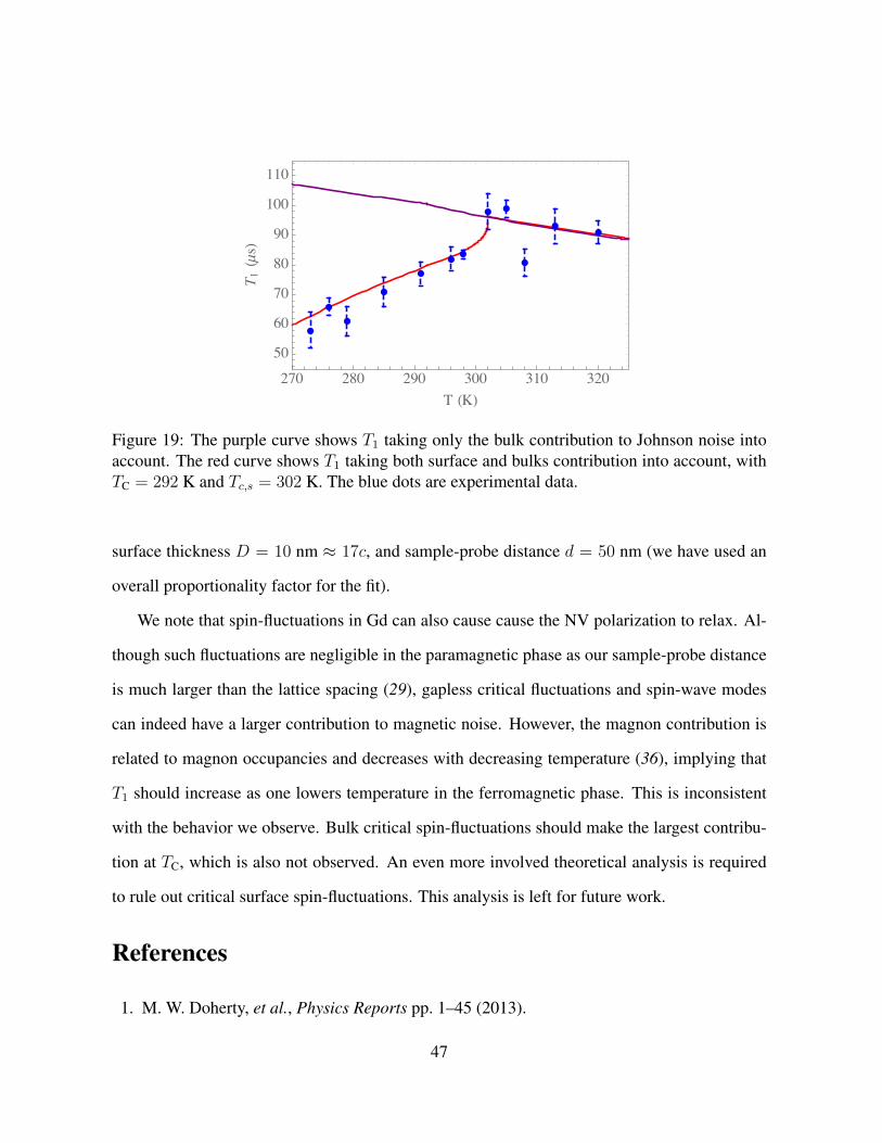
(μ)

Figure 19: The purple curve shows T1 taking only the bulk contribution to Johnson noise intoaccount. The red curve shows T1 taking both surface and bulks contribution into account, withTC = 292 K and Tc,s = 302 K. The blue dots are experimental data.

surface thickness D = 10 nm ≈ 17c, and sample-probe distance d = 50 nm (we have used an

overall proportionality factor for the fit).

We note that spin-fluctuations in Gd can also cause cause the NV polarization to relax. Al-

though such fluctuations are negligible in the paramagnetic phase as our sample-probe distance

is much larger than the lattice spacing (29), gapless critical fluctuations and spin-wave modes

can indeed have a larger contribution to magnetic noise. However, the magnon contribution is

related to magnon occupancies and decreases with decreasing temperature (36), implying that

T1 should increase as one lowers temperature in the ferromagnetic phase. This is inconsistent

with the behavior we observe. Bulk critical spin-fluctuations should make the largest contribu-

tion at TC, which is also not observed. An even more involved theoretical analysis is required

to rule out critical surface spin-fluctuations. This analysis is left for future work.

References

1. M. W. Doherty, et al., Physics Reports pp. 1–45 (2013).

47

2. A. Dreau, et al., Physical Review B 84, 195204 (2011).

3. Y. Feng, D. M. Silevitch, T. F. Rosenbaum, Review of Scientific Instruments 85, 033901

(2014).

4. M. Mito, et al., Phys. Rev. B 67, 024427 (2003).

5. D. Jackson, et al., Review of scientific instruments 74, 2467 (2003).

6. P. L. Alireza, G. G. Lonzarich, Review of Scientific Instruments 80, 023906 (2009).

7. M. Mito, et al., Japanese Journal of Applied Physics 40, 6641 (2001).

8. G. Giriat, W. Wang, J. P. Attfield, A. D. Huxley, K. V. Kamenev, Review of Scientific

Instruments 81, 073905 (2010).

9. K. Takeda, M. Mito, Journal of the Physical Society of Japan 71, 729 (2002).

10. A. Marizy, B. Guigue, F. Occelli, B. Leridon, P. Loubeyre, High Pressure Research 37, 465

(2017).

11. M. P. Pasternak, R. D. Taylor, R. Jeanloz, Journal of Applied Physics 70, 5956 (1991).

12. M. P. Pasternak, et al., Phys. Rev. B 65, 035106 (2001).

13. A. P. Kantor, et al., Phys. Rev. Lett. 93, 215502 (2004).

14. O. Mathon, et al., Journal of Synchrotron Radiation 11, 423 (2004).

15. N. Ishimatsu, et al., Physical Review B 75, 180402 (2007).

16. S. Watanabe, et al., Journal of the Physical Society of Japan 80, 093705 (2011).

17. K. Chen, et al., Phys. Rev. B 97, 235153 (2018).

48

18. E. Rittweger, K. Y. Han, S. E. Irvine, C. Eggeling, S. W. Hell, Nature Photonics 3, 144

(2009).

19. T. Mittiga, et al., Physical Review Letters 121, 246402 (2018).

20. M. S. J. Barson, et al., Nano Letters 17, 1496 (2017).

21. A. Dewaele, P. Loubeyre, M. Mezouar, Physical Review B 70 (2004).

22. L. Oroszlany, A. Deak, E. Simon, S. Khmelevskyi, L. Szunyogh, Physical review letters

115, 096402 (2015).

23. A. Jayaraman, Metals (Elsevier, 1978), vol. 1 of Handbook on the Physics and Chemistry

of Rare Earths, pp. 707 – 747.

24. D. D. Jackson, V. Malba, S. T. Weir, P. A. Baker, Y. K. Vohra, Phys. Rev. B 71, 184416

(2005).

25. D. B. McWhan, A. L. Stevens, Phys. Rev. 139, A682 (1965).

26. T. Iwamoto, M. Mito, M. Hidaka, T. Kawae, K. Takeda, Physica B: Condensed Matter 329-

333, 667 (2003). Proceedings of the 23rd International Conference on Low Temperature

Physics.

27. G. K. Samudrala, G. M. Tsoi, S. T. Weir, Y. K. Vohra, High Pressure Research 34, 385

(2014).

28. J. Akella, G. S. Smith, A. P. Jephcoat, Journal of Physics and Chemistry of Solids 49, 573

(1988).

29. K. Agarwal, et al., Phys. Rev. B 95, 155107 (2017).

49

30. H. E. Nigh, S. Legvold, F. H. Spedding, Phys. Rev. 132, 1092 (1963).

31. P. Jacobsson, B. Sundqvist, Phys. Rev. B 40, 9541 (1989).

32. R. V. Colvin, S. Legvold, F. H. Spedding, Phys. Rev. 120, 741 (1960).

33. V. Y. Bodryakov, A. A. Povzner, O. G. Zelyukova, Physics of the Solid State 41, 1138

(1999).

34. M. E. Fisher, J. S. Langer, Phys. Rev. Lett. 20, 665 (1968).

35. J. B. Kogut, Rev. Mod. Phys. 51, 659 (1979).

36. S. Chatterjee, J. F. Rodriguez-Nieva, E. Demler, ArXiv e-prints p. arXiv:1810.04183

(2018).

50