Imaging with Wireless Sensor Networks

Rob Nowak

Waheed Bajwa, Jarvis Haupt, Akbar Sayeed

Supported by the NSF

What is a Wireless Sensor Network?

• Comm between army units was crucial

• Signal towers built on hilltops

• Wireless comm and coding consisted of smoke signals, fires, flags, cannon fire

e.g., during Ming Dynasty a single column of smoke plus a single gun shot would indicate the approach of a hundred enemy soldiers

Goal: Measure, estimate and convey a physical field

Ex. Temperature, light, pressure, moisture, vibration, sound, gas concentration, position

Wireless Sensor Networks Today (or Tomorrow)

Each node equipped with power source(s)sensor(s) modest computing capabilitiesradio transmitter/receiver

Wireless Sensors

solar cell

battery

radio

GPS module

µµµµprocsensor

What is a Sensor Network?

A network of sensors spatially distributed over- imperial border- forest- Internet- cropland- manufacturing facility- urban environment

For monitoring spatially distributed processes- enemy soldiers- fires- spread of computer viruses- temperature, light, moisture- biological and chemical processes

What is Information Processing in Sensor Networks ?

Extracting, Manipulating, and Communicatingsalient features from raw sensor data and delivering them to a destination

Features:

- location/magnitude of sources- summary statistics - signals, maps & images- decisions

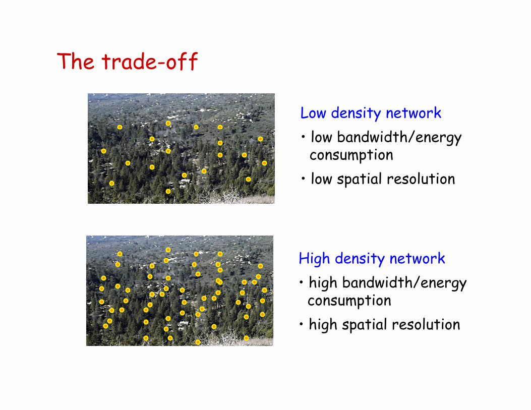
The trade-off

Low density network

• low bandwidth/energyconsumption

• low spatial resolution

High density network

• high bandwidth/energyconsumption

• high spatial resolution

But…

Physical fields are spatially correlated, so information does not grow linearly with network density

Knowledge of correlation (e.g., Slepian-Wolf coding) or in-network processing can significantly reduce number of bits that must be transmitted

The upshot

Basic Trade-off:

Field is more accurately characterized withhigher density sampling, but data rate increases as density increases

u

vR(u,v)Key idea:

As network density increases, correlation between sensor measurements increases,which reduces communication requirements(more communications, but each is shorter)

“data rate” grows linearly with network density, but “information rate” grows is sub-linearly

458 x 300 pixels - coded using only 37 kB

Uncompressed : (458 x 300) x (3 colors x 1 byte) = 412 kB

Compression factor 11:1

Data Compression

A simple field model

i.e., the field is “smooth”

• moisture or pesticide over cropland

• chemical distributionin lake or sea

• biochemical agentin urban environment

Assume that field is k-times continuously differentiable

Pseudocolor depiction of smooth spatial process

Wireless Sensing

Sensor i makes a noisy measurement Y

i

of field at its location Xi

wireless sensors at random locations

• approximate/model/encode f ?• estimate f in presence of noise ?• transmit/reconstruct f at destination ?

How to

GOAL: Reconstruct f at remote destination

Approximating Smooth Fields

Example:

Smooth functions can be locally approximated very well by simple polynomial functions

Approximating Smooth Fields

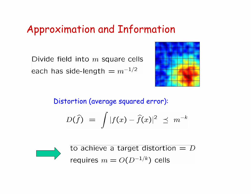
Approximation and Information

Distortion (average squared error):

Rate-Distortion Analysis

log bits

log distortion

Encoding polyfit parameters of each cell requires a fixed number of bits, thus number bits required is proportional to m

k=1

k=2

k=3

“Information” content of field is inversely proportional to smoothness (i.e., increasing k)

Estimating Fields from Noisy Data

1. Divide into m cells

2. Fit polynomial to noisy sensor data in each cell

This accomplishes data compression and denoising

What choice of m is best ?

Noiseless vs. Noisy SensingNoiseless Sensing

Noisy Sensing

What choice of m is best ?

Approximation and Estimation Errors

Partition sensor field into m square cells

Distortion due to partition-based approximation

Distortion due estimating polyfits from noisy data

Estimated polynomial fits fluctuate about optimal Taylor approximations due to noise

Distortion Analysis

Optimal # of cells increases (slowly) with # of sensors

Distortion decreases with # of sensors

Transmitting Information to Destination

Obtaining optimal field reconstruction at destination can be accomplished in several ways:

1. Transmit raw sensor data to destination

2. Compute/transmit local polynomial fits

3. Imaging wireless sensor ensembles; communications and data-fitting combined in single operation

destination

wirelesscomms

Transmission of Raw Data

Transmit raw sensor data to destination using digital comm; destination computes field reconstruction

There are n sensors, so this requires n transmissions;i.e., the number of bits that must be transmitted is O(n)

Communication requirements grow linearly with n

destination

In-Network Processing & Communication

Partition sensor field into cells; local polyfits are computed “in-network” using digital communications

Nodes in each cell self-configure into a wireless network, and cooperatively exchange information to compute polyfit

fixed number of parameters computed per cell

Out-of-Network CommunicationPolyfit parameters are transmitted “out-of-network”

to destination via digital communications

destination

Number of parameters (bits) that must be transmitted to the destination is O(m) = O(n1/(k+1) )

Communication requirements grow sublinearly with n

In-Network Processing & Communication

In-network processing and communications drastically reduce resources (bandwidth, power) required to transmit the field information to a remote destination

Reduction of out-of-network communication resource demands from

O(n) to O(n1/(k+1))

BUT… overhead of forming wireless cooperative networks in each cell consumes a dominant fraction of the system resources

As sensor density increases, we move from a network for sensing to a network for networking !!!

Wireless Sensor Ensembles(Waheed Bajwa, Akbar Sayeed and RN ’05)

destination

• nodes in each cell transmit values via amplitude modulation• no cooperative processing or communications required• transmissions synchronized in each cell to arrive in-phase

An attractive alternative to the conventional sensor network paradigm is a wireless sensor ensemble

processing (averaging) implicitly computed by receive antenna

Ensemble Power Gain

transmitted signalsfrom one cell

received signal

total transmit power ~ n/m A2 receive power ~ (n/m A)2

A = amplitude of each sensor transmission

phase-coherent sum of transmitted signals

Beamforming Gain = n/m = number of sensors in each cell

Ensemble Beamforming

transmitted signalsfrom one cell

received signal

Phase-coherency “beams” energy to receive antenna

phase-coherent sum of transmitted signals

Ensemble Communications and Distortion

approxerror(bias)

sensornoise variance

commnoise variance

Let Ps denote the transmit power per sensor node

we want to choose m and Ps to minimize distortion

Distortion in field reconstruction at destination :

Distortion vs. Power

minimum distortion when

Per Node Power Requirements

power requirements decrease as node density increases!

1. Transmit raw sensor data to destination; destination computes field reconstruction

2. Local polyfits are computed “in-network” and only the estimated parameters are transmitted “out-of-network” to destination

3. Imaging wireless sensor ensembles; communications and data-fitting combined in single operation

Comparison of Three Schemes

… but requires complicatedin-network comms/processing

power requirements grow linearly with network size !

only requires (relatively) simple synchronization of nodes

Power requirements to achieve minimal distortion at destination:

Compressible Signals (Known Subspace)

Smooth fields like this can be well approximated by truncated series expansions (e.g., Fourier, wavelet, etc.)

basis function

coefficient

Truncated series Approximation error

Compressible Signals (Known Subspace)

The same approximation, estimation and communications analysis goes through in this more general case

Nodes synchronize and weight transmissions according to (known) values of corresponding basis functions – desired inner products computed via averaging in receive antenna

transmit powerper coefficient = constant

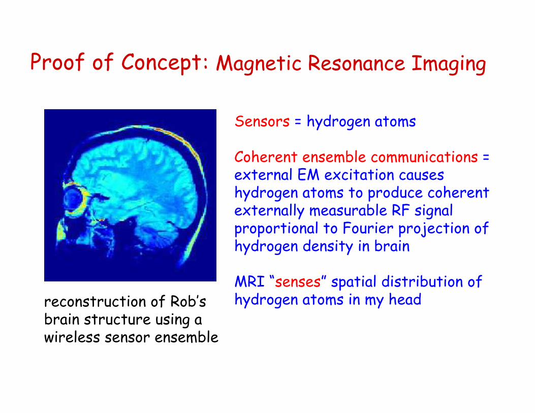
Proof of Concept

reconstruction of Rob’s brain structure using a wireless sensor ensemble

Sensors = hydrogen atoms

Coherent ensemble communications = external EM excitation causes hydrogen atoms to produce coherent externally measurable RF signal proportional to Fourier projection of hydrogen density in brain

MRI “senses” spatial distribution of hydrogen atoms in my head

: Magnetic Resonance Imaging

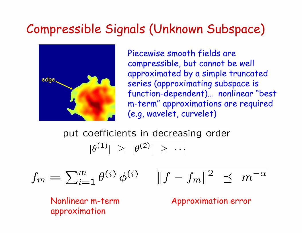
Compressible Signals (Unknown Subspace)

Piecewise smooth fields are compressible, but cannot be well approximated by a simple truncated series (approximating subspace is function-dependent)… nonlinear “best m-term” approximations are required (e.g, wavelet, curvelet)

Nonlinear m-term approximation

Approximation error

edge

Compressive Wireless Sensing(Jarvis Haupt and RN ’05)

destination

destination sends random seed to sensors

each sensor modifies seed according to a local attribute (e.g., location, address)

After r transmissions, destination has r random projections of sensor readings

ANY “compressible” field can be reconstructed from random projections (Candes & Tao ’04, Donoho ’04)

Sensors modulate readings by pseudorandom binary variables and coherently transmit to destination

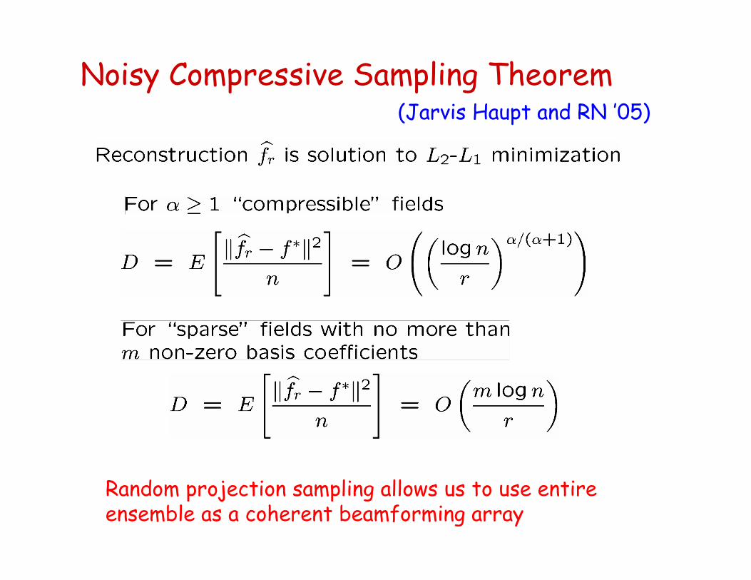
Noisy Compressive Sampling Theorem

Random projection sampling allows us to use entire ensemble as a coherent beamforming array

(Jarvis Haupt and RN ’05)

Distortion vs. Power

Distortion

Total Power

Example: Sparse Signals

known subspace & m optimal projections:

distortion at receiver:

unknown subspace & r > m random projections:

distortion at receiver:

Suppose f is known to be sparse (m non-zero terms in a certain basis expansion)

Random projections are less effective by a factor of r/n ;the fraction of energy they deposit in signal subspace

Example: Lowpass vs. Random Projections

r low frequency Fourier projections:

piecewise smooth field

distortion at receiver:

r random projections:

piecewise smooth fieldwaveletscurvelets

distortion at receiver:

Conclusions

nowak@engr.wisc.edu

www.ece.wisc.edu/~nowak

Complexity (entropy) of field grows far more slowly thanvolume of raw data, as sensor density increases

data rate

informationrate

wireless sensor ensembles offer a promising new architecture for dense wireless sensing

compressive sampling offers advantages ifftarget function is very compressible

Papers

Matched Source-Channel Communication for Field Estimation in Wireless Sensor Networks, W. Bajwa, A. Sayeed and R. Nowak, IPSN 2005, Los Angeles, CA.

Signal Reconstruction from Noisy Random Projections, J. Hauptand R. Nowak, submitted to IEEE Trans. Info. Th., 2005 (short version in Proceedings of 2005 IEEE Statistical Signal Processing Workshop)

www.ece.wisc.edu/~nowak/pubs.html