Imbibition of a liquid droplet on a deformable porous ...math.gmu.edu/~dmanders/WEBDAN/pub_24.pdfImbibition of a liquid droplet on a deformable porous substrate ... Case II diffusion38

PHYSICS OF FLUIDS 17, 087104 �2005�

Imbibition of a liquid droplet on a deformable porous substrateDaniel M. Andersona�

Department of Mathematical Sciences, George Mason University, Fairfax, Virginia 22030

�Received 20 December 2004; accepted 14 June 2005; published online 2 August 2005�

We consider the imbibition of a liquid droplet into a deformable porous substrate. The liquid in thedroplet is imbibed due to capillary suction in an initially dry and undeformed substrate. Deformationof the substrate occurs as the liquid fills the pore space. In our model, a pressure gradient in theliquid across the developing wet substrate region induces a stress gradient in the solid matrix whichin turn leads to an evolving solid fraction and hence deformation. For axisymmetric droplets, weassume that the imbibition and substrate deformation at a given radial position are one-dimensional�in the vertical direction�. The coupling to the droplet geometry leads to axisymmetricconfigurations for the deformed wet substrate. We show that the model chosen to describe thedynamics of the liquid droplet, based in this case on existing models developed for droplet spreadingon rigid porous substrates, has little influence on the resultant swelling or shrinking of thesubstrate—these general trends can be effectively predicted by a one-dimensional imbibition anddeformation model—but does strongly influence the details of the wet substrate shape. Wecharacterize these predictions and in some cases can obtain analytical solutions for the evolution.© 2005 American Institute of Physics. �DOI: 10.1063/1.2000247�

I. INTRODUCTION

In this paper we develop a model for the imbibition of aliquid droplet into a deformable porous substrate. The moti-vation behind this work comes from the inkjet printing in-dustry although the model we develop is general in natureand may be suitable for more simple systems such as a purefluid penetrating into a dry sponge. Our interest here is theinteraction between a fluid droplet and the receiving sub-strate �paper, film, etc.� from the point at which the droplet isin static contact with the substrate. The present study buildson existing models for imbibition of droplets into rigid sub-strates and models for one-dimensional deformation.

Imbibition of fluid into a rigid porous substrate is both aclassical problem and a problem of current technological in-terest. The widely used Lucas–Washburn model1 for liquidimbibition into a porous material is based on the assumptionthat the porous material can be modeled as a collection ofvertically arranged cylindrical capillary tubes. The flowthrough each capillary tube is taken as Poiseuille flow sub-ject to a pressure drop from one end of liquid column to theother. For liquid penetration due to capillary pressure in thetubes, a t1/2 power law characterizes the depth of penetrationinto the porous material.

Recently, Clarke et al.2 described droplet spreading andimbibition using experimental and analytical techniques. Theexperiments were conducted using a picoliter spreading andabsorption instrument that produced droplets with an inkjetprinter head. The liquid droplets under consideration in-cluded water and an aqueous solution of glycerol and hex-elene glycol. The substrates were microporous filter mem-branes with mean pore diameters on the order of 0.1 �m.Spreading was modeled by an equation, previously applied

a�
Electronic mail: [email protected]
1070-6631/2005/17�8�/087104/22/$22.50 17, 08710

Downloaded 30 Aug 2005 to 129.174.45.159. Redistribution subject to

to spreading on smooth impermeable substrates,3 relating thespeed of the contact line to the contact angle. The penetrationwas assumed to be of Lucas–Washburn-type, characterizedby one-dimensional Darcy flow into a rigid substrate wherethe pressure gradient was given by the capillary pressuredivided by the length of the filled pore space. Their observa-tions included situations in which the droplet spreads ini-tially before ultimately receding and being absorbed com-pletely into the substrate. The rate of imbibition was stronglydependent on the wetting characteristics of the fluid and thesubstrate �e.g., the imbibition time for water was four ordersof magnitude longer than the lower surface tension aqueoussolution�.

Holman et al.4 examined the spreading and infiltration ofinkjet-printed aqueous polymeric droplets �54- and 63-�mdiameter� on a rigid porous ceramic surface �typical meanpore size of 0.1 �m�. A spreading model with empiricallydetermined parameters and a Washburn infiltration modelwere used to model the droplet dynamics. In this system thespreading and infiltration occur on the same time scale. Themaximum extension of the droplet was found to depend onthe characteristics of the substrate.

Davis and Hocking6 examined a variety of differentmodels for spreading and imbibition on porous membranesand substrates. These included cases of perfect and imperfectwetting on completely saturated substrates. The flow in thesubstrate was described by Darcy’s law. They considered thepartially saturated case in which the wetted portion of thesubstrate was assumed to extend to the bottom of the sub-strate �which was modeled as an impermeable boundary� andthe boundary between saturated and unsaturated connectedthe top and bottom of the substrate. Davis and Hocking7

adopt their previous results6 to model the spreading above aninitially dry porous substrate. As in the Lucas–Washburn de-
scription, the substrate was assumed to be made up of verti-
© 2005 American Institute of Physics4-1

AIP license or copyright, see http://pof.aip.org/pof/copyright.jsp

http://dx.doi.org/10.1063/1.2000247

http://dx.doi.org/10.1063/1.2000247

087104-2 Daniel M. Anderson Phys. Fluids 17, 087104 �2005�

cally oriented capillaries, in which no “cross linking” of thecapillaries in the substrate occurred. With this one-dimensional �1D� penetration model they calculated penetra-tion shapes as a function of time. The contact-line speed ofthe droplet on the substrate surface was found to be non-monotonic with respect to the contact angle; they concludedthat no analogous “Tanner-law”-type result applies to spread-ing over dry permeable substrates. In contrast, Clarke et al.2

have used such a condition and obtain agreement with theirexperiments. Consequently, as discussed below in more de-tail, we shall investigate the predictions of both the Davisand Hocking model as well as the Clarke et al. model in thecontext of a deformable substrate.

Starov et al.8 investigated the spreading of liquid drop-lets over porous substrates saturated with the same liquid.They modeled the liquid in the porous substrate using Brink-man’s equation. There was no net penetration of the liquiddroplet since the substrate was saturated, however, liquid ex-change between the droplet and porous substrate was re-ported to be important. Experiments were also undertakenusing silicone oils on substrates of average pore size0.25 �m and porosity of approximately 0.75. Both theoryand experiment indicated that a power law governing theradial spreading applied to the droplet evolution.

Droplet spreading on rigid porous surfaces has also re-cently been examined by Seveno et al.,9 who used moleculardynamics simulations to describe the dynamics of a dropletover a single capillary tube. Their numerical simulations forthis problem provided a validation for a model based onLucas–Washburn dynamics. Their generalization to multiplenoninterconnecting pores characterized both the initialspreading and eventual receding/imbibition of the droplet.

An alternative to Darcy-type or Lucas–Washburn capil-lary flow models for porous substrates is a diffusion-typemodel appropriate for polymer matrix substrates. For ex-ample, Oliver, Agbezuge, and Woodcock10 described amodel for drying inkjet drops based on Fickian diffusion forthe ink absorption into the paper. They included simple mod-els for evaporation from the liquid droplet and evaporationafter complete penetration occurred. Swelling of the paperwas not directly considered, however, such effects were par-tially accounted for through the use of experimentally deter-mined diffusion coefficients. They also conducted experi-ments using a water-based ink on substrates including threedifferent office bond papers, and coated and uncoated Mylar�Xerox� transparency films. Measurements were made ofvolume, contact angle, contact line circularity, and contactarea as a function of time. They suggested that local capillarywicking as well as fiber swelling may play important rolesfor the ink drops on the paper substrates considered. Theproblem of liquid imbibition into paper during coating hasalso been examined through the use of pore networkmodels.11

Selim et al.5 examined drying of water-based inks onplain paper and developed a diffusion-based model forevaporation of the liquid and used a Lucas–Washburn modelfor the penetration into the paper. Using their model andexperimental evidence for two different paper types �“acid-
made rosin-sized paper” and “alkaline-made synthetic-sized

paper”� they found generally that the time scale for penetra-tion is much smaller than that for evaporation. Specifically,they reported that for the “rosin-sized paper �the least pen-etrating paper�” the mass loss in a liquid film due to penetra-tion into the porous substrate was about 100 times greaterthan the mass loss into the vapor phase due to evaporation.They comment that the role of evaporation can be increasedfor nonwater-based inks.

The deformation of a porous material has also been along-studied problem that has attracted the attention of re-searchers in fields ranging from geophysics,12 soilscience,13–20 infiltration processes,21–25 paper and printingindustries26,27 and medical science.28–37 These include situa-tions in which imbibition occurs and also situations of fullysaturated media in which capillarity is of secondary or noimportance. Deformation in systems such as glassy poly-mers, which we do not consider here, can be described byCase II diffusion38 wherein the penetration of organic mate-rial into a polymer matrix, at a sharply defined diffusionfront, swells the polymer.

Early descriptions of deformable porous media includethe work of Biot39 on soil settlement, in which fluid flowbased on Darcy’s law is coupled to a linear elasticity modelfor the solid deformation. Solutions for soil consolidation inone dimension as well as two dimensions under permeable40

and impermeable41 rectangular loads were obtained.Chen and Scriven26 modeled a roll applicator process

appropriate for coating flows in the paper and printing indus-try. Their model treated the flow in the deformable receivingporous region, the flow external to the porous region, andadditionally addresses the effects of air compression andtrapped air in the substrate. Flow was driven both by capil-lary and external pressures. Substrate deformation was mod-eled by assuming that the liquid pressure in the pore spaceand the thickness of the compressed substrate were linearlyrelated. Geometrical considerations then related the substratethickness to the local solid fraction.

In the model we develop here for the droplet geometry,we adopt the formulation for liquid penetration and substrate

deformation of Preziosi et al.,22 who studied the infiltrationof a liquid into porous preforms in the industrial process ofinjection molding. We describe our adaption of their modelin more detail below.

The inkjet printing problem involves a number of fluiddynamic effects, most of which we do not address here. Weshall neglect the effects of evaporation of the fluid. We con-sider only a mechanical interaction between the fluid and thesubstrate and neglect chemical properties of either the fluidor substrate. Additionally, we shall assume that the liquiddroplet is initially at rest so that the dynamics of dropletformation, impact and possible merging of droplets can beneglected. Other issues of importance in the inkjet printingproblem include radial capillary penetration42,43 and configu-rations with a relatively thin substrate6,44 in which the pen-etrating liquid reaches the bottom of the substrate. The focusof the present work will be on a configuration in which pen-etration occurs only in the vertical direction in a substratewhose thickness is much greater than the maximum penetra-
tion depth of the fluid. We further assume that the fluid pen-

087104-3 Imbibition of a liquid droplet Phys. Fluids 17, 087104 �2005�

etrates along a well-defined front and completely displacesthe existing air in the pore space, so that the effects of partialsaturation on the permeability of the media are neglected.

With the complex physical processes of inkjet printingtechnology in mind, we shall direct our attention to the rathermodest goal of developing a model for the imbibition of apure liquid droplet into a deformable porous substrate. As weshall see, despite the long list of simplifications given above,there is still a significant level of complexity in this problem.

In Sec. II we describe the basic model geometry andoutline the governing equations applied in the deformablewet substrate. In Sec. III we describe a reduced set of gov-erning equations for one-dimensional imbibition and defor-mation including boundary conditions appropriate for finiteliquid volumes characteristic of the droplet geometry. Herewe also describe similarity solutions and numerical solutionsfor the wet substrate region. In Sec. IV we describe how theliquid droplet evolution couples to the dynamics of the wetsubstrate region. Here we give results for three different liq-uid droplet evolution models coupled to two different modelboundary conditions for a total of six different characteriza-tions of the droplet substrate interaction problem. We iden-tify the key parameters in the imbibition and deformationprocess. In Sec. V we summarize the results and give con-cluding remarks.

II. MODEL DESCRIPTION

We consider an axisymmetric liquid droplet initially atrest on a dry porous substrate. The fluid in the droplet isimbibed by the substrate due to capillary suction in the porespace of the substrate. We consider also only sufficientlysmall droplets so that the effects of gravity can be neglected.There is an additional overpressure in the liquid droplet dueto curvature of the liquid–vapor interface whose contributionto the overall penetration problem is neglected. This assump-tion is valid when the typical pore size in the substrate ismuch smaller than the droplet diameter. Deformation of thesubstrate occurs as a consequence of the fluid penetration.Specifically, deformation of the substrate is assumed to occuras an isotropic elastic response to the pressure exerted on thesolid matrix by the fluid occupying the pore space. Imbibi-tion continues until the liquid droplet volume is depleted.Simultaneous substrate deformation occurs during the imbi-bition process and further deformation may occur after theliquid is completely imbibed.

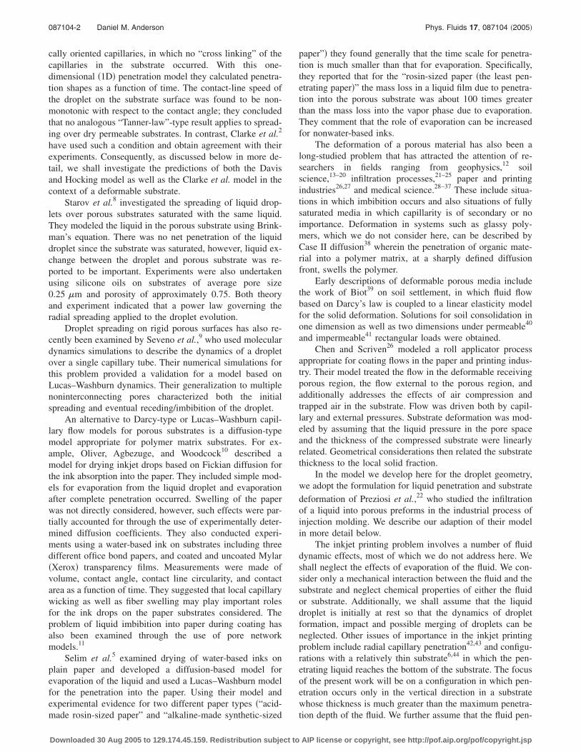
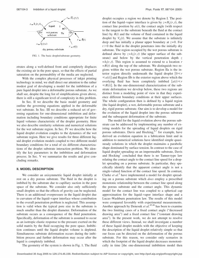
FIG. 1. The basic droplet/substrate geometry.

The geometry of the system is shown in Fig. 1. The fluid


droplet occupies a region we denote by Region I. The posi-tion of the liquid–vapor interface is given by z=HL�r , t�, thecontact line position by a�t�, the contact angle �with respectto the tangent to the substrate beneath the fluid at the contactline� by ��t� and the volume of fluid contained in the liquiddroplet by VL�t�. We assume that the substrate is infinitelydeep and has initially a planar upper boundary at z=0. Fort�0 the fluid in the droplet penetrates into the initially drysubstrate. The region occupied by the wet porous substrate isdefined above by z=hs�r , t� �the upper surface of the sub-strate� and below by the vertical penetration depth z=hl�r , t�. This region is assumed to extend to a location r=R�t� along the top of the substrate. We distinguish two re-gions within the wet porous substrate. Region IIa is the in-terior region directly underneath the liquid droplet �0�r�a�t�� and Region IIb is the exterior region above which theoverlying fluid has been completely imbibed �a�t��r�R�t��. In the one-dimensional characterization of the sub-strate deformation we develop below, these two regions aredistinct from a modeling point of view in that they experi-ence different boundary conditions at their upper surfaces.The whole configuration then is defined by a liquid region�the liquid droplet�, a wet, deformable porous substrate and adry, rigid porous substrate. Our aim is to develop a model forthe evolution of the liquid droplet into the porous substrateand the subsequent deformation of the substrate.

The model for the liquid evolution above the porous sub-strate can be addressed by implementing any number of ex-isting models for the spreading of liquid droplets on rigidporous substrates. Davis and Hocking,6,7 for example, havederived an evolution equation in a lubrication limit and inaddition to numerical solutions have identified simple quasi-steady solutions in which the droplet maintains a parabolicshape dominated by surface tension. In contrast to the case ofliquid droplet spreading on an impermeable substrate, Davisand Hocking7 concluded that there is no Tanner-type lawrelating the contact angle to the contact line speed for a drop-let spreading on a porous substrate. In particular, they spe-cifically identify that the apparent contact angle is not asingle-valued function of the contact line speed. In contrast,Clarke et al.2 have implemented a model for droplet spread-ing on a porous substrate which does employ a prescribedmonotonic relationship between the contact line speed alongthe porous substrate and the contact angle. This dynamicmodel for the contact line was coupled to a spherical capapproximation for the liquid–vapor interface shape and aLucas–Washburn penetration law. The results of this modelwere compared favorably with experimental measurements.Another approach by Denesuk et al.45,46 has been to examinethe two limiting cases of a fixed contact angle �“decreaseddrawing area”� and a fixed contact line �“constant drawingarea”�. In the present work, we do not attempt to resolvethese different views. Instead, we shall investigate a numberof these liquid droplet models with the objective of keepingthe description of the liquid droplet relatively simple so thatour focus can be directed on the deformation of the poroussubstrate. For this reason, we consider only scenarios inwhich the footprint of the liquid droplet decreases monotoni-
cally in time �the one-dimensional imbibition model then


also implies that R�t�=R0 for all time�. This excludes thescenario in which the liquid droplet spreads initially beforereceding. For droplets that recede monotonically in time, weshall find that the deformed substrate underneath the liquiddroplet �i.e., in Region IIa� is always planar. Specific detailson these models are given in Sec. IV.

We now turn our attention to the porous substrate. Weshall assume that when the porous substrate is dry it is rigidand has a constant solid fraction �0. We further assume thatthe fluid penetrates along a well-defined front and com-pletely displaces the existing air in the pore space, so that theeffects of partial saturation on the permeability of the mediacan be neglected. We assume that the air moving through thedry porous substrate meets with no resistance and hence itseffect on the motion of the liquid phase is negligible. Con-sequently, our primary objective will be to formulate govern-ing equations that apply in the wet porous substrate and theassociated interfacial conditions at the penetration front andat the deformed substrate surface. The model we adopt herefollows closely existing substrate deformation models usedby a number of authors,12,21,33,47 which have been developedwith a variety of applications in mind. The present descrip-tion follows most closely the model of Preziosi, Joseph, andBeavers.22 We describe our adaptation of this model to thepresent context below.

The variables of interest in the wet porous medium arethe solid volume fraction �, the velocity of the liquid phaseu� l, the velocity of the solid phase u�s, the liquid pressure pand the stress in the solid �. Mass balance arguments appliedto the solid and liquid phases under the assumption that thedensity of each phase is constant lead to the two continuityequations

��

�t+ � · ��u�s� = 0, �1�

��

�t− � · ��1 − ��u� l� = 0. �2�

The relative velocity u� l−u�s is related to the liquid pressuregradient through Darcy’s law given by

u� l − u�s = −K��

�1 − �� p , �3�

where K�� is the permeability which is taken to be a func-tion of the local solid volume fraction, � is the dynamicviscosity of the fluid, and the factor 1−� �porosity� entersbecause Darcy’s law applies to the volume flux. We specifythe liquid and solid velocity vectors in terms of axisymmetric�r ,z� components as u� l= �ul ,wl� and u�s= �us ,ws�. As de-scribed by Preziosi et al. these equations couple to momen-tum balances for the liquid and solid constituents. A reducedform of these combined momentum equations states that astress equilibrium is maintained in the wet substrate. In par-ticular, there is a balance of the stress in the solid with the
pressure exerted by the surrounding liquid expressed by

0 = − � p + � · � , �4�

where � is the excess stress tensor for the fluid–solid mix-ture and p is the pressure in the liquid phase. Even with thissimplification, which, among other things neglects inertialeffects, there is an important question of how one models thestress �. Preziosi et al. suggested a number of models for �including modeling the solid as a Voight–Kelvin solid or asan anelastic material. We adopt the assumption that the solidcan be treated as an isotropic elastic material where the stresstensor is taken to have the form

� = ��I , �5�

where the � is assumed to be a function of the solid volumefraction alone, ��. Preziosi et al. have justified this for theone-dimensional case. We apply it here in higher dimensions,although in the simplification that follows below, our defor-mation model will be reduced to one-dimensional deforma-tion. Barry and Aldis33 employ an equivalent one-dimensional model for the stress. A similar approach wasalso adopted by Fitt et al.,27 who took the substrate deforma-tion to be one-dimensional and expressed the stress as afunction of the solid fraction. Both Preziosi et al. and Som-mer and Mortensen21 make use of an empirically determined�� relation for their calculations. Spiegelman12 adopts thesame stress equilibrium, but assumes that the stress in thesolid is that of a compressible, highly viscous fluid.

Boundary conditions at the liquid penetration front z=hl�r , t� include

u� l · n̂ =1

�1 + ��hl/�r�2

�hl

�t, �6�

p = pA + pc. �7�

The first condition states that the geometric position of thepenetration front moves with the normal fluid velocity there.The second is a condition on the fluid pressure involving thecapillary pressure pc and atmospheric pressure pA. The cap-illary pressure pc can be thought of as that used by Davis andHocking7 for one-dimensional capillaries −� cos � /b �where� is the surface tension, � is the contact angle in the capillaryand b is the capillary half-width�, or more generally as−Sf� cos � where Sf is the total surface area of solid–liquidinterface per unit volume;23 we treat pc as a given constant inthe present work.

The boundary conditions on the wet substrate–liquid in-terface z=hs�r , t� for 0�r�a�t� are

u�s · n̂ =1

�1 + ��hs/�r�2

�hs

�t, �8�

p = pA + pL�t� , �9�

� = 0, �10�

where pL is the pressure in the liquid droplet at the interfaceand is generally a function of time. The first condition statesthat the deformed boundary of the substrate moves with the
normal solid velocity there. The second condition specifies


the pressure at the top of the wet substrate as that associatedwith the liquid droplet. Here this arises due to surface tensionand the curvature of the liquid-vapor interface, but more gen-erally involves effects due to gravity and/or an externallyapplied pressure. As mentioned earlier, we shall assume thatthe capillary pressure in the pore space is the dominant pres-sure �i.e., �pc�� pL��. The third condition states that the in-terface between the wet substrate–liquid droplet is stressfree.

In the present investigation we examine two possiblemodels for the evolution of the wet substrate–vapor interfacez=hs�r , t� for a�t��r�R�t�. In the first case �Case A�, weassume that the state of the substrate is “frozen” in place at agiven radial position once the liquid droplet recedes past thatposition. In the second case �Case B�, we assume that the wetsubstrate–vapor interface continues to evolve in such a waythat the solid moves with the fluid there to maintain a wetsubstrate–vapor interface; no “puddles” form at the top of thesubstrate nor does the substrate dry out. This translates to theboundary condition u� l=u�s. The interface position hs�r , t� con-tinues to evolve according to Eq. �8�.

In addition to the above equations and boundary condi-tions for the wet substrate region, there is a global massbalance equation for the liquid in the droplet region and inthe wet substrate region. We denote by VS�t� the geometricvolume occupied by the fluid which has penetrated the solid,defined as

VS�t� = 2�0

R�t�

r�hs�r,t� − hl�r,t��dr . �11�

The actual volume of fluid V*�t� occupying the pore spacemust be adjusted by accounting for the total amount of solidoccupying the same volume. That is,

V*�t� = 2�0

R�t� �hl

hs

�1 − ��r,z,t��r dz dr . �12�

In terms of this, we have a global conservation equation V0

=VL�t�+V*�t�, where V0 represents the initial volume of fluidwhich is constant in time �e.g., we do not consider the effectsof mass loss due to evaporation�.

III. ONE-DIMENSIONAL SUBSTRATE DEFORMATIONSOLUTIONS

We focus on a droplet/substrate geometry in which thehorizontal length scale R0 associated with the wet substrate ismuch larger than the vertical length scale H0 in the wet sub-strate. Additionally, we note that the pressure scale in the wetsubstrate is set by the difference in pressure P= pL− pc

measured between the wet substrate–liquid interface �z=hs�r , t�� and the wet substrate–dry substrate interface �z=hl�r , t��. The capillary pressure scales with the total surfacearea of the solid–liquid interface per unit volume23 in theporous substrate while pL scales with the curvature of theliquid drop. Consequently, P�−pc�0 characterizes thesituation in which the pressure difference across the wet sub-
strate is dictated primarily by capillary suction; we take this

to be the case here. This is consistent with the assumptionthat the typical pore size in the substrate is much smallerthan the droplet diameter.

In this setting the Darcy equation �3� implies that largevertical pressure gradients drive a nearly vertical flow. Thehorizontal flow decouples from the solid and liquid massbalance equations �1� and �2� and we have the followingone-dimensional system of equations for the wet substrate:

��

�t+

�

�z��ws� = 0, �13�

��

�t−

�

�z��1 − ��wl� = 0, �14�

wl − ws = −K��

�1 − ��p

�z, �15�

0 = −�p

�z+

��

�z. �16�

These equations are consistent with the one-dimensionalmodels examined by Preziosi et al.22 and by Barry andAldis33,47 who additionally considered radial flows in cylin-drical and spherical geometries.

Before we discuss boundary conditions for this reducedsystem of equations we note that Eqs. �13�–�16� can be re-duced to a single partial differential equation �PDE� for thesolid volume fraction �, as shown by Preziosi et al. This isaccomplished by subtracting Eq. �14� from Eq. �13� so that� /�z��ws+ �1−��wl�=0 and

�ws + �1 − ��wl = c0�r,t� , �17�

where c0 is an arbitrary function to be determined. Using thisresult and Eq. �15� we find that

ws = c0�r,t� +K��

�

�p

�z, �18�

wl = c0�r,t� −�

1 − �

K��

�p

�z. �19�

By the stress equilibrium statement �16� and the constitutiverelation �=�� we note that �p /�z=�� /�z. There-fore, Eq. �13� can be written as

��

�t+ c0�r,t�

��

�z= −

�

�z�K��

�

��

�z �20�

on hl�r , t��z�hs�r , t�. Equation �20� is equivalent to Eq.�44� in Preziosi et al.22

A. Boundary conditions for Region IIa

The boundary conditions applied at the liquid–wet sub-strate interface z=hs�r , t� for 0�r�a�t� are

ws�hs−,t� =

�hs

�t, �21�

p�h−,t� = pA + pL, �22�
s


��hs−,t� = 0. �23�

The boundary conditions applied at the wet substrate–drysubstrate interface z=hl�r , t� are

wl�hl+,t� =

�hl

�t, �24�

p�hl+,t� = pA + pc. �25�

An expression for c0�r , t� can be derived following the argu-ments in Preziosi et al. which we outline below. Evaluatingand equating c0�r , t�=�ws+ �1−��wl on both sides of thewet–dry substrate interface gives

c0�r,t� = ��hl+�ws�hl

+� + �1 − ��hl+��wl�hl

+�

= �1 − �0�wl�hl+� , �26�

where ��hl−�=�0, ws�hl

−�=0 �the dry substrate is rigid� andwe have assumed that wl�hl

−�=wl�hl+�. Another way of view-

ing the latter assumption is that wv�hl−�=wl�hl

+� where wv isthe vertical component of the vapor velocity in the dry sub-strate. From the above result we obtain their Eq. �28�:

ws�hl+� =

��hl+� − �0

��hl+�

wl�hl+� =

��hl+� − �0

��hl+��1 − �0�

c0�r,t� . �27�

Now Eqs. �18� and �27� imply that

c0�r,t� = −�1 − �0�

�0

�K��1 − ��

� ��

�z�hl

+

. �28�

Equation �20� along with boundary conditions �21�–�25�and the expression for c0�r , t� in Eq. �28� represents a closedsystem. To see this, note that Eq. �16� along with the pressureand stress boundary conditions at z=hs�r , t� imply that thepressure throughout Region IIa is given by

p = �� + pA + pL. �29�

Therefore, the pressure boundary condition at z=hl�r , t� canbe written as �(��hl

+ , t�)= pc− pL=−P. Consequently, theproblem can be reduced to solving Eq. �20� subject to theboundary conditions �(��hs

− , t�)=0 and �(��hl+ , t�)=−P.

Note that we can interpret these two equations as Dirichletboundary conditions on � once the form of �� is specified.That is, we can define �l and �s implicitly through the con-ditions

��s� � 0, ��l� � − P . �30�

The interface positions are found using Eqs. �21� and �24�which we write as

�hs

�t= c0�r,t� +

K��

� ��

�z�hs

−

, �31�

�hl

�t= c0�r,t� −

�K��1 − ��

� ��

�z�hl

+

. �32�

The second condition listed in �30� implies a relationshipbetween �l and P. One may argue that the value of �l

should be determined by local physics near the penetrating
front and should be independent of quantities such as pL. We

shall interpret this condition as the definition of �l �see Eq.�43� which includes our assumed form for �� and treat �l

as an input parameter whose dependence on the problem weinvestigate. We shall find that the value of �l, and in particu-lar its value relative to the dry substrate solid fraction �0, isan indicator of the state of deformation in the final wet sub-strate configuration.

B. Boundary conditions for Region IIb

As mentioned above we consider two models for thesubstrate in this region.

In Case A, we simply freeze the evolution; that is, thereis no additional evolution or substrate deformation in theregion a�r�R. Here the deformed substrate shape is deter-mined by tracking the coordinates �a�t� ,hs(a�t� , t)� for theupper substrate position and the coordinates �a�t� ,hl(a�t� , t)�for the lower substrate position. This situation gives a char-acterization of the deformation that occurs only during theactual imbibition process. This model may reflect results ofmore sophisticated models that include evaporation or otherdrying effects that may retard the motion of the wetsubstrate–air interface.

In Case B, the substrate deformation and liquid penetra-tion continues in response to solid fraction �or deformation�gradients in the wet substrate. Recall that in Region IIa thepressure inside the wet substrate region is given by Eq. �29�.Along the bottom boundary z=hl in Region IIb we have thesame condition on pressure �p= pA+ pc� as for the boundaryz=hl in Region IIa. We additionally assume that the samesolid fraction �l is maintained in this region as well. As aresult, the pressure throughout the wet substrate, includingboth Region IIa and Region IIb is given by Eq. �29�. Otherconditions that remain unchanged for Region IIb are the ki-nematic conditions �21� and �24� as well as the expressionfor c0 in Eq. �28�. A new boundary condition is applied at theinterface z=hs�r , t� which states that the vertical fluid veloc-ity is equal to the vertical solid velocity, wl=ws. Owing toDarcy’s equation and the stress equilibrium balance, thiscondition can be rewritten as �� /�z=0 at this boundary.Physically, this boundary condition states that the wetsubstrate–air interface neither dries out �drying out meansws�wl� nor forms “puddles” �puddles form if wl�ws�. Notethat in general ws�0 so the wet substrate–air interface con-tinues to evolve in response to solid fraction �or deformation�gradients in the wet substrate. This boundary is not assumedto be stress free ��0 in general� and the pressure at theinterface is known via Eq. �29� once the solid fraction � isobtained by solving Eq. �20� subject to the given boundaryconditions.

C. Similarity formulation for Region IIa

Equation �20� subject to the boundary conditions for Re-gion IIa described above admits a solution in terms of the
similarity variable


� =z

2�Dt, �33�

where D has units of length squared per unit time and will bespecified below. Additionally, the interface positions are pla-nar and can be expressed as

hs�t� = 2 s�Dt, hl�t� = 2 l

�Dt . �34�

A standard transformation of Eq. �20� leads to the ordinarydifferential equation �ODE�:

2�d�

d�+

�1 − �0��0

�K��1 − ��D

d�

d��

l+

d�

d�

=d

d� �K��

�D

d�

d�� . �35�

Note that the coefficient of the second term on the left-handside of this equation is a constant. This equation is subject tothe boundary conditions �(�� s

−�)=0 and �(�� l+�)=−P.

The values of s and l are determined by solving the equa-tions

s =1

2�−�1 − �0�

�0 �K��

�1 − ��D

d�

d��

l+

+ K��D

d�

d��

s−� , �36�

l = −1

2 �K��

�0�1 − ��D

d�

d��

l+. �37�

Equations �35�–�37� can be solved numerically once appro-priate expressions for K�� and �� are specified. Preziosiet al.22 have examined solutions of this equation for empiri-cally determined values of �� and K�� corresponding to apolyurethane sponge in experiments of Sommer andMortensen.21

Our objective for this model is in terms of a qualitativecharacterization of possible behavior rather than a quantita-tive analysis for specific materials. Consequently, in the cal-culations that follow we shall make special choices for thefunctions K�� and �� which are consistent with physi-cally realistic trends but at the same time allow for a nearlyanalytical solution to be obtained. In particular, suppose that

K�� =K0

�, �� = m��r − �� , �38�

where K0�0 and m�0 so that ��=−m�0. This perme-ability function is inversely proportional to the solid fraction�regions of higher solid fraction correspond to lower perme-ability and regions of lower solid fraction corresponds tohigher permeability�. We expect this to be a reasonablemodel when the solid fraction is not very near the extremevalues of 0 or 1. The stress function is zero when the solidfraction is at a “relaxed” value of �r �which we take to be aprescribed constant�. The sign choice for m is consistent withthat used in Preziosi et al. Note that from Eq. �29� we then
have p=m��r−��+ pA+ pL so that pressure gradients oppose

solid fraction gradients; increases in the liquid pressure leadto reductions in the solid fraction. Additionally, we chooseD=K0m /� and note that

�K��D

= − 1. �39�

For a typical pore size l=1 �m and a typical surface tension�=30 mN m−1 �e.g., Clarke et al.� we can estimate the cap-illary pressure �pc�� / l�104 Pa. Then m�� /��pc /��104/0.2 Pa�105 Pa. Also, for the system con-sidered by Preziosi et al. an estimate for K0 can be obtainedby their figure 2; K0=�rK��r��0.1�10−11 m2�10−12 m2.Using ��10−3 Pa s gives D�10−4 m2/s.

Now Eq. �35� reduces to

− 2�� − B�d�

d�=

d2�

d�2 , �40�

where B is a constant defined by

B =�1 − �0�

2�0 1

1 − �

d�

d��

l+. �41�

Equation �40� is subject to the boundary conditions

� = �r, at � = s, �42�

� = �l � �r +P

m, at � = l. �43�

The values of s and l simplify in Eqs. �36� and �37� and aregiven by

l =1

2�0 1

1 − �

d�

d��

l+, �44�

s = �1 − �0� l −1

2 1

�

d�

d��

s−. �45�

The solution to Eq. �40� can be written down in terms oferror functions as follows:

�� =erf� s − B� − erf�� − B�erf� s − B� − erf� l − B�

��l − �r� + �r, �46�

where

B = �1 − �0� l, �47�

s =��l − �r�

��erf� s − B� − erf� l − B��

� � 1

�rexp�− � s − B�2�

−�1 − �0�

�0�1 − �l�exp�− � l − B�2�� , �48�

l = −��l − �r�exp�− � l − B�2�

�0�1 − �l��erf� s − B� − erf� l − B��. �49�

The solution to the problem is given by Eq. �46� once
Eqs. �47�–�49� are solved to obtain B, s, and l. We note


that if �B , l , s� is a solution so is �−B ,− l ,− s�. For theimbibition process we require l�0 so that liquid front pen-etrates down into the substrate. In an effort to understand thesolutions of Eqs. �47�–�49� we examine two limiting cases inwhich analytical solutions may be identified. If �l=�r+�where � is a small positive number and �0−�r=O�1�, then

s � �0 − �r

�0 1

2�r�1 − �r��1/2

�1/2,

�50�

l � −�r

�0 1

2�r�1 − �r��1/2

�1/2,

with B��1−�0� l. If �l=�0=�r+�, then a modifiedasymptotic result applies

s �1

2�r 1

2�r�1 − �r��1/2

�3/2,

�51�

l � − 1

2�r�1 − �r��1/2

�1/2,

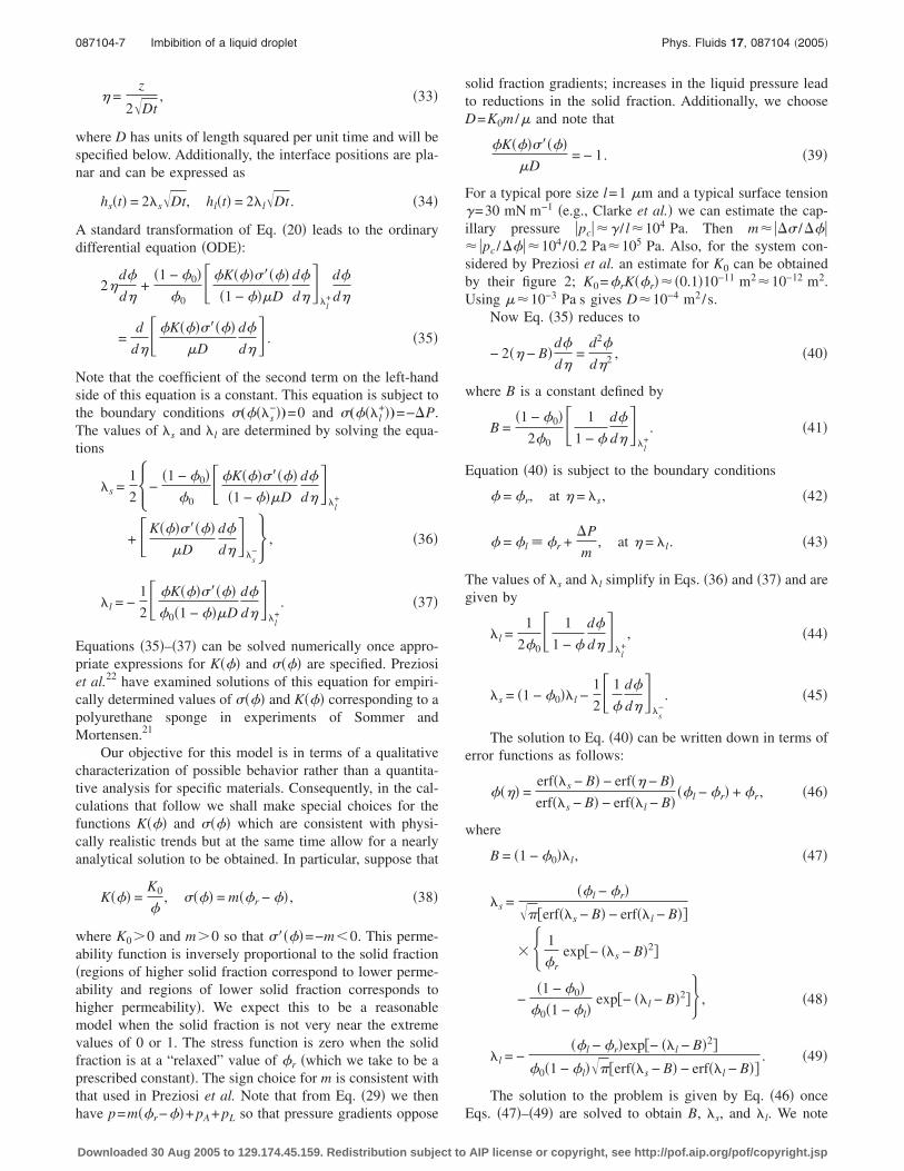
with B��1−�r� l.Figure 2 shows values of s and l plotted as functions

of �l for �0=0.33 and �r=0.1. The solid lines are the nu-merical solutions to Eqs. �47�–�49� while the dashed lineswith open circles indicate the asymptotic results given in Eq.�50�. This figure indicates three important solution regimespossible for one-dimensional imbibition and substrate defor-mation which we shall describe in more detail below whenwe examine the imbibition and deformation of a finite vol-ume of fluid. We can note at this point, however, that it ispossible for s�0 �so that the substrate interface moves
upward—i.e., the substrate swells during imbibition� and

also for s�0 �so that the substrate interface movesdownward—i.e., the substrate shrinks during imbibition�. Athird related scenario emerges when we discuss equilibriumconfigurations of the wet-substrate for finite fluid volumes.

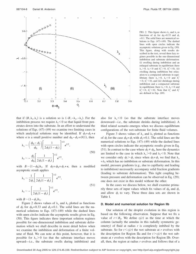
Figure 3 shows values of s and l plotted as functionsof �l for the case �0=�l with �r=0.1. The solid lines are thenumerical solutions to Eqs. �47�–�49� while the dashed lineswith open circles indicate the asymptotic results given in Eq.�51�. In contrast to the case where �l��0, here the dynamicsare limited to the case in which s�0 and l�0. Note thatwe consider only �l��r since when �l=�r we find that s

= l which has no imbibition or substrate deformation. In thismodel, pressure gradients �e.g., due to capillarity and leadingto imbibition� necessarily accompany solid fraction gradients�leading to substrate deformation�. This tight coupling be-tween pressure and deformation can be observed in Eq. �29�;one does not exist in this model without the other.

In the cases we discuss below, we shall examine prima-rily three sets of input values which fix values of �0 and �r

and allow �l to vary. These three data sets are shown inTable I.

D. Model and numerical solution for Region IIb

Our solution of the droplet evolution in this region isbased on the following observation. Suppose that we fix avalue of r�R0. We define tI�r� as the time at which thecolumn �actually the annulus in this radially symmetric ge-ometry� of fluid at radius r is completely imbibed by thesubstrate. So for t� tI�r� the wet substrate at r evolves withthe description for Region IIa and for t� tI�r� the wet sub-strate at r evolves with the description for Region IIb. Over-

FIG. 2. This figure shows s and l asfunctions of �l for �0=0.33 and �r

=0.1. The solid lines are numerical so-lutions to Eqs. �47�–�49�. The dashedlines with open circles indicate theasymptotic solutions given in Eq. �50�.This figure, along with results de-scribed in the text, reveal three key re-gimes possible in the one-dimensionalimbibition and substrate deformation:�i� swelling during imbibition and anenlarged substrate in equilibrium �here s�0, l�0 and hs

��0, hl��0�, �ii�

swelling during imbibition but relax-ation to a compacted substrate in equi-librium �here s�0, l�0 and hs

�

�0, hl��0�, and �iii� shrinkage during

imbibition and a compacted substratein equilibrium �here s�0, l�0 andhs

��0, hl��0�. Note that hs

� and hl�

are defined in Eqs. �69�.

all, then, the region at radius r evolves and follows that of a



one-dimensional imbibition and deformation process with afinite volume supply. In the following discussion we outlinea one-dimensional imbibition and deformation process with afinite volume and then describe how it can be adapted for theaxisymmetric droplet geometry.

For t� tI the fluid is available from the supply �i.e., thedroplet�, the governing equations and boundary conditionsare those of Region IIa and so we apply the similarity solu-tion described in the previous section.

After the fluid is completely imbibed, t� tI, we modelthe evolution of the system with the same equation �20� inthe wet porous substrate but with boundary conditions asdescribed for Region IIb. The initial conditions applied to thesecond stage of the problem at t= tI correspond to the endingconditions of the first stage. So here we solve Eq. �20� sub-ject to the boundary condition �=�l at z=hl and �� /�z=0 atz=hs. The kinematic condition at the interface z=hl�t� is ex-pressed as

TABLE I. This table shows computed values of B, s, and l from thesimilarity solution for three different sets of parameter values for �0, �l,and �r.

Set 1 Set 2 Set 3

�0 0.33 0.33 0.33

�l 0.20 0.33 0.50

�r 0.10 0.10 0.10

B −0.2029 −0.4015 −0.6995

s 0.3752 0.3646 0.1860

l −0.3028 −0.5993 −1.0440


dhl

dt= −

1

�0 �K��

�1 − ��

�z�

hl+. �52�

At the upper boundary, we find that dhs /dt=c0 or

dhs

dt= �1 − �0�

dhl

dt. �53�

As before we consider the case where K��=K0 /� and��=m��r−�� which leads to the equation

��

�t+ D

�1 − �0��0

1

�1 − ��

�z�

hl+

��

�z= D

�2�

�z2 , �54�

subject to the boundary conditions

� = �l, at z = hl�t� , �55�

��

�z= 0, at z = hs�t� , �56�

and

dhl

dt=

D

�0 1

�1 − ��

�z�

hl+, �57�

dhs

dt= �1 − �0�

dhl

dt, �58�

where D=K0m /�. For initial conditions we use the similaritysolution for �, hl, and hs given by Eqs. �46� and �34� for avalue of time t= tI at which the liquid supply is depleted. Forthe strictly one-dimensional problem of imbibition of a finite

FIG. 3. This figure shows s and l asfunctions of �l for the case �0=�l

with �r=0.1. The solid lines are nu-merical solutions to Eqs. �47�–�49�.The dashed lines with open circles in-dicate the asymptotic solutions givenin Eqs. �51�.

volume of fluid and the corresponding substrate deformation,



an analytical expression related to the initial volume of fluidcan be found for tI �see Appendix A�. For the droplet prob-lem this time is a function of radial position tI= tI�r� and isdependent on the particular model used to describe the liquiddroplet evolution. Below we describe a solution to the finiteliquid volume problem and how it can be used for the dropletproblem.

1. Dimensionless system and solution

The system defined by Eqs. �54�–�58� plus initial condi-tions requires numerical solution. In the droplet problem wehave initial times that depend on the radial position tI�r� andso we will need the solution for a range of tI values andcorresponding ranges of values for hs�tI� and hl�tI�. We findthat by first nondimensionalizing this system, a single nu-merical solution can be used to deduce the solution for allinitial conditions of interest.

We introduce dimensionless quantities �denoted by over-bars� into the above system �54�–�58�:

z̄ =z − hl

I

h, t̄ =

D�t − tI��h�2 ,

�59�

h̄l =hl − hl

I

h, h̄s =

hs − hlI

h,

where hlI is the initial value of hl�t�, hs

I is the initial value ofhs�t� and h=hs

I −hlI. Note that h is the thickness of the

deformed wet substrate when the supply of fluid above isdepleted �complete imbibition�.

In terms of these dimensionless quantities the governingequations are

��

�t̄+

1 − �0

�0 1

�1 − ��

�z̄�

z̄=h̄l+

��

�z̄=

�2�

�z̄2 , �60�

subject to the boundary conditions

� = �l, at z̄ = h̄l�t̄� , �61�

��

�z̄= 0, at z̄ = h̄s�t̄� , �62�

and

dh̄l

dt̄=

1

�0 1

�1 − ��

�z̄�

z̄=h̄l+, �63�

dh̄s

dt̄= �1 − �0�

dh̄l

dt̄. �64�

The initial conditions for the interface positions are

h̄l�t̄ = 0� = 0, �65�

h̄s�t̄ = 0� = 1. �66�

The initial condition for � can be derived by first noting that�
��z , tI�=��z /2 DtI� from the similarity solution where

z

2�DtI

=hl

I + z̄�hsI − hl

I�

2�DtI

=2 l

�DtI + 2z̄� s − l�2�DtI

2�DtI

= l + z̄� s − l� . �67�

Therefore, the initial condition for � in dimensionless formis

��z̄, t̄ = 0� = �„ l + z̄� s − l�… , �68�

evaluated using the similarity solution �46�.We have solved numerically the free boundary problem

�60�–�64� subject to initial conditions �65�, �66�, and �68�.The numerical procedure uses an implicit finite differencescheme with second-order accurate differences in space andfirst order in time �based on a similar implementation de-scribed in Anderson, McLaughlin and Miller48�. The result-ing nonlinear system of equations was solved using the non-linear solver hybrd.f �which is based on a modification of thePowell hybrid method, and is available in the MINPACK pack-age at NETLIB �www.netlib.org��.

Before showing the numerical results we point out asimple calculation based on mass conservation applied to theliquid and solid phases that will help interpret the results. Ifone takes as the long-time behavior of the system the state ofuniform solid fraction �l throughout the wet substrate regionthen one obtains the following two formulas for the upperand lower wet substrate interface positions:

hs� = 1 −

�l

�0 V0

1 − �l, hl

� = −�l

�0

V0

1 − �l, �69�

where V0 is the initial volume of fluid per unit area �i.e., theinitial height of the liquid column in this one-dimensionalsetting�. We see that while hl

��0 for all physically relevantparameter values, hs

� may be positive �when �l��0�, nega-tive �when �l��0� or zero �when �l=�0�. With these resultswe can make a full interpretation of the three regimes iden-tified in Fig. 2. In regime �i� where �l��0 swelling occursduring imbibition and the equilibrium configuration corre-sponds to an enlarged substrate �here s�0, l�0 and hs

�

�0, hl��0�. In regime �ii� where �l��0 �and less than the

critical value for which s becomes negative�, swelling oc-curs during imbibition but the equilibrium configuration cor-responds to a compacted substrate �here s�0, l�0 andhs

��0, hl��0�. In regime �iii� where �l is greater than the

critical value for which s becomes negative, shrinkage oc-curs during imbibition and the equilibrium configuration cor-responds to a compacted substrate �here s�0, l�0 andhs

��0, hl��0�. Note that an undeformed equilibrium con-

figuration for the wet substrate �where hs�=0� occurs at a

different value of �l than the situation in which the substrateinterface does not move during imbibition �i.e., where s

=0�. Consequently, it is clear that this model does not in-clude imbibition into a rigid substrate as a special case sincethat scenario has a motionless substrate interface and an un-deformed equilibrium configuration all at a fixed value of �.
We observe these long-time situations in the numerical solu-


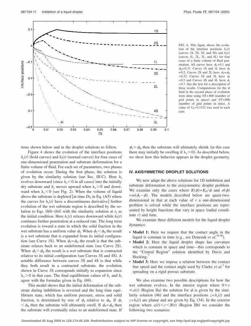
tions shown below and in the droplet solutions to follow.Figure 4 shows the evolution of the interface positions

hs�t� �bold curves� and hl�t� �normal curves� for four cases ofone-dimensional penetration and substrate deformation for afinite volume of fluid. For each set of parameters, two phasesof evolution occur. During the first phase, the solution isgiven by the similarity solution �see Sec. III C�. Here hl

evolves downward �since l�0 in all cases� into the initiallydry substrate and hs moves upward when s�0 and down-ward when s�0 �see Fig. 2�. When the volume of liquidabove the substrate is depleted �at time DtI in Eq. �A5� wherethe curves for hs�t� have a discontinuous derivative� furtherevolution of the wet substrate region is described by the so-lution to Eqs. �60�–�64� with the similarity solution at tI asthe initial condition. Here hs�t� relaxes downward while hl�t�continues further penetration at a reduced rate. The long termevolution is toward a state in which the solid fraction in thewet substrate has a uniform value �l. When �l��0 the resultis a wet substrate that is expanded from its initial configura-tion �see Curve 1S�. When �l=�0 the result is that the sub-strate relaxes back to an undeformed state �see Curve 2S�.When �l��0 the result is a wet substrate that is contractedrelative to its initial configuration �see Curves 3S and 4S�. Anotable difference between curves 3S and 4S is that whilethey both result in a contracted substrate, the evolutionshown in Curve 3S corresponds initially to expansion since s�0 in that case. The final equilibrium values of hs and hl

agree with the formulas given in Eq. �69�.This model shows that the initial deformation of the sub-

strate during imbibition is reversed and the long time equi-librium state, which has uniform pressure, stress and solidfraction, is determined by size of �l relative to �0. If �l

��0 then the substrate will ultimately swell. If �l=�0 then
the substrate will eventually relax to an undeformed state. If

�l��0 then the substrate will ultimately shrink �in this casethere may initially be swelling if s�0�. As described below,we show how this behavior appears in the droplet geometry.

IV. AXISYMMETRIC DROPLET SOLUTIONS

We now adapt the above solutions for 1D imbibition andsubstrate deformation to the axisymmetric droplet problem.We examine only the cases where K��=K0 /� and ��=m��r−��. The models described below are quasi-two-dimensional in that at each value of r a one-dimensionalproblem is solved while the interface positions are repre-sented by height functions that vary in space �radial coordi-nate r� and time.

We examine three different models for the liquid dropletdynamics:

• Model 1: Here we require that the contact angle in theliquid is constant in time �e.g., see Denesuk et al.45,46�.

• Model 2: Here the liquid droplet shape has curvaturewhich is constant in space and time—this corresponds tothe “Central Region” solution identified by Davis andHocking.7

• Model 3: Here we impose a relation between the contactline speed and the contact angle used by Clarke et al.2 forspreading on a rigid porous substrate.

We also examine two possible descriptions for how thewet substrate evolves. In the interior region where 0�r�a�t� �Region IIa� the solution for � is given by the simi-larity solution �46� and the interface positions z=hs�t� andz=hl�t� are planar and are given by Eq. �34�. In the exteriorregion where a�t��r�R�t� �Region IIb� we consider the

FIG. 4. This figure shows the evolu-tion of the interface positions hs�t��curves 1S, 2S, 3S, and 4S� and hl�t��curves 1L, 2L, 3L, and 4L� for fourcases of a finite volume of fluid pen-etration. All curves have �r=0.1 and�0=0.33. Curves 1S and 1L have �l

=0.2, Curves 2S and 2L have �l=�0

=0.33, Curves 3S and 3L have �l

=0.5 and Curves 4S and 4L have �l

=0.7. See the text for a description ofthese results. Computations for the �field in the second phase of evolutionwere done using NX=400 �number ofgrid points in space� and NT=800�number of grid points in time�. Avalue of V0=0.1532 was used in eachcase.

following two scenarios:



• Case A: Here we suppose that wet substrate region ina�t��r�R�t� not directly under the liquid droplet is “fro-zen in.” In this case, the final shape of the wet substrateregion is determined by the locus of points defined by thepenetration depth hl�t� and the liquid contact line a�t� forthe penetration boundary profile and by the deformedheight hs�t� and a�t� for the upper substrate boundary pro-file.

• Case B: The wet-substrate in the exterior region here con-tinues to evolve according to the description and numericalsolution above in Sec. III D 1.

Accordingly, we obtain results for six models �Models1A, 1B, 2A, 2B, 3A, 3B�.

In all of these cases, the substrate deformation problemis coupled to the dynamics of the liquid droplet. Specifically,the liquid region �Region I� and the wet substrate region�Regions IIa and IIb� are coupled through a mass conserva-tion condition applied at the droplet–substrate interface

dVL

dt= 2�1 − ��

0

a

�wl − ws�r dr

= a2� −K��

�

��

�z��hs

= a2D� 1

�

��

�z��hs

= a2� D

2�Dt 1

�

d�

d�� s

. �70�

We note that the corresponding results given in Clark et al.2

by their Eqs. �6� and �7� should have V on the left-hand sidesrather than �V /�t �private communication with A. Clarke,2004�. We note that in their work, they introduced a function��r� defined as the time at which the pore at radius r beginsto fill. That is, if the liquid droplet is spreading, then poresinitially not covered by the liquid droplet may become cov-ered at a later time �; mass transfer from the droplet into thesubstrate at this location only begins at t=��r� rather than att=0. In the cases we discuss in the present paper, we con-sider only receding liquid droplets and so our correspondingvalue of ��r�=0. Equation �70� applies in our case for 0�r�a�t� and so the mass transfer begins at t=0 and ends attI�r�, where tI�r� is defined as the time at which the pore atradius r stops filling.

A. Model 1A: Constant contact angle

We assume that the liquid droplet on the substrate al-ways maintains the shape of a spherical cap. This impliesthat the liquid volume VL�t� at any time t is given by

VL�t� =a3

3 sin3 ��2 − 3 cos � + cos3 �� . �71�

We additionally assume that the contact angle � is constant.
This allows us to write

dVL

dt= a2da

dtg�� , �72�

where

g�� =

sin3 ��2 − 3 cos � + cos3 �� . �73�

For ��1, g��3� /4. If we now use Eq. �72� in Eq. �70�we find that

da

dt=

g�� 1

�

d�

d�� s D

2�Dt, �74�

so that using Eq. �45� we obtain

a�t� = a0 +2 l

g��1 − �0 −

s

l�Dt , �75�

where we note that l�0 for penetration into the substrate sothat a�t� decreases monotonically in time. The droplet disap-pearance time is

tD =1

D a0g��

2 l�1 − �0 − s/ l��2

. �76�

We can now combine Eq. �75� with hl�t�=2 l�Dt and hs�t�

=2 s�Dt in Eq. �34�, noting that the final wet substrate pro-

files for Case A are determined by the locus of points definedby the contact line position with hs�t� for the upper surfaceand with hl�t� for the lower surface. We find that the de-formed substrate shape can be expressed by simple, analyti-cal, expressions:

hl�r� = −g��

�1 − �0 − s/ l��a0 − r� , �77�

hs�r� = − s

l

g��1 − �0 − s/ l�

�a0 − r� , �78�

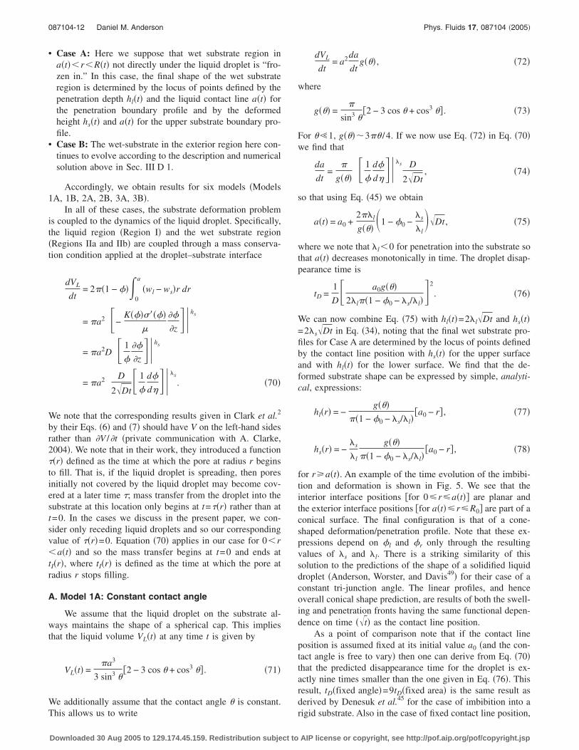
for r�a�t�. An example of the time evolution of the imbibi-tion and deformation is shown in Fig. 5. We see that theinterior interface positions �for 0�r�a�t�� are planar andthe exterior interface positions �for a�t��r�R0� are part of aconical surface. The final configuration is that of a cone-shaped deformation/penetration profile. Note that these ex-pressions depend on �l and �r only through the resultingvalues of s and l. There is a striking similarity of thissolution to the predictions of the shape of a solidified liquiddroplet �Anderson, Worster, and Davis49� for their case of aconstant tri-junction angle. The linear profiles, and henceoverall conical shape prediction, are results of both the swell-ing and penetration fronts having the same functional depen-dence on time ��t� as the contact line position.

As a point of comparison note that if the contact lineposition is assumed fixed at its initial value a0 �and the con-tact angle is free to vary� then one can derive from Eq. �70�that the predicted disappearance time for the droplet is ex-actly nine times smaller than the one given in Eq. �76�. Thisresult, tD�fixed angle�=9tD�fixed area� is the same result asderived by Denesuk et al.45 for the case of imbibition into a
rigid substrate. Also in the case of fixed contact line position,

¯


the final deformed substrate shape is that of a circular diskwhose upper surface is elevated from the original substrateheight. We observe similar shapes as predictions of themodel based on Clarke et al. described in Sec. IV E.

In Case A, the solid fraction profiles at a given radialposition are frozen in once the liquid droplet has recededpast that position. Therefore, in contrast to the results forCase B shown below, the final shapes shown here have non-uniform solid fraction.

B. Model 1B: Constant contact angle

Here we describe the droplet evolution for the casewhere the wet substrate region continues to evolve after theoverlying liquid has been imbibed and the upper surface ofthe wet substrate exposed to air. As described above for Re-gion IIb, the new boundary condition here requires the fluidand solid velocities to be equal to each other at the wetsubstrate–air interface. Below we describe the details of thecalculations.

Our first objective is to identify the time at which aparticular pore at radial position r becomes exposed to air.We set r=a�t� in Eq. �75� and solve the resulting expressionfor t. The result, which we identify as the time tI�r� at whichfluid at radius r has been completely imbibed by the sub-strate, is

DtI�r� = �r − a0�g��2 l�1 − �0 − s/ l�

�2

. �79�

For each radial position we can identify the correspondinginterface heights hs�tI� and hl�tI� �i.e., interface heights at thetime when the liquid at r is completely imbibed by the sub-
strate�. We can determine the evolution of the wet substrate–

air interface and the liquid penetration front at a given radialposition simply by rescaling our one-dimensional solutiondescribed in Sec. III D 1 using the time tI�r� at which thesubstrate interface is first exposed to air and the correspond-ing interface heights hs�tI� and hl�tI�.

In particular, we discretize the radial coordinate on a�t��r�R0. For each of these radial positions we identify tI�r�from Eq. �79� and also identify hs�tI�=2 s�DtI�r� and hl�tI�=2 l�DtI�r�. A dimensionless time t̄=D�t− tI�r�� / �h�tI��2,where h�tI�=2� s− l��DtI�r�, is introduced for each radial

position r and time t and corresponding values of h̄s�t̄� and

hl�t̄� are obtained from a precalculated numerical solution ofEqs. �60�–�66�. Therefore, for any value of t and any value ofr� �a�t� ,R0� we can deduce the appropriate time t̄ at whichthe precalculated solution should be evaluated. Note thatsince the resulting discrete values of t̄ �obtained from dis-crete values of t and r� used here are not exactly those of theprecalculated solution we fit the precalculated numerical so-lution using cubic splines and then evaluate the resultinginterpolation at the required value of t̄. The actual interfacepositions at a given value of r and t that can be plotted are

obtained using hs�r , t�=2 s�DtI�r�+ h̄s�t̄�h�tI� and hl�r , t�=2 l�DtI�r�+ h̄l�t̄�h�tI�.

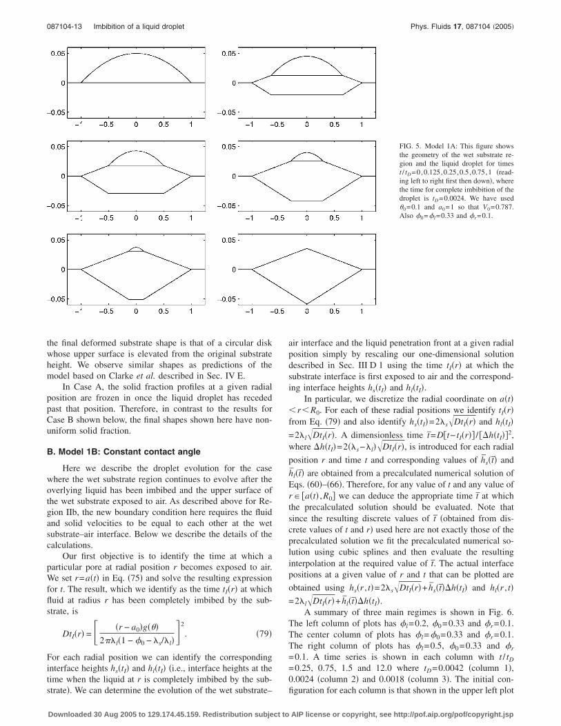
A summary of three main regimes is shown in Fig. 6.The left column of plots has �l=0.2, �0=0.33 and �r=0.1.The center column of plots has �l=�0=0.33 and �r=0.1.The right column of plots has �l=0.5, �0=0.33 and �r

=0.1. A time series is shown in each column with t / tD

=0.25, 0.75, 1.5 and 12.0 where tD=0.0042 �column 1�,0.0024 �column 2� and 0.0018 �column 3�. The initial con-

FIG. 5. Model 1A: This figure showsthe geometry of the wet substrate re-gion and the liquid droplet for timest / tD=0,0.125,0.25,0.5,0.75,1 �read-ing left to right first then down�, wherethe time for complete imbibition of thedroplet is tD=0.0024. We have used�0=0.1 and a0=1 so that V0=0.787.Also �0=�l=0.33 and �r=0.1.

figuration for each column is that shown in the upper left plot



of Fig. 5. In each case there is initial swelling of the substrate�since s�0 here�. However, the long time behavior indi-cates an expanded substrate for �l��0 �left column�, anundeformed substrate for �l=�0 �center column� and a con-tracted substrate for �l��0 �right column�. In all threecases, the final shape has conical features. A fourth case �notshown here� includes the situation in which 0� s� l as inthe fourth curve in Fig. 2 and behaves similarly to the resultsin the right column of plots except that the upper substratesurface moves down, rather than up, initially.

C. Model 2A: Davis and Hocking droplet model

This droplet model follows the one discussed in the“Central region” analysis of Davis and Hocking,7 modifiedfor an axisymmetric geometry. Here the droplet shape has acurvature that is uniform in space and time. In the thin limit,the liquid droplet shape H�r , t� satisfies

�

�r 1

r

�

�rr

�H

�r� = 0. �80�

We note that

H�r,t� =2V0

a04 �a2 − r2� , �81�

satisfies Eq. �80�, boundary conditions H�a , t�=0 and
�H /�r�0, t�=0 and the initial condition

H�r,0� =2V0

a04 �a0

2 − r2� , �82�

where V0 is the initial volume and a0 is the initial contact lineposition. It follows that the corresponding volume of the liq-uid droplet is

VL�t� =V0

a04 a4, �83�

and the apparent contact angle �APP=−�H /�r�a , t� is

�APP =4V0

a04a . �84�

If we now use Eq. �83� in Eq. �70� we find that

d�a2�dt

=a0

4

2V0� 1

�r

d�

d�� s D

2�Dt, �85�

so that integrating and using Eq. �45� gives

a2�t� = a02 +

la04

V01 − �0 −

s

l�Dt . �86�

Again note that l�0 for penetration. This gives the disap-pearance time �when a=0�

tD =1

D V0

la02�1 − �0 − s/ l�

�2

. �87�

Finally, we can combine Eq. �86� with the expressions for

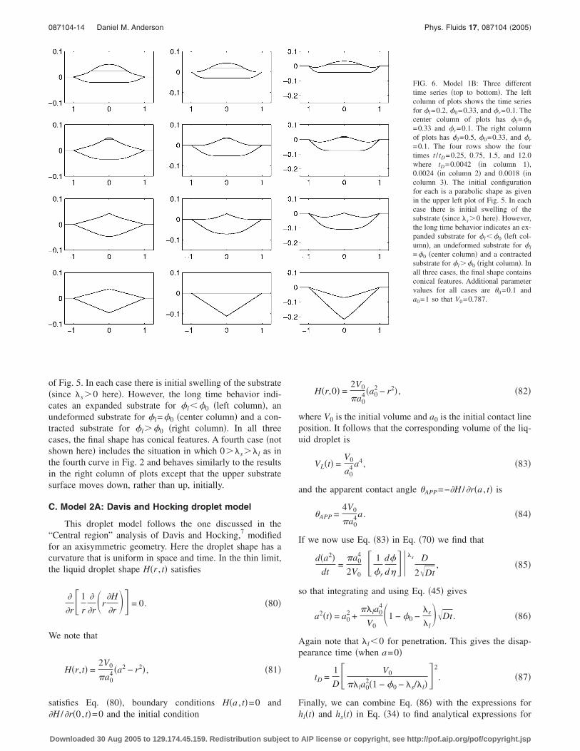
FIG. 6. Model 1B: Three differenttime series �top to bottom�. The leftcolumn of plots shows the time seriesfor �l=0.2, �0=0.33, and �r=0.1. Thecenter column of plots has �l=�0

=0.33 and �r=0.1. The right columnof plots has �l=0.5, �0=0.33, and �r

=0.1. The four rows show the fourtimes t / tD=0.25, 0.75, 1.5, and 12.0where tD=0.0042 �in column 1�,0.0024 �in column 2� and 0.0018 �incolumn 3�. The initial configurationfor each is a parabolic shape as givenin the upper left plot of Fig. 5. In eachcase there is initial swelling of thesubstrate �since s�0 here�. However,the long time behavior indicates an ex-panded substrate for �l��0 �left col-umn�, an undeformed substrate for �l

=�0 �center column� and a contractedsubstrate for �l��0 �right column�. Inall three cases, the final shape containsconical features. Additional parametervalues for all cases are �0=0.1 anda0=1 so that V0=0.787.

hl�t� and hs�t� in Eq. �34� to find analytical expressions for



the spatial profiles of the liquid penetration and the substratesurface deformation:

hl�r� = − 2V0

a04�1 − �0 − s/ l�

��a02 − r2� , �88�

hs�r� = − s

l 2V0

a04�1 − �0 − s/ l�

��a02 − r2� , �89�

for r�a�t�. The dependence of these profiles on �l and �r

enter only through the values of s and l. We again seeplanar fronts for the substrate deformation and liquid pen-etration in the interior, and now parabolic profiles in the ex-terior region as indicated in the example of Fig. 7. As inModel 1A, the solid fraction throughout the wet substrate isnonuniform. As shown in Appendix B, this solution can begeneralized to nonslender geometries. The result is that in-stead of parabolic profiles for the deformation and liquidpenetration fronts, one finds elliptical shapes.

The relationship �APP vs da /dt is qualitatively similar tothat shown in Fig. 3 of Davis and Hocking.7 That is, da /dttends toward infinity as t→0 and as t→ tD; that is, �APP isnot a single-valued function of speed in this model.

D. Model 2B: Davis and Hocking droplet model

Here we describe the droplet evolution predictions forthe case where the wet substrate region continues to evolveafter the overlying liquid has been imbibed and the uppersurface of the wet substrate exposed to air. The approach wetake in obtaining interface profiles is equivalent to the ap-proach described in Sec. IV B and so a description of the
general approach will not be repeated here. We note that a

new formula for tI�r� applies in this case and is given bysetting r=a�t� in Eq. �86�. In this case we have

DtI�r� = �r2 − a02�2 V0

la04�1 − �0 − s/ l�

�2

. �90�

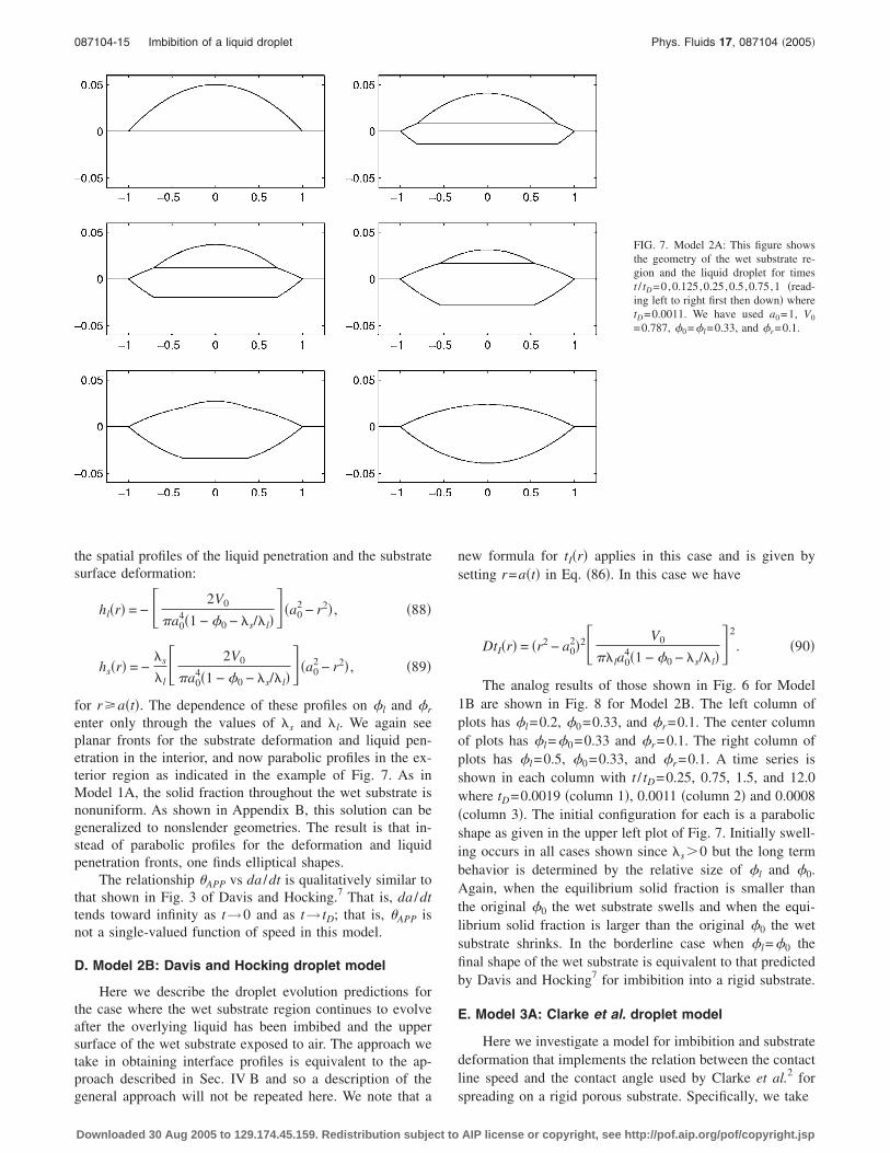
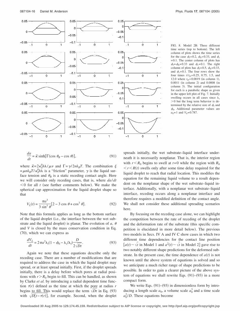
The analog results of those shown in Fig. 6 for Model1B are shown in Fig. 8 for Model 2B. The left column ofplots has �l=0.2, �0=0.33, and �r=0.1. The center columnof plots has �l=�0=0.33 and �r=0.1. The right column ofplots has �l=0.5, �0=0.33, and �r=0.1. A time series isshown in each column with t / tD=0.25, 0.75, 1.5, and 12.0where tD=0.0019 �column 1�, 0.0011 �column 2� and 0.0008�column 3�. The initial configuration for each is a parabolicshape as given in the upper left plot of Fig. 7. Initially swell-ing occurs in all cases shown since s�0 but the long termbehavior is determined by the relative size of �l and �0.Again, when the equilibrium solid fraction is smaller thanthe original �0 the wet substrate swells and when the equi-librium solid fraction is larger than the original �0 the wetsubstrate shrinks. In the borderline case when �l=�0 thefinal shape of the wet substrate is equivalent to that predictedby Davis and Hocking7 for imbibition into a rigid substrate.

E. Model 3A: Clarke et al. droplet model

Here we investigate a model for imbibition and substratedeformation that implements the relation between the contactline speed and the contact angle used by Clarke et al.2 for

FIG. 7. Model 2A: This figure showsthe geometry of the wet substrate re-gion and the liquid droplet for timest / tD=0,0.125,0.25,0.5,0.75,1 �read-ing left to right first then down� wheretD=0.0011. We have used a0=1, V0

=0.787, �0=�l=0.33, and �r=0.1.

spreading on a rigid porous substrate. Specifically, we take



da

dt= �̃ sinh��cos �R − cos �� , �91�

where �̃=2�S0h /�� and �=� /2nkBT. The combination �

=�nkBT /�S0h is a “friction” parameter, � is the liquid sur-

face tension and �R is a static receding contact angle. Herewe will consider only receding cases, that is, where da /dt�0 for all t �see further comments below�. We make thespherical cap approximation for the liquid droplet shape sothat

VL�t� =a3

3 sin3 ��2 − 3 cos � + cos3 �� . �92�

Note that this formula applies as long as the bottom surfaceof the liquid droplet �i.e., the interface between the wet sub-strate and the liquid droplet� is planar. The evolution of a, �and V is closed by the mass conservation condition in Eq.�70�, which we can express as

dVL

dt= 2a2 l�1 − �0 − s/ l�

D

2�Dt. �93�

Again we note that these equations describe only thereceding case. There are a number of modifications that arerequired to address the case in which the liquid droplet mayspread, or at least spread initially. First, if the droplet spreadsinitially, there is a delay before which pores at radial posi-tions with r�R0 begin to fill. This can be handled, as shownby Clarke et al. by introducing a radial dependent time func-tion ��r� defined as the time at which the pore at radius rbegins to fill. This would replace the term �Dt in Eq. �93�

�
with D�t−��r��, for example. Second, when the droplet

spreads initially, the wet substrate–liquid interface under-neath it is necessarily nonplanar. That is, the interior regionwith r�R0 begins to swell at t=0 while the region with R0

�r�R�t� swells only after some time delay required for theliquid droplet to reach that radial location. This modifies theequation for the remaining liquid volume to a result depen-dent on the nonplanar shape of the wet substrate–liquid in-terface. Additionally, with a nonplanar wet substrate–liquidinterface, receding occurs along a nonplanar interface andtherefore requires a modified definition of the contact angle.We shall not consider these additional spreading scenarioshere.

By focusing on the receding case alone, we can highlightthe competition between the rate of receding of the dropletand the deformation rate of the substrate �this specific com-petition is elucidated in more detail below�. The previoustwo models in Secs. IV A and IV C show cases in which twodifferent time dependencies for the contact line position�a�t��t in Model 1 and a2�t��t in Model 2� gave rise totwo notably different shape predictions for the deformed sub-strate. In the present case, the time dependence of a�t� is notknown until the above system of equations is solved and sowe anticipate a much richer range of shape predictions to bepossible. In order to gain a clearer picture of the above sys-tem of equations we shall rewrite Eqs. �91�–�93� in a morecompact form.

We write Eqs. �91�–�93� in dimensionless form by intro-ducing a length scale a0, a volume scale a0

3 and a time scale2

FIG. 8. Model 2B: Three differenttime series �top to bottom�. The leftcolumn of plots shows the time seriesfor the case �l=0.2, �0=0.33, and �r

=0.1. The center column of plots has�l=�0=0.33 and �r=0.1. The rightcolumn of plots has �l=0.5, �0=0.33,and �r=0.1. The four rows show thefour times t / tD=0.25, 0.75, 1.5, and12.0 where tD=0.0019 �in column 1�,0.0011 �in column 2� and 0.0008 �incolumn 3�. The initial configurationfor each is a parabolic shape as givenin the upper left plot of Fig. 7. Initiallyswelling occurs in all cases since s

�0 but the long term behavior is de-termined by the relative size of �l and�0. Additional parameter values area0=1 and V0=0.787.

a0 /D. These equations become



dVL

dt= − � s − �1 − �0� l�

a2

�t0 + t, �94�

da

dt= K sinh��cos �R − cos �� , �95�

d�

dt=

3

a3g�� dVL

dt− a2g��

da

dt� , �96�

where we have differentiated Eq. �92� to obtain the thirdODE for d� /dt. As suggested by Clarke et al. we have in-troduced a small offset time t0 to avoid numerically the sin-gularity at t=0. The new dimensionless parameter appearinghere is K= �̃a0 /D, which describes the competition betweenthe rate of receding and the rate of imbibition. In particular,as K→0 imbibition occurs at a much faster rate than reced-ing while as K→� receding occurs at a much faster rate thanimbibition. Estimates for the parameters �̃ and � were givenby Blake et al.3 They found �̃�102 m/s and �=0.2. Addi-tionally, if we use an initial droplet radius of a0=10−5 m andD�10−4 m2/s then K�10. In order to highlight differentregimes of behavior predicted by this model we shall exam-ine a wide range of values for K. These regimes can besorted into two general classes. As the liquid volume goes tozero and the droplet is completely imbibed, we find that ei-ther a→0 for nonzero � or �→0 for nonzero a.

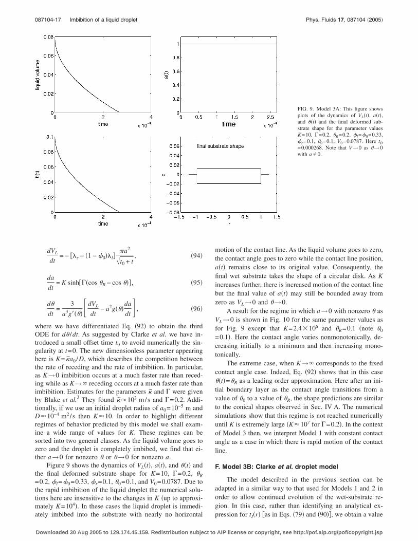
Figure 9 shows the dynamics of VL�t�, a�t�, and ��t� andthe final deformed substrate shape for K=10, �=0.2, �R

=0.2, �l=�0=0.33, �r=0.1, �0=0.1, and V0=0.0787. Due tothe rapid imbibition of the liquid droplet the numerical solu-tions here are insensitive to the changes in K �up to approxi-mately K=104�. In these cases the liquid droplet is immedi-
ately imbibed into the substrate with nearly no horizontal

motion of the contact line. As the liquid volume goes to zero,the contact angle goes to zero while the contact line position,a�t� remains close to its original value. Consequently, thefinal wet substrate takes the shape of a circular disk. As Kincreases further, there is increased motion of the contact linebut the final value of a�t� may still be bounded away fromzero as VL→0 and �→0.

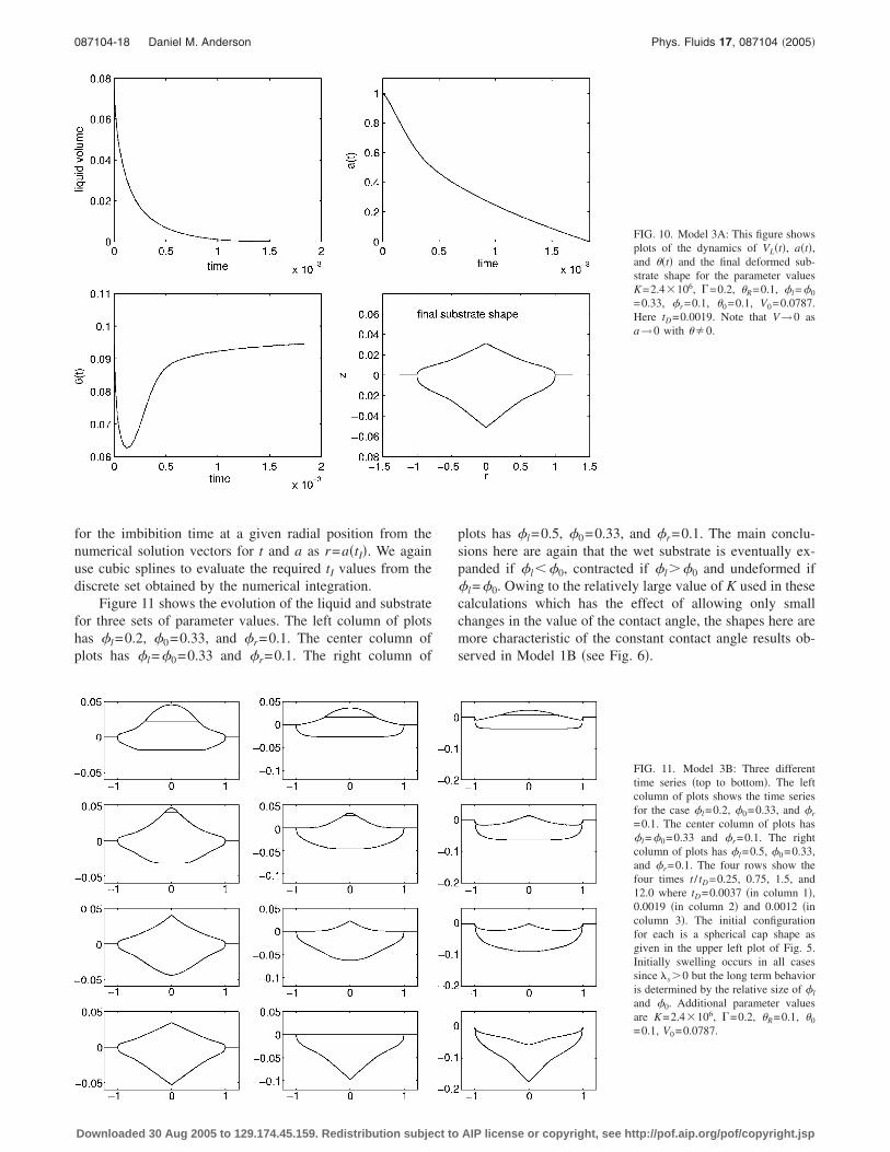
A result for the regime in which a→0 with nonzero � asVL→0 is shown in Fig. 10 for the same parameter values asfor Fig. 9 except that K=2.4�106 and �R=0.1 �note �0

=0.1�. Here the contact angle varies nonmonotonically, de-creasing initially to a minimum and then increasing mono-tonically.

The extreme case, when K→� corresponds to the fixedcontact angle case. Indeed, Eq. �92� shows that in this case��t�=�R as a leading order approximation. Here after an ini-tial boundary layer as the contact angle transitions from avalue of �0 to a value of �R, the shape predictions are similarto the conical shapes observed in Sec. IV A. The numericalsimulations show that this regime is not reached numericallyuntil K is extremely large �K�107 for �=0.2�. In the contextof Model 3 then, we interpret Model 1 with constant contactangle as a case in which there is rapid motion of the contactline.

F. Model 3B: Clarke et al. droplet model

The model described in the previous section can beadapted in a similar way to that used for Models 1 and 2 inorder to allow continued evolution of the wet-substrate re-gion. In this case, rather than identifying an analytical ex-

FIG. 9. Model 3A: This figure showsplots of the dynamics of VL�t�, a�t�,and ��t� and the final deformed sub-strate shape for the parameter valuesK=10, �=0.2, �R=0.2, �l=�0=0.33,�r=0.1, �0=0.1, V0=0.0787. Here tD

=0.000268. Note that V→0 as �→0with a�0.

pression for tI�r� �as in Eqs. �79� and �90��, we obtain a value



for the imbibition time at a given radial position from thenumerical solution vectors for t and a as r=a�tI�. We againuse cubic splines to evaluate the required tI values from thediscrete set obtained by the numerical integration.

Figure 11 shows the evolution of the liquid and substratefor three sets of parameter values. The left column of plotshas �l=0.2, �0=0.33, and �r=0.1. The center column ofplots has �l=�0=0.33 and �r=0.1. The right column of


plots has �l=0.5, �0=0.33, and �r=0.1. The main conclu-sions here are again that the wet substrate is eventually ex-panded if �l��0, contracted if �l��0 and undeformed if�l=�0. Owing to the relatively large value of K used in thesecalculations which has the effect of allowing only smallchanges in the value of the contact angle, the shapes here aremore characteristic of the constant contact angle results ob-served in Model 1B �see Fig. 6�.

FIG. 10. Model 3A: This figure showsplots of the dynamics of VL�t�, a�t�,and ��t� and the final deformed sub-strate shape for the parameter valuesK=2.4�106, �=0.2, �R=0.1, �l=�0

=0.33, �r=0.1, �0=0.1, V0=0.0787.Here tD=0.0019. Note that V→0 asa→0 with ��0.

FIG. 11. Model 3B: Three differenttime series �top to bottom�. The leftcolumn of plots shows the time seriesfor the case �l=0.2, �0=0.33, and �r

=0.1. The center column of plots has�l=�0=0.33 and �r=0.1. The rightcolumn of plots has �l=0.5, �0=0.33,and �r=0.1. The four rows show thefour times t / tD=0.25, 0.75, 1.5, and12.0 where tD=0.0037 �in column 1�,0.0019 �in column 2� and 0.0012 �incolumn 3�. The initial configurationfor each is a spherical cap shape asgiven in the upper left plot of Fig. 5.Initially swelling occurs in all casessince s�0 but the long term behavioris determined by the relative size of �l

and �0. Additional parameter valuesare K=2.4�106, �=0.2, �R=0.1, �0

=0.1, V0=0.0787.



V. CONCLUSIONS

We have shown that relatively simple models for theinteraction between a liquid droplet and a deformable poroussubstrate can be derived and solved. These models couple aone-dimensional description of imbibition into a deformableporous medium to models for the liquid droplet dynamics.

The one-dimensional deformation model used here isbased on the model of Preziosi et al.22 and is similar toseveral other related models.12,21,33,47 In the present work wehave identified a nearly analytical solution to the one-dimensional deformation problem with simple but represen-tative constitutive equations for the permeability and stressfunctions appearing in the deformation model. These func-tions are input to the deformation model and in principlecould be modified and improved for specific systems. Wehave specifically identified a one-dimensional deformationmodel for a finite fluid volume. While the infinite volumecase predicts deformation and penetration fronts that growindefinitely, our model for a finite fluid volume predicts de-formation initially and then relaxation back to a state withuniform solid fraction. During the imbibition process a simi-larity solution governs the dynamics of the flow. For smallsolid fraction values �l the upper surface of the substraterises and the substrate swells while the fluid penetrates intothe substrate. For very large solid fraction values �l the up-per surface of the substrate becomes depressed and the sub-strate shrinks. Interestingly, the transition from swelling toshrinking based on this criterion differs from that based on along-time equilibrium solution in which the solid fraction �aswell as pressure and stress� in the wet substrate is uniform.This leads to the identification of four notable regimes: �i�the substrate swells initially and eventually relaxes to an ex-panded configuration leaving a bump on the substrate sur-face, �ii� the substrate swells initially and eventually relaxesto an undeformed configuration leaving a perfectly flat sub-strate surface, �iii� the substrate expands initially but ulti-mately relaxes to a compacted configuration leaving a pitalong the substrate surface, and �iv� the substrate shrinksinitially and ultimately relaxes to a compacted state with apit along the substrate surface.

We have investigated the coupling of the droplet imbibi-tion and one-dimensional substrate deformation to three dif-ferent models for the droplet evolution. For each of thesethree models we have shown solutions for two different sce-narios involving evolution of the wet substrate–air interface;Case A freezes all further evolution and Case B allows fur-ther evolution based on the assumption that the wetsubstrate–air interface neither dries out nor disappears undera puddle. In Case A, the final state involves a deformed sub-strate characteristic of the similarity solution described forthe one-dimensional imbibition and substrate penetration.Here the solid fraction is “frozen in” at the appearance of thewet substrate–air interface and is nonuniform throughout thewet substrate. In Case B, deformation of the substrate occursduring the imbibition process and a relaxation of this defor-mation back to a state of uniform pressure, stress and solidfraction continues after the droplet has been completely im-
bibed. While the initial growth is governed by the dynamics

of the similarity solution, generally the final equilibrium state�expanded, contracted or undeformed� depends on the valueof �l; if �l��0 the end result is swollen substrate, if �l

=�0 then end result is an undeformed substrate and if �l

��0 then the end result is a shrunken substrate.The primary effect of the specific droplet dynamics

model lies not in whether or not the substrate swells, shrinksor remains undeformed but in the details of the predictedshape. In Model 1 �constant contact angle� the substrateshapes �deformed or undeformed� have conical features. InModel 2 �Hocking and Davis model with constant curvature�the substrate shapes are characterized by parabolic features.In Model 3 �Clarke et al. model� two characteristic regimesare observed. The regime of “fast” receding is characteristicof the constant contact angle case where a→0 as VL→0�and ��0� while the regime of “slow” receding can be re-lated to a fixed contact line case where �→0 as VL→0 �anda�0�. Generally, we find receding retards imbibition. Thiscan be understood by noting that the quantity of fluid takenup by the substrate is proportional to the contact area �andhence the radial position of the contact line squared�. Thesetwo limiting cases noted above for a deformable substrate arethe same as the “decreased drawing area” �fixed contactangle� and the “constant drawing area” �fixed contact line�examined by Denesuk et al.45,46 for a rigid substrate. Thetrend for disappearance time observed by those authors is thesame as that observed for the present case. Models 2A and2B described in Secs. IV C and IV D on the one hand repre-sents a borderline case �where a→0 and �→0 as VL→0�.However, as pointed out by Davis and Hocking7 the corre-sponding relationship between da /dt and � at the contact linein their model is nonmonotonic and therefore we concludemust necessarily be distinct from Model 3.

Clearly there is an opportunity for experimental work onthese systems. We have derived solutions in the most simplecase—one-dimensional imbibition and deformation of an ini-tially static liquid droplet. Additional complications such asmultispecies effects, evaporation and other drying processes,fully two-dimensional deformation effects, and chemical in-teraction between the liquid and solid phases may be re-quired to connect with observations in actual systems. Ourhope is that experimental investigations and more sophisti-cated models may be motivated by the present work.

ACKNOWLEDGMENTS

D.M.A. acknowledges support from the 3M Non-Tenured Faculty Award Program, the Faculty Summer Re-search Support Program at George Mason University, andNSF Award No. DMS-0306996. The author would also liketo thank D. A. Huntley and S. Mohanty at 3M Corporationfor initially suggesting the investigation of this problem andA. A. Wheeler for helpful discussions in the early stages ofthis work.

APPENDIX A: FINITE VOLUME IMBIBITION TIME

Here we calculate an expression for the time for com-
plete imbibition of a finite volume of fluid penetrating into a


deformable substrate. This calculation extends the results inSec. III D.

In particular, if we denote V̄�t� as the volume per unitarea of the supply of fluid above the substrate, then its rate ofchange can be related to the volume flux into the substrate:

dV̄

dt= ��1 − ��wl − ws��z=hs

. �A1�

Using the one-dimensional flow results we find that

dV̄

dt=

D

��

�z�

hs

=D

�

1

2�Dt�d�

d��

�= s

. �A2�

This equation has the solution

V̄�t� = V0 +1

��d�

d��

�= s

�Dt , �A3�

where V0 is the initial �t=0� volume per unit area �height� ofthe overlying fluid. We can simplify this using expression�45� to find that

V̄�t� = V0 + 2��1 − �0� l − s��Dt . �A4�

Using this result we can define the time, tI at which thesupply of liquid has been completely imbibed into the sub-

strate �when V̄�tI�=0�. We find that

DtI = V0

2��1 − �0� l − s�2

. �A5�

APPENDIX B: MODEL 2A—NONSLENDERGEOMETRIES

Note that one can generalize the solution presented inSec. IV C to nonslender geometries if one still imposes thespherical cap approximation on the liquid droplet shape. Inthis case the final deformation and penetration fronts are el-liptical rather than parabolic. This result holds for liquiddroplets with contact angles of less than 90 degrees �so thatas the droplet is imbibed the contact line position decreasesmonotonically to zero�. We describe this solution below.

Suppose that the liquid droplet position is parametrizedby r=RL�z , t�. Then a spherical cap approximation can bewritten as

RL2 + z − a tan� −

2�2

=a2

sin2 ��B1�

�for example, see Anderson, Forest, and Superfine50�. A so-lution that maintains constant curvature in space and timehas

a

sin �=

a0

sin �0, �B2�

where a0 and �0 are the initial contact line position and initialcontact angle. We assume that �0� /2. The liquid volumein this case is given by Eq. �92�. One can derive by differ-
entiating Eq. �92� and using Eq. �B2� that

dV

dt= a3d�

dt. �B3�

Now using this result and Eq. �93� we find that

a2��1 − �0� l − s�D

�Dt= a3d�

dt. �B4�

Upon using Eq. �B2� one obtains

−sin �0

a0��1 − �0� l − s�

D�Dt

=d

dtcos � . �B5�

This equation can be solved to obtain

cos � = cos �0 −sin �0

a0��1 − �0� l − s�2�Dt . �B6�

Now using a2=a02�1−cos2 �� / sin2 �0, hl=2 l

�Dt and hs

=2 s�Dt we write down expressions for the penetration and

substrate deformation profiles �equating a with radial posi-tion r�

r2 + a0 cos �0

sin �0−

��1 − �0� l − s� s

hs�r��2

=a0

2

sin2 �0,

�B7�

r2 + a0 cos �0

sin �0−

��1 − �0� l − s� l

hl�r��2

=a0

2

sin2 �0.

�B8�

These are elliptical profiles.

APPENDIX C: CASE A—AVERAGE SOLID FRACTION

We note that in the droplet penetration/deformationmodel in Case A the solid fraction and interface positions arefrozen for r�a�t�. This fixes a solid fraction distribution inthe wet substrate which is not uniform and in the model ofCase B continues to drive a flow and cause motion of theboundaries. Here we investigate some properties of the “fro-zen in” solid fraction distribution of Case A. We can deter-mine ��r ,z� using the solution �� with suitable interpre-tation of �=z /2�Dt. If we interpret �=��z , t� with t=a−1�r� �a−1 being the inverse function of a�t��, where

t = a−1�r�

=�r − a0�2

D g��

2 l�1 − �0 − s/ l��2

, for Model 1A,

�C1�

t = a−1�r�

=�r2 − a0

2�2

D V0

la04�1 − �0 − s/ l�

�2

, for Model 2A,

�C2�

then the final distribution of � in the wet substrate is givenby ��r ,z�=��z ,a−1�r�� where hl�r��z�hs�r� and 0�r�a0. We have confirmed by direct integration of Eq. �12�

�
that V �tD�=V0. In this calculation we note that


2�0

a0 �hl�r�

hs�r�

r��r,z�dz dr

= 2 � l

s

��d�� 0

a0

2�Dt dr�= 2�− l�0� −

V0

2 l�1 − �0 − s/ l��

=�0V0

�1 − �0 − s/ l�, �C3�

where t=a−1�r� is given by Eqs. �C1� and �C2�.As we have seen in Secs. IV A and IV C analytical pre-

dictions of the interface positions given by Eqs. �77� and �88�have been obtained. Given these final shapes of the wet anddeformed substrate we can calculate the volume occupied bythe wet substrate region VS�tD� �this includes both solid andliquid�. For both of these models we find that

VS�tD� =1 − s/ l

1 − �0 − s/ lV0, �C4�

where V0 is the initial liquid volume. This formula allows usto identify an average solid fraction in the wet substrate bynoting that the factor multiplying V0 can be interpreted as1/ �1−�ave� where

�ave =�0

1 − s/ l. �C5�

This can also be confirmed by directly averaging ��r ,z� overthe final volume VS �using Eqs. �C3� and �C4��. Using the s=0.3646, l=−0.5993, �r=0.1, and �l=�0=0.33 we findthat �ave�0.21 which falls between the values �r=0.1 and�l=0.33.

1E. W. Washburn, “The dynamics of capillary flow,” Phys. Rev. 17, 273�1921�.

2A. Clarke, T. D. Blake, K. Carruthers, and A. Woodward, “Spreading andimbibition of liquid droplets on porous surfaces,” Langmuir 18, 2980�2002�.

3T. D. Blake, A. Clarke, J. De Coninck, and M. J. de Ruijter, “Contactangle relaxation during droplet spreading: Comparison between molecularkinetic theory and molecular dynamics,” Langmuir 13, 2164 �1997�.

4R. K. Holman, M. J. Cima, S. A. Uhland, and E. Sachs, “Spreading andinfiltration of inkjet-printed polymer solution droplets on a porous sub-strate,” J. Colloid Interface Sci. 249, 432 �2002�.

5M. Sami Selim, V. F. Tesavage, R. Chebbi, and S. H. Sung, “Drying ofwater-based inks on plain paper,” J. Imaging Sci. Technol. 41, 152 �1997�.

6S. H. Davis and L. M. Hocking, “Spreading and imbibition of viscousliquid on a porous base,” Phys. Fluids 11, 48 �1999�.

7S. H. Davis and L. M. Hocking, “Spreading and imbibition of viscousliquid on a porous base. II,” Phys. Fluids 12, 1646 �2000�.

8V. M. Starov, S. R. Kosvintsev, V. D. Sobolev, M. G. Verlarde, and S. A.Zhdanov, “Spreading liquid drops over saturated porous layers,” J. ColloidInterface Sci. 246, 372 �2002�.

9D. Seveno, V. Ledauphin, G. Martic, M. Voué, and J. De Conninck,“Spreading drop dynamics on porous surfaces,” Langmuir 18, 7496�2002�.

10J. F. Oliver, L. Agbezuge, and K. Woodcock, “A diffusion approach formodelling penetration of aqueous liquids into paper,” Colloids Surf., A89, 213 �1994�.

11J. Ghassemzadeh, M. Hashemi, L. Sartor, and M. Sahimi, “Pore networksimulation of imbibition into paper during coating: I. Model develop-
ment,” AIChE J. 47, 519 �2001�.

12M. Spiegelman, “Flow in deformable porous media. Part 1. Simple analy-sis,” J. Fluid Mech. 247, 17 �1993�.

13T. K. Karalis, “Water flow in non-saturated swelling soil,” Int. J. Eng. Sci.31, 751 �1993�.

14S. Achanta, J. H. Cushman, and M. R. Okos, “On multicomponent, mul-tiphase thermomechanics with interfaces,” Int. J. Eng. Sci. 32, 1717�1994�.

15M. A. Murad, L. S. Bennethum, and J. H. Cushman, “A multi-scale theoryof swelling porous media: I. Application to one-dimensional consolida-tion,” Transp. Porous Media 19, 93 �1995�.

16L. S. Bennethum and T. Giorgi, “Generalized Forchheimer equation fortwo-phase flow based on hybrid mixture theory,” Transp. Porous Media26, 261 �1997�.

17M. Kaczmarek and T. Hueckel, “Chemico-mechanical consolidation ofclays: Analytical solutions for a linearized one-dimensional problem,”Transp. Porous Media 32, 49 �1998�.

18D. W. Smith, “One-dimensional contaminant transport through a deform-ing porous medium: Theory and a solution for a quasi-steady-state prob-lem,” Int. J. Numer. Analyt. Meth. Geomech. 24, 693 �2000�.

19M. Kaczmarek, “Chemically induced deformation of a porous layercoupled with advective-dispersive transport. Analytical solutions,” Int. J.Numer. Analyt. Meth. Geomech. 25, 757 �2001�.

20G. P. Peters and D. W. Smith, “Solute transport through a deformingporous medium,” Int. J. Numer. Analyt. Meth. Geomech. 26, 683 �2002�.

21J. L. Sommer and A. Mortensen, “Forced unidirectional infiltration ofdeformable porous media,” J. Fluid Mech. 311, 193 �1996�.

22L. Preziosi, D. D. Joseph, and G. S. Beavers, “Infiltration of initially dry,deformable porous media,” Int. J. Multiphase Flow 22, 1205 �1996�.

23V. J. Michaud, J. L. Sommer, and A. Mortensen, “Infiltration of fibrousperforms by a pure metal: Part V. Influence of preform compressibility,”Metall. Mater. Trans. A 30, 471 �1999�.

24D. Ambrosi and L. Preziosi, “Modeling injection molding processes withdeformable porous preforms,” SIAM J. Appl. Math. 61, 22 �2000�.

25L. Billi and A. Farina, “Unidirectional infiltration in deformable porousmedia: Mathematical modeling and self-similar solution,” Q. Appl. Math.58, 85 �2000�.

26K. S. A. Chen and L. E. Scriven, “Liquid penetration into a deformableporous substrate,” Tappi J. 73, 151 �1990�.

27A. D. Fitt, P. D. Howell, J. R. King, C. P. Please, and D. W. Schwende-man, “Multiphase flow in a roll press nip,” Eur. J. Appl. Math. 13, 225�2002�.

28M. H. Holmes, “A nonlinear diffusion equation arising in the study of softtissue,” Q. Appl. Math. 41, 209 �1983�.

29M. H. Holmes, “Comparison theorems and similarity solution approxima-tions for a nonlinear diffusion equation arising in the study of soft tissue,”SIAM J. Appl. Math. 44, 545 �1984�.

30M. H. Holmes, “A theoretical analysis for determining the nonlinear hy-draulic permeability of a soft tissue from a permeation experiment,” Bull.Math. Biol. 47, 669 �1985�.

31M. H. Holmes, “Finite deformation of soft tissue: analysis of a mixturemodel in uni-axial compression,” J. Biomech. Eng. 108, 372 �1986�.

32M. H. Holmes and V. C. Mow, “The nonlinear characteristics fo soft gelsand hydrated connective tissue in ultrafiltration,” J. Biomech. 23, 1145�1990�.

33S. I. Barry and G. K. Aldis, “Flow-induced deformation from pressurizedcavities in absorbing porous tissues,” Bull. Math. Biol. 54, 977 �1992�.

34T. G. Myers, G. K. Aldis, and S. Naili, “Ion induced deformation of softtissue,” Bull. Math. Biol. 57, 77 �1995�.

35C. Zoppou, S. I. Barry, and G. N. Mercer, “Dynamics of human milkextraction: A comparative study of breast feeding and breast pumping,”Bull. Math. Biol. 59, 953 �1997�.

36X-Y. Zhang, J. Luck, M. W. Dewhirst, and F. Yuan, “Interstitial hydraulicconductivity in a fibrosarcoma,” Am. J. Physiol. Heart Circ. Physiol. 279,H2726 �2000�.

37S. McGuire and F. Yuan, “Quantitative analysis of intratumoral infusion ofcolor molecules,” Am. J. Physiol. Heart Circ. Physiol. 281, H715 �2001�.

38N. L. Thomas and A. H. Windle, “A theory of case II diffusion,” Polymer23, 529 �1982�.

39M. A. Biot, “General theory of three-dimensional consolidation,” J. Appl.Phys. 12, 155 �1941�.

40M. A. Biot, “Consolidation settlement under a rectangular load distribu-tion,” J. Appl. Phys. 12, 426 �1941�.

41
M. A. Biot and F. M. Clingan, “Consolidation settlement of a soil with an


imperveous top surface,” J. Appl. Phys. 12, 578 �1941�.42A. Marmur, “The radial capillarity,” J. Colloid Interface Sci. 124, 301

�1988�.43A. Borhan and K. K. Rungta, “An experimental study of the radial pen-

etration of liquids in thin porous substrates,” J. Colloid Interface Sci. 158,403 �1993�.

44A. Marmur, “Drop penetration into a thin porous medium,” J. ColloidInterface Sci. 123, 161 �1988�.

45M. Denesuk, G. L. Smith, B. J. J. Zelinski, N. J. Kreidl, and D. R. Uhl-mann, “Capillary penetration of liquid droplets into porous materials,” J.Colloid Interface Sci. 158, 114 �1993�.

46
M. Denesuk, B. J. J. Zelinski, N. J. Kreidl, and D. R. Uhlmann, “Dynam-

ics of incomplete wetting on porous materials,” J. Colloid Interface Sci.168, 142 �1994�.

47S. I. Barry and G. K. Aldis, “Radial flow through deformable porousshells,” J. Aust. Math. Soc. Ser. B, Appl. Math. 34, 333 �1993�.

48D. M. Anderson, R. M. McLaughlin, and C. T. Miller, “The averaging ofgravity currents in porous media,” Phys. Fluids 15, 2810 �2003�.

49D. M. Anderson, M. G. Worster, and S. H. Davis, “The case for a dynamiccontact angle in containerless solidification,” J. Cryst. Growth 163, 329�1996�.

50D. M. Anderson, M. G. Forest, and R. Superfine, “A model for a spreadingand melting droplet on a heated substrate,” SIAM J. Appl. Math. 61, 1502
�2001�.

Documents

Imbibition of a liquid droplet on a deformable porous ...math.gmu.edu/~dmanders/WEBDAN/pub_24.pdfImbibition of a liquid droplet on a deformable porous substrate ... Case II diffusion38