IMECE2013-63854 - Semantic Scholar€¦ · IMECE2013-63854 Numerical ... liquid-piston compressor with inserted metal foam are done in the present study. The volume-averaging technique

1 Copyright © 2013 by ASME

Proceedings of the ASME 2013 International Mechanical Engineering Congress and Exposition IMECE2013

Nov. 15-21, 2013, San Diego, CA, USA

IMECE2013-63854

Numerical Investigation of Metal-Foam Filled Liquid Piston Compressor Using a Two-Energy Equation Formulation Based on Experimentally Validated Models

Chao Zhang Department of Mechanical

Engineering University of Minnesota Minneapolis, MN55414 [email protected]

Jacob H. Wieberdink Department of Mechanical


Farzad A. Shirazi Department of Mechanical

Engineering University of Minnesota Minneapolis, MN55414

[email protected]

Bo Yan Department of Mechanical


Terrence W. Simon Department of Mechanical


Perry Y. Li Department of Mechanical

Engineering University of Minnesota Minneapolis, MN55414

[email protected]

ABSTRACT The present study presents CFD simulations of a

liquid-piston compressor with metal foam inserts. The term

“liquid-piston” implies that the compression of the gas is done

with a rising liquid-gas interface created by pumping liquid into

the lower section of the compression chamber. The liquid-piston

compressor is an essential part of a Compressed Air Energy

Storage (CAES) system. The reason for inserting metal foam in

the compressor is to reduce the temperature rise of the gas

during compression, since a higher temperature rise leads to

more input work being converted into internal energy, which is

wasted during the storage period as the compressed gas cools.

Liquid, gas, and solid coexist in the compression chamber.

The two-energy equation model is used; the energy equations of

the fluid mixture and the solid are coupled through an interfacial

heat transfer term. The fluid mixture, which includes both the

gas phase and the liquid phase, is modeled using the Volume of

Fluid (VOF) method. Commercial CFD software, ANSYS

FLUENT, is used, by applying its default VOF code, with

user-defined functions to incorporate the two-energy equation

formulation for porous media.

The CFD simulation requires modeling of a negative

momentum source term (drag), and an interfacial heat transfer

term. The first one is the pressure drop due to the metal foam,

which is obtained from experimental measurements. To obtain

the interfacial heat transfer term, a compression experiment is

done, which provides instantaneous pressure and volume data.

These data are compared to solutions of a zero-dimensional

compression model based on different heat transfer correlations

from published references. By this comparison, a heat transfer

correlation which is most suitable for the present study is chosen

for use in the CFD simulation.

The CFD simulations investigate two types of metal foam

inserts, two different layouts of the insert (partial vs. full), and

two different liquid piston speeds. The results show the

influence of the metal foam inserts on secondary flows and

temperature distributions.

1. INTRODUCTION Metal foam provides large surface area per unit volume. It

can be used to absorb thermal energy in gas compressors for

applications in Compressed Air Energy Storage (CAES).

Integrating the CAES approach in power producing systems can

overcome the mismatch between power demand and power

generation by compressing air during low-power-demand

periods and expanding the compressed air during

high-power-demand periods. An important aspect for efficient

and effective CAES operation is to achieve near-isothermal

compression. A technology of using inter-stage cooling between

compressors proposed in [1] has demonstrated the importance of

cooling in CAES. A study on liquid-piston compression has

shown that liquid piston has an advantage over a traditional

solid piston in terms of power consumption [2]. Another

advantage of the liquid piston is that it does not compromise the

compression ratio or the use of heat-absorbing media in the


compressor, as liquid can flow through porous medium. A

CAES system design proposed in [3] uses hydraulic circuits and

liquid pistons to compress air, making it possible for exploring

advanced cooling methods, such as inserting solid material in

the liquid-piston compressor and using droplet-sprays. Analyses

based on CFD simulations in [4] have shown that compression

efficiency is higher when the compression process is more

isothermal for the same pressure compression ratio. Physically,

the reason for the need of near-isothermal compression is that

typical compression results in a temperature rise of the

compressed air. This temperature rise occurs because part of the

input work is being converted into an increase in internal energy

of air. This thermal energy, however, is wasted during the

storage period as the compressed air cools. This can be clearly

shown by a P-V diagram (Fig. 1). The total work input is

represented by the integral under the curves. The amount of

recoverable energy is represented by the integral under the

isothermal curve. The total work input of a non-isothermal

process (including the

compression and cooling

processes) is always greater

than that of isothermal

compression, but the amount

of recoverable energy is the

same. Therefore, cooling the

air during compression is

important for lowering input

work and maintaining high

compression efficiency. The

present study investigates

compression processes when

metal foams are used as

heat-absorbing media.

Porous media have been shown to be successful

heat-absorbing materials in engineering applications. A

numerical study on a pulse tube cryocooler has demonstrated an

effective regenerator made of porous media [5]. In another study,

porous media are used in catalytic converters and the

performance is shown [6]. A new technique is presented in [7]

which can be used to fabricate one chunk of metal foam of

variable pore size for heat exchanger applications. Although the

optimum porous media distribution for the liquid-piston

compression chamber is currently unknown, the present study

explores the effects of different metal foam layouts in the

chamber.

CFD simulations on fluid flow and heat transfer in a

liquid-piston compressor with inserted metal foam are done in

the present study. The volume-averaging technique based on [8],

a powerful method for simulating flow through porous media

without the need for resolving the pore-scale activities directly,

is applied. The continuity, momentum, and energy equations are

volume-averaged on the scale of a Representative Elementary

Volume (REV) of the porous medium. Instead of resolving the

flow through the exact shape of the porous medium, these

volume-averaged equations are solved. Due to volume

averaging, a negative momentum source term arises in the

momentum equation. This term has been proposed to be

modeled by a Darcian and a Forchheimer extension term [9].

For formulating the energy transport in the porous media,

two methods are available. One method is the one-energy

equation method, which solves an artificial temperature that

represents an “average” of the solid temperature and fluid

temperature [10]. This requires thermal equilibrium between

fluid and solid phases. The other one is the following

two-energy equation method. The volume-averaged energy

equation for each of the solid and fluid phases is solved. They

are coupled through an interfacial heat transfer term. Different

interfacial heat transfer correlations for flow in porous media

have been proposed [11] – [15]. Each of these correlations will

be assessed in this paper.

Application of the two-energy equation method can be

found in a number of single-phase flow studies, including: fully

developed flow through a metal-foam-filled pipe [16], laminar

flow in a channel passing through porous medium made of small

particles [17], a double-pipe heat exchanger with metal foam

inserts [18], and flow through a ceramic structure used in a solar

energy receiver [19]. The present study will apply this method

for a two-phase flow.

A solid piston compressor with a partial insert of a porous

medium has been solved computationally in [20]. It shows that

the porous insert inhibits the formation of flow vortices. The

study has great value for understanding the flow phenomena in

porous media during compression, yet it solves the one-energy

equation model. Because it solves a solid piston compression

problem, the numerical model cannot be used for the present

study where the piston is a liquid column and both the fluids and

solid temperatures are needed a solution.

The Volume of Fluid (VOF) method proposed by [21] can

be used to numerically simulate immiscible multiphase flows.

The volume fraction scalars are solved to track bulk locations of

different fluid phases; one set of momentum and energy

equations are shared by all fluid phases. In a more recent study,

the VOF method has been applied in a study solving, at the pore

scale, two-phase flow in a porous medium [22]. In the present

study, the VOF model and the two-energy equation model are

applied to solve the global-scale fluid flow and heat transfer

problem in a porous medium.

2. PROBLEM FORMULATION A cylindrical, liquid-piston compression chamber is

occupied by a porous metal foam. The present study investigates

two situations: foam in the entire volume and foam in a portion

of the chamber. A schematic of a partially occupied chamber is

shown in Fig. 2. The fully occupied case uses the same

coordinate system and coordinate layout. The compression

chamber is studied in cylindrical coordinates. The 𝑥 axis is

along the centerline of the compression chamber. The

gravitational field points opposite to the axis direction 𝑥. At

time = 0, water pumping into the chamber at location 𝑥 = 0

begins. Boundaries 𝑥 = 𝐿 and 𝑟 = 𝑅 represent walls of the

chamber. For the partial insert case, the metal foam is inserted

over the region of length 𝐿𝑖𝑛𝑠; for the full insert case, the metal

foam is inserted over the entire length 𝐿. The material of the

metal foam is aluminum.

During compression, water, air, and solid coexist in the

chamber. The two-energy equation model for porous media and

the VOF method are used to formulate the transport equations.

Fig.1. Schematic of isothermal

compression vs. non-isothermal

compression


The continuity equation for each of the two fluid phases is

solved. The fluid density of a particular phase that is transported

by the continuity equation is the phase density times its phase

volume fraction, 𝛼. Let subscripts 1 and 2 represent air and

water, respectively. Then, for air:

𝜕𝛼1𝜌1

𝜕𝑡+ ∇ ∙ (𝛼1𝜌1�⃑� ) = 0 (1)

For water, since the density is a constant, the continuity equation

becomes a transport equation of volume fraction only,

𝜕𝛼2

𝜕𝑡+ ∇ ∙ (𝛼2�⃑� ) = 0 (2)

The velocity field and temperature field are shared by air and

water. Thus, one set of momentum and fluid energy equations

are solved, based on the properties of the fluid mixture.

𝜕𝜌�⃑⃑�

𝜕𝑡+ 𝛻 ∙ (𝜌�⃑� �⃑� ) = −𝛻𝑝 + 𝛻 ∙ 𝜏̿ + 𝜌𝑔 + 𝑆 𝑚 (3)

where 𝜌 = 𝛼1𝜌1 + 𝛼2𝜌2 (4)

The stress tensor, 𝜏̿, is based on viscosity of the fluid that is

made up of air and water,

𝜇 = 𝛼1𝜇1 + 𝛼2𝜇2 (5)

The negative momentum source term, 𝑆 𝑚 , represents the

resistance of the metal foam to the flow. It can be modeled based

on a Darcian and a Forchheimer term using the following form

[9]:

𝑆 𝑚 = −𝜇𝜖�⃑⃑�

𝐾−

1

2𝑏𝜌|𝜖�⃑⃑� |𝜖�⃑⃑� (6)

The energy equation for the fluid is,

𝜕𝜖(𝜌𝑐𝑝𝑇)

𝜕𝑡+ 𝜖𝛻 ∙ (�⃑� 𝜌𝑐𝑝𝑇) = 𝜖𝛻 ∙ 𝑘𝑓𝛻𝑇 + ℎ𝑉(𝑇𝑠 − 𝑇) + 𝜖

𝜕𝑝

𝜕𝑡

(7)

where 𝜌𝑐𝑝 = 𝛼1𝜌1𝑐𝑝,1 + 𝛼2𝜌2𝑐𝑝,2 (8)

𝑘𝑓 = 𝛼1𝑘1 + 𝛼2𝑘2 (9)

The volumetric heat transfer coefficient can be written in terms

of surface heat transfer coefficient,

ℎ𝑉 = 𝑎𝑉ℎ𝑠𝑓 (10)

The air density follows the ideal gas law,

𝜌1 =𝑝

ℛ𝑇 (11)

The energy equation for the solid is

(1 − 𝜖)𝜕

𝜕𝑡(𝜌𝑠𝑐𝑠𝑇𝑠) = (1 − 𝜖)𝛻 ∙ 𝑘𝑠𝛻𝑇𝑠 − ℎ𝑉(𝑇𝑠 − 𝑇) (12)

The boundary conditions for velocity and temperature variables

are given in Table 1.

Fig. 2 Schematic of compression chamber with partial insert

Table.1. Boundary conditions for velocity and temperature

�⃑� (𝑥 = 𝐿) = �⃑� (𝑟 = 𝑅) = 0, �⃑� (𝑥 = 0) = ( , 0)

𝑇(𝑥 = 0) = 𝑇(𝑥 = 𝐿) = 𝑇(𝑟 = 𝑅) = 2

𝑇𝑠(𝑥 = 0) = 𝑇𝑠(𝑥 = 𝐿) = 𝑇𝑠(𝑟 = 𝑅) = 2

𝛼1(𝑥 = 0) = 0, 𝛼2(𝑥 = 0) = 1 𝜕𝑇

𝜕𝑟| =

𝜕𝑇𝑠

𝜕𝑟| =

𝜕𝑢

𝜕𝑟| = 0

𝑇𝑠(𝑟 = 𝑅) = 𝑇

For full insert: 𝑇𝑠(𝑥 = 0) = 𝑇(𝑥 = 𝐿) = 𝑇

For partial insert: 𝑇𝑠(𝑥 = 𝐿 − 𝐿1) = 𝑇(𝑥 = 𝐿 − 𝐿1),

𝑇𝑠(𝑥 = 𝐿 − 𝐿1 − 𝐿 ) = 𝑇(𝑥 = 𝐿 − 𝐿1 − 𝐿 )

CFD simulations based on the above formulation require

models for the negative momentum source term, 𝑆 𝑚 , and the

interfacial heat transfer coefficient, ℎ𝑉. In the next section, the

first will be obtained by measuring the pressure drop of the

metal foam, and the second will be selected by comparing

simple, zero-dimensional (Zero-D) model solutions to measured

volume and pressure data from compression experiments. Then,

using the experimentally validated models, eight CFD runs with

different compression speeds, different metal foams (10PPI and

40PPI), and different layouts of the metal foams (full-insert vs.

partial-insert) will be studied.

3. INVESTIGATIONS ON PRESSURE DROP AND HEAT TRANSFER MODELS

3.1. Pressure Drop

The pressure drop values of the metal foams are measured.

A schematic of the experimental setup is shown in Fig. 3 (a). A

fan moves air as shown. Two kinds of metal foams are inserted

and measured for pressure drop: one with 10 pores per inch

(10PPI), and one with 40PPI. They both have 93% porosity. A

picture of the metal foam pieces is shown in Fig. 3 (b). The flow

rate of air can be adjusted by a manual valve. A Sierra TopTrack

822S flow meter is used to measure the volumetric flow rate.

The gauge pressure, also considered as the pressure drop of the

porous foam, is measured from the pressure tap by a

micro-manometer.

Results are shown in Fig. 4. The micro-manometer has an

uncertainty of 0.125Pa. The uncertainty of the measured Darcian

velocity is 1.5%. The data are fit into the form of Eq. (6), from

which the permeability, 𝐾 , and the coefficient in the

Forchheimer term, 𝑏, are obtained:


10PPI metal foam: 𝐾 = 2.3 × 10−7𝑚2, 𝑏 = 5 0.1 𝑚⁄

40PPI metal foam: 𝐾 = . 13 × 10−8𝑚2, 𝑏 = 1152.0 𝑚⁄

(a) Schematic of experimental setup

(b) Metal foam pieces used in the experiment

Fig. 3.Experimental measurement of pressure drop of metal foam

Fig. 4. Pressure drop vs. Darcian velocity from experiments

3.2. Evaluation of Heat Transfer Models

Several porous media heat transfer correlations are

available in the literature. It is not obvious which is most

suitable for this test. For this reason, experiments which

measure the instantaneous pressure and volume during

compression in a liquid-piston chamber with metal foam inserts

were completed. To compare different heat transfer correlations

with the experimental results, selected correlations are

substituted into a Zero-D model to solve for the temperature

trajectories during the compression processes. The trajectories

were compared with the experimental data.

A schematic of the experimental setup is shown in Fig. 5.

Water is circulated in a clockwise direction. A relief valve is

installed between the pump and the rest of the system to limit

pressure to a maximum of 165 psi. An Omega FTB-1412 turbine

flowmeter is used to measure the volume of water that enters the

compression chamber. This flowmeter is capable of measuring

flow rates from 47cm3/s to 470cm

3/s. The control valve is used

to maintain an approximately constant upstream pressure, thus

regulating the flow rate. The control of this valve is done in

MATLAB/Simulink using the built-in Proportional Integrator

(PI) Controller. Due to the nature of the control valve, the flow

rate is only approximately constant. Downstream of the control

valve is the compression chamber. The chamber is

apolycarbonate pipe with a length of 353 mm and an internal

diameter of 50.8 mm. It is marked with graduations so that the

water level in the chamber can be recorded. A PCI-DAS1602/16

16-bit analog input board is used to send and receive signals.

Using xPC target, the I/O board is connected to a

MATLAB/Simulink model for control and data acquisition. The

sampling frequency is chosen to be 4000 Hz to correctly acquire

the signal from the turbine meter. The three measured signals are:

upstream pressure, turbine meter flow rate, and chamber

pressure.

Fig. 5. Experimental setup schematic of liquid-piston compression

Two experimental runs are made, one with the chamber

filled with 10PPI metal foam, and the other with 40PPI metal

foam. The conditions for these runs are given in Table 2. Due to

a difference in the lengths of the compression chamber and the

metal foam inserts, there remains at the bottom of the chamber a

region that does not have insert material. In these experiments,

the liquid piston is brought to the bottom of the metal foam at

the beginning of compression so that the entire active length of

chamber is filled with the metal foam insert. The instantaneous

volume of air in the compression chamber is found by

subtracting the cumulative amount of water added to the

chamber from the initial volume of air. The instantaneous

pressure of the compression chamber air is found directly from

the pressure transducer at the top of the chamber. The

instantaneous temperature is not measured directly; it is

calculated from pressure and volume measurements using the

ideal gas law. Although previous efforts had been made to

measure the air temperature using a thermocouple, the ideal gas

law method is preferred for several reasons. A thermocouple

measurement is only one point in a thermal field that contains

large thermal gradients. Additionally, the relatively fast

temperature change during the transient process is difficult to

capture accurately with the relatively slow responding

thermocouple. Additionally,

The Zero-D numerical model has been used for calculating

the transient bulk temperature and pressure in a compressor with

heat exchanger inserts [23]. The model is used to compare with

experimental results. The model is given by the following

energy equations for air and solid, respectively:


ℎ𝑉𝑉(𝑇𝑎𝑖 − 𝑇𝑠𝑜𝑙𝑖𝑑) = (𝑐𝑣

ℛ+ 1)𝜀𝐴 𝑃 +

𝑐𝑣

ℛ𝜀𝐴 𝑖𝑛𝑉

𝑑𝑃

𝑑𝑉 (13)

𝑐𝑠𝜌𝑠(1 − 𝜀)𝐴 𝑖𝑛𝑑𝑇𝑠𝑜𝑙𝑖𝑑

𝑑𝑉= −ℎ𝑉(𝑇𝑎𝑖 − 𝑇𝑠𝑜𝑙𝑖𝑑) (14)

The two equations are coupled through an interfacial heat

transfer coefficient, ℎ𝑉.

Table 2. Conditions of experimental runs Experimental

Runs

Initial length of

air region (m)

Chamber

radius (m)

Initial and ambient

temperature (K)

10PPI Run 0.294 0.0254 297

40PPI Run 0.272 0.0254 297

Initial

Pressure (Pa)

Compression

time (s)

Average Flow

Rate (m3/s)

10PPI Run 101644 2.54 1. 2 × 10−

40PPI Run 102632 3.78 1.210 × 10−

A number of references have given interfacial heat transfer

correlations often used for porous media. Wakao and Kaguei

proposed a correlation for packed beds of 40% porosity based

on the length scale of particle diameter [11]. The correlation is

converted for use in a form which is based on mean pore

diameter by assuming a ratio of pore volume to particle volume

of 4/6. The converted Wakao and Kaguei correlation reads,

ℎ𝑠𝑓𝑑𝑚

𝑘= 1. 8 + 1.1 (

𝜌𝑢𝐷𝑑𝑚

𝜇) .6𝑃𝑟

1

3 (15)

Kuwahara, et al. proposed a correlation for packed square rods

in cross flow based on the rod edge size [12]. The exact layout

of the porous medium was given. After conversion, the

correlation based on mean pore diameter for a 93% porosity

medium reads,

ℎ𝑠𝑓𝑑𝑚

𝑘= . 8 + 0.2 (


𝜇) .6𝑃𝑟

1

3 (16)

Zukauskas developed heat transfer correlations for cylinders in

cross flow [13]. The correlations have been further modified to

be used for porous media [16]. They are given by:

𝑁𝑢 =ℎ𝑠𝑓𝑑

𝑘𝑓= 0. 6𝑅𝑒𝑑

. 𝑃𝑟 .37, (1 ≤ 𝑅𝑒𝑑 ≤ 0) (17)


𝑘𝑓= 0.52𝑅𝑒𝑑

.5𝑃𝑟 .37, ( 0 ≤ 𝑅𝑒𝑑 ≤ 103) (18)


𝑘𝑓= 0.26𝑅𝑒𝑑

.6𝑃𝑟 .37, (103 ≤ 𝑅𝑒𝑑 ≤ 2 × 105) (19)

where 𝑑 = (1 − 𝑒−1−𝜖

0.04)𝑑𝑓 (20)

𝑑𝑓 is the filament diameter of the metal foam. Nakayama, et al.

developed a heat transfer correlation for open cell porous media

based upon mean pore diameter [14],

ℎ𝑉𝑑𝑚

2

𝑘= 0.0 (

𝜖

1−𝜖)2

3(𝜌𝑢𝐷𝑑𝑚

𝜇)𝑃𝑟 (21)

In addition, they converted two other correlations for open-cell

porous media to be based upon mean pore diameter:

Kamiuto and Yee

ℎ𝑉𝑑𝑚

2

𝑘= 0. 6(


𝜇𝑃𝑟) .791 (𝜖 = 0. 3) (22)

Fu, et al.

ℎ𝑉𝑑𝑚

2

𝑘= 0.2 5(


𝜇)1. 1 (𝑃𝑟 = 0. 2) (23)

The Zero-D model is solved to simulate the experimental

run by substituting the different heat transfer correlations shown

above. An iterative implicit method used in [23] is used here to

solve Eqns. (13) and (14) numerically. When evaluating the

Reynolds number in the heat transfer correlations, a velocity that

is half the piston velocity is used to approximate the overall

mean velocity of the air in the chamber. The physical properties

of air and metal foam (solid) used in the computation are given

in Table 3. The air Prandtl number is 0.713. A fit of conductivity

data (from [24]) with temperature over 273K to 573K is used.

The metal foam is aluminum. The average cell size is used as

the characteristic pore diameter in Eqns. (15), (16), and (21) –

(23). The averaged cell size values of the 10PPI and 40PPI

metal foams are, respectively, 3.61mm and 2.38mm. An average

filament size of 0.6mm is used in Eq. (17) – (19). The values of

surface area per volume for the 10PPI and 40PPI metal foams

are, respectively, 697/m and 1677/m.

Table 3.Physical Properties

ℛ = 28 .06 (𝑘𝑔𝐾)

𝜌𝑠 = 2 1 𝑚3⁄

𝑘𝑠 = 205 (𝑚𝐾)

𝑐𝑝,1 = 1005 (𝑘𝑔𝐾)

𝑐𝑠 = 8 1 (𝑘𝑔𝐾)

𝜇2 = 1.002 × 10−3𝑃𝑎 ∙

𝜌2 = 1000 𝑚3⁄

𝑐2 = 181.3 (𝑘𝑔𝐾)

𝑘2 = 0.56 (𝑚𝐾)

𝜇1 = 1. 16 × 10−5 × (𝑇

273 )2 3

𝑃𝑎 ∙

𝑘1 = (0.00 68506 +7.16557×1 − 𝑇

) ( )⁄

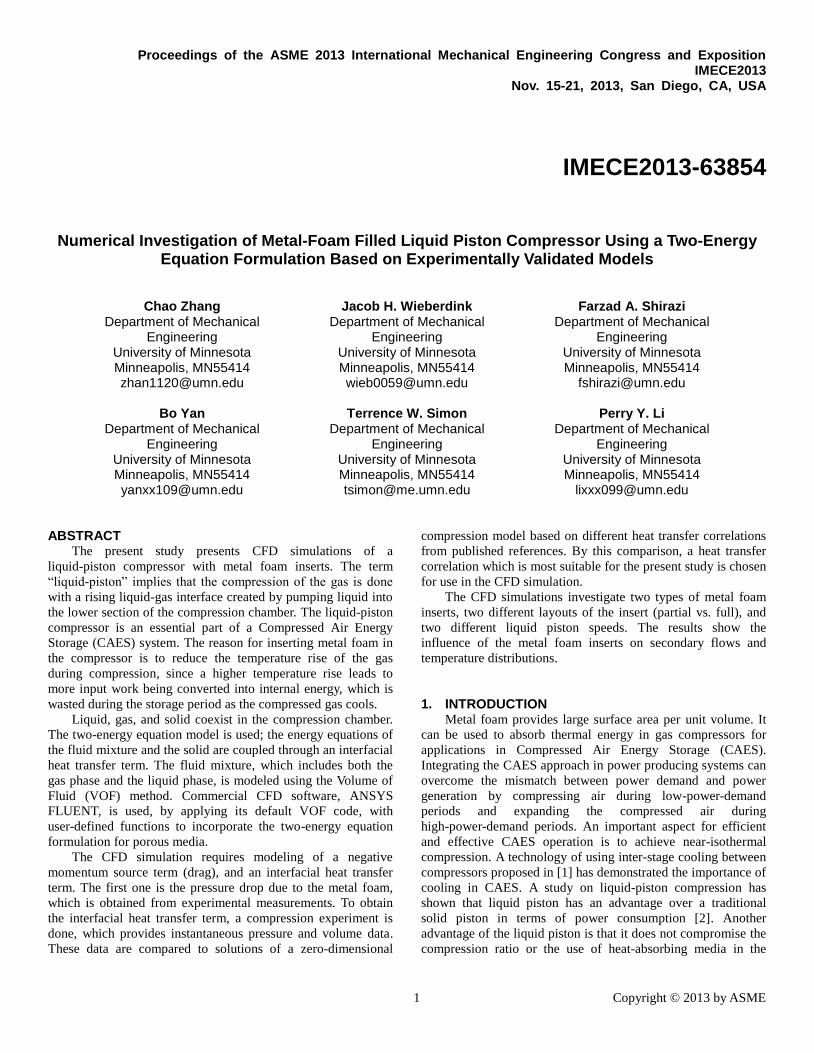
The computed and the experimentally measured air

temperature values are normalized based on the initial

temperature. The results are shown in Fig. 6. In the experiment,

the temperature is calculated from the ideal gas law, based on

instantaneous pressure and volume measurements. The

uncertainties of the initial volume and initial temperature

measurements are respectively 1.013𝑐𝑚3 and 0.8 K. The

uncertainties in the transient pressure and volume measurements

are, respectively, 1724Pa and 3𝑐𝑚3 . Using an uncertainty

propagation equation from [25] yields a temperature of 15 –

17K. Despite local mismatches and uncertainties in the

experiments, one sees from Fig. 6 that the solutions obtained

based on the Kamiuto and Yee correlation agree with

experimental measurements best throughout the whole

compression process. Therefore, the Kamiuto and Yee

correlation (Eq. (22)) is chosen for CFD modeling to calculate

interfacial heat transfer coefficients in Eqns. (7) and (12).

4. NUMERICAL METHOD, VERIFICATION, AND VALIDATION

4.1. Numerical Method

The transport equations, Eqns. (1) – (3), (7), and (12) are


solved by the finite volume method using the commercial CFD

Software ANSYS FLUENT including its VOF solver.

User-Defined-Function (UDF) codes are written to solve the

negative momentum source term, and the interfacial heat

transfer term based on the Kamiuto and Yee correlation is solved

for energy transport in the two-energy equation model. It is

assumed that the permeability and coefficient for the

Forchheimer term apply equally to water and air. The following

numerical methods are applied using ANSYS FLUENT. The 1st

order implicit method is used on the transient discretization.

Spatial derivatives of velocity, density, and temperature are

differenced using a 2nd

order upwind scheme. The algorithm of

Pressure Implicit with Splitting Operators [26] is used for

pressure-velocity coupling. The Pressure Staggering Option

scheme [27] is used for calculating discretized pressure values

on a staggered grid. The gradient terms are handled using the

Green-Gauss Cell-Based method, which calculates the face

value of a variable based on the arithmetic average of the values

at its adjacent cell centers. In each time step, convergence is

satisfied when the residual is smaller than 10−9. Eight CFD

runs are calculated by varying the inlet water velocity, the layout

of the insert (full-insert vs. partial-insert), and the pore size. The

cases are shown in Table 4. The schematic of the chamber is

shown in Fig. 2. In all cases, the dimensions of the chamber are:

𝐿 = 0.2 𝑚, 𝑅 = 0.025 𝑚. For the four full-insert cases, the

entire chamber length 𝐿 is occupied by the insert. For the four

partial-insert cases, the insert length is: 𝐿𝑖𝑛𝑠 =𝐿

2= 0.1 𝑚 ,

and the distance between the top boundary of the insert and the

top cap of the chamber is: 𝐿1 = 0.013 . The initial

temperature (for both fluid and solid) and pressure are: 297K

and 101644Pa. The initial air velocity is 0.0, and air volume

fraction is 1.0 in the chamber. The physical properties given in

Table 3 are used. The number of grid cells is 26,000 for the

full-insert cases, and 44,485 for the partial-insert cases. The time

step size is 0.0002s for the full insert cases with the smaller inlet

velocity. The time step size decreases as the number of nodes

and the velocity increase.

4.2. Grid-Independence Verification

CFD Run1, which has a relatively small number of grid

cells and large time step size compared to other runs, is tested

for grid independence. The grid-independence run is done on the

mesh that has 65,600 cells, using a time step size of 0.0001s.The

average air pressure and temperature at the final compression

time calculated from Run1 and its grid-independence run are,

respectively: 1,317,934Pa and 1,318,324Pa, and 345.8K and

345.6K. The temperature contour plots of the two at the final

compression time also display identical features. Therefore, grid

independence is satisfied.

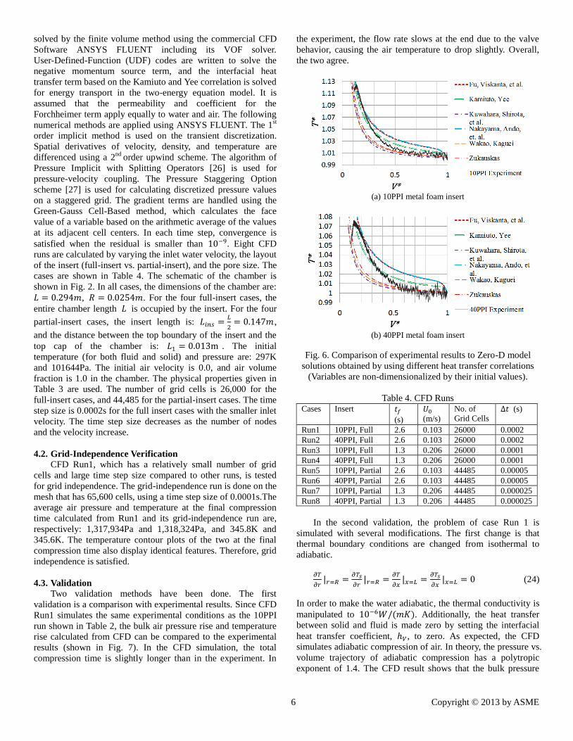
4.3. Validation

Two validation methods have been done. The first

validation is a comparison with experimental results. Since CFD

Run1 simulates the same experimental conditions as the 10PPI

run shown in Table 2, the bulk air pressure rise and temperature

rise calculated from CFD can be compared to the experimental

results (shown in Fig. 7). In the CFD simulation, the total

compression time is slightly longer than in the experiment. In

the experiment, the flow rate slows at the end due to the valve

behavior, causing the air temperature to drop slightly. Overall,

the two agree.

(a) 10PPI metal foam insert

(b) 40PPI metal foam insert

Fig. 6. Comparison of experimental results to Zero-D model

solutions obtained by using different heat transfer correlations

(Variables are non-dimensionalized by their initial values).

Table 4. CFD Runs Cases Insert 𝑡𝑓

(s)

(m/s)

No. of

Grid Cells 𝑡 (s)

Run1 10PPI, Full 2.6 0.103 26000 0.0002

Run2 40PPI, Full 2.6 0.103 26000 0.0002

Run3 10PPI, Full 1.3 0.206 26000 0.0001

Run4 40PPI, Full 1.3 0.206 26000 0.0001

Run5 10PPI, Partial 2.6 0.103 44485 0.00005

Run6 40PPI, Partial 2.6 0.103 44485 0.00005

Run7 10PPI, Partial 1.3 0.206 44485 0.000025

Run8 40PPI, Partial 1.3 0.206 44485 0.000025

In the second validation, the problem of case Run 1 is

simulated with several modifications. The first change is that

thermal boundary conditions are changed from isothermal to

adiabatic.

𝜕𝑇

𝜕 | 𝑅 =

𝜕𝑇𝑠

𝜕 | 𝑅 =

𝜕𝑇

𝜕𝑥|𝑥 𝐿 =

𝜕𝑇𝑠

𝜕𝑥|𝑥 𝐿 = 0 (24)

In order to make the water adiabatic, the thermal conductivity is

manipulated to 10−6 (𝑚𝐾). Additionally, the heat transfer

between solid and fluid is made zero by setting the interfacial

heat transfer coefficient, ℎ𝑉, to zero. As expected, the CFD

simulates adiabatic compression of air. In theory, the pressure vs.

volume trajectory of adiabatic compression has a polytropic

exponent of 1.4. The CFD result shows that the bulk pressure


verse volume follows the same adiabatic trend as shown in Fig.

8. At the end of compression, the pressure calculated from CFD

is slightly smaller than that from the theory. This is because the

liquid piston still conducts a small amount of heat for its

conductivity is not exactly made to zero for numerical stability

reasons.

(a) Pressure vs. time

(b) Temperature vs. time

Fig. 7. Experimental validation of CFD Run1

Fig. 8. Validation of CFD using adiabatic compression

No entries in the literature were found that simulate liquid

piston compression with porous media inserts. The closest

reference, to the best knowledge of the authors, is a solid piston

compression problem with partial insert of porous media [20];

yet, this paper formulates the problem with a one-energy

equation model and single phase flow. No pressure drop data are

given.

5. CFD RESULTS The eight CFD cases in Table 4 are simulated. The bulk air

temperature during compression is calculated and shown in Fig.

9. In most cases, the metal foam does a good job of supressing

the air temperature rise during compression. The smallest bulk

air temperature rise during compression is 35K (Run2), which is

compressed by the smaller liquid-piston speed and has a

chamber that is fully occupied by the finer-mesh metal foam.

For the same porous insert, higher compression speeds result in

larger temperature rises. For the same compression speed, the

full insert case has an advatage over the partial insert case, and

40PPI foam has an advantage over the 10PPI foam for reducing

the temperature rise. In the partial insert situations, since the

foam is inserted in the upper half of the chamber region, the

bulk air temperature rises fast in the beginning. As the air is

being pushed from the non-porous region into the porous region,

its temperature cools due to heat transfer with the metal foam.

This causes the bulk air temperature to drop by a few degrees in

the middle of the compression process.

(a) Water inlet velocity: 0.103m/s

(b) Water inlet velocity: 0.206m/s

Fig. 9. Air temperature rise during compression

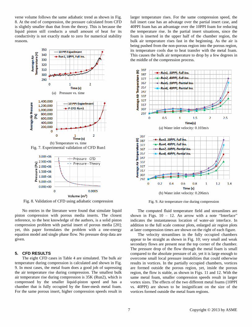
The computed fluid temperature field and streamlines are

shown in Figs. 10 – 12. An arrow with a note “Interface”

indicates the instantaneous location of water-air interface. In

addition to the full scale contour plots, enlarged air region plots

at later compression times are shown on the right of each figure.

The velocity streamlines in the fully occupied chambers

appear to be straight as shown in Fig. 10; very small and weak

secondary flows are present near the top corner of the chamber.

The pressure drop of the flow through the metal foam is small

compared to the absolute pressure of air, yet it is large enough to

overcome small local pressure instabilities that could otherwise

results in vortices. In the partially occupied chambers, vortices

are formed outside the porous region, yet, inside the porous

region, the flow is stable, as shown in Figs. 11 and 12. With the

same metal foam, smaller compression speeds result in larger

vortex sizes. The effects of the two different metal foams (10PPI

vs. 40PPI) are shown to be insignificant on the size of the

vortices formed outside the metal foam regions.


(a) Run1, 10PPI, Full Insert, = 0.103𝑚 , 𝑡𝑓 = 2.6

(b) Run2, 40PPI, Full Insert, = 0.103𝑚 , 𝑡𝑓 = 2.6

(c) Run3, 10PPI, Full Insert, = 0.206𝑚 , 𝑡𝑓 = 1.3

(d) Run4, 40PPI, Full Insert, = 0.206𝑚 , 𝑡𝑓 = 1.3

Fig. 10. Temperature field and velocity streamline at different times during compression, fully occupied chambers

At the end of compression, the air temperature distribution

becomes highly non-uniform, as volume decreases. Relatively

high local temperature values are seen in regions very close to

the top cap. In fully-occupied chambers, the high local air

temperature values at the end of compression are mainly due to

the stagnant flow. Since Nusselt numbers between the flow and

the porous medium depend on Reynolds number, stagnant flow

impedes heat transfer. In partially occupied chambers, the high

local air temperature values at the end of compression are high

due to lack of heat transfer surfaces; even though, the local flow

is relatively active, as shown by a vortex that has been formed

since the earlier stage of compression.

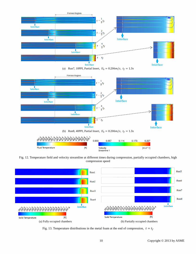
The computed solid temperature fields at the end of

compression for various cases are shown in Fig. 13. In the fully

occupied chambers, the largest local temperature rise in the solid

is less than 1K. In the partially occupied chambers, the largest

local temperature rise is 57.4K, which occurs at the top surface

of the metal foam. The bulk of the solid material is maintained

at a low temperature. Great differences in local temperature

values between the air and the solid are found in certain regions.

This confirms the advantage of using the two-energy equation

formulation instead of the one-energy, equilibrium formulation

for this kind of problem.

6. CONCLUSIONS The present study has numerically investigated liquid

piston compression chambers with metal foam inserts. Two

aluminum foams, 10PPI and 40PPI, are studied. The

permeability and the coefficient for the Forchheimer term are

obtained by measuring the pressure drop values. Compression

experiments using a liquid piston and metal foam inserts are

conducted to provide data which are compared to Zero-D

solutions based on different heat transfer correlations from

references. From the comparison, the Kamiuto and Yee heat

transfer correlation is found to be more suitable for the metal


`

(a) Run5, 10PPI, Partial Insert, = 0.103𝑚 , 𝑡𝑓 = 2.6

(b) Run6, 40PPI, Partial Insert, = 0.103𝑚 , 𝑡𝑓 = 2.6

Fig. 11. Temperature field and velocity streamline at different times during compression, partially occupied chambers, low

compression speed

foam and flow situations of the present study.

Based on the models validated by experiments, CFD

simulations on the compressor are done by combining the VOF

and the two-energy equation formulations. Fluid field and

temperature distributions are obtained from the CFD. The air

flow in the fully-occupied chamber is straight, parallel to the

chamber’s axial direction due to resistance of metal foam. In the

partially occupied chambers, secondary flow structures are

present during compression in the air regions outside the metal

foam. The dimensions of vortices generated are related to

compression speed; smaller speeds induce larger vortices, and

larger speeds induce smaller vortices. The air is most effectively

cooled in fully occupied chambers. The temperature

distributions of the metal foam in the partially occupied

chambers are non-uniform at the end of compression. High

temperature values are found at the top surface of the metal

foam. In fully occupied chambers, the maximum local

temperature rise for the metal foam is less than 1K. The very

different local temperatures between the metal foam and the

adjacent fluid confirms the appropriateness of using the

two-energy equation modeling (instead of the one-energy

equation, equilibrium modeling) for CFD simulations of flow

being compressed through porous media.

The formation of vortical structures is enhanced when a

partial insert is used. These vortical structures have the potential

to reduce the maximum air temperature by mixing the stagnant

high temperature air at the top of the chamber with the relatively

cool air near the walls and porous insert. This study shows that,

although vortical structures are enhanced when a partial insert is

used, the maximum air temperature is still higher than the full

insert case. This suggests that an optimum 𝐿1 distance may

exist such that mixing is enhanced without diminishing too

much the heat-absorbing solid surface. This could be

investigated in future studies.


(a) Run7, 10PPI, Partial Insert, = 0.206𝑚 , 𝑡𝑓 = 1.3

(b) Run8, 40PPI, Partial Insert, = 0.206𝑚 , 𝑡𝑓 = 1.3

Fig. 12. Temperature field and velocity streamline at different times during compression, partially occupied chambers, high

compression speed

(a) Fully occupied chambers (b) Partially occupied chambers

Fig. 13. Temperature distributions in the metal foam at the end of compression, 𝑡 = 𝑡𝑓


NOMENCLATURE

𝑎𝑉 Area per unit volume of porous medium

𝑏 Coefficient for the Forchheimer term

𝑐𝑝 Constant-pressure specific heat

𝑐 Constant-volume specific heat

𝑑 A characteristic length based on filament diameter

𝑑𝑓 Filament diameter

𝑑𝑚 Mean pore diameter

𝑔 Gravitational acceleration

ℎ𝑠𝑓 Surface heat transfer coefficient

ℎ𝑉 Volumetric heat transfer coefficient

𝐾 Permeability

𝑘 Thermal conductivity

𝐿 Chamber length

𝐿1 Length of the upper region without insert

𝐿𝑖𝑛𝑠 Length of the insert region

𝑁𝑢 Nusselt number

𝑃 Average pressure

𝑝 Local pressure

𝑃𝑟 Prandtl number

𝑅 Radius of chamber

𝑟 Radial coordinate

ℛ Ideal gas constant

𝑅𝑒𝑑 Reynolds number based on characteristic length 𝑑

𝑆 𝑚 Momentum source term

𝑇 Local air temperature

𝑇 Initial temperature; wall temperature

𝑇𝑎𝑖 Average air temperature in the chamber

𝑇 Local solid temperature

𝑇𝑠𝑜𝑙𝑖𝑑 Average temperature of solidin the chamber

𝑡 Time

𝑖𝑛 Liquid piston velocity

𝑉 Instantaneous volume of chamber

𝑥 Axial coordinate

Greek Symbols

𝛼 Volume fraction

𝜖 Porosity

𝜇 Dynamic viscosity

𝜌 Density

Subscripts

0 Initial value of variable

1 Air phase

2 Water phase

Darcian velocity

Values at the end of compression

Solid

Superscripts

dimensionless variable

ACKNOWLEDGEMENTS This work is supported by the National Science Foundation

under grant NSF-EFRI #1038294, and University of Minnesota,

Institute for Renewable Energy and Environment (IREE) under

grant: RS-0027-11. The authors would like to thank also the

Minnesota Super Computing Institute for the computational

resources used in this work.

REFERENCE 1. M. Nakhamkin, M. Chiruvolu, M. Patel, S. Byrd, R.

Schainker, “Second Generation of CAES Technology –

Performance, Operations, Economics, Renewable Load

Management, Green Energy,” POWER_GEN International

Conference, Vas Vegas, NV, Dec. 2009

2. J. Van de Ven and P. Y. Li, “Liquid Piston Gas

Compression,” Applied Energy, v. 86, n. 10, pp. 2183-2191,

2009

3. P. Y. Li, E. Loth, T. W. Simon, J. D. Van de Ven, and S. E.

Crane, “Compressed Air Energy Storage for Offshore Wind

Turbines,” 2011 International Fluid Power Exhibition

(IFPE), Las Vegas, NV, March, 2011

4. C. Zhang, T. W. Simon, P. Y. Li, “Storage Power and

Efficiency Analysis Based on CFD for Air Compressors

Used for Compressed Air Energy Storage,” Proceedings of

ASME 2012 International Mechanical Engineering

Congress & Exposition, Houston, TX, Nov. 2012

5. P. Mane, A. Dasare, G. Deshmukh, P. Bhuyar, K. Deshmukh,

and A. Barve, “Numerical Analysis of Pulse Tube

Cryocooler,” International Journal of Innovative Research

in Science, Engineering, and Technology, Vol. 2, Issue 3,

Mar. 2013

6. P. Karuppusamy and R. Senthil, “Design, Analysis of Flow

Characteristics of Catalytic Converter and Effects of Back

Pressure on Engine Performance,” International Journal of

Research in Engineering & Advanced Technology, Vol. 1,

Issue 1, Mar. 2013

7. G. Zaragoza, and R. Goodall, “Metal Foams with Graded

Pore Size for Heat Transfer Applications,” Advanced

Engineering Material, Vol. 15, No. 3, pp. 123-128, 2013

8. Chin-Tsau Hsu, “Dynamic Modeling of Convective Heat

Transfer in Porous Media,” in: K. Vafai (editor), Handbook

of Porous Media (2nd Edition), Taylor and Fracis Group,

LLC, 2000

9. K. Vafai, C. L. Tien, “Boundary and Inertial Effects on

Flow and Heat Transfer in Porous Media,” Int. J. Heat Mass

Transfer, Vol. 24, pp. 195-203, 1981

10. M. Sozen, and T. Kuzay, “Enhanced Heat Transfer in Round

Tubes with Porous Inserts,” Int. J. Heat and Fluid Flow, Vol.

17, pp. 124-129, 1996

11. N. Wakao, and S. Kaguei, “Heat and Mass Transfer in

Packed Beds,” Gorden and Breach, pp. 243-295, New York,

1982

12. F. Kuwahara, M. Shirota, and A. Nakayama, “A Numerical

Study of Interfacial Convective Heat Transfer Coefficient in

Two-Energy Equation Model for Convection in Porous

Media,” In.t J. Heat Mass Transfer, Vol. 44, pp. 1153-1159,

2001

13. A. A. Zukauskas, “Convective Heat Transfer in Cross-Flow,”

in: S. Kakac, R. K. Shah, and W. Aung (Editors), Handbook

of Single-Phase Convective Heat Transfer, Wiley, New

York, 1987

14. A. Nakayama, K. Ando, C. Yang, Y. Sano, F. Kuwahara,

and J. Liu, “A Study on Interstitial Heat Transfer in


Consolidated and Unconsolidated Porous Media,” Heat and

Mass Transfer, Vol. 45, No. 11, pp. 1365-1372, 2009

15. K. Kamiuto, and S. S. Yee, “Heat Transfer Correlations for

Open-Cellular Porous Materials,” Int. Comm. Heat Mass

Transfer, Vol. 32, pp. 947-953, 2005

16. W. Lu, C. Y. Zhao, and S. A. Tassou, “Thermal Analysis on

Metal-Foam Filled Heat Exchangers. Part I: Metal-Foam

Filled Pipes,” Int. J. Heat Mass Transfer, Vol. 49, pp.

2751-2761, 2006

17. M. B. Saito, and M. J.S. de Lemos, “Laminar Heat Transfer

in a Porous Channel Simulated with a Two-Energy

Equations Model,” International Communications in Heat

and Mass Transfer, Vol. 36, pp. 1002-1007, 2009

18. Y. P. Du, Z. G. Qu, C. Y. Zhao, and W. Q. Tao, “Numerical

Study of Conjugated Heat Transfer in Metal Foam Filled

Double-Pipe,” Int. J. Heat Mass Transfer, Vol. 53, pp.

4899-4907, 2010

19. C. Xu, Z. Song, L. Chen, Y. Zhen, “Numerical Investigation

on Porous Media Heat Transfer in a Solar Tower Receiver,”

Renewable Energy, Vol. 36, pp. 1138-1144, 2011.

20. N. Zahi, A. Boughamoura, H. Dhahri, and S Ben Nasrallah,

“Flow and Heat Transfer in a Cylinder with a Porous Insert

along the Compression Stroke,” Journal of Porous Media,

Vol. 11 (6), pp. 525-540, 2008

21. C. W. Hirt, and B. D. Nichols, “Volume of Fluid (VOF)

Method for Dynamics of Free Boundaries,” Journal of

Computational Physics, vol 39, pp. 201-225, 1981

22. A. Q. Raeini, M. J. Blunt, and B. Bijeljic, “Modeling

Two-Phase Flow in Porous Media at the Pore Scale Using

the Volume-of-Fluid Method,” Journal of Computational

Physics, Vol. 231, pp. 5653-5668, 2012

23. C. Zhang, F. A. Shirazi, B. Yan, T. W. Simon, P. Y. Li, and J.

Van de Ven, “Design of an Interrupted-Plate Heat

Exchanger Used in a Liquid-Piston Compression Chamber

for Compressed Air Energy Storage,” Proceedings of

ASME 2013 Summer Heat Transfer Conference,

Minneapolis, MN, July 2013

24. “Air Properties,” <URL:

http://www.engineeringtoolbox.com/air-properties-d_156.ht

ml>, (Accessed Apr. 2013)

25. S. J. Kline, and F. A. McClintock, “Describing

Uncertainties in Single-Sample Experiments,” Mechanical

Engineering, Vol. 75, pp. 3-8, Jan. 1953

26. R. I. Issa, “Solution of implicitly discretized fluid flow

equations by operator-splitting,” J. Comp. Phys. Vol. 62, pp.

40-65, 1986

27. S. V. Patankar, Numerical Heat Transfer and Fluid Flow.

Hemisphere, Washington, DC, 1980.

Documents

IMECE2013-63854 - Semantic Scholar€¦ · IMECE2013-63854 Numerical ... liquid-piston compressor with inserted metal foam are done in the present study. The volume-averaging technique