Imitation and Belief Learning in an Oligopoly Experimentpeople.exeter.ac.uk/dgbalken/EE08/Offermann.pdf · imitation, we hypothesize this treatment to be relatively favourable for

Review of Economic Studies (2002)69, 973–997 0034-6527/02/00380973$02.00c© 2002 The Review of Economic Studies Limited

Imitation and Belief Learning in anOligopoly Experiment

THEO OFFERMANUniversity of Amsterdam

JAN POTTERSTilburg University

and

JOEP SONNEMANSUniversity of Amsterdam

First version received September1998; final version accepted November2001(Eds.)

We examine the force of three types of behavioural dynamics in quantity-setting triopolyexperiments: (1) mimicking the successful firm, (2) rules based on following the exemplary firm, and(3) rules based on belief learning. Theoretically, these three types of rules lead to the competitive, thecollusive, and the Cournot–Nash outcome, respectively. In the experiment we employ three informationtreatments, each of which is hypothesized to be conducive to the force of one of the three dynamicrules. To a large extent, the results are consistent with the hypothesized relationships between treatments,behavioural rules, and outcomes.

1. INTRODUCTION

Although quantity-setting oligopoly is one of the “workhorse models” of industrial organization(Martin, 1993), empirically there is much ambiguity about its outcome. A recent survey bySlade (1994) indicates that most empirical studies reject the hypothesis that the outcome isin line with the Cournot–Nash equilibrium of the corresponding one-shot game. Interestingly,however, outcomes on both sides of the Cournot–Nash outcome are found. In the experimentalliterature, a similar state of affairs obtains. Many experimental oligopoly games result in higherthan Cournot–Nash production levels, some result in lower production levels (Holt, 1995).

Theoretically, three main benchmarks for the quantity setting oligopoly game exist: theWalrasian equilibrium, where each firm’s profits are maximized given the market clearingprice; the Cournot–Nash equilibrium, where each firm’s profits are maximized given the otherfirms’ quantity choices; and the collusive outcome, where aggregate profits are maximized. Tomotivate these benchmarks, one may search for dynamic underpinnings of these benchmarks.1

In this paper we present an experimental investigation of such dynamic underpinnings based on

1. For other stylized games it is often shown that learning may play a decisive role in the process of equilibriumselection (e.g.Brandts and Holt (1992), Van Huyck, Batallio and Beil (1990)).

973

974 REVIEW OF ECONOMIC STUDIES

belief learning and imitation. Both belief learning and imitation have received support in otherexperimental settings.2,3

In principle, players could spend effort to find the Cournot–Nash equilibrium of the gameand play accordingly. Decision costs may prevent them from doing so, however. Given thatit is costly to derive best response strategies and to deduce the corresponding equilibrium, itmay be reasonable to assume that players look for strategies that save on cognitive effort anddecision costs.4 Deviations from best response behaviour could thus explain the deviations fromthe Cournot–Nash outcome that are observed in empirical and experimental work.

A starting point for our study is a result by Vega-Redondo (1997) on the effect of a rulebased on imitation in symmetric oligopoly. He shows that if firms tend to mimic the quantitychoice of the most successful firm, then there will be a tendency for the industry to evolve towardthe competitive outcome. The successful firm is the firm with the highest profit. Typically, thisfirm produces a higher quantity than the other firms. This approach thus provides a dynamicbehavioural underpinning for Walrasian equilibrium.

The result is counter-intuitive in some sense. By imitating the choice of the most profitablefirm, the industry as a whole develops toward a very unprofitable outcome. Therefore, assuggested by Sinclair (1990), in the presence of a partial conflict between individual and groupinterest, it may be reasonable for imitators to follow the “saint” rather than to mimic the “villain”.In the social psychological literature, it is also common to hypothesize that cooperative oraltruistic acts serve as examples for others (Bandura (1986), Sarason, Sarason, Pierce and Shearin(1991)). In the oligopoly game, the “exemplary firm” produces the quantity that, if followed byall firms, leads to higher profits than following any of the other firms. The exemplary firm istypically the firm that produces the lowest quantity. We will consider three rules in the “followingclass”, which all propose that the non-exemplary firms choose the exemplary quantity. Theserules differ (only) in the degree to which the exemplary firm conditions its choices on those ofthe non-exemplary firms. As will be shown in the next section, the industry will evolve towardthe collusive outcome when firms use either of these rules from the following class.

The belief learning approach provides a completely different underpinning of behaviour.According to this approach firms form beliefs about the choices of other firms on the basis ofthe assumption that the history of the game provides information about the future. Given theirbeliefs firms myopically choose the quantity with the highest expected profits. For some marketstructures, like the one we implement in this paper, both best response learning and fictitious playconverge to the Cournot–Nash equilibrium independent of initial play.

Hence, each of the three benchmarks in the quantity-setting oligopoly can be foundedon a different behavioural rule. How can the theoretical results be reconciled with the widerange of empirical findings? As Shubik (1975) notes, “. . . the specific details of communication,information, and the mechanisms of the market have considerable influence on the play whennumbers are few”. It may be that specific details of the environment trigger a specific dynamic

2. For experimental work on belief learning see Boylan and El-Gamal (1993), Cheung and Friedman (1997),El-Gamal, McKelvey and Palfrey (1994), Mookherjee and Sopher (1994) and Offerman, Schram and Sonnemans (1998).Experimental work on imitation focuses on the role of imitation in decision tasks, see Offerman and Sonnemans (1998)and Pingle (1995). Of course, there are other dynamic rules—such as reinforcement learning (Roth and Erev, 1995)—thathave found experimental support, but here we focus on imitation and belief learning.

3. The discussion about the appropriateness of the three benchmarks has long centred around the so-calledconjectural variations. An advantage of this approach is that it encompasses all three benchmarks within a unifiedframework. A problem, however, is that conjectures are used to reflect the manner in which firms react to each others’choices, whereas the models are essentially static in nature (Daughety, 1985). As suggested by Fraser (1994), it wouldbe worthwhile to search for dynamic underpinnings of particular conjectures.

4. There is a growing awareness in both empirical and theoretical work that decision costs are a relevant ingredientof decision making (e.g.Abreu and Rubinstein (1988), Conlisk (1980, 1988, 1996), Ho and Weigelt (1996), Pingle andDay (1996), Rosenthal (1993)).

OFFERMANET AL. IMITATION AND BELIEF LEARNING 975

rule of behaviour, and that a specific dynamic rule leads to a specific benchmark. In particular,the type of feedback about the choices and performance of other firms may affect the decisioncosts and hence the use of alternative strategies. Some feedback may be conducive to mimickingthe most successful firm and may direct the industry toward the Walrasian equilibrium. Otherfeedback may be conducive to following the exemplary firm or to belief learning and thuslead to the collusive or the Cournot–Nash outcome, respectively. Experimental research has theimportant advantage that the type of feedback can be precisely controlled. Thus the force of thispotential explanation for the range of empirical findings can be examined. Such an examinationis the main goal of our paper.

For imitation to be possible, firms need information about the quantity chosen by each otherfirm. Without fully individualized feedback about quantities, firms are unable to detect the choiceof either the successful firm or the exemplary firm. This simple observation leads to the base-linetreatment of our experiment. In this treatment the information that firms receive about other firmsis restricted to the sum of the quantities produced in the previous period. We refer to this treatmentas treatmentQ (Q is mnemonic for aggregate information). By excluding the possibility ofimitation, we hypothesize this treatment to be relatively favourable for belief learning.

In the other two treatments we provide more feedback information than in treatmentQ. Thismay stimulate the employment of rules based on imitation which are cognitively less demandingthan belief learning. In treatmentQqπ , firms receive individualized feedback information onboth quantities and profits (q is a mnemonic for individualized quantity information andπ forprofit). This information makes comparative profit appraisals available at minimal decision cost.Therefore, we hypothesize this treatment to be relatively favourable for mimicking the successfulfirm.

In treatmentQq firms receive individualized information about quantities but not aboutprofits. So, players can imitate but it will not be obvious whom to imitate. Mimicking the success-ful firm is no longer for free and requires some costly deliberations. Thus, relative to treatmentQqπ , we hypothesize that treatmentQq encourages the use of rules based on the following.5

In a related paper, Huck, Normann and Oechssler (1999) independently examine the role ofimitation in an experimental quantity setting oligopoly game. The emphasis of their paper is onthe impact of informationprior to the experiment, while our paper is primarily concerned withthe impact of feedback information providedduring the experiment. In the concluding section,we will explain how the results of Hucket al. complement ours.

The remainder of the paper is organized as follows. The next section presents the institutionsof the market and presents the theoretical results. Section 3 describes the design and procedure ofthe experiment. Section 4 elaborates on the hypothesized relation between feedback informationand dynamic rule of conduct. Section 5 presents the results and, finally, Section 6 provides aconcluding discussion.

2. MARKET AND THEORY

In our marketn firms produce a homogeneous commodity. Firms face identical cost functions:

C(qi ) = cq3/2i ,

wherec denotes a given cost parameter andqi denotes the quantity produced by firmi (1 ≤ i ≤

n). The inverse demand function is

P(Q) = a − b√

Q; Q =

∑n

i =1qi ,

5. The availability and dissemination of information about the actions of individual members of an industry havealso been a matter of some concern to antitrust authorities (Scherer and Ross, 1990, Chapter 9). It is feared that “tacitcollusion” is easier when other members can be closely monitored and, if necessary, punished.


TABLE 1

Benchmarks of the game

Quantities of three firms Price Profits of three firmsBenchmark qi (i = 1, 2, 3) P(Q) πi (i = 1, 2, 3)

Walrasian equilibrium 100 15 500Collusive outcome:

(a) real quantities 56·25 22·5 843·75(b) integer quantities 56 22·55 843·74

Cournot–Nash equilibrium 81 18 729

wherea andb denote given demand parameters.The three benchmarks for this game are defined as follows. First, the Walrasian equilibrium

is obtained if and only if each firm produces quantityqw:

P(nqw)qw− C(qw) ≥ P(nqw)q − C(q), ∀q ≥ 0;

⇒ qw=

4a2(2b

√n + 3c

)2.

Second, the collusive outcome is reached if and only if each firm produces quantityqc:

P(nqc)qc− C(qc) ≥ P(nq)q − C(q), ∀q ≥ 0;

⇒ qc=

4a2(3b

√n + 3c

)2.

Third, the Cournot–Nash equilibrium is reached if and only if each firm produces quantityqN :

P(nqN)qN− C(qN) ≥ P((n − 1)qN

+ q)q − C(q), ∀q ≥ 0;

⇒ qN=

4a2(b(2n+1)√

n+ 3c

)2.

In the experiment we chosen = 3, c = 1, a = 45 andb =√

3. For each of the threetheoretical benchmarks Table 1 shows the corresponding values of quantities, prices and profits.6

For the remainder of the paper we will restrict our attention to the case where three firms interactrepeatedly from periodt = 1, 2, . . . onward in a stationary environment.

The first dynamic rule that we examine hypothesizes that firms mimic the choice of the firmthat was most successful in the previous period. Besides an imitation part, the rule consists of anexperimentation (randomization) part. We will say that a firm “mimics the successful firm” if itexperiments with probabilityε and it imitates the successful firm with probability(1− ε). When

6. The following considerations played a role for the choice of functional forms and parameter values. First,if we wish to allow for both “mimicking the successful firm” and “following” at least three firms should be present.Moreover, with three firms in the industry it is easy to conclude whether a change in the output of the firm with theintermediate production level is better organized by the model that predicts that this firm mimics the successful firm orby a model from the following class. With more than three firms it might be less clear whether a firm with an intermediateproduction level imitates one of the successful or exemplary firms, or whether it imitates yet another firm. Second, wewanted to ensure that even at the Walrasian equilibrium subjects made positive profits. Therefore we chosec > 0. Toprevent subjects from making losses, we restricted the production set of each firm to (integer) values of the interval [40,125]. Third, we wanted to separate the benchmarks as much as possible. At the same time we wanted the differencebetween the Walrasian quantity and the Cournot–Nash quantity to be more or less equal to the difference between theCournot–Nash quantity and the collusive quantity. Finally, we wanted to employ an environment in which both fictitiousplay and best-response dynamics (“Cournot learning”) would converge to the Cournot–Nash equilibrium. This impliedthat we could not use a purely linear specification (see Theocharis (1960)).


a firm experiments, it chooses some arbitrary quantity level from the feasible set.7 When a firmimitates the successful firm, it chooses the same quantity as was produced by the firm (or one ofthe firms) with the highest profit in the previous period. The successful firm imitates by repeatingits former choice.

Result 1. If all firms mimic the successful firm, the unique stochastically stable state ofthe process is(qw, . . . , qw) asε → 0.

Result 1 is due to Vega-Redondo (1997).8 Sketches of the proofs of the results in this sectionare provided in Appendix A. The result indicates that in the long run, only the Walrasian outcomewill be observed a significant fraction of the time. The intuition is as follows. Assume that firmsproduce different quantities. If the price is above the marginal costs of the high quantity firm, thiswill be the firm with the highest profit. Imitation then induces the other firms to select this highquantity in the next period. The firms remain at this symmetric, say sub-Walrasian, allocationuntil one of the firms experiments. If this firm selects a lower quantity, it will earn a lower profitand will return to the other firms in the next period. If, however, it selects a higher quantity itwill earn a higher profit (as long as price is above marginal cost) and will be mimicked by theother firms in the next period. Gradually this process moves toward the Walrasian outcome. TheWalrasian outcome is more robust than other symmetric outcomes, because a unilateral deviationby one firm will not be imitated by other firms.

The other rules based on imitation assume that firms follow the firm that sets the goodexample from the perspective of industry profit. The exemplary firm is the firm (one of thefirms) with the quantity that would give the highest sum of profits if it were followed by allfirms. All following rules considered here assume that the non-exemplary firms choose theexemplary quantity. Since following rules are not standard in the literature, we consider threevariations to this rule which differ in the degree to which the exemplary firm conditions itschoice on those of the non-exemplary firms. According to “follow the exemplary firm” rule theexemplary firm will continue to produce the same output as in the previous period. According to“follow and guide”, the exemplary chooses a quantity midway between its own previous choiceand that of the exemplary other firm, that is, the firm that is exemplary if its own choice isdisregarded. According to “follow exemplary other firm”, the exemplary firm follows the choiceof the exemplary other firm (just as the non-exemplary firms do). By conditioning its choice onthose of the other firms, the exemplary firm can protect itself from being exploited. By applyinga mild punishment, it can still send a signal to head toward a more cooperative outcome. Thedifferent rules strike a different balance between these two motivations.

Besides the following part, the rules consist of an experimentation part. We will say thata firm uses one of the following rules if it experiments with probabilityε and it chooses thepredicted quantity with probability(1 − ε).

Result 2. If firms choose a rule from the following class, the unique stochastically stablestate of the process is(qc, . . . , qc) asε → 0.

The intuition for the result is easy. After one round of following the non-exemplary firmswill follow the firm that was exemplary in the previous period. The exemplary firm itself mayhave moved away toward a higher quantity (under follow and guide or follow exemplary other),

7. Here and in what follows the Results 2 and 3, it is assumed that the probability that a firm experiments isindependent across players and time. Furthermore, if a firm experiments, it chooses a quantity level according to a givenstationary probability distribution with full support (see Vega-Redondo (1997), Young (1993)).

8. The result holds as long as there are identical cost functions and a decreasing demand function. Firms areassumed to choose from a common finite grid containing the Walrasian equilibrium. It is allowed that a firm does notchange its quantity with positive probability.


but the next round of following will bring it back to the quantity choices of the other two firms,who are now exemplary. Since the latter two firms are exemplary for each other, they will staywhere they are. From this symmetric outcome, they will only move away if one of the firmsexperiments and chooses a quantity which is closer to the collusive outcome. Eventually, thisprocess will lead to the collusive outcome.

An alternative dynamic approach hypothesizes that firms use belief learning processes toadapt their behaviour. Belief learners trust the stability in the choice pattern of others. Thesimplest version of belief learning is known as the Cournot rule or best response rule. Accordingto this rule each firm believes that the aggregate quantity produced by the other firms in theprevious period will be produced again in the present period. A firm best responds if it myopicallymaximizes its expected payoff. Fictitious play is another representative of the class of belieflearning models. This rule looks further back than one period only. According to an adaptedversion of fictitious play, each firm chooses a best response to the average aggregate quantityproduced by the other firms in all previous periods. In the remainder of the paper we will simplyrefer to fictitious play when we have this adapted version in mind.9

We supplement the belief learning rules with an experimentation part. A firm uses a rulefrom the belief learning class if it experiments with probabilityε and it chooses the predictedquantity with probability(1−ε). Belief learning does not generally converge toward the Cournot–Nash outcome in quantity-setting oligopoly games. Our oligopoly game is dominance solvable,however, which ensures that it does. Experimentation can occasionally take the outcome awayfrom Cournot–Nash, but if the experimentation probability is small the process will spend mostof its time at the equilibrium.

Result 3. If firms use a rule from the belief learning class, the unique stochastically stablestate of the process in the triopoly market described above is(qN, . . . , qN) asε → 0.

3. DESIGN AND PROCEDURES

Both the instructions and the experiment were computerized.10 A transcript of the instructions isprovided in Appendix B. Subjects could read the instructions at their own pace. It was explainedto subjects that they made decisions for their “own firm”, while two other subjects made thedecisions for “firm A” and “firm B”. It was also explained that they would interact with the sametwo other subjects for the whole experiment, but that they could not know the identity of thesetwo subjects. Subjects were also informed that the experiment would consist of 100 periods.11

Table 2 presents the main features of the three treatments. The design is “nested” in thesense that the treatments can be strictly ordered on the amount of information provided to thesubjects. In all treatments, the players received feedback information on total quantity, price,

9. According to the “true” version of fictitious play, firms believe that others select a quantity with probabilityequal to the observed empirical frequency of that quantity in past play. One has to make (rather arbitrary) assumptionsabout firms’ prior distribution before they enter the game. Given its updated beliefs a firm chooses the quantity that(myopically) maximizes its expected payoff. Because the production set of each player is rather large in the presentgame, fictitious play only becomes meaningful after a considerable length of play. Therefore, we consider an adaptedversion of fictitious play that is easier to implement.

10. The program is written in Turbo Pascal using the RatImage library. Abbink and Sadrieh (1995) providedocumentation of this library. The program is available from the authors.

11. The disadvantage of a known final period is that subjects may anticipate the end of the experiment andthen an end-effect may occur. The alternative is to try to induce an infinite horizon, but such a procedure has its owndisadvantages, especially on the point of credibility (see also, Selten, Mitzkewitz and Uhlig (1997)). A theoreticaladvantage of a known final period is that a unique subgame-perfect equilibrium exists for the repeated game. Furthermore,we chose for 100 periods because simulations indicated that this was about the time needed for all the dynamic rules(especially fictitious play) to converge to the corresponding benchmarks.


TABLE 2

Summary of treatments

Treatment Baseline information Additional information

Q Ri , Ci , πi , Q, P —Qq Ri , Ci , πi , Q, P qj , qk

Qqπ Ri , Ci , πi , Q, P qj , qk, π j , πk

Notes:all information concerns the previous period. Subscriptirefers to the firm itself; subscriptsj andk concern the othertwo firms in the industry.R denotes revenue;C denotes costs;π denotes profit;Q denotes aggregate production;P denotesprice.

private revenue, private cost and private profit. In fact, in treatmentQ this was all the informationthat players received in a particular period about the outcome of play in the previous period. IntreatmentQq, firms received additional information on the individual quantities produced by theother two firms. Finally, in treatmentQqπ , firms were not only provided with individualizedinformation about the quantities but also about the corresponding profits to the other two firms.This was the only point where the three treatmentsQ, Qq and Qqπ and their instructionsdiffered: the screen that popped up after a period had ended, contained different information(see Appendix B).

Each period, firms had to decide simultaneously how much to produce. They could onlychoose integer values between and including 40 and 125. It was emphasized that all firms hadsymmetric circumstances of production,i.e. all firms had the same cost function. All firms in anindustry received the same price for each commodity produced. Both the relationship betweenown production and costs and between aggregate production and price (cf. Section 2) wascommunicated to subjects in three ways: via a table, a figure and the formula. It was explainedthat all three forms contained exactly the same information, and that subjects could make useof the form that they liked best. Our impression is that most subjects used the tables. We alsoprojected the cost and price tables on the wall, in order to induce common knowledge of themarket structure. Copies of these forms of information will be sent on request.

We explained that a firm’s profit in a period was its revenue (own production× price) minusits costs. Although we provided a subject with the information about her profit after a period hadended, we did not provide profit tables.12 Neither did we give away best responses, as is donein some experiments. However, subjects were given regular calculators to reduce computationalproblems. Before the experiment started, subjects had to correctly answer some questions testingtheir understanding before they could proceed with the experiment.

A subject’s profits were added up for all 100 periods. During the experiment subjectsgenerated experimental points. At the end of the experiment the experimental points wereexchanged for Dutch guilders at an exchange rate of 1300 experimental points= 1 Hfl. Subjectsknew how points were converted into Dutch guildersbeforeplaying the game. The subjects filledin a questionnaire, asking for some background information, before they were privately paid theirearnings.

Subjects were recruited at the University of Amsterdam. A total of 102 subjects participated:33 subjects participated in treatmentQ, 36 subjects participated in treatmentQq and 33subjects participated in treatmentQqπ . Subjects had no prior experience with directly relatedexperiments, and, of course, subjects participated in the experiment only once. An experiment

12. Of course, subjects had all information necessary to construct such tables themselves if they wanted.


lasted between 1 1/2 and 2 h. Average earnings were 55·13 Hfl, which at the time was the Dutchequivalent of about U.S.$30.

4. HYPOTHESES

In this section we elaborate on the hypothesis that treatmentsQ, Qq andQqπ are conducive tothe employment of belief learning, following the exemplary firm, and mimicking the successfulfirm, respectively. Also we speculate on how the outcome will be affected if some players in thepopulation will behave more rationally.

First note that in all treatments a firm receives information about total production in theprevious period. In principle, it is therefore possible to behave in accordance with belief learningin each of the treatments. TreatmentQ is conducive to belief learning in the sense that it isthe only treatment where firms cannot imitate because they lack the necessary individualizedinformation to do so. As a result we expect that treatmentQ will be relatively favourable foroutcomes to move toward the Cournot–Nash outcome.

The hypothesis that collusive outcomes will be observed more often in treatmentQq thanin treatmentQ is based on the premise that individualized information on quantities may givefirms hints as to what the appropriate quantity may be. Unlike in treatmentQ, firms have thepossibility to employ either unconditional or conditional rules that aim to identify and follow theexemplary firm. This treatment may especially foster the use of the more plausible conditionalfollowing rules, as the individualized quantity information allows firms to send and read signalsmore effectively, thereby decreasing the likelihood that they will be unilaterally exploited. Forexample, even a small reduction or increase in quantity can be detected as such by other players,whereas this is much more difficult when players receive only aggregate quantity information. Asa consequence, we expect relatively more behavioural strategies aiming for the collusive outcomein treatmentQq than in treatmentQ.13

Information-wise, treatmentsQq andQqπ are similar in the sense that fully rational agentsin treatmentQq could compute the extra information about rivals’ profits that is provided intreatmentQqπ . Hence, technically speaking, rules based on following as well as mimicking thesuccessful firm can be applied in both treatmentQqπ and treatmentQq. However, the cognitiveeffort required to apply these rules differs between treatmentQq and treatmentQqπ . Mimickingthe successful firm is a decision rule that can be employed at minimal decision costs in treatmentQqπ . Agents receive the information needed for a comparison of profits on a silver plate. IntreatmentQq, agents could also mimic the successful firm, but here they would have to spendconsiderable effort in identifying the successful firm. At the same time, rules based on followingare equally costly in treatmentQq and treatmentQqπ . In both treatments, firms can detect theexemplary firm at the same cognitive effort. To the extent that it is more natural to evaluateprofits at symmetric quantity choices than at asymmetric choices, determining the exemplaryfirm is cognitively less demanding in treatmentQq than finding the successful firm. Hence, interms of relative decision costs, treatmentQq is conducive to following and treatmentQqπ tomimicking. As a result, we expect the collusive (Walrasian) outcome to have a relatively strongattraction in treatmentQq (treatmentQqπ ).

For the theoretical results 1–3 it is assumed that all players follow a specific adaptive rulewhich is different for each of the three treatments. This assumption provides clear benchmarkresults, but it seems too extreme to have descriptive relevance. What may be reasonably

13. In a public goods experiment, Sell and Wilson (1991) find that the provision of individualized information oncontribution levels allows subjects to achieve higher levels of cooperation than in case feedback is restricted to aggregatecontributions. This result is in line with our hypothesis about the effect of individualized information on the productionlevel in the oligopoly game.


hypothesized though, is that the probability that a player adheres to a particular rule is inverselyrelated to the decision cost of applying that rule. Belief learning, following, and mimicking canthus be hypothesized to be most relevant in treatmentQ, Qq andQqπ , respectively.

There is a possibility that at least some players will behave rationally, and that they willtry to anticipate and guide rivals’ behavioural responses. Now we will tentatively predict whatmay be the effect when the population consists of a mixture of rational players and decisioncost conserving adaptive players (belief learners in treatmentQ, followers in treatmentQq, andmimics in treatmentQqπ ).

First, consider treatmentQq and assume that the rational players anticipate that someplayers will use one of the following rules as a result of the information provided in this treatment.Rational players may then find it in their best interest to choose an exemplary (low) quantity toguide the followers toward the collusive outcome. Only in the final periods of the game rationalplayers would then be tempted to defect from the collusive outcome. Thus, to a large extentrational players could decide to play just like followers do. The tendency toward the collusiveoutcome in treatmentQq may be reinforced by, and may even depend upon, the repeated natureof the game. Second, consider treatmentQ and assume that the population consists of a mixtureof rational players and myopic belief learners. Rational players would recognize that belieflearners cannot be seduced to play more cooperatively. In fact, if a rational player anticipates thatshe is matched with myopic belief learners, she will find it in her best interest to produce morethan the Cournot–Nash quantity, so that the myopic belief learners will be induced to decreasetheir production. A movement toward the collusive outcome cannot be engendered by a rationalplayer in this environment. Finally, also in treatmentQqπ a rational player will not be able toexploit the repeated nature of the game if he anticipates that some of his opponents are likely tobe mimics of the successful firm. A rational player will be able to draw the outcome somewhataway from the Walrasian outcome by producing less himself, but he cannot induce the mimics todo likewise. In conclusion, if a proportion of the players rationally anticipates the presence andbehaviour of the others, one may expect that the support for the collusive outcome is reinforced intreatmentQq, but a movement toward collusion cannot be expected in treatmentsQ andQqπ .14

Whether and to what degree this hypothesis is correct is, of course, an empirical question, andone that is addressed experimentally in what follows.

5. RESULTS

The experimental results are described in three sections. Section 5.1 focuses primarily on thepredictions regarding aggregate and long run outcomes. A first crude dynamic analysis of thedata is provided in Section 5.2. Section 5.3 contains a detailed dynamic analysis of the variouslearning rules on the basis of a maximum likelihood procedure.

5.1. Aggregate production levels and long-term predictions

If the three treatments trigger different dynamics, as argued in Section 4, then one wouldexpect that firms produce most in treatmentQqπ with its Walrasian benchmark and least intreatmentQq with its collusive benchmark. The results are in the direction of the predictions.

14. Our repeated game argument in support of collusion in treatmentQq resembles the argument underlyingthe folk theorem in finitely repeated games with incomplete information (Kreps, Milgrom, Roberts and Wilson (1982),Fudenberg and Maskin (1986)). A fraction of irrational players who employ trigger-like strategies (such as tit-for-tat orgrim) suffices to support collusive outcomes as an equilibrium. Only some proportion of such irrational types needs tobe present (or believed to be so by the more rational players) in order to induce all players to behave in a similar manner.Notice that players who “follow and guide” or players who “follow the exemplary other firm” correspond quite closely toirrational types who employ trigger strategies. If in treatmentsQ andQqπ the (irrational) players are of the mimickingtype and of the belief learning type, a similar argumentcannotbe made to support the collusive outcome.


320

280

240

200

1601–10 11–20 21–30 41–50 51–60 61–70 71–80 81–90 91–10031–40

period

mean production per group

Qqπ Q Qq

FIGURE 1

Average production per block of ten periods

Figure 1 displays production levels averaged per ten periods. The average production per groupof three firms appears to be pretty stable throughout the experiment in each treatment, althoughthe difference in production levels between treatmentsQ andQq seems to disappear over time.In treatmentsQ andQq an end-effect occurs in the last periods. This suggests that at least somesubjects were aware of the repeated game aspect.

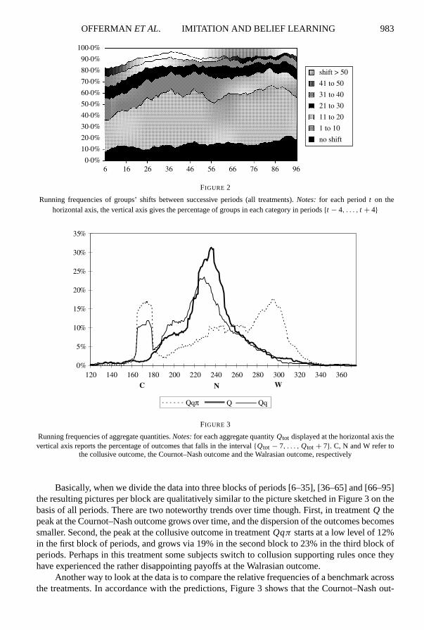
Figure 1 does not display much of a time trend in the overall averages. This raises the ques-tion whether there is any dynamics in the underlying group data at all. To address this questionwe examine for each group of three firms by how much the aggregate quantity changes fromone period to the next. Figure 2 displays the “running frequencies” of groups’ shifts in quantitiesbetween successive periods. The picture is roughly the same for each of the treatments so wepresent them in combination. The production levels change more in the early rounds than in thefinal rounds. For example, about 60% of the groups experience a shift in production by at least11 units from one period to the next in the early periods of the experiment. By period 90 this isreduced to about 35% of the groups. Moreover, despite the fact that production averages acrossgroups remain more or less constant, there appears to exist substantial adjustments in the pro-duction levels of the individual groups, justifying a deeper analysis of the underlying dynamics.

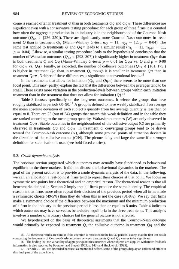
From Figure 1, it appears that although differences in average production levels betweenthe treatments are in the expected direction, they are rather small. Focusing the attention onthe averages is not particularly informative in this experiment however, because it masks someinteresting patterns in the data. Figure 3 shows the “running frequencies” of the aggregateproduction of the three treatments when the data are pooled over all periods. In treatmentQthe production-level is concentrated around the Cournot–Nash outcome of 243 units. IntreatmentQq the distribution of the production-levels is bimodal: as expected, there is a topat the collusive outcome of 168 units. However, the mode of the distribution is at the Cournot–Nash outcome. Again, the distribution of production-levels is bimodal in treatmentQqπ . Ashypothesized, the mode of the distribution is found at the Walrasian outcome of 300 units. Thedistribution also has a top at the collusive outcome. Despite the fact that the average quantityproduced is in the neighbourhood of the Cournot–Nash quantity in this treatment, there is nomode at the Cournot–Nash equilibrium!


100·0%

90·0%

80·0%

70·0%

60·0%

50·0%

40·0%

30·0%

20·0%

10·0%

0·0%6 16 26 36 46 56 66 76 86 96

shift > 50

41 to 50

31 to 40

21 to 30

11 to 20

1 to 10

no shift

FIGURE 2

Running frequencies of groups’ shifts between successive periods (all treatments).Notes: for each periodt on thehorizontal axis, the vertical axis gives the percentage of groups in each category in periods{t − 4, . . . , t + 4}

0%

5%

10%

15%

20%

25%

30%

35%

NC W

Qqπ Q Qq

120 140 160 180 200 220 240 260 280 300 320 340 360

FIGURE 3

Running frequencies of aggregate quantities.Notes:for each aggregate quantityQtot displayed at the horizontal axis thevertical axis reports the percentage of outcomes that falls in the interval{Qtot − 7, . . . , Qtot + 7}. C, N and W refer to

the collusive outcome, the Cournot–Nash outcome and the Walrasian outcome, respectively

Basically, when we divide the data into three blocks of periods [6–35], [36–65] and [66–95]the resulting pictures per block are qualitatively similar to the picture sketched in Figure 3 on thebasis of all periods. There are two noteworthy trends over time though. First, in treatmentQ thepeak at the Cournot–Nash outcome grows over time, and the dispersion of the outcomes becomessmaller. Second, the peak at the collusive outcome in treatmentQqπ starts at a low level of 12%in the first block of periods, and grows via 19% in the second block to 23% in the third block ofperiods. Perhaps in this treatment some subjects switch to collusion supporting rules once theyhave experienced the rather disappointing payoffs at the Walrasian outcome.

Another way to look at the data is to compare the relative frequencies of a benchmark acrossthe treatments. In accordance with the predictions, Figure 3 shows that the Cournot–Nash out-


come is reached often in treatmentQ than in both treatmentsQq andQqπ . These differences aresignificant even with a conservative testing procedure: for each group of three firms it is countedhow often the aggregate production in an industry is in the neighbourhood of the Cournot–Nashoutcome (Qtot ∈ [236, 250]). There are significantly more Cournot–Nash outcomes in treat-ment Q than in treatmentQq (Mann–WhitneyU -test:nQ = 11, nQq = 12, p = 0·04). Thesame test applied to treatmentsQ and Qqπ leads to a similar result (nQ = 11, nQqπ = 11,p = 0·04). Likewise, a similar testing procedure leads to the hypothesized conclusion that thenumber of Walrasian outcomes (Qtot ∈ [293, 307]) is significantly higher in treatmentQqπ thanin both treatmentsQ andQq (Mann–WhitneyU -tests:p = 0·01 for Qqπ vs. Q and p = 0·00for Qqπ vs. Qq). Finally, as expected, the number of collusive outcomes (Qtot ∈ [161, 175])is higher in treatmentQq than in treatmentQ, though it is smaller in treatmentQq than intreatmentQqπ . Neither of these differences is significant at conventional levels.15

In the treatments that allow for imitation (Qq andQqπ) there seems to be more than onefocal point. This may (partly) explain the fact that the differences between the averages tend to besmall. There exists more variation in the production-levels between groups within each imitationtreatment than in the treatment that does not allow for imitation (Q).16

Table 3 focuses specifically on the long-term outcomes. It selects the groups that haveroughly stabilized in periods 60–90.17 A group is defined to have weakly stabilized if on averagethe mean absolute deviation of each subject’s quantity from her average quantity is less than orequal to 8. There are 23 (out of 34) groups that match this weak definition and in the table theyare ranked according to the mean group quantity. Walrasian outcomes (W) are only observed intreatmentQqπ . Stable outcomes in the neighbourhood of the collusive output (C) are primarilyobserved in treatmentsQq and Qqπ . In treatmentQ converging groups tend to be drawntoward the Cournot–Nash outcome (N), although some groups’ points of attraction deviate inthe direction of the collusive output (C/N). The picture is by and large the same if a strongerdefinition for stabilization is used (see bold-faced entries).

5.2. Crude dynamic analysis

The previous section suggested which outcomes may actually have functioned as behaviouralequilibria in the three markets. It did not discuss the behavioural dynamics in the markets. Thegoal of the present section is to provide a crude dynamic analysis of the data. In the following,we call an allocation a rest-point if firms tend to repeat their choices at that point. We focus onsymmetric rest-points for a theoretical and an empirical reason. The theoretical reason is that allbenchmarks defined in Section 2 imply that all firms produce the same quantity. The empiricalreason is that firms more often repeat their decision of the previous period when all firms madea symmetric choice (49·5%) than they do when this is not the case (31·8%). We say that firmsmake a symmetric choice if the difference between the maximum and the minimum productionof a firm in the industry in the previous period is less than or equal to 8 units. Table 4 indicateswhich outcomes may have served as behavioural equilibria in the three treatments. This analysisinvolves a number of arbitrary choices but the general picture is not affected.

We hypothesized on the basis of theoretical arguments that the Cournot–Nash outcomewould primarily be expected in treatmentQ, the collusive outcome in treatmentQq and the

15. All these test results are similar if the attention is restricted to the last 30 periods, except that the first test resultcomparing the frequency of Cournot–Nash outcomes between treatmentsQ andQq ceases to be significant.

16. The finding that the variability of aggregate quantities increases when subjects are supplied with more feedbackinformation is also reported by Fouraker and Siegel (1963, p. 143) and Hucket al. (1999).

17. Periods 91–100 are discarded because, as mentioned before, some of the groups display an end round effect inthis final part of the experiment.


TABLE 3

Long-term outcomes

% Groups converging TreatmentQ TreatmentQ TreatmentQqπ

Weakly 63·6% 66·7% 72·7%Strongly 45·5% 25·0% 36·4%

Mean Mean MeanGroup No. production Outcome production Outcome production Outcome

8 171·3 C29 175·2 C1 177·8 C/N

21 190·3 C/N32 213·9 C/N30 216·4 C/N9 219·0 C/N

15 224·1 C/N24 224·8 C/N19 227·6 C/N31 230·0 C/N22 232·3 C/N25 235·8 N16 239·6 N13 239·7 N18 240·1 N28 243·9 N11 248·5 N27 254·4 N/W7 277·0 N/W

10 279·7 N/W4 293·0 W5 303·3 W

Notes:a group is defined to weakly (strongly) converge if in periods 61–90 the mean absolute deviation of asubject’s production to her average production level averaged over the group is smaller than or equal to 8 (4). Incase of weak convergence, the group’s average production level in periods 61–90 is displayed, and the outcomeis labelled as C(ollusion), N(ash) or W(alras) if it is within 7 units from the collusive (168), Cournot–Nash (243),or Walras (300) outcome, respectively. The entries of strongly converging groups are bold. Outcomes betweencollusion and Cournot–Nash are labelled C/N, and outcomes between Cournot–Nash and Walras as N/W. The leftcolumn displays the group identification number. Groups are ordered on the mean production of their convergencepoint.

TABLE 4

Symmetric rest points

Previous own choicein category TreatmentQ TreatmentQq TreatmentQqπ

40–48 15 16 349–57 (C) 12 354(79%) 485(85%)58–66 161(27%) 166(51%) 136(43%)67–75 239(41%) 332(34%) 121(31%)76–84 (N) 361(55%) 282(27%) 138(60%)85–93 16 28(7%) 140(26%)94–102 (W) 0 9 326(37%)

103–111 0 1 33(18%)112–125 0 9 1

Notes:the first number in a cell displays the number of symmetric outcomes,that is, outcomes in which the difference between the maximum and theminimum production in an industry is smaller than or equal to 8. For morethan 25 symmetric choice situations the second number between parenthesesdisplays the percentage of choices that are exactly the same as the choice inthe previous period.


TABLE 5

Adaptation process of middle firms

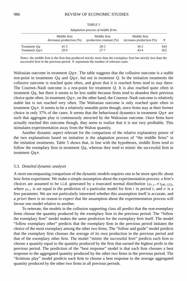
Middle firm Middle firm Middle firmdecreases production (%) production constant (%) increases production (%)N

TreatmentQq 41·5 28·3 30·2 643TreatmentQqπ 29·0 27·7 43·4 452

Notes:the middle firm is the firm that produced strictly more than the exemplary firm but strictly less than thesuccessful firm in the previous period.N represents the number of relevant cases.

Walrasian outcome in treatmentQqπ . The table suggests that the collusive outcome is a stablerest-point in treatmentsQq and Qqπ , but not in treatmentQ. In the imitation treatments thecollusive outcome is reached quite often, and given that it is reached firms tend to stay there.The Cournot–Nash outcome is a rest-point for treatmentQ. It is also reached quite often intreatmentQq, but there it seems to be less stable because firms tend to abandon their previouschoice quite often. In treatmentQqπ , on the other hand, the Cournot–Nash outcome is relativelystable but is not reached very often. The Walrasian outcome is only reached quite often intreatmentQqπ . It seems to be a relatively unstable point though, since firms stay at their formerchoice in only 37% of the cases. It seems that the behavioural dynamics in treatmentQqπ aresuch that aggregate play is continuously attracted by the Walrasian outcome. Once firms haveactually reached this outcome though, they seem to realize that it is not very profitable. Thisstimulates experimentation away from the Walras quantity.

Another dynamic aspect relevant for the comparison of the relative explanatory power ofthe two explanations based on imitation is the adaptation process of “the middle firms” inthe imitation treatments. Table 5 shows that, in line with the hypotheses, middle firms tend tofollow the exemplary firm in treatmentQq, whereas they tend to mimic the successful firm intreatmentQqπ .

5.3. Detailed dynamic analysis

A more encompassing comparison of the dynamic models requires one to be more specific abouthow firms experiment. We make a simple assumption about the experimentation process: a firm’schoices are assumed to be i.i.d. generated by a truncated normal distribution(µi,t , σ )[40,125],whereµi,t is set equal to the prediction of a particular model for firmi in periodt , andσ is afree parameter. We are not particularly interested whether this assumption itself is accurate, anda priori there is no reason to expect that the assumption about the experimentation process willfavour one model relative to another.

To reiterate, the models in the collusion supporting class all predict that the non-exemplaryfirms choose the quantity produced by the exemplary firm in the previous period. The “followthe exemplary firm” model makes the same prediction for the exemplary firm itself. The model“follow exemplary other” predicts that the exemplary firm in the previous period imitates thechoice of the most exemplary among the other two firms. The “follow and guide” model predictsthat the exemplary firm chooses the average of its own production in the previous period andthat of the exemplary other firm. The model “mimic the successful firm” predicts each firm tochoose a quantity equal to the quantity produced by the firm that earned the highest profit in theprevious period. The prediction of the “best response” model is that each firm chooses a bestresponse to the aggregated quantity produced by the other two firms in the previous period. The“fictitious play” model predicts each firm to choose a best response to the average aggregatedquantity produced by the other two firms in all previous periods.


The preceding models all assume that subjects learn in one way or another. However,whether subjects learn or not is something to be decided by the data. Therefore, we also includethree benchmark models: the “collusion plus noise” predicts that a firm always chooses 56, the“Cournot–Nash plus noise” model predicts constant choices of 81 and the “Walras plus noise”model predicts constant choices of 100.

Finally, we compare the results with a model that sets a lower bound on the expectedperformance: the “random model”. This model predicts that each of the 86 possible choices(integers from 40 to 125) is chosen with probability 1/86. Note that the random model is nestedin each of the other models: ifσ → ∞ in one of the models, the random model is obtained.

Table 6 reports the maximum likelihood results for the models described above. Within theclass of collusion supporting models, the learning model follow and guide outperforms both theother learning models and the collusion plus noise benchmark: in both treatmentsQq andQqπ

the follow and guide model yields the better likelihood and the lower estimate forσ . By choosinga production level above their own previous level but below the level of the exemplary other firm,an exemplary firm provides a signal that it wants to move toward the collusive outcome but onlyif at least one other firm also moves in that direction.18 Within the class of Walras supportingmodels, the mimic successful firm model organizes the data much better than the Walras plusnoise model, both in treatmentsQq andQqπ . In the class of Cournot–Nash supporting models,the fictitious play model is better than the best response model in all treatments. However, thestatic Cournot–Nash plus noise model outperforms both learning models. This suggests thatsubjects do not update their beliefs as supposed by either best response or fictitious play models.

As a result, the remainder will focus on the follow and guide model, the mimic successfulfirm model and the Cournot–Nash plus noise model as the candidates of the collusion supporting,the Walras supporting and the Cournot–Nash supporting models, respectively. Each of thesemodels fits the data significantly better than the random model in all treatments (likelihood ratiotest at 1% level).

Remember that in treatmentQ it is impossible to imitate because firms lack the necessaryinformation to do so. Nevertheless, the two imitation models are also estimated for this treatmentto obtain a lower bound on the expected performance of the Cournot Nash plus noise model. Ifone of the imitation models would provide a better fit of the data than the Cournot–Nash plusnoise model in treatmentQ, then we could conclude that the Cournot–Nash plus noise modeldoes a very bad job because it is outperformed by a model that cannot be true. However, wefind that the Cournot–Nash plus noise model beats the imitation models both on the criterionof likelihood and on the criterion of the estimateσ . In treatmentsQq and Qqπ firms had inprinciple sufficient information to behave in accordance with each of the models. The followand guide model outperforms the mimic successful firm model in treatmentQq both on thelikelihood and the estimate ofσ . The ordering is reversed in treatmentQqπ . There, the mimicsuccessful firm model outperforms the follow and guide model on the basis of the likelihood,though the follow and guide model yields a somewhat lower estimate forσ .

These results are by and large in line with the predictions described in Table 2. The maindifference is that belief learning does not seem to be the reason for observing the Cournot–Nashoutcome in treatmentQ. A static Cournot–Nash model organizes the data better than either ofthe belief learning models.

Table 4 suggested that the imitation treatmentsQq and Qqπ contain more than one rest-point each. This may reflect heterogeneity in the population. Perhaps one part of the population

18. Note that the follow and guide rule prescribes the exemplary firm to provide a mild punishment only. We alsolooked at models that involve a stronger punishment by the exemplary firm. For instance, one such rule prescribes theexemplary firm to choose the average production level of the other firms in the previous period. Such rules perform worsethan the follow and guide rule. Exemplary firms appear to employ relatively mild punishments indeed.


TABLE 6

Maximum likelihood estimates simple models

TreatmentQ TreatmentQq TreatmentQqπ

n = 3267 n = 3564 n = 3267

Collusion supportingmodelsCollusion plus noise − log L = 14,232·3 − log L = 15,382·6 − log L = 14,513·9

σ = 36·40(0·81) σ = 32·49(0·61) σ = 66·40(3·90)

Follow the exemplary − log L = 13,949·3 − log L = 15,078·5 − log L = 13,927·2firm σ = 23·87(0·44) σ = 23·27(0·39) σ = 23·78(0·43)

Follow and guide − log L = 13,936·4 − log L = 15,052·1 − log L = 13,901·7σ = 23·12(0·42) σ = 22·47(0·37) σ = 23·12(0·41)

Follow exemplary − log L = 13,987·4 − log L = 15,170·0 − log L = 13,949·9other firm σ = 23·85(0·45) σ = 23·48(0·40) σ = 24·16(0·44)

Walras supportingmodelsWalras plus noise − log L = 14,501·4 − log L = 15,875·4 − log L = 14,469·5

σ = 51·95(2·67) σ = 653·24(850·57) σ = 45·65(1·87)

Mimic successful firm − log L = 14,118·6 − log L = 15,461·7 − log L = 13,842·2σ = 26·10(0·54) σ = 28·42(0·59) σ = 23·81(0·42)

Cournot–Nashsupporting modelsCournot–Nash plus − log L = 13,736·5 − log L = 15,326·8 − log L = 14,271·2noise σ = 17·16(0·26) σ = 20·27(0·35) σ = 24·24(0·55)

Best response − log L = 14,084·5 − log L = 15,772·1 − log L = 14,548·9σ = 21·37(0·40) σ = 34·98(1·29) σ = 86·58(16·35)

Fictitious play − log L = 13,837·6 − log L = 15,687·2 − log L = 14,516·2σ = 18·09(0·29) σ = 28·60(0·79) σ = 45·11(2·73)

Random − log L = 14,552·4 − log L = 15,875·3 − log L = 14,552·4

Notes:the likelihood is computed on the basis of all choices from period 2–100 of all subjects in a treatment. Themodels are explained in the main text. The standard error of an estimated parameter is displayed between parentheses.

uses one dynamic rule while another part uses another. To investigate this possibility, moregeneral models are formulated. The most general model considered here allows a firm to useany of the three models. In the following, letPf g denote the probability that an arbitrary firmuses the follow and guide model;Pms f and Pnsh denote the probability that a firm uses themimic successful firm model and the Cournot–Nash plus noise model respectively. We definePf g + Pms f + Pnsh = 1. Let qi,t denote the quantity produced by firmi in periodt . Then, theunconditional likelihood function of firmi ’s choices from period 2–100L(qi,2, . . . , qi,100) isgiven by

L(qi,2, . . . , qi,100) = Pf g ∗

∏100

t=2L(qi,t | f g) + Pms f ∗

∏100

t=2L(qi,t | ms f)

+ Pnsh ∗

∏100

t=2L(qi,t | nsh),

whereL(qi,t | f g), L(qi,t | ms f) andL(qi,t | nsh) denote the conditional probability that firmichooses quantityqi,t at periodt when it follows and guides, when it mimics the successful firm,and when it chooses the Cournot–Nash production level in a noisy way, respectively.

The likelihood functions for three general models that allow for two dynamic rules each areobtained by setting eitherPf g, Pms f or Pnsh equal to 0 in the equation describing the likelihood


TABLE 7

Maximum likelihood estimates general models imitation treatments

TreatmentQq TreatmentQqπ

n = 3564 n = 3267

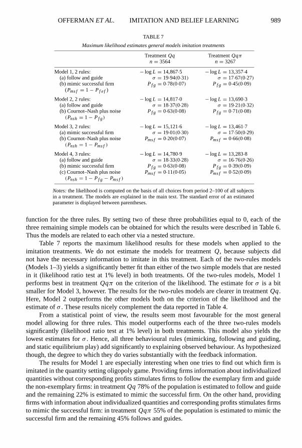
Model 1, 2 rules: − log L = 14,867·5 − log L = 13,357·4(a) follow and guide σ = 19·94(0·31) σ = 17·67(0·27)(b) mimic successful firm Pf g = 0·78(0·07) Pf g = 0·45(0·09)

(Pms f = 1 − Pf e f )

Model 2, 2 rules: − log L = 14,817·0 − log L = 13,690·3(a) follow and guide σ = 18·37(0·28) σ = 19·21(0·32)(b) Cournot–Nash plus noise Pf g = 0·63(0·08) Pf g = 0·71(0·08)

(Pnsh = 1 − Pf g)

Model 3, 2 rules: − log L = 15,121·6 − log L = 13,461·7(a) mimic successful firm σ = 19·01(0·30) σ = 17·50(0·29)(b) Cournot–Nash plus noise Pms f = 0·20(0·07) Pms f = 0·66(0·08)

(Pnsh = 1 − Pms f)

Model 4, 3 rules: − log L = 14,780·9 − log L = 13,283·8(a) follow and guide σ = 18·33(0·28) σ = 16·76(0·26)(b) mimic successful firm Pf g = 0·63(0·08) Pf g = 0·39(0·09)(c) Cournot–Nash plus noise Pms f = 0·11(0·05) Pms f = 0·52(0·09)

(Pnsh = 1 − Pf g − Pms f)

Notes:the likelihood is computed on the basis of all choices from period 2–100 of all subjectsin a treatment. The models are explained in the main text. The standard error of an estimatedparameter is displayed between parentheses.

function for the three rules. By setting two of these three probabilities equal to 0, each of thethree remaining simple models can be obtained for which the results were described in Table 6.Thus the models are related to each other via a nested structure.

Table 7 reports the maximum likelihood results for these models when applied to theimitation treatments. We do not estimate the models for treatmentQ, because subjects didnot have the necessary information to imitate in this treatment. Each of the two-rules models(Models 1–3) yields a significantly better fit than either of the two simple models that are nestedin it (likelihood ratio test at 1% level) in both treatments. Of the two-rules models, Model 1performs best in treatmentQqπ on the criterion of the likelihood. The estimate forσ is a bitsmaller for Model 3, however. The results for the two-rules models are clearer in treatmentQq.Here, Model 2 outperforms the other models both on the criterion of the likelihood and theestimate ofσ . These results nicely complement the data reported in Table 4.

From a statistical point of view, the results seem most favourable for the most generalmodel allowing for three rules. This model outperforms each of the three two-rules modelssignificantly (likelihood ratio test at 1% level) in both treatments. This model also yields thelowest estimates forσ . Hence, all three behavioural rules (mimicking, following and guiding,and static equilibrium play) add significantly to explaining observed behaviour. As hypothesizedthough, the degree to which they do varies substantially with the feedback information.

The results for Model 1 are especially interesting when one tries to find out which firm isimitated in the quantity setting oligopoly game. Providing firms information about individualizedquantities without corresponding profits stimulates firms to follow the exemplary firm and guidethe non-exemplary firms: in treatmentQq 78% of the population is estimated to follow and guideand the remaining 22% is estimated to mimic the successful firm. On the other hand, providingfirms with information about individualized quantities and corresponding profits stimulates firmsto mimic the successful firm: in treatmentQqπ 55% of the population is estimated to mimic thesuccessful firm and the remaining 45% follows and guides.


We do not wish to attach too much weight to the exact numbers in these estimation resultsthough. Apart from the fact that the number of subjects is limited and that we only study oneparticular market structure, we have restricted our attention to a (plausible) subset of the potentiallearning rules with clear long-term predictions. Nevertheless, the estimated differences betweenthe treatments are substantial and they clearly indicate that feedback information affects thebehavioural rules that are adopted by the subjects.

6. CONCLUSION

In this paper we test whether different feedback information triggers different behavioural ruleswhich in turn lead to different outcomes in a quantity setting oligopoly experiment. With onlyfeedback information about the aggregate quantities produced (treatmentQ), the frequencydistribution is unimodal and more or less symmetric around the Cournot–Nash equilibrium.When feedback information about individual quantities is available (treatmentQq), there aretwo peaks: one at the Cournot–Nash equilibrium, and one at the collusive outcome. When inaddition information on the corresponding individualized profits is provided (treatmentQqπ ),the frequency distribution is also bi-modal, with peaks around the collusive and the competitiveoutcome. In the latter case, Cournot–Nash seems to have lost all of its attraction.

A qualitative look at the underlying dynamics permits us to sharpen these results. TheCournot–Nash outcome is the only candidate behavioural rest point in treatmentQ. In treatmentsQq andQqπ , however, it turns out that the main candidate to serve as a behavioural rest pointis the collusive outcome. Although the Cournot–Nash and the competitive outcome are reachedquite often in treatmentsQq and Qqπ , respectively, they are abandoned at a much higher ratethan the collusive outcome. A maximum likelihood procedure corroborates the hypothesizedrelationship between information treatment and dynamic rule of conduct to a large extent. Thebest fit is given by “following the exemplary firm and guiding the non-exemplary firms” intreatmentQq, and by “mimicking the successful firm” in treatmentQqπ . In treatmentQ,however, belief learning models are outperformed by static equilibrium play (plus noise).

Mimicking the successful firm could be thought of as a low cognitive effort rule in thisgame. Following the exemplary firm and guiding non-exemplary firms is a higher cognitiveeffort algorithm. To follow requires finding out the exemplary firm, which is never part of theimmediately available information. And to guide involves at least some basic strategic reasoning.Belief learning and equilibrium play seem to provide the highest cognitive challenge. Theserequire a firm to compute or estimate the best response function, which is not so easy for thepresent game. As information conditions deteriorate from treatmentsQqπ , to Qq, to Q, subjects’behaviour tends to become more sophisticated, from mimicking, to following, to equilibriumplay. It is as if subjects try to offset the deterioration of information by more sophisticatedbehaviour. Perhaps the presence of easy-to-use (but suboptimal) clues like information aboutrivals’ profits discourages people to think deeply about the decision problem.

The success of the collusive outcome especially in treatmentQq but also in treatmentQqπ

may, at least partly, be due to the repeated nature of the game. It seems likely that some ofthe players who follow the exemplary firm and guide the non-exemplary firms are motivatedto do so by the fact that the game is repeated. They may hope that following catches on,leading to a movement towards the collusive outcome. In future work it would be interestingto examine the extent to which following depends on the repeated nature of the game. This couldbe done by running an experiment in which players are rematched with different rivals after eachperiod. Possibly, this would increase the success of the other theoretical benchmarks, Walras andCournot–Nash.


A complementary approach is adopted in Hucket al. (1999). Apart from many smallerdifferences in the details of the design and procedure (e.g.number of firms, number of rounds,cost and demand functions, the use of profit calculators), there are two major differences betweentheir and our approach. First, contrary to Hucket al. (and also Fouraker and Siegel (1963)),we provide subjects with full information about demand and cost functions in all treatments.Hence, in principle our subjects always have enough information to calculate any benchmarkthat they like. Second, we employ a treatment (Qq) which provides feedback information inbetween complete feedback of individual quantities and profits and no individualized feedback.This, we believe, gives a sharp view on the relative importance of mimicking the successful firmand following (the latter of which is not considered in Hucket al.). Huck et al. show that themarket outcome becomes more competitive when information about demand and cost conditionsdeteriorates. Thus, an intriguing pattern emerges: when information about the realized profits ofcompetitors deteriorates (like going from our treatmentQqπ to treatmentQq), the competitiveoutcome is observed less frequently and when information about market conditions deteriorates(as studied in Hucket al.) the opposite effect is observed. This pattern can be explained in termsof the decision costs and availability of alternative behavioural rules. On the one hand, wheninformation about competitors’ profits deteriorates, mimicking the successful firm becomes morecostly relative to some other rules, like following the exemplary firm and guiding non-exemplaryfirms. This discourages mimicking of the successful firm, diminishing the force towards thecompetitive outcome. On the other hand, when information about market conditions deteriorates,it is more costly or even impossible to implement cognitively more expensive rules like belieflearning and following. This increases the relative attractiveness of imitating the successful firm,thus increasing the force towards competitive outcomes.

Finally, it is useful to recall that Vega-Redondo’s motivation for a model of imitation ofthe successful firm is not based on bounded rationality concerns as much as on evolutionaryconsiderations. According to the evolutionary approach it is relative rather than absoluteperformance that matters for success. It may then be a sensible strategy for a firm to increaseits quantity, even if total production is at or above the Cournot–Nash equilibrium. By doing so,a firm will hurt itself, but it will hurt the other firms even more. Consistent with this suggestion,within each group of three firms the one producing the highest average quantity is generally theone earning the highest profit. However, this advantage is more than offset by the fact that groupsof followers perform better than groups of mimics. In our experiment, the Pearson correlationcoefficient between firms’ average production and their average profit is significantly negative(r = −0·65, p = 0·001,n = 102). If the relative performance of firms is determined acrossindustries and not merely within industries, then following the exemplary firm and guidingnon-exemplary firms is a more successful rule of conduct than mimicking the successful firm.As already argued in the evolutionary theory of cultural transmission by Boyd and Richerson(1991, 1993), intergroup rivalry may serve as a potential explanation for a tendency to imitatecooperative behaviour. From this perspective it is not so straightforward what would be the mostsuccessful strategy of imitation: mimic the villain or follow the saint?

APPENDIX A. SKETCHES OF THE PROOFS OF THE RESULTS IN SECTION 2

Result1 (for details see Vega-Redondo(1997))

First note that only symmetric states(q1 = q2 = q3) can be limit states of the imitation dynamics. One round of imitationwill bring about a symmetric state from any state with asymmetric quantity choices. When players arrive at a symmetricstate, it is obvious that imitation will keep them there. Hence, any symmetric outcome could potentially be a limit stateof the imitation process alone. The imitation dynamics, however, “resolve” this indeterminacy of the imitation dynamics.


The centrepiece of the proof is that for eachq 6= qW and 1≤ k ≤ n (n = 3 in our experiment), the followinginequality holds:

P((n − k)q + kqW)qW− C(qW) > P((n − k)q + kqW)q − C(q). (A.1)

To see this, first note that

[P(nqW) − P((n − k)q + kqW)]q > [P(nqW) − P((n − k)q + kqW)]qW. (A.2)

This follows from the fact thatP is decreasing, so that the price difference in the inequality is negative whenq < qW

and positive whenq > qW. In either case the inequality holds. Now rewrite (A.2) as follows:

P(nqW)q + P((n − k)q + kqW)qW > P(nqW)qW+ P((n − k)q + kqW)q. (A.3)

SubtractingC(q) + C(qW) from either side and rearranging, we obtain

[P((n−k)q +kqW)qW−C(qW)]− [P((n−k)q +kqW)q −C(q)] > [P(nqW)qW

−C(qW)]− [P(nqW)q −C(q)].(A.4)

From the definition ofqW, the Walrasian equilibrium, it follows that the R.H.S. of inequality (A.4) is no smaller thanzero. This ensures that the L.H.S. of (A.4) is larger than zero, which is equivalent to (A.1).

Insertingk = 1 in inequality (A.1) tells us that if one firm producesqW and the other firms produce some otherquantityq, then the firm producingqW will earn the highest profit. Hence, from any symmetric state in which the firmsproduce some quantityq 6= qW, it will take only one suitable mutation (plus one round of imitation) to move the state tothe Walrasian outcome.

Insertingk = n − 1 in inequality (A.1) tells us that if all firms except one produce the Walrasian quantity, thenthe firms producingqW will earn a higher profit than the firm producing some other quantityq. Hence, one round ofimitation will bring the latter firm back to the Walrasian quantity. In other words, starting from the Walrasian outcome,one mutation will not be enough to move the process away from this outcome. At least, two mutations are necessary toescape the Walrasian outcome.

We have seen that (a) arriving at a symmetric outcome involves only imitation and no mutation, (b) arriving atqW from any other symmetric outcome involves only one (suitable) mutation, and (c) escaping the Walrasian outcomerequires at least two mutations. With the help of the graph-theoretic techniques of Freidlin and Wentzel (1984), thesefacts can be used to show that withε → 0, the Walrasian outcome is the unique stochastically stable state.

Result 2

For the dynamics induced by each of the following rules only symmetric states can be limit states. Starting from any state,after one round (under “follow the exemplary firm”) or two rounds (under “follow and guide” or “follow the exemplaryother firm”) the following dynamics will bring about a symmetric state. At the same time the probability of leaving asymmetric state with following alone is zero. The introduction of a small probability (ε) of mutation singles out (whenε → 0) the unique stochastically stable state, namely the collusive outcome in which all firms produceqC (= 56 in ourexperiment).

The arguments on which this claim rests are similar to the ones for Result 1, but easier to establish. The rules“follow the exemplary firm”, “follow and guide” and “follow the exemplary other firm” all assume that the non-exemplaryfirms follow the exemplary firm. Hence, if at least one firm producesqC , then—no matter what the other firms produce—the firm (or one of the firms) producingqC will be the exemplary firm. One round of following will then ensure that atleast two firms produce at the collusive output. In the next round they will be exemplary for each other and remain atthe collusive outcome, and—should it have moved away—the third firm will return to the collusive output. Hence, onlyone suitable mutation is needed to arrive at the collusive state. Second, starting from the collusive outcome, suppose onefirm mutates and produces some other quantityq 6= qC . Then the firms still producingqC are the exemplary firms, andthe mutant will return to the collusive output. Hence, at least two mutations are needed to escape the collusive outcome.These features ensure that the collusive outcome is the unique stochastically stable state of the following plus mutationdynamics asε → 0.

Result 319

Best response dynamics and fictitious play are special cases of the adaptive learning models analysed in Milgrom andRoberts (1991). Roughly speaking, a learning process is consistent with adaptive learning if each player eventually

19. The proof was suggested by one of the referees.


chooses strategies that are a best response to some beliefs over competitors’ strategies, where near zero probability isassigned to strategies that have not been played for a sufficiently long time. Milgrom and Roberts show that a processthat is consistent with adaptive learning converges to the serially undominated set, that is, the set of strategies that surviveiterated elimination of strongly dominated strategies.

The serially undominated set of the oligopoly game in Section 2 is the Cournot–Nash equilibrium. This followsfrom the fact that the best-reply mapping of the game is a contraction. A sufficient condition for a contraction (see,e.g.Vives (1999)) is

∂2πi

(∂qi )2

+

∑i 6= j

∣∣∣∣∣ ∂2πi

∂qi ∂q j

∣∣∣∣∣ < 0.

Since∂2πi /(∂qi )2

= P′′qi + 2P′− C′′, and6i 6= j |(∂

2πi )/(∂qi ∂q j )| = −2P′′qi − 2P′ this condition requires that−P′′qi − C′′ < 0, which follows immediately fromP′′ > 0 andC′′ > 0.

This result cannot be directly applied though, since the subjects in our experiment choose from the finite strategyset {40, 41, . . . , 125}. It turns out, however, that also on the finite grid the Nash equilibrium is the unique seriallyundominated strategy profile. The best response toQ−i = 80 is qi = 102 and the best response toQ−i = 250 isqi = 60. Given that the profit function is strictly concave and that 80≤ Q−i ≤ 250, the first round of elimination ofdominated strategies leaves us with the quantity choices 60≤ qi ≤ 102. In the second round we can use the restriction120 ≤ Q−i ≤ 204 to leave us with the undominated quantity choices 70≤ qi ≤ 92. Repeating this process leaves uswith qi = 81 after eight steps of elimination.20

Just as in the imitation models we can add noise (experimentation) to the learning process by assuming that ineach round with probabilityε a player randomly chooses some quantity from the feasible set according to a probabilitydistribution with full support. Theorem 4 in Young (1993) can then be used to establish that the Cournot–Nash outcomeis the unique stochastically stable state of the perturbed belief learning process.

APPENDIX B

This appendix presents the instructions and prints of the computer screens that were used in each of the three treatments.The figures and tables that were used to communicate the market structure will be sent on request. After a short welcome,subjects read the computerized instructions at their own pace. They could go forward and backward in the program. At thestart of the instructions it was explained how they should use the computer. A translated version of the Dutch instructionsruns as follows:

Experiment

You will make decisions for a firm in this experiment. You will be asked repeatedly to determine the quantity that yourfirm will produce. Your payoff will depend on your production and the production of two other firms. The decisions forthese two other firms will be made by two other participants of the experiment. For convenience we will refer to theseother firms as firms A and B.

You will be matched with the same two other firms throughout the experiment. The same participants will makethe decisions for these two firms. You will not know with whom you will be matched, like others will not know withwhom they will be matched. Anonymity is ensured.

Own production and costs(table)

The experiment will last for 100 periods. Each period you will decide how much your firm produces. Your productionmust be greater than or equal to 40 units and smaller than or equal to 125 units. You may only choose integer numbers.For example, it is not allowed to produce half units.

Producing involves costs. There is a cost-form on your table. On one side of this form the cost-table is displayed.Each time you pick a lower row of the table, your production increases by 10 units. Each time you pick a column moreto the right of the table, your production increases by 1 unit. For example, if you want to know the costs of producing 79units, you descend in the left column until you have reached the row where 70 units are produced. Then you shift ninecolumns to the right to find the cell containing the costs of a production-quantity of 79 units. A production of 79 unitscosts 702 points.

20. A complication, however, is that in the experiment payoffs are rounded to two decimals (cents), as aconsequence of which the payoff function is not strictly concave. It turns out that this halts the elimination processafter Step 7, at which point the surviving set of strategies still consists ofqi ∈ {80, 81, 82}. Hence, for practical purposesthis is the serially undominated set to which adaptive learning processes will converge.


Own production and costs(graph)

The other side of the cost-form displays graphically the relationship between quantity produced and costs. You find thecosts of a certain production-quantity by searching this quantity on the horizontal axis and by determining the level ofthe costs at this quantity on the vertical axis.

Above the graph the formula is displayed which is used to compute the costs. Both the table and the graph areconstructed with the help of this formula. Therefore, the table and the graph convey exactly the same information. Youmay decide for yourself which representation you want to use in the experiment.

Question

What will be your costs if you produce 87 units?[Subjects had to type in the correct answer before they could continue with the instructions. If they did not answercorrectly, the relevant part of the instructions was repeated in different terms before the question was posed again.]

Total production and price(table)

The price that you will receive for each unit produced depends on the total production. The total production is the sumof the production of firm A, the production of firm B and your production. Since firms A and B each will also producebetween 40 and 125 units, total production will not be smaller than 120 units and not be greater than 375 units.

There is a price-form on your table. One side of this form shows the price-table. This table gives the prices foreach possible total production. The table works the same way as the cost-table. Each time you pick a lower row of thetable, total production increases by 10 units. Each time you pick a column more to the right of the table, total productionincreases by 1 unit. For example, if total production consists of 272 units, you descend in the left column until you havereached the row where 270 units are produced. Then you shift two columns to the right to find the cell containing theprice of a total production-quantity of 272 units.

Total production and price(graph)

The other side of the price-form displays graphically the relationship between total quantity produced and price. You findthe price of a certain production-quantity by searching this quantity on the horizontal axis and by determining the levelof the price at this quantity on the vertical axis.

Again, above the graph the formula is displayed which is used to compute the price. Both the table and the graphare constructed with the help of this formula. You may decide for yourself which representation you want to use in theexperiment.

Question

What will be the price if you produce 87 units, firm A produces 66 units and firm B produces 102 units?[Again, subjects had to type in the correct answer before they could continue with the instructions.]

Production and profit

Each period your revenue is equal to your produced quantity multiplied by the price. Your profit is your revenue minusthe costs of your production.

The circumstances of production are exactly the same for firms A and B as they are for you. The costs of theirproduction is determined in a similar way as your production. They receive the same price for each unit they produce asyou receive.

The experiment lasts for 100 periods. Each period the circumstances of production will be the same as describedabove. Your payoff in the experiment is equal to the sum of your profits in each of the 100 periods. These profits aredenoted in points.

At the end of the experiment your points will be exchanged for real money. For each 1300 points you willreceive one guilder.

Then subjects were made familiar with the screens that they would see in the experiment. The instructions wereexactly the same for treatmentQ, treatmentQq and treatmentQqπ , except for the screen where information about the


results of the previous period was communicated. Before the experiment started, a handout was given to the subjectswith a summary of the instructions and the cost and price-tables were projected on the wall.

Period:

Total earnings: 2356.67

4

points.

Production:Your decision:

Type your production quantityand press Enter.

Translation of the computer screenUpper part screen (same for all conditions)

The results of the previous period:

Your production: 76 The price: 19.19Your revenue: 1458.44

Your costs: 662.55Your earnings: 795.89

146

222Total production:Production of others:

Lower part screen: Results window Q


Your: 76 The price: 19.19Total production: 222

Your revenue: 1458.44Your costs: 662.55

Your earnings: 795.89

62

84B:A:

Lower part screen: Results window Qq

Production:


Your: 76 The price: 19.19Total production: 222

Your revenue: 1458.44Your costs: 662.55

62

84

795.89701.59

842.09B:A:

Lower part screen: Results window Qqπ

Production: Earnings:


Acknowledgements. The authors are thankful for comments by participants of the Amsterdam Workshop onExperimental Economics and the meeting of the Economic Science Association, and by Rachel Croson, Charles Holt,Cars Hommes, Georg Kirchsteiger, and Rob Moir, in particular. Very constructive comments were provided by threereferees. The research is made possible by a grant from the Netherlands’ Organization for Scientific Research (to TheoOfferman) and a fellowship from the Royal Netherlands’ Academy of Arts and Sciences (to Jan Potters).

REFERENCESABBINK, K. and SADRIEH, A. (1995), “RatImage—Research Assistance Toolbox for Computer-Aided Human

Behavior Experiments”(Discussion Paper No. B-325, University of Bonn).ABREU, D. and RUBINSTEIN, A. (1988), “The Structure of Nash Equilibrium in Repeated Games with Finite

Automata”,Econometrica, 56, 1259–1281.BANDURA, A. (1986) Social Foundations of Thought and Action. A Social Cognitive Theory(New Jersey: Prentice-

Hall).BOYD, R. and RICHERSON, P. (1991), “Culture and Cooperation”, in R. Hinde and J. Groebel (eds.)Cooperation and

Prosocial Behavior(Cambridge: Cambridge University Press).BOYD, R. and RICHERSON, P. (1993), “Rationality, Imitation and Tradition”, in R. Day and P. Chen (eds.)Nonlinear

Dynamics and Evolutionary Economics(Oxford: Oxford University Press).BOYLAN, R. T. and EL-GAMAL, M. A. (1993), “Fictitious Play: A Statistical Study of Multiple Economic

Experiments”,Games and Economic Behavior, 5, 205–222.BRANDTS, J. and HOLT, C. A. (1992), “An Experimental Test of Equilibrium Dominance in Signaling Games”,

American Economic Review, 82, 1350–1365.CHEUNG, Y. W. and FRIEDMAN, D. (1997), “Individual Learning in Normal Form Games: Some Laboratory Results”,

Games and Economic Behavior, 19, 46–76.CONLISK, J. (1980), “Costly Optimizers versus Cheap Imitators”,Journal of Economic Behavior and Organization, 1,

275–293.CONLISK, J. (1988), “Optimization Cost”,Journal of Economic Behavior and Organization, 9, 213–228.CONLISK, J. (1996), “Why Bounded Rationality?”,Journal of Economic Literature, 34, 669–700.DAUGHETY, A. (1985), “Reconsidering Cournot: The Cournot Equilibrium is Consistent”,Rand Journal of Economics,

16, 368–379.EL-GAMAL, M. A., M CKELVEY, R. D. and PALFREY, T. R. (1994), “Learning in Experimental Games”,Economic

Theory, 4, 901–922.FOURAKER, L. E. and SIEGEL, S. (1963)Bargaining Behavior(New York: McGraw-Hill).FRASER, C. (1994), “Conjectural Variations”, in J. Cable (ed.)Current Issues in Industrial Organizations(Hampshire:

Macmillan).FREIDLIN, M. I. and WENTZEL, A. D. (1984)Random Perturbations of Dynamical Systems(New York: Springer).FUDENBERG, D. and MASKIN, E. (1986), “The Folk Theorem in Repeated Games with Discounting or with

Incomplete Information”,Econometrica, 54, 533–554.HO, T. and WEIGELT, K. (1996), “Task Complexity, Equilibrium Selection, and Learning: An Experimental Study”,

Management Science, 42, 659–679.HOLT, C. A. (1995), “Industrial Organization: A Survey of Laboratory Research”, in J. H. Kagel and A. E. Roth (eds.)

The Handbook of Experimental Economics(Princeton: Princeton University Press) 349–443.HUCK, S., NORMANN, H. T. and OECHSSLER, J. (1999), “Learning in Cournot Oligopoly—An Experiment”,

Economic Journal, 109, C80–C95.KREPS, D. M., MILGROM, P., ROBERTS, J. and WILSON, R. (1982), “Rational Cooperation in the Finitely Repeated

Prisoners’ Dilemma”,Journal of Economic Theory, 27, 245–252.MARTIN, S. (1993)Advanced Industrial Economics(Oxford: Blackwell Publishers).MILGROM, P. and ROBERTS, J. (1982), “Predation, Reputation, and Entry Deterrence”,Journal of Economic Theory,

27, 280–312.MILGROM, P. and ROBERTS, J. (1991), “Adaptive and Sophisticated Learning in Normal Form Games”,Games and

Economic Behavior, 3, 82–100.MOOKHERJEE, D. and SOPHER, B. (1994), “Learning Behavior in an Experimental Matching Pennies Game”,Games

and Economic Behavior, 7, 62–91.OFFERMAN, T., SCHRAM, A. and SONNEMANS, J. (1998), “Quantal Response Models in Step-Level Public Good

Games”,European Journal of Political Economy, 14, 89–100.OFFERMAN, T. and SONNEMANS, J. (1998), “Learning by Experience and Learning by Imitating Successful Others”,

Journal of Economic Behavior and Organization, 34, 559–575.PARTOW, Z. and SCHOTTER, A. (1993), “Does Game Theory Predict Well for the Wrong Reasons?”(Discussion Paper

RR 93-46, New York University).PINGLE, M. (1995), “Imitation versus Rationality: An Experimental Perspective on Decision Making”,Journal of Socio-

Economics, 24, 281–315.PINGLE, M. and DAY, R. (1996), “Modes of Economizing Behavior: Experimental Evidence”,Journal of Economic

Behavior and Organization, 29, 191–209.ROSENTHAL, R. W. (1993), “Rules of Thumb in Games”,Journal of Economic Behavior and Organization, 22, 1–14.ROTH, A. and EREV, I. (1995), “Learning in Extensive Form Games: Experimental Data and Simple Dynamic Models

in the Intermediate Term”,Games and Economic Behavior, 8, 164–212.


SARASON, I. G., SARASON, B. R., PIERCE, G. R. and SHEARIN, E. N. (1991), “A Social Learning Approach toIncreasing Blood Donations”,Journal of Applied Social Psychology, 21, 896–918.

SCHERER, F. and ROSS, D. (1990)Industrial Market Structure and Economic Performance(Boston: Houghton Mifflin).SELL, J. and WILSON, R. (1991), “Levels of Information and Contributions to Public Goods”,Social Forces, 70,

107–124.SELTEN, R., MITZKEWITZ, M. and UHLIG, G. R. (1997), “Duopoly Strategies Programmed by Experienced Players”,

Econometrica, 65, 517–555.SHUBIK, M. (1975), “Oligopoly Theory, Communication and Information”,American Economic Review, 65, 280–283.SINCLAIR, P. (1990), “The Economics of Imitation”,Scottish Journal of Political Economy, 37, 113–144.SLADE, M. (1994), “Empirical Games: the Oligopoly Case”,Canadian Journal of Economics, 26, 368–402.THEOCHARIS, R. D. (1960), “On the Stability of the Cournot Solution on the Oligopoly Problem”,Review of Economic

Studies, 27, 133–134.VAN HUYCK, J. B., BATALLIO, R. C. and BEIL, R. O. (1990), “Tacit Coordination Games, Strategic Uncertainty, and

Coordination Failure”,American Economic Review, 80, 234–248.VEGA-REDONDO, F. (1997), “The Evolution of Walrasian Behavior”,Econometrica, 65, 375–384.VIVES, X. (1999)Oligopoly Pricing: Old Ideas and New Tools(Cambridge, MA and London: MIT Press).YOUNG, H. P. (1993), “The Evolution of Conventions”,Econometrica, 61, 57–84.

Documents

Imitation and Belief Learning in an Oligopoly Experimentpeople.exeter.ac.uk/dgbalken/EE08/Offermann.pdf · imitation, we hypothesize this treatment to be relatively favourable for