Impact assessment of push-pull technology on incomes,

productivity and poverty among smallholder households in

Eastern Uganda

Chepchirchir R, Macharia I , Murage A.W, Midega C.A.O., Khan Z. R

Invited paper presented at the 5th International Conference of the African Association of

Agricultural Economists, September 23-26, 2016, Addis Ababa, Ethiopia

Copyright 2016 by [authors]. All rights reserved. Readers may make verbatim copies of this

document for non-commercial purposes by any means, provided that this copyright notice

appears on all such copies.

1

Impact assessment of push-pull technology on incomes, productivity and poverty among

smallholder households in Eastern Uganda

Chepchirchir R1,2

, Macharia I2 , Murage A.W

3, Midega C.A.O

1.,

Khan Z. R

1

1International Centre of Insect Physiology and Ecology (icipe), P.O. Box, 30772- 00100,

Nairobi, Kenya

2Kenyatta University, Department of Agribusiness Management and Trade, P.O. Box 43844,

00100 Nairobi, Kenya

3Kenya Agricultural and Livestock Research Organization (KALRO), P.O BOX 25-20117,

Naivasha, Kenya

Abstract

The paper evaluates the impact of adoption of push-pull technology (PPT) on household

welfare in terms of productivity, incomes and poverty status measured through per capita

food consumption in eastern Uganda. Cross sectional survey data was collected from 560

households in four districts in the region: Busia, Tororo, Bugiri and Pallisa, in November and

December 2014. Tobit model was used to determine the intensity of adoption of the

technology whereas generalized propensity scores (GPS) was applied to estimate the dose-

response function (DRF) relating intensity of adoption and household welfare. Results

revealed that with increased intensity of PPT adoption, probability of being poor declines

through increased yield, incomes, and per capita food consumption. With an increase in the

area allocated to PPT from 0.025 to 1 acre, average maize yield increases from 27 kgs to

1,400 kgs, average household income increases from 135 USD (UGX 370,000) to 273 USD

(UGX 750,000) and per capita food consumption increases from 15 USD (UGX 40,000) to

27 USD (UGX 75,000). The average probability of being poor declines from 48% to 28%:

This implies that increased investment on PPT dissemination and expansion is essential for

poverty reduction among smallholder farmers.

Key words: Push-pull technology, generalized propensity score, household welfare, Uganda

Introduction

Agricultural productivity is one of the key determinants of agricultural growth (Salami,

2010). Progress towards food and nutritional security requires that food is available,

accessible and of sufficient quantity and quality (Mellor, 1999; FAO, 2012). Although

increase in agricultural productivity is a necessary condition for progress in poverty and

hunger reduction, it is not sufficient especially in the face of rapidly growing human

population. Hence inclusive agricultural growth that promotes equitable access to food, assets

and resources, especially for poor and vulnerable people is key. This is particularly so in the

developing world where majority of the poor and hungry people live in rural areas, and where

family farming and smallholder agriculture is a prevailing mode of farm organization (FAO,

2012; Kosura, 2013). Growth in family farming and smallholder agriculture through labour

2

and land productivity increases has significant positive effects on the livelihoods of the poor

through increases in food availability and incomes (FAO, 2015).

Cereal crops, including maize (Zea mays L.), sorghum (Sorghumbicolor (L.) Moench), and

rice (Oryza sativa L.) are the most important food and cash crops for millions of rural farm

families in sub-Saharan Africa (SSA) who predominantly practice mixed crop-livestock

farming systems under diverse climatic and ecological conditions (Romney et al., 2003;

Kosura, 2013). Despite the importance of cereal crops in the region, yields on smallholder

farms are often very low, attributable to negative abiotic and biotic constraints faced by the

farmers (Smil, 2000). Stemborer pests, striga weeds, and low soil fertility have been ranked

as some of the most important constraints to efficient production of cereal crops by

smallholder farmers in SSA. Indeed, maize yield losses caused by stemborers can reach as

high as 80% in some areas whereas losses attributed to striga weeds can range between 30

and 100%, and are often aggravated by low soil fertility. With high prevalence of both pests

occurring simultaneously, farmers often lose their entire crop (Musselman et al., 1991; Kim

1991; Khan et al., 1997). These losses, which amount to approximately USD 14 billion

annually in SSA, have mostly affected the resource poor subsistence farmers resulting into

high levels of food insecurity, malnutrition and poverty (Hassan et al., 1994; Kfir et al., 2002;

Khan et al., 2014; icipe, 2015).

Although Uganda has always been considered self-sufficient in food production at the

national level and a net exporter of food to neighboring countries, many households and

specific segments of the population suffer from food insecurity and high levels of

malnutrition (Ministry of Agriculture, Animal Industry and Fisheries (MAAIF) (MAAIF,

2004). Cereal production in the country is affected by a number of constraints, including the

ones above (Bahiigwa, 1999, 2004; Ssewanyana and Kasirye, 2010; Mukhebi et al., 2011;

Turyahabwe et al., 2013). In response to the challenges posed by the production constraints

above in SSA, the International Centre of Insect Physiology and Ecology (icipe) in

collaboration with other partners developed a habitat management strategy, termed ‘push-

pull’ technology (PPT)1, for integrated management of stemborers, striga weeds and poor soil

fertility. Farmers practicing this technology have increased their maize and fodder yields,

improved milk production and realized improvement in soil fertility (Khan et al., 2008a;

Midega et al., 2015).. To date, this technology has been adopted by over 110,000 smallholder

farmers in eastern Africa.

1 PPT involves intercropping cereal crops (in this study maize) and desmodium (e.g. Desmodium uncinatum), with

Napier grass (Pennisetum purpureum Schumach) or Brachiaria grass (Brachiaria cv mulato II) planted as a border

crop around this intercrop (Khan et al., 2001, 2004; Midega et al., 2010). The desmodium repels stemborer moths

(‘push’), while the surrounding grass attracts them (‘pull’) (Khan et al., 2001). In addition, desmodium suppresses

Striga weeds through a number of mechanisms, with allelopathy (root to root interference) being the most important

in this case (Khan et al., 2008b; Midega et al. 2010).

3

While a lot of literature has been documented on PPT in the previous studies, very little has

been documented on its impact on household welfare, including poverty reduction and

improvements in incomes. Most of the previous studies considered the perception of the

technology based on the principles of the beneficiary assessment approach (Fischler, 2010).

The current study deviates from this approach and evaluates the empirical questions of

whether the intensity of adoption of the technology has improved the welfare of the farmers.

Analytical framework

Several studies have assessed the impact of technology adoption simply by examining the

differences in mean outcomes of adopters and non-adopters, or by either using simple

regression procedures that include the adoption status variables among the set of independent

variables. Critics have argued that such simple procedures are flawed because they fail to

deal appropriately with the self-selection bias caused by selection on observables or

unobservables present in observational data that is collected through household surveys

(Imbens, 2004). For that reason, these studies fail to identify the causal effect of adoption

(Rosenbaum, 2002; Imbens and Wooldridge, 2009). Propensity score matching (PSM) has

been used to deal with the self-selection bias problem and estimate the average treatment

effect (ATE) of technology adoption (Rosenbaum and Rubin, 1983). However, the PSM

method also fails to deal appropriately with the problem of selection on unobservables by

assuming that there are no unobserved differences between treatment and comparison group

hence often implausible (Heckman et al., 1998). On the other hand, difference in difference

approach eliminates fixed variation not related to treatment but can be biased if trends change

and ideally requires two pre-intervention periods of data (Conley and Taber, 2011; Heckman

et al., 1998).

Much of the work on propensity score analysis has focused on cases where the treatment is

binary, but in many observational impact studies, treatment may not be binary or even

categorical. In such cases, one may be interested in estimating the dose-response function

(DRF) in a setting with a continuous treatment using a generalized propensity score (GPS)

(Rosenbaum and Rubin, 1983). Following Rosenbaum and Rubin (1983) on propensity-score

analysis, the GPS methodology was developed in 2004 by Hirano Imbens and Imai and van

Dyk, Bia and Mattei (2008), as an extension to the propensity-score method (PSM) in a

setting with a continuous treatment with unconfoundedness assumption. This allows removal

of all biases in comparisons by treatment status as a result of adjusting for differences in a set

of covariates.

Propensity score matching methodology has been the most widely used in empirical research.

For instance, Kassie et al. (2011), Nabasirye et al. (2012), Amare et al. (2012), and Simtowe

et al. (2012) focused on the comparison between adopters and non-adopters of various

technologies. However, these studies did not consider the extent to which the benefits and the

impact of level of adoption varied. Heckman et al. (1998), demonstrate that failure to

compare participants and controls at the common propensity score is a major source of bias in

evaluations. Nevertheless, effects of adoption are unlikely to be homogeneous but vary

4

according to the intensity of adoption, hence adopters may not benefit in the same way from

adoption. Recent studies by Bia and Mattei (2008), Kassie (2011, 2014), Kluve (2012), Liu

and Florax (2014), Ouma et al. (2014), and Kreif (2015), applied GPS methodology to

estimate heterogeneities in adoption impact. Similarly, the current study applied the GPS

approach to evaluate whether the level of adoption of PPT has a beneficial effect on

household welfare and the extent to which these benefits vary with the intensity of adoption.

In this study, household welfare was measured in terms of incomes, yield and poverty status

whereby expenditure approach based on per capita food consumption was used to determine

poverty indices. The dependent variable was area under PPT and the first step was to estimate

the GPS, i.e. the conditional probability of receiving a particular level of treatment (intensity

of adoption of PPT) given the observed covariates. This was estimated using maximum

likelihood (ML) estimator using a Stata routine ‘dose response’. Following Hirano and

Imbens (2004), we define dose–response functions (DRF) in the potential outcomes

framework (Rubin, 2005) as elaborated below. Suppose we have a random sample of units,

indexed by Ni ,...,1 . The continuous treatment of interest can take values in t , where

is an interval tt 10, . For each unit, t

i is the potential outcome for individual i under

treatment level tt, where is an interval tt 10, , and t denotes the dosage which in our

case was the area under PPT. For each i there is a set of potential welfare outcomes

titY which is the individual level DRF. The key point of concern is the identification

of the curve of average potential outcomes that is the entire average DRF, tti ,

which signifies the function of the average potential welfare indicator for PPT adopters. The

observed variables for each unit i are a vector of covariates i(independent variables), the

level of treatment received (land under PPT in acres), tti 10, , and the potential outcome

corresponding to the level of treatment received, ii

. Notable is that the GPS methods

are designed for analyzing the effect of a treatment level and therefore specifically refer to

the sub-population of treated units/adopters (Bia and Mattei, 2008). This implies that

including untreated units (non-adopters) might lead to misleading results (Guardabascio and

Ventura, 2013). For that reason, the GPS results for this study focused on average DRF and

marginal treatment functions for households who have adopted PPT whereas farmers who did

not invest in the technology (untreated households) are not included in the GPS analysis.

The key identifying assumption in estimating the DRF is the weak unconfoundedness

assumption; this assumption requires that for any level of treatment, the probability of

receiving this level is independent of the potential outcomes, conditional on covariates, where

the treatment assignment mechanism is independent of each potential outcome conditional on

the covariates: iii

t | for all t under unconfoundedness. The average DRF can

be obtained by estimating average outcomes in sub-populations defined by covariates and

different levels of treatment. Hirano and Imbens (2004) proved that GPS can be used to

remove biases associated with differences in the observed covariates and that the DRF at a

5

particular treatment level t can be estimated by using a partial mean approach in three steps

below:

In the first step, we use the lognormal distribution to model the level of adoption of PPT (Ti)

given the covariates:

2'

0,~|ln

iii……………………………………………………………(1)

The parameters β0, β1 and δ2 are estimated using maximum likelihood. The GPS ascertains

that differences in covariates do not exist across treatment groups based on different areas

allocated to PPT. Accordingly; the observed difference in welfare outcomes is attributable to

different areas allocated to the technology. The GPS was estimated based on the parameter

estimates in equation 2 as follows:

2^

^

0^^

^

ln

22

1exp

22

1iii

R

……………………………………..(2)

The second step involves estimating the conditional expectation of the outcome (household

welfare) as a function of the intensity of the PPT (Τi) and estimated GPS (^

Ri). As indicated

by Hirano and Imbens (2004), the conditional expectation of the outcome can be estimated as

a flexible function of treatment level and estimated GPS, which might also involve some

interactions between the two. This study employed quadratic estimation:

^^^^,|,

5

2

4

2

3210 RRRR ii

ii

ii

iii

grt

………..(3)

Where g is a link function which is dependent on the household welfare outcome. Linear

regression models were used, where welfare outcomes (household incomes, yield and poverty

indices) were measured as continuous variables. The final step of the Hirano and Imbens’

GPS methodology is the estimation of the DRF estimates that is the average expected

conditional welfare outcomes in terms of yield, household incomes and poverty given the

intensity of adoption and the estimated GPS. Therefore, the average DRF at a particular value

of the treatment t was estimated averaging the (estimated) conditional expectation β(t,r) over

the GPS at that level of treatment as follows:

xxxtgY iiii

N

Ii

trxtrtrtN

tEt ,2,.,...1 ^

5

^

4

^^

3

2^

2

^^

01

1

……(4)

Where ^

the vector of parameters estimated in the second stage and r xit, is the predicted

value of r xit, at level t of the treatment. The entire DRF can then be obtained by estimating

this average potential outcome for each level of area under PPT. We show plots of the

average DRF and marginal treatment effect functions, defined as derivatives of the

corresponding DRF’s. The average DRF shows how the magnitude and the nature of the

causal relationship between the area allocated to PPT and the welfare outcomes vary

according to the values of the treatment variable, after controlling for covariate biases.

6

Marginal treatment effect function on the other hand shows the marginal effects of varying

the area under PPT by a given unit on the welfare outcomes.

Poverty Decomposition model

The Foster, Greer and Thorbeecke (FGT) poverty index was used to determine poverty levels

among the respondents (Foster and Thorbecke, 1984). Relative poverty2 approach was

considered while constructing the poverty line. A household was defined as poor if its

consumption level was below this minimum. The relative approach that was adopted for this

study takes a proportion of mean consumption expenditure as the poverty line. To develop an

aggregate poverty profile for Uganda, Appleton’s study used a large household survey dataset

to estimate a consumption poverty line in Uganda shillings as UGX 15, 446 (USD 12.94) and

UGX, 15,189 (USD12.71) per adult equivalent per month for eastern and rural Uganda

respectively. Appleton also used a national average poverty line of UGX 16,643 (USD13.93)

per person per month. The FGT poverty index is generally given as:

q

i

i

Z

Z

N

YP

1

1……………………………………………………………(5)

Where P is Foster, Greer and Thorbecke index (0≤ P≤ 1), N is the total number of

respondents, q is the number of respondents below the poverty line Z is the poverty line, and

Yi is per capita household expenditure of the ith

respondent. The analysis of the poverty status

of the households were decomposed into the three indicators whereby when α=0, P0 gives the

Incidence of Poverty (Headcount Index,); when α=1, P1 gives the Depth of Poverty (Poverty

Gap,) and when α=2, P2 gives the Poverty Severity (Squared Poverty Gap). This study

adopted Appleton’s (1999) rural poverty line of USD. 12.713.

Tobit model: Estimation of intensity of adoption

Tobit model was used in the first stage as selection equation to estimate the intensity of

adoption. Land size allocated to PPT was used as the dependent variable whereas explanatory

variables included marital status, household size, gender, age, education level, farm labour,

total land, farming system, total livestock units (TLU), access to extension service, access to

credit, membership to group organization and distance to main road. The model is

theoretically presented as follows (Greene, 2003);

*

………………………………………………………………………………..6

Where Y*

is a latent variable that is unobservable, X is a vector of independent variables, β is

a vector of unknown parameters, and ε is an error term that is assumed to be independently

and normally distributed with zero mean and constant variance.

2 Relative poverty approach is based on cost of basic needs (CBN) approach in which some minimum nutritional

requirement is defined and converted into minimum food expenses. To this is added some considered minimum non-

food expenditure such as clothing and shelter (Ravallion and Bidani, 1994).

3 The average exchange rate during the survey was 1 USD =UGX. 2,748

7

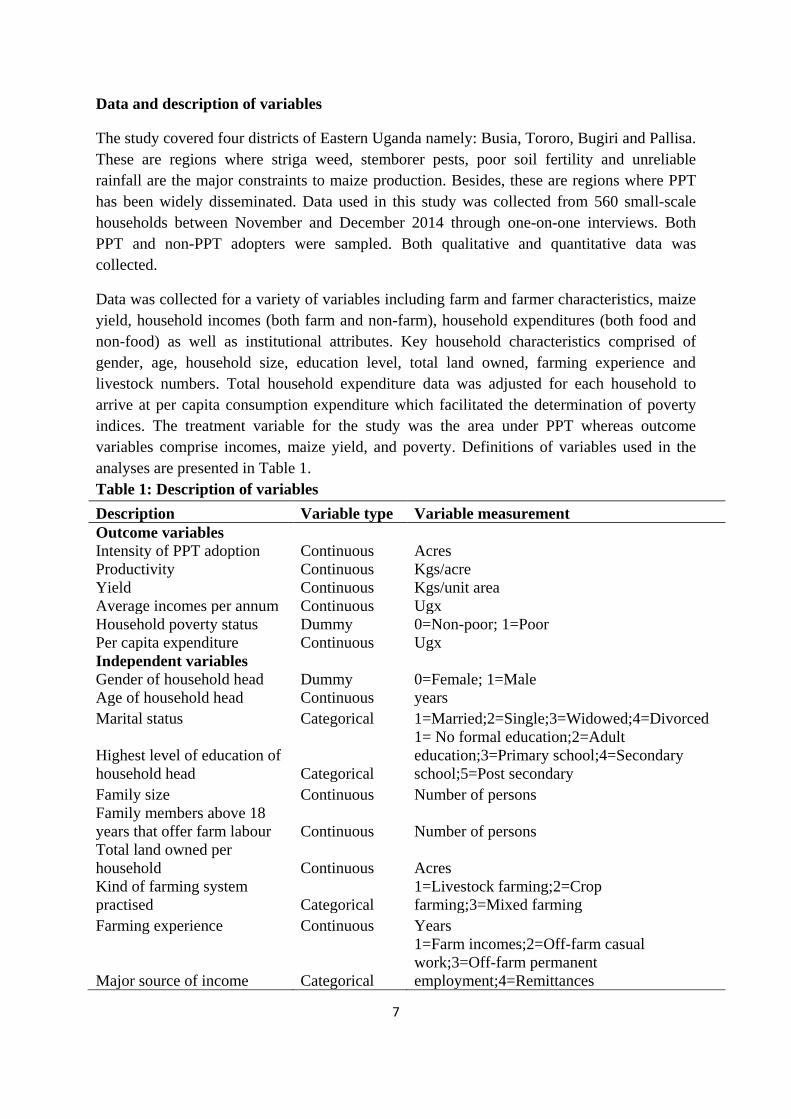
Data and description of variables

The study covered four districts of Eastern Uganda namely: Busia, Tororo, Bugiri and Pallisa.

These are regions where striga weed, stemborer pests, poor soil fertility and unreliable

rainfall are the major constraints to maize production. Besides, these are regions where PPT

has been widely disseminated. Data used in this study was collected from 560 small-scale

households between November and December 2014 through one-on-one interviews. Both

PPT and non-PPT adopters were sampled. Both qualitative and quantitative data was

collected.

Data was collected for a variety of variables including farm and farmer characteristics, maize

yield, household incomes (both farm and non-farm), household expenditures (both food and

non-food) as well as institutional attributes. Key household characteristics comprised of

gender, age, household size, education level, total land owned, farming experience and

livestock numbers. Total household expenditure data was adjusted for each household to

arrive at per capita consumption expenditure which facilitated the determination of poverty

indices. The treatment variable for the study was the area under PPT whereas outcome

variables comprise incomes, maize yield, and poverty. Definitions of variables used in the

analyses are presented in Table 1.

Table 1: Description of variables

Description Variable type Variable measurement

Outcome variables

Intensity of PPT adoption Continuous Acres

Productivity Continuous Kgs/acre

Yield Continuous Kgs/unit area

Average incomes per annum Continuous Ugx

Household poverty status Dummy 0=Non-poor; 1=Poor

Per capita expenditure Continuous Ugx

Independent variables

Gender of household head Dummy 0=Female; 1=Male

Age of household head Continuous years

Marital status Categorical 1=Married;2=Single;3=Widowed;4=Divorced

Highest level of education of

household head Categorical

1= No formal education;2=Adult

education;3=Primary school;4=Secondary

school;5=Post secondary

Family size Continuous Number of persons

Family members above 18

years that offer farm labour Continuous Number of persons

Total land owned per

household Continuous Acres

Kind of farming system

practised Categorical

1=Livestock farming;2=Crop

farming;3=Mixed farming

Farming experience Continuous Years

Major source of income Categorical

1=Farm incomes;2=Off-farm casual

work;3=Off-farm permanent

employment;4=Remittances

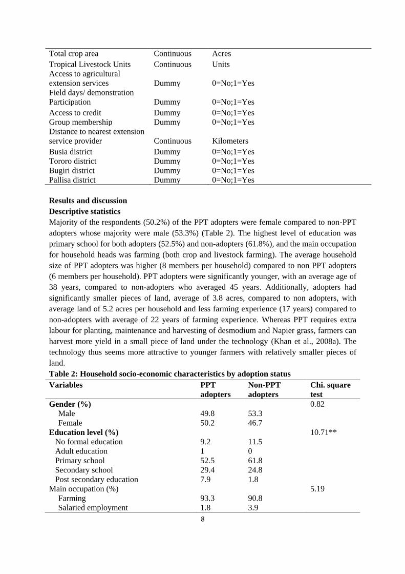
8

Total crop area Continuous Acres

Tropical Livestock Units Continuous Units

Access to agricultural

extension services Dummy 0=No;1=Yes

Field days/ demonstration

Participation Dummy 0=No;1=Yes

Access to credit Dummy 0=No;1=Yes

Group membership Dummy 0=No;1=Yes

Distance to nearest extension

service provider Continuous Kilometers

Busia district Dummy 0=No;1=Yes

Tororo district Dummy 0=No;1=Yes

Bugiri district Dummy 0=No;1=Yes

Pallisa district Dummy 0=No;1=Yes

Results and discussion

Descriptive statistics

Majority of the respondents (50.2%) of the PPT adopters were female compared to non-PPT

adopters whose majority were male (53.3%) (Table 2). The highest level of education was

primary school for both adopters (52.5%) and non-adopters (61.8%), and the main occupation

for household heads was farming (both crop and livestock farming). The average household

size of PPT adopters was higher (8 members per household) compared to non PPT adopters

(6 members per household). PPT adopters were significantly younger, with an average age of

38 years, compared to non-adopters who averaged 45 years. Additionally, adopters had

significantly smaller pieces of land, average of 3.8 acres, compared to non adopters, with

average land of 5.2 acres per household and less farming experience (17 years) compared to

non-adopters with average of 22 years of farming experience. Whereas PPT requires extra

labour for planting, maintenance and harvesting of desmodium and Napier grass, farmers can

harvest more yield in a small piece of land under the technology (Khan et al., 2008a). The

technology thus seems more attractive to younger farmers with relatively smaller pieces of

land.

Table 2: Household socio-economic characteristics by adoption status

Variables PPT

adopters

Non-PPT

adopters

Chi. square

test

Gender (%) 0.82

Male 49.8 53.3

Female 50.2 46.7

Education level (%) 10.71**

No formal education 9.2 11.5

Adult education 1 0

Primary school 52.5 61.8

Secondary school 29.4 24.8

Post secondary education 7.9 1.8

Main occupation (%) 5.19

Farming 93.3 90.8

Salaried employment 1.8 3.9

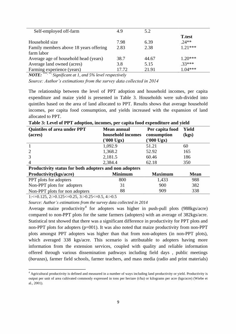
9

Self-employed off-farm 4.9 5.2

T.test

Household size 7.98 6.39 .24**

Family members above 18 years offering

farm labor

2.83 2.38 1.21***

Average age of household head (years) 38.7 44.67 1.20***

Average land owned (acres) 3.8 5.15 .33***

Farming experience (years) 17.72 21.91 1.04*** NOTE: ***, **, Significant at 1, and 5% level respectively

Source: Author’s estimations from the survey data collected in 2014

The relationship between the level of PPT adoption and household incomes, per capita

expenditure and maize yield is presented in Table 3. Households were sub-divided into

quintiles based on the area of land allocated to PPT. Results shows that average household

incomes, per capita food consumption, and yields increased with the expansion of land

allocated to PPT.

Table 3: Level of PPT adoption, incomes, per capita food expenditure and yield

Quintiles of area under PPT

(acres)

Mean annual

household incomes

('000 Ugx)

Per capita food

consumption

('000 Ugx)

Yield

(kgs)

1 1,092.9 51.21 60

2 1,368.2 52.92 165

3 2,181.5 60.46 186

4 2,384.4 62.18 350

Productivity status for both adopters and non adopters

Productivity(kgs/acre) Minimum Maximum Mean

PPT plots for adopters 800 1,433 988

Non-PPT plots for adopters 31 900 382

Non-PPT plots for non adopters 88 909 338

1:<=0.125, 2:>0.125<=0.25, 3:>0.25<=0.5, 4:>0.5

Source: Author’s estimations from the survey data collected in 2014

Average maize productivity4 for adopters was higher in push-pull plots (988kgs/acre)

compared to non-PPT plots for the same farmers (adopters) with an average of 382kgs/acre.

Statistical test showed that there was a significant difference in productivity for PPT plots and

non-PPT plots for adopters (p=001). It was also noted that maize productivity from non-PPT

plots amongst PPT adopters was higher than that from non-adopters (in non-PPT plots),

which averaged 338 kgs/acre. This scenario is attributable to adopters having more

information from the extension services, coupled with quality and reliable information

offered through various dissemination pathways including field days , public meetings

(barazas), farmer field schools, farmer teachers, and mass media (radio and print materials)

4 Agricultural productivity is defined and measured in a number of ways including land productivity or yield. Productivity is

output per unit of area cultivated commonly expressed in tons per hectare (t/ha) or kilograms per acre (kgs/acre) (Wiebe et

al., 2001).

10

used by icipe and extension partners at different stages of dissemination and adoption process

of PPT, and hence, they (adopters) are able to give proper management to even the areas

where PPT is not being applied and get a better crop than the complete non-adopters

(Amudavi et al., 2009; Murage et al., 2011, 2012).

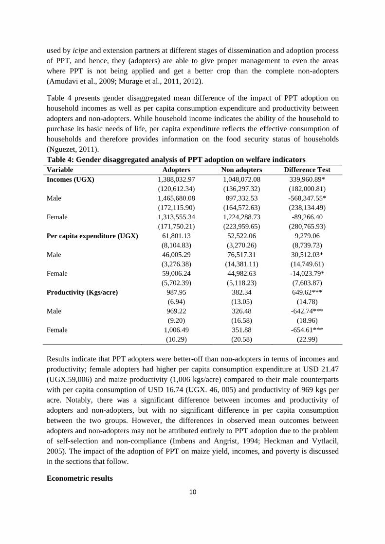
Table 4 presents gender disaggregated mean difference of the impact of PPT adoption on

household incomes as well as per capita consumption expenditure and productivity between

adopters and non-adopters. While household income indicates the ability of the household to

purchase its basic needs of life, per capita expenditure reflects the effective consumption of

households and therefore provides information on the food security status of households

(Nguezet, 2011).

Table 4: Gender disaggregated analysis of PPT adoption on welfare indicators

Variable Adopters Non adopters Difference Test

Incomes (UGX) 1,388,032.97

(120,612.34)

1,048,072.08

(136,297.32)

339,960.89*

(182,000.81)

Male 1,465,680.08

(172,115.90)

897,332.53

(164,572.63)

-568,347.55*

(238,134.49)

Female 1,313,555.34

(171,750.21)

1,224,288.73

(223,959.65)

-89,266.40

(280,765.93)

Per capita expenditure (UGX) 61,801.13

(8,104.83)

52,522.06

(3,270.26)

9,279.06

(8,739.73)

Male 46,005.29

(3,276.38)

76,517.31

(14,381.11)

30,512.03*

(14,749.61)

Female 59,006.24

(5,702.39)

44,982.63

(5,118.23)

-14,023.79*

(7,603.87)

Productivity (Kgs/acre) 987.95

(6.94)

382.34

(13.05)

649.62***

(14.78)

Male 969.22

(9.20)

326.48

(16.58)

-642.74***

(18.96)

Female 1,006.49

(10.29)

351.88

(20.58)

-654.61***

(22.99)

Results indicate that PPT adopters were better-off than non-adopters in terms of incomes and

productivity; female adopters had higher per capita consumption expenditure at USD 21.47

(UGX.59,006) and maize productivity (1,006 kgs/acre) compared to their male counterparts

with per capita consumption of USD 16.74 (UGX. 46, 005) and productivity of 969 kgs per

acre. Notably, there was a significant difference between incomes and productivity of

adopters and non-adopters, but with no significant difference in per capita consumption

between the two groups. However, the differences in observed mean outcomes between

adopters and non-adopters may not be attributed entirely to PPT adoption due to the problem

of self-selection and non-compliance (Imbens and Angrist, 1994; Heckman and Vytlacil,

2005). The impact of the adoption of PPT on maize yield, incomes, and poverty is discussed

in the sections that follow.

Econometric results

11

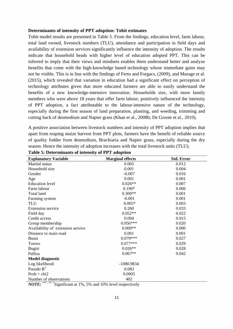
Determinants of intensity of PPT adoption: Tobit estimates

Tobit model results are presented in Table 5. From the findings, education level, farm labour,

total land owned, livestock numbers (TLU), attendance and participation in field days and

availability of extension services significantly influence the intensity of adoption. The results

indicate that household heads with higher level of education adopted PPT. This can be

inferred to imply that their views and mindsets enables them understand better and analyze

benefits that come with the high-knowledge based technology whose immediate gains may

not be visible. This is in line with the findings of Ferto and Forgacs, (2009), and Murage et al.

(2015), which revealed that variation in education had a significant effect on perception of

technology attributes given that more educated farmers are able to easily understand the

benefits of a new knowledge-intensive innovation. Households size, with more family

members who were above 18 years that offer farm labour, positively influenced the intensity

of PPT adoption, a fact attributable to the labour-intensive nature of the technology,

especially during the first season of land preparation, planting, and weeding, trimming and

cutting back of desmodium and Napier grass (Khan et al., 2008b; De Groote et al., 2010).

A positive association between livestock numbers and intensity of PPT adoption implies that

apart from reaping maize harvest from PPT plots, farmers have the benefit of reliable source

of quality fodder from desmodium, Brachiaria and Napier grass, especially during the dry

season. Hence the intensity of adoption increases with the total livestock units (TLU).

Table 5: Determinants of intensity of PPT adoption

Explanatory Variable Marginal effects Std. Error

Marital status 0.005 0.012

Household size 0.001 0.004

Gender -0.007 0.016

Age 0.001 0.001

Education level 0.026** 0.007

Farm labour 0.190* 0.006

Total land 0.300** 0.001

Farming system -0.001 0.001

TLU 0.005* 0.003

Extension service 0.260 0.033

Field day 0.052** 0.022

Credit access 0.004 0.015

Group membership 0.056*** 0.020

Availability of extension service 0.000** 0.000

Distance to main road 0.001 0.001

Busia 0.079*** 0.027

Tororo 0.077*** 0.029

Bugiri 0.026** 0.028

Pallisa 0.067** 0.042

Model diagnostic

Log likelihood -1080.9834

Pseudo R2 0.083

Prob > chi2 0.0005

Number of observations 402

NOTE: *** , **, *Significant at 1%, 5% and 10% level respectively

12

Besides, livestock may also be taken as a proxy of availability of manure which is an efficient

alternative to chemical fertilizers. Results further show that farmers who were in close

contact with agricultural extension officers increased the intensity of PPT adoption. PPT

requires proper crop management practices hence the vital prerequisite of agricultural

extension services. Agricultural extension is the most important source of information to

farmers hence service providers should be able to avail research based information and

educational programs to enable farmers understand a technology, make informed decisions

and implement appropriate knowledge to obtain the best results (Agbamu, 2002; Long and

Sworzel, 2007).

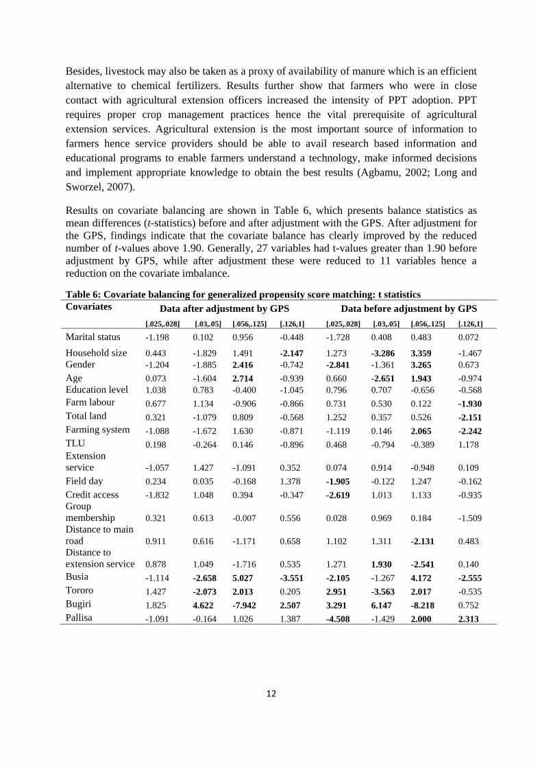
Results on covariate balancing are shown in Table 6, which presents balance statistics as

mean differences (t-statistics) before and after adjustment with the GPS. After adjustment for

the GPS, findings indicate that the covariate balance has clearly improved by the reduced

number of t-values above 1.90. Generally, 27 variables had t-values greater than 1.90 before

adjustment by GPS, while after adjustment these were reduced to 11 variables hence a

reduction on the covariate imbalance.

Table 6: Covariate balancing for generalized propensity score matching: t statistics Covariates Data after adjustment by GPS Data before adjustment by GPS

[.025,.028] [.03,.05] [.056,.125] [.126,1] [.025,.028] [.03,.05] [.056,.125] [.126,1]

Marital status -1.198 0.102 0.956 -0.448 -1.728 0.408 0.483 0.072

Household size 0.443 -1.829 1.491 -2.147 1.273 -3.286 3.359 -1.467

Gender -1.204 -1.885 2.416 -0.742 -2.841 -1.361 3.265 0.673

Age 0.073 -1.604 2.714 -0.939 0.660 -2.651 1.943 -0.974

Education level 1.038 0.783 -0.400 -1.045 0.796 0.707 -0.656 -0.568

Farm labour 0.677 1.134 -0.906 -0.866 0.731 0.530 0.122 -1.930

Total land 0.321 -1.079 0.809 -0.568 1.252 0.357 0.526 -2.151

Farming system -1.088 -1.672 1.630 -0.871 -1.119 0.146 2.065 -2.242

TLU 0.198 -0.264 0.146 -0.896 0.468 -0.794 -0.389 1.178

Extension

service -1.057 1.427 -1.091 0.352 0.074 0.914 -0.948 0.109

Field day 0.234 0.035 -0.168 1.378 -1.905 -0.122 1.247 -0.162

Credit access -1.832 1.048 0.394 -0.347 -2.619 1.013 1.133 -0.935

Group

membership 0.321 0.613 -0.007 0.556 0.028 0.969 0.184 -1.509

Distance to main

road 0.911 0.616 -1.171 0.658 1.102 1.311 -2.131 0.483

Distance to

extension service 0.878 1.049 -1.716 0.535 1.271 1.930 -2.541 0.140

Busia -1.114 -2.658 5.027 -3.551 -2.105 -1.267 4.172 -2.555

Tororo 1.427 -2.073 2.013 0.205 2.951 -3.563 2.017 -0.535

Bugiri 1.825 4.622 -7.942 2.507 3.291 6.147 -8.218 0.752

Pallisa -1.091 -0.164 1.026 1.387 -4.508 -1.429 2.000 2.313

13

Impact of intensity of adoption: Generalized propensity score

The GPS results in Table 7 show that gender, total land owned, participation and/or

attendance of field days, and membership to community organizations had a significant

influence on the intensity of adoption. If a farmer was a member to a community organization

and/ or attended field days, he/she was more likely to gather information about the

technology from other farmers, farmer teachers, and agricultural extension officers and hence

intensified adoption of PPT. Additionally, extension service providers availed technical

advice as well as farm inputs. This agrees with Kassie et al. (2012), who observed that with

scarce or inadequate information sources coupled with imperfect markets and transactions

costs, social networks such as farmers’ associations or groups facilitate the exchange of

information.

Table 7: Estimation of propensity score: Generalized Propensity Score

Explanatory variables Average marginal effects Std. Err

Marital status 0.014 0.074

Household size 0.016 0.022

Gender -0.183* 0.098

Age -0.002 0.005

Education level 0.063 0.042

Farm labour 0.042 0.034

Total land -0.027*** 0.007

Farming system 0.001 0.006

TLU -0.017 0.018

Extension service -0.063 0.209

Field day 0.314** 0.134

Credit access 0.018 0.094

Group membership 0.234* 0.124

Distance to main road 0.003 0.006

Distance to extension service 0.000 0.001

Busia 0.036* 0.129

Tororo 0.105** 0.142

Bugiri 0.605*** 0.178

Pallisa 0.511*** 0.169 NOTE: *** , **, *Significant at 1%, 5% and 10% level respectively

A negative significant relationship of gender means that being female increased the intensity

of PPT adoption. This corroborates the findings of Murage et al. (2015), who observed that a

higher percentage of women perceived PPT as a very effective strategy compared to men, a

fact attributable to the technology characteristics that seemed to favor women's preferences,

and hence more women are likely to intensify adoption than men.

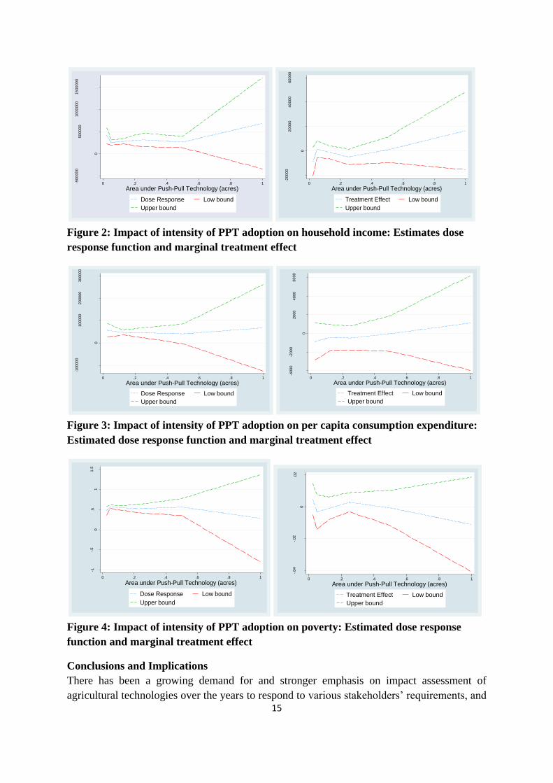
Impact of adoption intensity on welfare outcomes: Dose-response function (DRF)

estimates

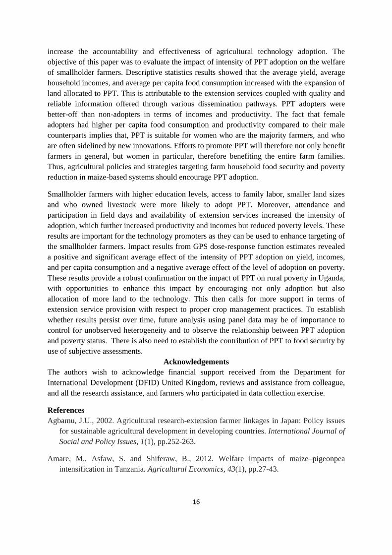
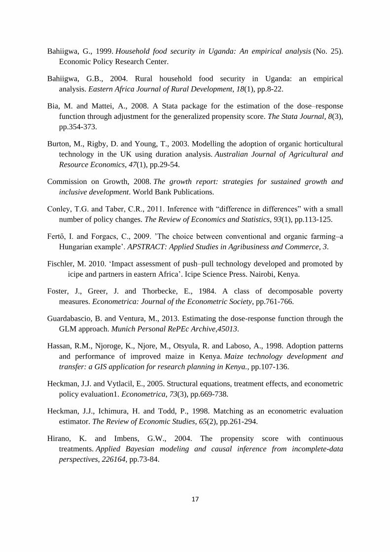
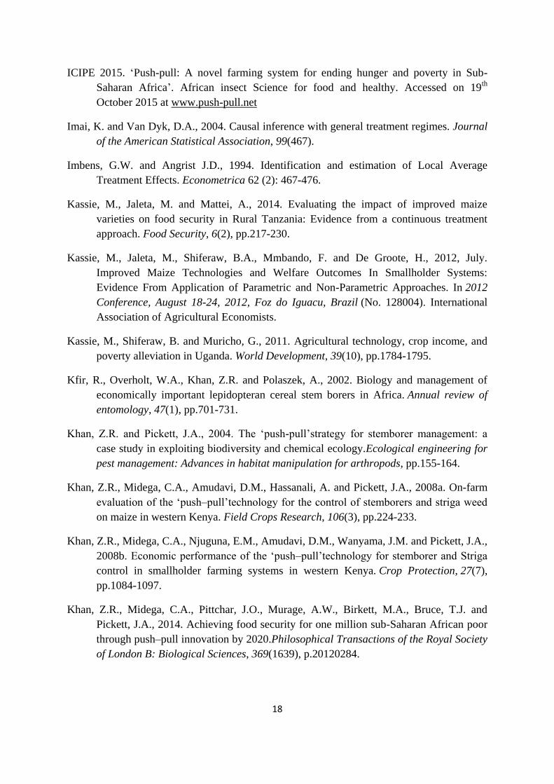
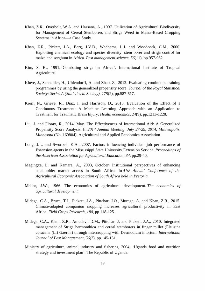
Figures 1 to 4 show the DRF estimates and their derivatives that is the Marginal Treatment

Function (MTF) of the impact of intensity of adoption on maize yield, household incomes,

per capita consumption and poverty. The results clearly depict that there exists a significant

and positive average effect of the intensity of adoption of PPT on maize yield, household

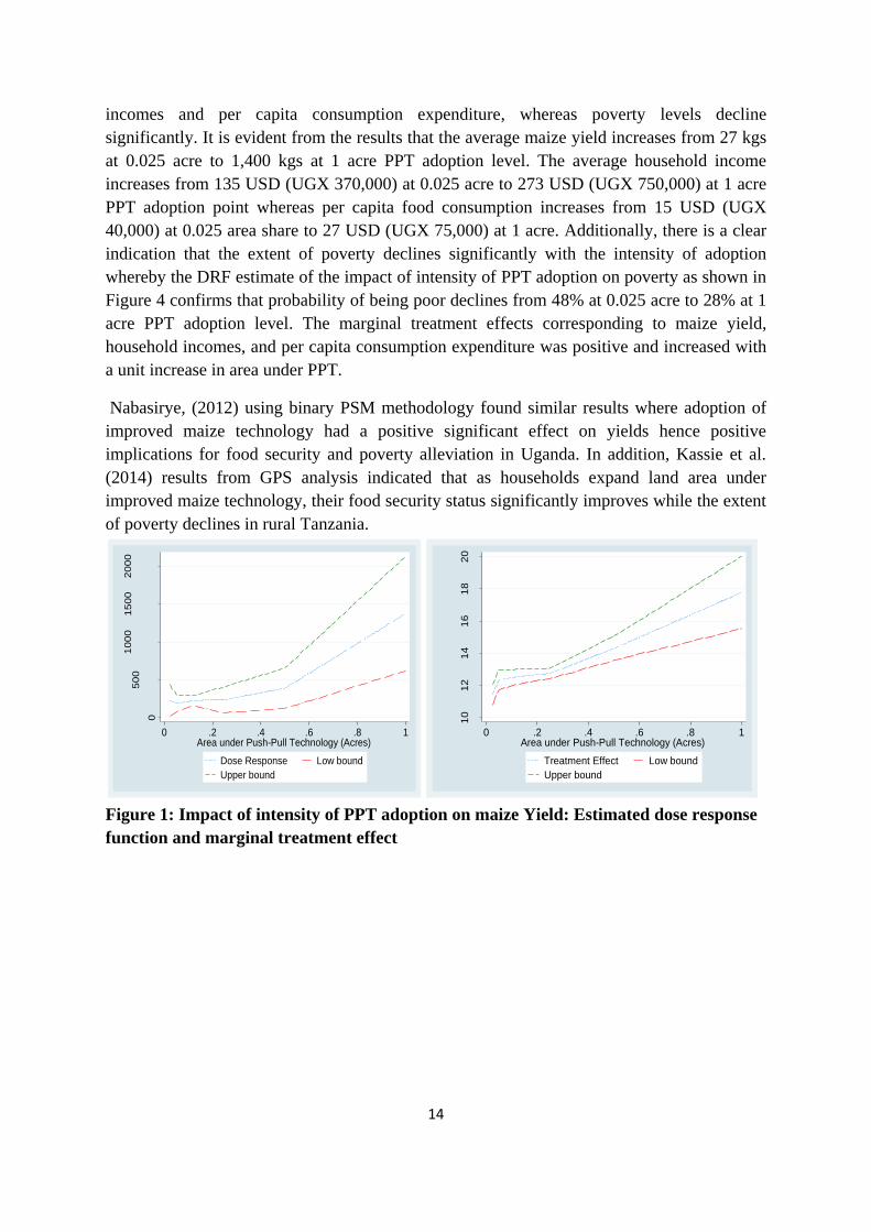
14

incomes and per capita consumption expenditure, whereas poverty levels decline

significantly. It is evident from the results that the average maize yield increases from 27 kgs

at 0.025 acre to 1,400 kgs at 1 acre PPT adoption level. The average household income

increases from 135 USD (UGX 370,000) at 0.025 acre to 273 USD (UGX 750,000) at 1 acre

PPT adoption point whereas per capita food consumption increases from 15 USD (UGX

40,000) at 0.025 area share to 27 USD (UGX 75,000) at 1 acre. Additionally, there is a clear

indication that the extent of poverty declines significantly with the intensity of adoption

whereby the DRF estimate of the impact of intensity of PPT adoption on poverty as shown in

Figure 4 confirms that probability of being poor declines from 48% at 0.025 acre to 28% at 1

acre PPT adoption level. The marginal treatment effects corresponding to maize yield,

household incomes, and per capita consumption expenditure was positive and increased with

a unit increase in area under PPT.

Nabasirye, (2012) using binary PSM methodology found similar results where adoption of

improved maize technology had a positive significant effect on yields hence positive

implications for food security and poverty alleviation in Uganda. In addition, Kassie et al.

(2014) results from GPS analysis indicated that as households expand land area under

improved maize technology, their food security status significantly improves while the extent

of poverty declines in rural Tanzania.

Figure 1: Impact of intensity of PPT adoption on maize Yield: Estimated dose response

function and marginal treatment effect

0

50

01

00

01

50

02

00

0

Yie

ld(K

gs)

0 .2 .4 .6 .8 1Area under Push-Pull Technology (Acres)

Dose Response Low bound

Upper bound

10

12

14

16

18

20

Yie

ld (

Kg

s)

0 .2 .4 .6 .8 1Area under Push-Pull Technology (Acres)

Treatment Effect Low bound

Upper bound

15

Figure 2: Impact of intensity of PPT adoption on household income: Estimates dose

response function and marginal treatment effect

Figure 3: Impact of intensity of PPT adoption on per capita consumption expenditure:

Estimated dose response function and marginal treatment effect

Figure 4: Impact of intensity of PPT adoption on poverty: Estimated dose response

function and marginal treatment effect

Conclusions and Implications

There has been a growing demand for and stronger emphasis on impact assessment of

agricultural technologies over the years to respond to various stakeholders’ requirements, and

-500

00

0

0

50

00

00

10

00

00

015

00

00

0

Ho

use

ho

ld in

co

me

(U

GX

)

0 .2 .4 .6 .8 1

Area under Push-Pull Technology (acres)

Dose Response Low bound

Upper bound

-200

00

0

20

00

040

00

060

00

0

Ho

use

ho

ld in

co

me

(U

GX

)

0 .2 .4 .6 .8 1

Area under Push-Pull Technology (acres)

Treatment Effect Low bound

Upper bound

-100

00

0

0

10

00

00

20

00

00

30

00

00

Pe

r ca

pita

fo

od

co

nsu

mp

tio

n (

UG

X)

0 .2 .4 .6 .8 1

Area under Push-Pull Technology (acres)

Dose Response Low bound

Upper bound

-400

0-2

00

0

0

20

00

40

00

60

00

Pe

r ca

pita

fo

od

co

nsu

mp

tio

n (

UG

X)

0 .2 .4 .6 .8 1

Area under Push-Pull Technology (acres)

Treatment Effect Low bound

Upper bound

-1-.

50

.51

1.5

Po

ve

rty

0 .2 .4 .6 .8 1

Area under Push-Pull Technology (acres)

Dose Response Low bound

Upper bound

-.04

-.02

0

.02

Po

ve

rty

0 .2 .4 .6 .8 1

Area under Push-Pull Technology (acres)

Treatment Effect Low bound

Upper bound

16

increase the accountability and effectiveness of agricultural technology adoption. The

objective of this paper was to evaluate the impact of intensity of PPT adoption on the welfare

of smallholder farmers. Descriptive statistics results showed that the average yield, average

household incomes, and average per capita food consumption increased with the expansion of

land allocated to PPT. This is attributable to the extension services coupled with quality and

reliable information offered through various dissemination pathways. PPT adopters were

better-off than non-adopters in terms of incomes and productivity. The fact that female

adopters had higher per capita food consumption and productivity compared to their male

counterparts implies that, PPT is suitable for women who are the majority farmers, and who

are often sidelined by new innovations. Efforts to promote PPT will therefore not only benefit

farmers in general, but women in particular, therefore benefiting the entire farm families.

Thus, agricultural policies and strategies targeting farm household food security and poverty

reduction in maize-based systems should encourage PPT adoption.

Smallholder farmers with higher education levels, access to family labor, smaller land sizes

and who owned livestock were more likely to adopt PPT. Moreover, attendance and

participation in field days and availability of extension services increased the intensity of

adoption, which further increased productivity and incomes but reduced poverty levels. These

results are important for the technology promoters as they can be used to enhance targeting of

the smallholder farmers. Impact results from GPS dose-response function estimates revealed

a positive and significant average effect of the intensity of PPT adoption on yield, incomes,

and per capita consumption and a negative average effect of the level of adoption on poverty.

These results provide a robust confirmation on the impact of PPT on rural poverty in Uganda,

with opportunities to enhance this impact by encouraging not only adoption but also

allocation of more land to the technology. This then calls for more support in terms of

extension service provision with respect to proper crop management practices. To establish

whether results persist over time, future analysis using panel data may be of importance to

control for unobserved heterogeneity and to observe the relationship between PPT adoption

and poverty status. There is also need to establish the contribution of PPT to food security by

use of subjective assessments.

Acknowledgements

The authors wish to acknowledge financial support received from the Department for

International Development (DFID) United Kingdom, reviews and assistance from colleague,

and all the research assistance, and farmers who participated in data collection exercise.

References

Agbamu, J.U., 2002. Agricultural research-extension farmer linkages in Japan: Policy issues

for sustainable agricultural development in developing countries. International Journal of

Social and Policy Issues, 1(1), pp.252-263.

Amare, M., Asfaw, S. and Shiferaw, B., 2012. Welfare impacts of maize–pigeonpea

intensification in Tanzania. Agricultural Economics, 43(1), pp.27-43.

17

Bahiigwa, G., 1999. Household food security in Uganda: An empirical analysis (No. 25).

Economic Policy Research Center.

Bahiigwa, G.B., 2004. Rural household food security in Uganda: an empirical

analysis. Eastern Africa Journal of Rural Development, 18(1), pp.8-22.

Bia, M. and Mattei, A., 2008. A Stata package for the estimation of the dose–response

function through adjustment for the generalized propensity score. The Stata Journal, 8(3),

pp.354-373.

Burton, M., Rigby, D. and Young, T., 2003. Modelling the adoption of organic horticultural

technology in the UK using duration analysis. Australian Journal of Agricultural and

Resource Economics, 47(1), pp.29-54.

Commission on Growth, 2008. The growth report: strategies for sustained growth and

inclusive development. World Bank Publications.

Conley, T.G. and Taber, C.R., 2011. Inference with “difference in differences” with a small

number of policy changes. The Review of Economics and Statistics, 93(1), pp.113-125.

Fertő, I. and Forgacs, C., 2009. ’The choice between conventional and organic farming–a

Hungarian example’. APSTRACT: Applied Studies in Agribusiness and Commerce, 3.

Fischler, M. 2010. ‘Impact assessment of push–pull technology developed and promoted by

icipe and partners in eastern Africa’. Icipe Science Press. Nairobi, Kenya.

Foster, J., Greer, J. and Thorbecke, E., 1984. A class of decomposable poverty

measures. Econometrica: Journal of the Econometric Society, pp.761-766.

Guardabascio, B. and Ventura, M., 2013. Estimating the dose-response function through the

GLM approach. Munich Personal RePEc Archive,45013.

Hassan, R.M., Njoroge, K., Njore, M., Otsyula, R. and Laboso, A., 1998. Adoption patterns

and performance of improved maize in Kenya. Maize technology development and

transfer: a GIS application for research planning in Kenya., pp.107-136.

Heckman, J.J. and Vytlacil, E., 2005. Structural equations, treatment effects, and econometric

policy evaluation1. Econometrica, 73(3), pp.669-738.

Heckman, J.J., Ichimura, H. and Todd, P., 1998. Matching as an econometric evaluation

estimator. The Review of Economic Studies, 65(2), pp.261-294.

Hirano, K. and Imbens, G.W., 2004. The propensity score with continuous

treatments. Applied Bayesian modeling and causal inference from incomplete-data

perspectives, 226164, pp.73-84.

18

ICIPE 2015. ‘Push-pull: A novel farming system for ending hunger and poverty in Sub-

Saharan Africa’. African insect Science for food and healthy. Accessed on 19th

October 2015 at www.push-pull.net

Imai, K. and Van Dyk, D.A., 2004. Causal inference with general treatment regimes. Journal

of the American Statistical Association, 99(467).

Imbens, G.W. and Angrist J.D., 1994. Identification and estimation of Local Average

Treatment Effects. Econometrica 62 (2): 467-476.

Kassie, M., Jaleta, M. and Mattei, A., 2014. Evaluating the impact of improved maize

varieties on food security in Rural Tanzania: Evidence from a continuous treatment

approach. Food Security, 6(2), pp.217-230.

Kassie, M., Jaleta, M., Shiferaw, B.A., Mmbando, F. and De Groote, H., 2012, July.

Improved Maize Technologies and Welfare Outcomes In Smallholder Systems:

Evidence From Application of Parametric and Non-Parametric Approaches. In 2012

Conference, August 18-24, 2012, Foz do Iguacu, Brazil (No. 128004). International

Association of Agricultural Economists.

Kassie, M., Shiferaw, B. and Muricho, G., 2011. Agricultural technology, crop income, and

poverty alleviation in Uganda. World Development, 39(10), pp.1784-1795.

Kfir, R., Overholt, W.A., Khan, Z.R. and Polaszek, A., 2002. Biology and management of

economically important lepidopteran cereal stem borers in Africa. Annual review of

entomology, 47(1), pp.701-731.

Khan, Z.R. and Pickett, J.A., 2004. The ‘push-pull’strategy for stemborer management: a

case study in exploiting biodiversity and chemical ecology.Ecological engineering for

pest management: Advances in habitat manipulation for arthropods, pp.155-164.

Khan, Z.R., Midega, C.A., Amudavi, D.M., Hassanali, A. and Pickett, J.A., 2008a. On-farm

evaluation of the ‘push–pull’technology for the control of stemborers and striga weed

on maize in western Kenya. Field Crops Research, 106(3), pp.224-233.

Khan, Z.R., Midega, C.A., Njuguna, E.M., Amudavi, D.M., Wanyama, J.M. and Pickett, J.A.,

2008b. Economic performance of the ‘push–pull’technology for stemborer and Striga

control in smallholder farming systems in western Kenya. Crop Protection, 27(7),

pp.1084-1097.

Khan, Z.R., Midega, C.A., Pittchar, J.O., Murage, A.W., Birkett, M.A., Bruce, T.J. and

Pickett, J.A., 2014. Achieving food security for one million sub-Saharan African poor

through push–pull innovation by 2020.Philosophical Transactions of the Royal Society

of London B: Biological Sciences, 369(1639), p.20120284.

19

Khan, Z.R., Overholt, W.A. and Hassana, A., 1997. Utilization of Agricultural Biodiversity

for Management of Cereal Stemborers and Striga Weed in Maize-Based Cropping

Systems in Africa—a Case Study.

Khan, Z.R., Pickett, J.A., Berg, J.V.D., Wadhams, L.J. and Woodcock, C.M., 2000.

Exploiting chemical ecology and species diversity: stem borer and striga control for

maize and sorghum in Africa. Pest management science, 56(11), pp.957-962.

Kim, S. K., 1991. ‘Combating striga in Africa’. International Institute of Tropical

Agriculture.

Kluve, J., Schneider, H., Uhlendorff, A. and Zhao, Z., 2012. Evaluating continuous training

programmes by using the generalized propensity score. Journal of the Royal Statistical

Society: Series A (Statistics in Society), 175(2), pp.587-617.

Kreif, N., Grieve, R., Díaz, I. and Harrison, D., 2015. Evaluation of the Effect of a

Continuous Treatment: A Machine Learning Approach with an Application to

Treatment for Traumatic Brain Injury. Health economics, 24(9), pp.1213-1228.

Liu, J. and Florax, R., 2014, May. The Effectiveness of International Aid: A Generalized

Propensity Score Analysis. In 2014 Annual Meeting, July 27-29, 2014, Minneapolis,

Minnesota (No. 169804). Agricultural and Applied Economics Association.

Long, J.L. and Swortzel, K.A., 2007. Factors influencing individual job performance of

Extension agents in the Mississippi State University Extension Service. Proceedings of

the American Association for Agricultural Education, 34, pp.29-40.

Magingxa, L. and Kamara, A., 2003, October. Institutional perspectives of enhancing

smallholder market access in South Africa. In 41st Annual Conference of the

Agricultural Economic Association of South Africa held in Pretoria.

Mellor, J.W., 1966. The economics of agricultural development. The economics of

agricultural development.

Midega, C.A., Bruce, T.J., Pickett, J.A., Pittchar, J.O., Murage, A. and Khan, Z.R., 2015.

Climate-adapted companion cropping increases agricultural productivity in East

Africa. Field Crops Research, 180, pp.118-125.

Midega, C.A., Khan, Z.R., Amudavi, D.M., Pittchar, J. and Pickett, J.A., 2010. Integrated

management of Striga hermonthica and cereal stemborers in finger millet (Eleusine

coracana (L.) Gaertn.) through intercropping with Desmodium intortum. International

Journal of Pest Management, 56(2), pp.145-151.

Ministry of agriculture, animal industry and fisheries, 2004. ‘Uganda food and nutrition

strategy and investment plan’. The Republic of Uganda.

20

Mukhebi, A., Mbogoh, S., & Matungulu, K., 2011.’ An overview of the food security

situation in eastern Africa’. Economic commission for Africa sub-regional office for

eastern Africa.

Murage, A.W., Amudavi, D.M., Obare, G., Chianu, J., Midega, C.A.O., Pickett, J.A. and

Khan, Z.R., 2011. Determining smallholder farmers' preferences for technology

dissemination pathways: the case of ‘push–pull’technology in the control of stemborer

and Striga weeds in Kenya.International Journal of Pest Management, 57(2), pp.133-

145.

Murage, A.W., Obare, G., Chianu, J., Amudavi, D.M., Midega, C.A.O., Pickett, J.A. and

Khan, Z.R., 2012. The Effectiveness of Dissemination Pathways on Adoption of"

Push-Pull" Technology in Western Kenya.Quarterly Journal of International

Agriculture, 51(1), p.51.

Murage, A.W., Pittchar, J.O., Midega, C.A.O., Onyango, C.O. and Khan, Z.R., 2015. Gender

specific perceptions and adoption of the climate-smart push–pull technology in eastern

Africa. Crop Protection, 76, pp.83-91.

Musselman, L.J., Safa, S.B., Knepper, D.A., Mohamed, K.I., White, C.L. and Kim, S.K.,

1991. Recent research on the biology of Striga asiatica, S. gesnerioides and S.

hermonthica. In Combating striga in Africa: proceedings of the international workshop

held in Ibadan, Nigeria, 22-24 August 1988. (pp. 31-41). International Institute of

Tropical Agriculture.

Nabasirye, M., Kiiza, B. and Omiat, G., 2012. Evaluating the Impact of Adoption of

Improved Maize Varieties on Yield in Uganda: A Propensity Score Matching

Approach. Journal of Agricultural Science and Technology. B, 2(3B), p.368.

Ouma, J., Bett, E., & Mbataru, P., 2014. Does Adoption of Improved Maize Varieties

Enhance Household Food Security in Maize growing Zones of Eastern Kenya.

Developing Country Studies, 4(23), 157-165.

Romney, D.L., Thorne, P., Lukuyu, B. and Thornton, P.K., 2003. Maize as food and feed in

intensive smallholder systems: management options for improved integration in mixed

farming systems of east and southern Africa.Field crops research, 84(1), pp.159-168.

Rosenbaum, P.R. and Rubin, D.B., 1983. The central role of the propensity score in

observational studies for causal effects. Biometrika, 70(1), pp.41-55.

Rosenbaum, P.R. and Rubin, D.B., 1985. Constructing a control group using multivariate

matched sampling methods that incorporate the propensity score. The American

Statistician, 39(1), pp.33-38.

Rubin, D.B., 2005. Causal inference using potential outcomes. Journal of the American

Statistical Association 100 (469):322–331.

21

Salami, A., Kamara, A.B. and Brixiova, Z., 2010. Smallholder agriculture in East Africa:

trends, constraints and opportunities. Tunis, Tunisia: African Development Bank.

Simtowe, F., Kassie, M., Asfaw, S., Shiferaw, B., Monyo, E. and Siambi, M., 2012, August.

Welfare Effects of Agricultural Technology adoption: the case of improved groundnut

varieties in rural Malawi. In Selected Paper prepared for presentation at the

International Association of Agricultural Economists (IAAE) Triennial Conference,

Foz do Iguaçu, Brazil (pp. 18-24).

Smil, V., 2001. Feeding the world: A challenge for the twenty-first century. MIT press.

Ssewanyana, S. and Kasirye, I., 2010. Food insecurity in Uganda: a dilemma to achieving the

hunger millennium development goal.