IMPACT ASSESSMENT STUDY OF ASSISTED MICRO FINANCE

IMPACT ASSESSMENT STUDY OF ASSISTED MICRO FINANCE INSTITUTIONS UNDER

“SCALING UP SUSTAINABLE AND RESPONSIBLE MICRO FINANCE

PROJECT”

Baseline Report

March 2013

Submitted to

Small Industries Development Bank of India Scaling Up Sustainable and Responsible Microfinance Project

SIDBI Tower, 15, Ashok Marg, Lucknow-226001, Uttar Pradesh, India

Submitted by

Catalyst Management Services Private Limited (Lead Firm) Head Office: No. 19, 1

st Main, 1

st Cross, Aswath Nagar, RMV II Stage, Bangalore – 560 094, India

Ph: + 91 80 2341 9616 Email: [email protected]; [email protected]; Web: http://www.cms.org.in Branch Offices at - New Delhi, Bhopal, Bhubaneshwar, Hyderabad, Madurai and Phnom Penh (Cambodia)

mailto:[email protected]

mailto:[email protected]

http://www.cms.org.in/

Contents

Summary .................................................................................................................................. 4

1 Introduction ....................................................................................................................... 9

2 The Scaling Up Sustainable and Responsible Micro Finance Project ................... 9

2.1 About the project ....................................................................................................... 9

2.2 The Project Theory of Change ............................................................................. 10

3 Impact Evaluation: Design and Methods ................................................................... 13

3.1 Objectives and key questions of the Impact Evaluation ................................... 14

3.2 Expectations from the Impact Evaluation ........................................................... 14

3.3 Framework for Assessing Impact at End-User Client Level – Mixed-Method Design ................................................................................................................................. 16

3.4 Quantitative Design ................................................................................................ 17

3.4.1 MFI Sampling: Challenges and decisions ................................................... 17

3.4.2 Sampling of Clients ......................................................................................... 19

3.4.3 Sources of Information, Tools and Methods ............................................... 22

3.5 Qualitative Design .................................................................................................. 22

3.5.1 Objective and information needs from FGDs (at the Baseline) ............... 22

3.5.2 Sampling ........................................................................................................... 23

3.6 Evaluation Model and Analytical Framework ..................................................... 24

4 Baseline Results: The RCT Study .............................................................................. 26

4.1 Profile of Samples .................................................................................................. 26

4.2 Impact Indicators .................................................................................................... 30

4.2.1 Multidimensional Poverty Index .................................................................... 30

4.2.2 Progress out of Poverty Index ....................................................................... 33

4.2.3 Women Empowerment Score ....................................................................... 35

4.3 Outcome Indicators ................................................................................................ 38

4.3.1 Household Income and Expenditure ............................................................ 38

4.3.2 Enterprises ....................................................................................................... 43

4.4 Financial Indicators ................................................................................................ 45

4.4.1 Financial Literacy ............................................................................................ 45

4.4.2 Savings ............................................................................................................. 46

4.4.3 Credit ................................................................................................................. 48

4.4.4 Investment in Enterprise ................................................................................ 62

5 Baseline Results: The Non-RCT Study ..................................................................... 64

5.1 Profile of Samples .................................................................................................. 64

5.2 Impact Indicators .................................................................................................... 65

5.2.1 Multidimensional Poverty Index .................................................................... 66

5.2.2 Progress out of Poverty Index ....................................................................... 67

5.2.3 Women Empowerment Score ....................................................................... 69

5.3 Outcome Indicators ................................................................................................ 71

5.3.1 Household Income and Expenditure ............................................................ 71

5.3.2 Enterprises ....................................................................................................... 76

5.4 Financial Indicators ................................................................................................ 78

5.4.1 Financial Literacy ............................................................................................ 78

5.4.2 Savings ............................................................................................................. 79

5.4.3 Credit ................................................................................................................. 81

5.4.4 Investment in Enterprise ................................................................................ 92

6 Key messages from the baseline study (RCT and non-RCT) ................................ 95

Annexure A: Timelines and discussions on MFI selection ............................................. 96

SUMMARY The “Scaling Up Sustainable and Responsible Micro Finance Project” is a World Bank supported project, with the objective to scale up access to sustainable microfinance services to the financially excluded, particularly in under-served areas of India, through, among other things, introduction of innovative financial products and fostering transparency and responsible finance. The project Theory of Change identifies the issues at the baseline: namely, poverty and marginalization which lead to poor access to services, lack skills and capacities to access and optimally employ credit, caste and structural issues and lack of formal institutions. The project brings in financial products, capacity development, business development services and institutional development services, expected to improve outreach, increase the products accessed and improve the MFI performance and satisfaction of clients. At the client end the initiative seeks to bring changes in the cognitive and perceptual abilities (financial literacy and discipline, risk taking, etc.), economic and material status, basic survival status and women’s empowerment. The long term, wider social impact is improved education, improved position of women and girls in society, improved credit market with better services from banks and MFIs and greater market access by women, and finally greater political meaningful participation by women. A graphic representation of the Theory of Change is given below

An impact evaluation was commissioned by World Bank and SIDBI to measure the impact of the project, and the attributability of the change to the project. Catalyst Management Services Pvt. Ltd. led a team of researchers and evaluators in conducting the study. This is the report of the baseline of the study.

Financial Products: Credit, Insurance, Savings

Capacity Development (Financial Literacy)

Business Development Services (Training, Market

linkages, Others)

Institutional Development Services (Community

institution, Federations, Capacity building)

Outreach:

- Clients Reached (women, SC/ST, diabled, Rural, Urban..) - Socio-economic profile - Geographical spread

Product Access: - Products offered - Size and growth - Outstanding loans

MFI Performance: - Repayment status - Frequency of repayment

Client Satisfaction: - Clients understanding - Satisfaction (timeliness, size, services)

Context/ Problems or Issues

Addressed Products and Services by

MFIs to Bring Change Results/ Outputs of MFI

(MFI Performance) Immediate Outcomes of

MFI Strategy (Direct, Short-

Medium or Long term

Outcomes and Impact

Cognitive/ Perceptual: - Financial literacy - Planning for life - Financial discipline - Ability to face risk - Behaviour to save

Economic/ Material: - Enterprise turnover - Cost of production - Assets redemption - Access to land, assets - Loan Utilisation pattern - Level of indebtedness - Reduced distress migration - Reduced informal credit

Basic Survival & Services:: - Food security - Diversity of diet - Better health, education - Better clothing, housing

Positional Impact: - Women's control over loan - Assets in women's name - Reduced domestic violence - Women's position in family

Wider Social Impact: - Women in public space - Women in community decisions - Girl children in schools - Increased enrolment - HIgher education - Community institutions addressing issues

Wider Market Impact:

- More women in business - Reduced interest rates - Better service from banks - Better policies

Political Impact:

- Participation in local governance/ politics

THEORY OF CHANGE - PATHWAY TO IMPACT FINANCIAL PRODUCTS AND SERVICES -------> TO -----------> ECONOMIC, SOCIAL AND POLITICAL OUTCOMES AND IMPACT OF MFI CLIENTS

Access to Services

- Poor Access to Financial Services - Lack of access to Markets - Geographical isolation

Skills and Capacities

- Illiteracy - Lack of financial literacy - Low assets and risk taking ability - No fall back mechanisms

Caste and Structural Issues: - Exclusion s due to caste, gender, religion and geography backwardness - No voice politically

Lack of Formal Insitutions

- Informal instiuttions - Informal systems

Overall - Poverty and

Marginalisation

MFI Delivery Models - SHG-Federation, Grameen, Individual Banking, Sector Spcific Models; Geography - Across India/ Four Regions + North East; Varying Scales of Reach and Varying Loan Sizes; Varying Products; Rural and Urban

The central objective of the impact evaluation of the Project was to:

Assess programme outcomes and impact

Understand how these outcomes and impact were achieved

Identify the role of MFI partners/ SIDBI in achieving these

Provide recommendations on how to improve the quality and delivery of financial and non-financial products and services offered to clients by MFIs

Document and share good practices and lessons learnt in terms of strategies adopted to achieve the objectives of micro finance

Flowing from this central objective, the key questions of the impact evaluation at various levels were identified. At the Client Level: 1) What profile of communities that partner MFIs reach out – (a) the economically and socially marginalized groups (poor, women, SC/ST/OBC, disabled, other vulnerable groups) and (b) others?, also by type of geography (rural/ urban); 2) What are the outcomes and impact created among the end users of micro finance, due to services provided by MFIs? Are these impacts as envisaged? 3) Do ultimate borrowers in different locations (including underserved and un-served areas) experience responsible microfinance practices, and to what extent? 4) Are there any negative impacts at various levels due to MFI products and services? At the MFI Level: 1) To what extent have institutions in the micro finance sector (SIBDI, its partner MFIs and other lenders) adopted and are practicing responsible and sustainable microfinance practices?

Methodology A quasi-experimental, mixed method design was framed for the impact evaluation. A sample of 4,200 households across 5 MFIs was drawn for the study The quasi-experimental design involved a phase-in approach, wherein the sample would equally divided into 3 groups, with one group receiving the intervention for 3 years, one group for 2 years and the last group for 1 year. This would provide a counterfactual for comparison. Due to challenges faced by the sampled MFIs, four MFIs form the original list were replaced, and of these two were studied through a non-experimental, before-after design. As such the study is divided into two parts, referred to in this report as RCT and non-RCT study. The total sample for the study is as follows:

SNo MFI covered State Sample Covered Comparison

RCT samples

1 Equitas MP 840 Yes

2 Margdarhak UP 840 Yes

3 Sangamitra Mah 840 Yes

Non-RCT samples

4 Sonata Karnataka, UP, Uttarakhand

840 No

5 Janalakshmi 840 No

Total 4,200

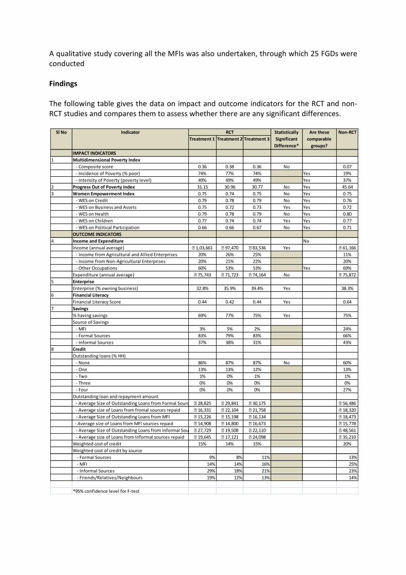
A qualitative study covering all the MFIs was also undertaken, through which 25 FGDs were conducted Findings The following table gives the data on impact and outcome indicators for the RCT and non-RCT studies and compares them to assess whether there are any significant differences.

Treatment 1 Treatment 2 Treatment 3

IMPACT INDICATORS

1 Multidimensional Poverty Index

- Composite score 0.36 0.38 0.36 No 0.07

- Incidence of Poverty (% poor) 74% 77% 74% Yes 19%

- Intensity of Poverty (poverty level) 49% 49% 49% Yes 37%

2 Progress Out of Poverty Index 31.15 30.96 30.77 No Yes 45.64

3 Women Empowerment Index 0.75 0.74 0.75 No Yes 0.75

- WES on Credit 0.79 0.78 0.79 No Yes 0.76

- WES on Business and Assets 0.75 0.72 0.73 Yes Yes 0.72

- WES on Health 0.79 0.78 0.79 No Yes 0.80

- WES on Children 0.77 0.74 0.74 Yes Yes 0.77

- WES on Political Participation 0.66 0.66 0.67 No Yes 0.71

OUTCOME INDICATORS

4 Income and Expenditure No

Income (annual average) ₹ 1,03,661 ₹ 97,470 ₹ 83,536 Yes ₹ 61,166

- Income from Agricultural and Allied Enterprises 20% 26% 25% 11%

- Income from Non-Agricultural Enterprises 20% 21% 22% 20%

- Other Occupations 60% 53% 53% Yes 69%

Expenditure (annual average) ₹ 75,743 ₹ 71,723 ₹ 74,164 No ₹ 75,872

5 Enterprise

Enterprise (% owning business) 32.8% 35.9% 39.4% Yes 38.3%

6 Financial Literacy

Financial Literacy Score 0.44 0.42 0.44 Yes 0.64

7 Savings

% having savings 69% 77% 75% Yes 75%

Source of Savings

- MFI 3% 5% 2% 24%

- Formal Sources 83% 79% 83% 66%

- Informal Sources 37% 38% 31% 43%

8 Credit

Outstanding loans (% HH)

- None 86% 87% 87% No 60%

- One 13% 13% 12% 13%

- Two 1% 0% 1% 1%

- Three 0% 0% 0% 0%

- Four 0% 0% 0% 27%

Outstanding loan and repayment amount

- Average Size of Outstanding Loans from Formal Sources₹ 28,825 ₹ 29,841 ₹ 30,175 ₹ 56,486

- Average size of Loans from fromal sources repaid ₹ 16,331 ₹ 22,104 ₹ 21,758 ₹ 18,320

- Average Size of Outstanding Loans from MFI ₹ 15,226 ₹ 15,198 ₹ 16,134 ₹ 18,473

- Average size of Loans from MFI sources repaid ₹ 14,908 ₹ 14,800 ₹ 16,673 ₹ 15,778

- Average Size of Outstanding Loans from Informal Sources₹ 27,729 ₹ 19,508 ₹ 22,110 ₹ 48,561

- Average size of Loans from Informal sources repaid ₹ 19,645 ₹ 17,121 ₹ 24,098 ₹ 35,210

Weighted cost of credit 15% 14% 15% 20%

Weighted cost of credit by source

- Formal Sources 9% 8% 11% 13%

- MFI 14% 14% 16% 25%

- Informal Sources 29% 18% 21% 23%

- Friends/Relatives/Neighbours 19% 12% 13% 14%

*95% confidence level for F-test

RCT Non-RCTSl No Indicator Are these

comparable

groups?

Statistically

Significant

Difference*

This table presents the tests of balance for the RCT component of the study. It looks at baseline status of certain key profile indicators to see if the treatment groups are comparable or not.

The groups are comparable on 2 of the listed indicators. However, the quantum of differences as seen from the average or % values is not very large. There is a significant difference in the average annual incomes of the three groups. Key message from the baseline The baseline study has established the status of the impact, outcome and program indicators for different samples The baseline indicates that:

The project is target profiles that are deserving, given the status of impact indicators

Level of financial literacy low

Current level of access to credit seems limited; also the institutional credit

Cost of credit ranges widely; goes up to 10% p.m.

Level of access to insurance also low

Treatment 1 Treatment 2 Treatment 3

9 Primary Occupation of the Household Yes No

- Agriculture 21% 24% 23%

- Artisnal 2% 3% 4%

- Govt. or Pvt. Service 8% 7% 7%

- Labour 45% 41% 42%

- Livestock and Fishery 2% 3% 5%

- Others 7% 4% 5%

- Petty Shops 10% 13% 12%

- Trading and Vending 5% 4% 4%

10 Average Annual Income ₹ 1,03,661 ₹ 97,470 ₹ 82,535 Yes No

11 Average Annual Expenditure ₹ 75,743 ₹ 71,723 ₹ 74,164 No Yes

12 Social Groups Yes No

- Scheduled Caste 31% 26% 30%

- Scheduled Tribe 3% 5% 6%

- Other Backward Caste 42% 39% 43%

- Others 22% 27% 21%

- Don’t want to Answer 1% 1% 1%

13 Religion Yes No

- Hindu 83% 79% 82%

- Muslim 16% 20% 17%

- Christian 0% 0% 1%

- Sikh 0% 1% 0%

- Others 1% 0% 0%

14 Gender of the Head of the Household No Yes

- Male 92% 92% 90%

- Female 8% 8% 10%

- Other 1% 0% 0%

15 Type of Housing Yes No

- Pucca 30% 29% 25%

- Semi-Pucca 47% 45% 44%

- Kutcha 23% 25% 31%

*95% confidence level

Sl No Indicator RCT Statistically

Significant

Are these

comparable

MFI is the preferred source for credit for enterprise but quantum of loans available from MFI is small, and loans are not necessarily structured to meet the credit needs of the poor. They are still compelled to depend on informal sources for their needs. Grievance mechanisms not completely developed. This results in some suspicion, especially if there is a feeling of being cheated. Towards this greater communication and frequent financial literacy related activities are required. Satisfaction with MFI is moderate, particularly on flexibility of repayment and credit limit. This also prevents people from using MFI for enterprises that do not have regular and periodic returns from enterprise.

1 INTRODUCTION

The Indian microfinance sector witnessed tremendous growth between 2005-10, during which time institutions were subject to little regulation. Some microfinance institutions were subject to prudential requirements; however there was no regulation that addressed lending practices, pricing, or operations. The combination of minimal regulation and rapid sector growth led to an environment where customers were increasingly dissatisfied with microfinance services, culminating in the Andhra Pradesh crisis in the fall of 2010 that caused huge losses due to very poor repayments by clients. The crisis soon spiraled nationally, bringing the sector to a standstill1. This situation was further exacerbated by the global financial crisis. The Reserve Bank of India (RBI) responded by appointing an RBI sub-committee know as the Malegam Committee. The consequent draft Microfinance Bill, 2011 sought regulation of the sector. As a result of these events, the outreach of the MFIs was getting curtailed and there were many changes happening at various levels - policy, program and grass-root. Despite the turmoil in the sector, the need for financial services and development support at the bottom of the pyramid (BOP segment) continued to be recognized as a critical input for improving productivity and incomes, as was the need to make microfinance available effectively, sustainably and responsibly.

2 THE SCALING UP SUSTAINABLE AND RESPONSIBLE MICRO FINANCE

PROJECT

2.1 About the project

The “Scaling Up Sustainable and Responsible Micro Finance Project” is a World Bank supported project, with the objective to scale up access to sustainable microfinance services to the financially excluded, particularly in under-served areas of India, through, among other things, introduction of innovative financial products and fostering transparency and responsible finance. From the experiences, it is expected that improved access to finance would help contribute to household asset creation and sustainable income generation, poverty reduction and growth. The Project is being implemented by SIDBI through SIDBI Foundation for Microcredit (SFMC), a specialized department for carrying out micro finance activities. The Scaling Up Project was designed, with a clear objective of scaling up only sustainable and responsible micro finance initiatives in India. The idea was to build on the supported MFIs in the previous phase of the SIDBI’s micro finance program. Given the context, the Scale up Project was designed to have three components:

1 Microfinance in India: A New Regulatory Structure; Kenny Kline, Santadarshan Sadhu, Centre for

Microfinance. Accessed at http://www.centre-for-microfinance.org/wp-

content/uploads/attachments/csy/1602/IIM%20Regulation%20V11.pdf

The first component being scaling up funding support for MFIs – Micro Finance Fund: This component would provide funding for MFIs to scale up their operations. Funding from SIDBI to MFIs would be structured as debt or quasi-equity to support their operations and growth, enhance their financial strength, and enable them to leverage and crowd in private commercial funds to on-lend larger amounts to the under-served.

The second component is the Strengthening Responsible Finance. This component would promote transparency and responsible microfinance through the development of an India microfinance platform. This component would try to address most of the root causes of Andhra Pradesh crisis and taking up this agenda of Responsible Finance in the industry. The project will try to create Lenders’ Forum, Development of Common Information Platform, and Formalizing the System of Monitoring the Code of Conduct of MFIs.

The third component is the Capacity Building and Monitoring. This component was to include support for a communication strategy to help ensure that benefits from this intervention are shared with the wider microfinance sector. The key part of this is the impact evaluation using rigorous methods so that the achievements of the Project are understood well and communicated.

The project is being implemented through MFI partners that SIDBI selects throughout the country. From the experiences, it is expected that improved access to finance will help contribute to household asset creation and sustainable income generation, poverty reduction and growth. The Project was approved in June 2010 and was to be implemented for a period of five years, closing by June 2015.

2.2 The Project Theory of Change

For any effective design of impact evaluation, it is important to have a clear Theory of Change (TOC), which defines the logical steps/ results chain of the Project, i.e. how the MFIs deliver the Outcomes and Impact through their strategies and what kind of Outcomes and Impacts are expected. Against this TOC, the impact of the Project is assessed, using indicators of measurement. The TOC for delivering the Outcomes and Impact is given in Figure 1. It brings together the development challenges that the MFI clients face, the strategies of the MFIs, the reach and performance of the MFI, and the possible outcomes and impact in the short and long term.

Figure 1: Theory of Change

In Figure 1:

The first column highlights the ‘development challenges’ that the clients of micro finance face – which includes lack of access to services, markets, infrastructure, etc., face social exclusion due to their caste and religious status, have very few/ no skills and capacities to help themselves, with the result being poverty and marginalization. In the impact evaluation, it is important to understand the local and state level context of poverty, marginalization and services status to make appropriate interpretation of the results.

Given this situation, the second column highlights, how an MFI intervenes with its products and services, to make a change. The products and services by MFI could be in the following areas (which could vary from MFI to MFI and location to location):

o Financial products – Credit, Savings, Insurance

o Capacity development services – Financial literacy, Awareness

o Business Development Services – Skill development, Market linkages, Technical Support

o Institutional Development – Community Institution Building

Some or all of these services could possibly be used by the MFI clients. The mix of products and series offered by MFI and use by clients has effect on the outcome and

Financial Products: Credit, Insurance, Savings

Capacity Development (Financial Literacy)

Business Development Services (Training, Market

linkages, Others)

Institutional Development Services (Community

institution, Federations, Capacity building)

Outreach:

- Clients Reached (women, SC/ST, diabled, Rural, Urban..) - Socio-economic profile - Geographical spread

Product Access: - Products offered - Size and growth - Outstanding loans

MFI Performance: - Repayment status - Frequency of repayment

Client Satisfaction: - Clients understanding - Satisfaction (timeliness, size, services)

Context/ Problems or Issues

Addressed Products and Services by

MFIs to Bring Change Results/ Outputs of MFI

(MFI Performance) Immediate Outcomes of

MFI Strategy (Direct, Short-

Medium or Long term

Outcomes and Impact

Cognitive/ Perceptual: - Financial literacy - Planning for life - Financial discipline - Ability to face risk - Behaviour to save

Economic/ Material: - Enterprise turnover - Cost of production - Assets redemption - Access to land, assets - Loan Utilisation pattern - Level of indebtedness - Reduced distress migration - Reduced informal credit

Basic Survival & Services:: - Food security - Diversity of diet - Better health, education - Better clothing, housing

Positional Impact: - Women's control over loan - Assets in women's name - Reduced domestic violence - Women's position in family

Wider Social Impact: - Women in public space - Women in community decisions - Girl children in schools - Increased enrolment - HIgher education - Community institutions addressing issues

Wider Market Impact:

- More women in business - Reduced interest rates - Better service from banks - Better policies

Political Impact:

- Participation in local governance/ politics

THEORY OF CHANGE - PATHWAY TO IMPACT FINANCIAL PRODUCTS AND SERVICES -------> TO -----------> ECONOMIC, SOCIAL AND POLITICAL OUTCOMES AND IMPACT OF MFI CLIENTS

Access to Services

- Poor Access to Financial Services - Lack of access to Markets - Geographical isolation

Skills and Capacities

- Illiteracy - Lack of financial literacy - Low assets and risk taking ability - No fall back mechanisms

Caste and Structural Issues: - Exclusion s due to caste, gender, religion and geography backwardness - No voice politically

Lack of Formal Insitutions

- Informal instiuttions - Informal systems

Overall - Poverty and

Marginalisation

MFI Delivery Models - SHG-Federation, Grameen, Individual Banking, Sector Spcific Models; Geography - Across India/ Four Regions + North East; Varying Scales of Reach and Varying Loan Sizes; Varying Products; Rural and Urban

impact. In the impact evaluation, it is important to understand and document MFI-wise products and services offered. There could be a great learning from impact evaluation if different service packs are offered to clients (varying treatment) and see their relative influence on outcome and impact. The practicality of this approach will be analyzed during the inception phase of the impact evaluation with SIDBI.

The third column captures the Key Results of the MFI, in terms of its performance with respect to reaching out clients, facilitating adoption of services and ensuring their satisfaction. The following are the key indicators of the Outputs/ Results of the MFI:

o Quality of Outreach – Numbers and profile of the clients reached out (women/men;

rural/urban; general/SC/ST/OBC, Religion-wise; disabled

o Access to Products and Services – Products used by the clients, the size and growth (e.g. of size of loans), outstanding loans, insurance premiums, etc.

o Performance of the micro finance – Repayment status, frequency of repayment, etc.

o Client satisfaction – timeliness, simplicity of procedures, repayment period, terms and conditions, security/ mortgage, interest charged friendliness / approachability, etc.

It is expected that MFIs reach out to deserving clients, with appropriate products and services, ensure their satisfaction, and provide them growing sizes of products so that goals of the micro finance are achieved. In the impact evaluation it is important to capture this information both from the MFI and also from the client.

The fourth column, in the Results Chain or Theory of Change – highlights what are the possible/ expected Outcomes and Impact of the MFI interventions, among the clients. This column brings together ‘immediate/ short term change’ that we can expect due to interventions. The type of changes expected can be classified as follows:

o Cognitive and Perceptual Changes – i.e. the changes in clients knowledge and the

way they plan their lives given the support from MFIs. This could include financial literacy, financial planning for life, bringing in financial discipline in their lives, ability to face risk, i.e. their risk perception, behaviour to save and invest, etc. These are largely at knowledge, perceptions and skills level.

o Economic and Material level changes – i.e. tangible benefits at the family level. This could include increase in eenterprise turnover, reduced cost of production, assets redemption, access to land and other assets, better loan utilisation pattern, reduced level of indebtedness, reduced distress migration and reduction in access to informal credit, etc.

o Basic Survival and Services – i.e. the benefits from financial services and increases in incomes. This could include increasing levels of food security for the household, diversity of diet to more nutritive ones, access to better health services (both preventive and curative), better education and better clothing and housing.

o Positional Impact – i.e. how the power relations within the household have changed due to access to micro finance. These could include women’s control over loans,

assets being purchased in women’s name, reduced domestic violence, decisions in which women are consulted/ or women take, women’s position in the family, etc. These could be possible as the women have access to credit and other financial services, and also they start running businesses.

As per the theory of change, it is expected that clients use the financial and other services offered by the MFI and constantly using this over a period of time bring about these changes.

The final column, the fifth one, highlights what are the possible/ expected Outcomes and Impact of the MFI interventions, which are ‘long term change’ that we can expect due to interventions. These are possible on consistent improvement in their incomes, lesser dependence on others. The type of changes expected can be classified as follows:

o Wider social impact – i.e. benefits accruing to women and socially marginalised in

the social/ community settings. Indicator could include Women/ SC/ST in public space, in community decisions, Girl children in schools, increased enrolment, Higher education, Community institutions addressing issues, etc.

o Wider market impact – i.e. changes that are come in the market space – related to finance, business and market relationships. This includes entry of more women in business, reduced interest rates, Better service from banks, Better policies, Elimination of informal sources of credit, etc.

o Political impact – i.e. changes that are brought about in the political space at the local level. This could include participation in the local governance systems, political process, etc.

As per the Theory of Change, it is expected that continuous economic, cognitive and social empowerment processes can bring wider social and economic changes in the area.

3 IMPACT EVALUATION: DESIGN AND METHODS

Given the size of the Project, the investments and the impact it is expected to create, it was critical to have a rigorous method of understanding and assessing the impact of the Project through independent external evaluators. In this regard, the key stakeholders of the Project, SIDBI and the World Bank wished to establish a rigorous impact evaluation system for the project:

To understand the outcomes and impact created among the end users of micro finance. Are these impacts as envisaged? And is there any contribution of MFI partners of SIDBI in achieving these?

To assess the profile of communities that MFIs reach out to –the economically and socially marginalized groups and others; also from which type of geography (rural/ urban)

To understand the extent MFIs have adopted ‘Responsible Micro Finance Practices’ and how is this change felt by the clients

To Document and share good practices and lessons learnt for overall impact and learning oriented at the sectoral level.

World Bank and SIDBI commissioned Catalyst Management Services Pvt. Ltd. (CMS) to undertake an impact evaluation for the project. The study design was revised and redeveloped after discussions with World Bank, SIDBI and the MFIs included in the study to ensure that the final design used could provide the best possible rigour to address the evaluation questions and still be feasible for the MFIs to implement.

3.1 Objectives and key questions of the Impact Evaluation

The central objective of the impact evaluation of the Project was to:

Assess programme outcomes and impact

Understand how these outcomes and impact were achieved

Identify the role of MFI partners/ SIDBI in achieving these

Provide recommendations on how to improve the quality and delivery of financial and non-financial products and services offered to clients by MFIs

Document and share good practices and lessons learnt in terms of strategies adopted to achieve the objectives of micro finance

Flowing from this central objective, the key questions of the impact evaluation at various levels were identified. At the Client Level:

1. What profile of communities that partner MFIs reach out – (a) the economically and socially marginalized groups (poor, women, SC/ST/OBC, disabled, other vulnerable groups) and (b) others?, also by type of geography (rural/ urban)

2. What are the outcomes and impact created among the end users of micro finance, due to services provided by MFIs? Are these impacts as envisaged?

3. Do ultimate borrowers in different locations (including underserved and un-served areas) experience responsible microfinance practices, and to what extent?

4. Are there any negative impacts at various levels due to MFI products and services?

At the MFI Level:

5. To what extent have institutions in the micro finance sector (SIBDI, its partner MFIs and other lenders) adopted and are practicing responsible and sustainable microfinance practices?

3.2 Expectations from the Impact Evaluation

Key expectations from the impact evaluations that had methodological implications are:

1. Addressing attributability – how does one know whether the outcome/ impact is

due to the partner MFI/SIDBI Project? To address this, the proposal explored various options for ‘counter-factual’, and suggests the “difference-in-difference (DID) method” using the ‘client’ and ‘comparison’ group. This is detailed out later in the document.

2. Level at which samples can provide significance results – at what level the sampling taken can provide the significant results; certainly at the overall Project level is required; but anything below that would require huge numbers, which are discussed in detail below.

3. Levels at which Impact Evaluation Needs to be conducted – To address the impact evaluation questions, assessment needs to be undertaken at two Levels:

End user of the micro finance services, i.e. the Clients of MFIs. The Goal is to improve the well being and quality of living of these economically and socially marginalized groups, through provision of financial and other support services through the MFIs. What is expected is that the clients access the appropriate financial products and services from the partner MFIs, effectively use them and from there they derive benefits, which are at the self/ member level, household level, enterprises level and also at larger social and political levels. The “theory of change”, i.e. pathway to impact is based on this. The picture in Figure 1 depicts this results chain (moving from ‘Challenges’ to ‘Impact’).

Institutional Level: i.e. the MFIs, who are responsible for ensuring that they reach out to the most deserving communities, design and deliver appropriate financial services and products, address the needs and priorities of the client they serve, operate sustainably and at the same time be responsible for ensuring the overall Goal of micro finance. Under this Project, it is expected that the partner MFIs who are supported by the SIDBI follow ‘Responsible Micro Finance Practices’, which will be assessed as a part of the impact evaluation. Fourth question of impact evaluation.

The framework, methodologies, tools and sampling for these two are given separately, as the unit of sampling and analysis are different.

It is to be noted here that not all impact will only be positive. Therefore, the field level processes will proactively look for impacts which could be negative, un-intended or indirect. Based on experiences, the following are some of the negative impacts of micro finance:

Incidence of child labour in livelihood options

Higher consumption using debt, and entering debt trap

More work for women

Unnecessary spending due to availability of credit

Group level conflicts, etc.

These indicators explained above will be used to assess the immediate Outcomes and the Impact of the MFIs on their end user clients.

3.3 Framework for Assessing Impact at End-User Client Level – Mixed-Method Design

To answer the impact evaluation questions at the end-user client level, a mixed-method procedure based design was proposed, i.e. mix of quantitative and qualitative procedure to address various components of the impact evaluation questions. Evaluations combining qualitative and quantitative methodologies are referred to as ‘mixed methods’. Figure 2 provides a schema for categorizing mixed methods. This approach comprises a Primary (quantitative) Method that guides the research and a Secondary and complementary (qualitative) one, which is embedded or nested within the main method. In this approach, the Primary Method addresses the outcome/ impact research questions and the secondary method mainly explores the experiences of people and groups, and seeks mainly to elaborate, illustrate and clarify. The evaluation design may be classed as a quantitative dominant-concurrent model. Figure 2: Mixed Methods Design and Purpose

The second table in Figure 2 summarizes various reasons for undertaking mixed methods approaches (i.e. why do we need two methods, and what the second method does). In this Project evaluation, all the reasons given were important in deciding on a mixed-methods approach (i.e., triangulation, complementarity, initiation, development and expansion), though the development reason (using the findings of one method to inform the development of the other) only applied at the pilot stage, when information from the qualitative pilot helped inform the redesign of the quantitative instruments. In the main

Design of Mixed Method for DFID PACS Impact Evaluation

Timing Weighing Mixing

Concurrent

(No sequence)Quantitative Embedding

Sequential -

Quantitative FirstQualitative Connecting

Sequential -

Qualitative FirstEqual Triangulation

Source: John W. Creswell, Research Design - Qualitative, Quantitative and Mixed Methods

Approaches, Third Edition

Triangulation

Seeking convergence and corroboration of results from

different methods and designs studying the same

phenomenon

Complementarity

Seeking elaboration, enhancement, illustration, and

clarification of the results from one method with results

from the other method

InitiationDiscovering paradoxes and contradictions

that lead to a re-framing of the research question

DevelopmentUsing the findings from one method to help inform the

other method

ExpansionSeeking to expand the breadth and range of research by

using different methods for different inquiry components

survey the two methods were used concurrently and cross feedback from each approach during the survey was not envisaged. It was also not envisaged to address the impact evaluation questions through the qualitative data; but this data is used to elaborate and provide deeper understanding of the impacts. Sequential models are preferred, when there are sufficient time and resources for field survey in more than one round, and they make it possible for the results of one method to inform the development of the other. The choice of a concurrent approach for this evaluation has the advantages of completing the survey within the specified time and resources, but may have limited the development of the qualitative and quantitative research instruments and their ability to explain the causes of differences in each method. But given the time, spread and team requirements, the concurrent model is preferred, i.e. quantitative and qualitative concurrently. In the quantitative side, it is mainly the household questionnaire and project MIS, and in the qualitative side, it will be narrative case studies and focus group discussions. The numbers to be covered are given later in the document.

3.4 Quantitative Design

3.4.1 MFI Sampling: Challenges and decisions At the inception stage it was decided that a Randomized Control Trial (RCT) would be designed using a phase-in methodology. Under this design across the program MFIs selected as a part of the evaluation 210 villages were to be selected for the evaluation. One-third of these villages would receive the Project in year 1, one-third in year 2 and one-third in year 3. SIDBI provided the evaluation team with five MFIs, covering six states for the study to cover. The states from which these MFIs are selected were based on the poverty line criteria, where there needed to be a certain number of people below the poverty line. The six states with the highest numbers were selected. From the list of MFIs covered by the Project one MFI for each state was selected (with the criteria that they should be working in areas that are underserved and have high poor population). For the sampling of each MFI partner the criteria was to select MFIs working in new areas which have so far been underserved. The details of the MFIs and key state level indicators considered during the initial sampling are given in Table 1.

Table 1. Suggested sample during the initial design of RCT

The phase-in design for the 5 selected MFIs was developed, since it was not possible to draw a pure comparison sample. The phase-in design over three years creates three groups of MFI recipients:

1. Group 1 receives the program all 3 years. 2. Group 2 receives the program for 2 years 3. Group 3 receives the program for 1 year.

This design randomizes selection of villages for the project in each year. The use of the phase-in design enables employment of the difference-in-difference technique to estimate the impact of the Project by incorporating a counterfactual, i.e. what would happen in the absence of the Project. Thus for the first two years Group 3 serves as the comparison group and group 2 serves as comparison in Year 1. As such this is a quasi-experimental study. This design is rigorous and avoids the problem of sampling bias. The impact is measured at Project level instead of partner or state level. Of the 5 suggested MFIs, only 1 was willing to accept the critical requirement of the RCT methodology, i.e. Randomization of the villages to work in over the three year period. A brief of issues is give below. Details with respect to each MFI, timelines and efforts are given as Annexure A. Difficulties faced by MFIs in complying with a randomized design:

The methodology warranted that the MFI starts the operation in the new areas/location- 3 of the 5 MFIs proposed originally did not want to undertake expansion.

MFIs were not sure of continued loan funding from SIDBI to open new sites/locations

New Branch selection is time consuming and requires MFI board approval before finalisation

Some of the MFIs were wary of loss of business due to adoption of pipeline method.

Replacement of MFIs took a lot of time- convincing and getting the process started from beginning for the replaced MFIs.

States Population-2011 BPL % Number of

poor

Share of

Adult

population

served by

MFIs

Bandhan BSFL Cashpor Equitas Ujjivan Credit

Gap

BPL-2004

to 05

Uttar Pradesh 19,95,81,477 32.80% 6,54,62,724 2.00% 1 1 1 1 93 32.8

Bihar 10,38,04,637 41.40% 4,29,75,120 1.00% 1 1 1 1 94 41.4

Maharashtra 11,23,72,972 30.70% 3,44,98,502 3.00% 1 1 1 1 67 30.7

Madhya Pradesh 7,25,97,656 38.30% 2,78,04,902 3.00% 1 1 1 92 38.3

West Bengal 9,13,47,736 24.70% 2,25,62,891 6.00% 1 1 1 93 24.7

Orissa 4,19,47,358 46.40% 1,94,63,574 4.00% 1 1 1 88 46.4

There is limited rapport of the MFI in new areas and thus they are reluctant to include them in the Project. Thus some of the MFIs selected initially were replaced and for Sonata the design was revised to exclude the counterfactual.

After multiple rounds of discussions with SIDBI and MFIs, two other MFIs not selected earlier showed willingness to be part of the study and cover villages as per the randomized design. Table 2 gives the details of the initial and revised sampling of MFIs Table 2. Initial and revised MFI level sampling

SNo MFI proposed initially

State proposed

Status of acceptance from MFI

MFI replaced with

State covered

Original sample proposed

Sample covered

1 Ujjivan Bihar Orissa

No None None 840 -

2 Bandhan West Bengal N0 None None 840 -

3 Basix MP No Equitas MP 840 840

4 Cashpor UP No Margdarhak UP 840 840

5 Equitas Mah Yes Sangamitra Mah 840 840

Total 4,200 2,520

Since the RCT study covered 1,600 clients less than originally envisaged it was decided to cover 2 MFIs with a “before-after” design, which would measure change, but not provide attributability. As such the MFIs would not have to follow any guidelines in the expansion and scale of their work over the three-year period of the study. The two MFIs selected for this methodology were SONATA and Janalakshmi. The tools for both design types (referred to hereon as RCT and non-RCT) are the same, but the design has implications on the sampling and analysis. The sampling details of both designs are detailed in the section 3.2.4. The findings are provided across in two different sections: one for the RCT methodology and one for the non-RCT methodology.

3.4.2 Sampling of Clients As given above, a difference-in-differences design was used to estimate the effects of the MFI product and services on outcomes and impact on end-users for three MFIs, and the comparison was made with clients receiving the products and services in Year 2 and Year 3. To decide the sample size, there were few considerations that need to be made:

1. At what level do we need statistically significant estimates of the impact? This could be at village level, MFI level, district level, state level, model level and program level. Whatever level we need the estimates at that level we need sufficient numbers of clients in Years 1, 2 and 3. Any levels below the program level estimates needs to have more numbers at that level. We decided to establish the system for program

level estimates, but disaggregated data would be available for any levels as required.

2. What is the time and resources available for coverage of samples? Higher the samples, higher the budget for impact evaluation. Based on our experience, we have assumed certain resources (given the spread, phasing, quantitative and qualitative mix, etc.) and accordingly suggested a sampling pattern keeping the practicality in mind.

3. What is the design effect that needs to be incorporated as the sampling is not completely random, but multi-stage based sampling (again keeping in mind the resources to cover completely random sampling). We kept a design effect of at least 2.5, given that there are many stages in sampling – i.e. MFI level, branch level, cluster/ village level and then clients.

4. What should be the ‘drop out rate’ of the clients that needs to be incorporated in the design, so that we get enough numbers at the end-line to make statistically significant estimate and comparison? Based on our experience in MFIs, a 30% of drop out rate was incorporated in the sampling design, i.e. take additional 30% samples, more than what is needed.

5. There was also a need to maintain coverage of appropriate geographic units and sufficient numbers of MFIs.

The calculation of sample size based on the above considerations is given below: The sampling formula used:

Where: n is the required sample size, in number units to be sampled K is the required level of confidence (measured as the standard normal deviate,

obtainable from standard statistical tables of the normal distribution) D represents the acceptable width of the confidence interval (in percentage points) p is the population variability under a binomial (either/or) distribution, where p = the

proportion of positive responses with range 0<x<1. We assume the highest variability of 0.5.

Substituting values to calculate a sample size which gives us a precision of + / -2.5 percentage points 95% of the time:

Thus 384 was used as the starting point, from which we incorporate design effects and respondent attrition. This is required for any levels at which we need estimates. Table 3. Sample size calculation

Level of analysis

Basic sample

Design effect

Drop out rate

Treatment Sample per unit

Units Treatment in Year 1 Sample

Treatment in Year 2

Treatment in Year 3

Total

Program 384 2.5 0.3 1,400 1 1,400 1,400 1,400 4,200

These households were to be selected from the 5 MFI clients. From each MFI 42 villages/wards were to be selected of which 14 would receive the project in year 1, 14 in year 2 and 14 in year 3. From each village 20 households were to be selected. Thus, overall a sample of 4,200 households was drawn for the study. Of these, 2,520 households are a part of the RCT design. The other 1,680 households are included in the non-RCT study to analyze the changes occurring in the client pool of this MFI during the project period. Figure 3 depicts the phase-in design for the RCT component: Figure 3: Sample design RCT

For the non-RCT MFI this plan was changed to include all the sampled clients at baseline and conduct a before and after study. The Table 4 depicts the total sample for both studies:

MFI Study Program Plans

Year 1

A MFI partner provides a list

of 42 villages/ wards where

they would be looking to

work using their standard

criteria for selection of areas

of work.

The study team surveys all 42

villages/wards, with 20

households being covered in

each village/ward (a total of

840 Households)

Study team randomly allocates

villages/wards to MFI for phase 1 of

credit provision (14 villages). These

are given microfinance; and the

rest are not covered

Year 2

Study team allocates 14 further

villages for treatment. These are

given microfinance. Balance kept

as control.

Year 3Endline for all three types of

villages

Remaining 14 villages/wards are

given microfinance

The villages/wards covered in

previous rounds are given further

credit as per the MFI’s criteria

Table 4. Total Sample

SNo MFI covered State Sample Covered

Comparison

RCT samples

1 Equitas MP 840 Yes

2 Margdarhak UP 840 Yes

3 Sangamitra Mah 840 Yes

Non-RCT samples

4 Sonata Karnataka, UP, Uttarakhand

840 No

5 Janalakshmi 840 No

Total 4,200

3.4.3 Sources of Information, Tools and Methods

For the quantitative design, the following are the main tools:

(a) Household interviews, using a structured questionnaire: Data collection was done at the houses of sampled households, without any interference of others. The indicators related to use of services, satisfaction, short term and long term outcomes and impact were incorporated into the tool. Both clients and non-clients were administered this tool.

(b) Village profile, using a structured profile format: To understand the population, demographics, access facilities, other interventions in the village.

Data from these tools was entered in MS Access and analysed using STATA.

3.5 Qualitative Design

3.5.1 Objective and information needs from FGDs (at the Baseline) The objective of the qualitative component is to understand the impact of microfinance in the social, political and financial spheres of communities. At the baseline, the aim was to understand the baseline status with respect to:

1. The credit and other financial needs of the communities for various life cycle and

livelihoods needs

2. Extent to which these are addressed and by what sources (formal, informal) and

unmet needs and reasons; what sources provide access to what kind of purposes;

terms and conditions

3. Satisfaction levels, and relative advantages and dis-advantages of each of the

sources

4. Profiles of people who are included or excluded from financial services (credit,

savings, etc.) by various sources; and reasons

5. Level of presence and access of MFIs in the area, and role of MFIs in the current

credit and financial access

6. Mode of operations and perceptions about MFIs

7. Decision on selecting a particular source for credit/ financial needs – what goes in it

8. Level of understanding of financial literacy

9. Status of women in the communities and role of money/financial products in

women’s involvement in decision making

10. Expectations from a financial service provider

11. Good and bad experiences related to dealing with various service providers and

benefits/ problems related to accessing credit and other financial products

3.5.2 Sampling The FGD sampling was done on the principle of representativeness. This meant that all the MFIs had to be covered. Though the sampling principles for both RCT and non-RCT Since some of the MFIs were working in multiple districts, we chose the districts to cover based on agro-climatic zones, i.e. each agro-climatic zone had to be covered. The rationale for this was that the livelihood pattern and status of communities covered by the MFI would be similar across a agro-ecological zone (for example in agriculture the communities of an agro-ecological zone would have similar climatic conditions, soils, crops and cropping patterns, agriculture operations, productivity, markets, etc.) This would mean similar patterns of income and expenditure and credit needs of the community in these areas. Once the district was selected, the locations were chosen based on urban/rural in MP, where both such areas were covered; and distance from urban area – far/near, in the other two states where the coverage was largely rural. In each location 1 FGD was conducted. Participants were purposively selected – mostly women from low income households, 8-10 participants per group. Accordingly the following sample was drawn and is presented in Figure 4

Figure 4: Sampling for the qualitative study

* Text in red represents coverage of non-RCT study

Process: The qualitative data was collected through Focus Group Discussions. In order to kick start the discussions, a participative technique was used where participants were asked to identify sources of income, expenditure and credit and draw circles with sizes relative to the importance of the variables being explored. Satisfaction with different sources of credit was also explored. The findings from the qualitative study are interspersed with those of the quantitative study to substantiate the issue.

3.6 Evaluation Model and Analytical Framework

Figure 5 presents the evaluation model that will be used to assess the impact of the project in the 2,520 households using the phase-in design. It flows from the Theory of Change of the Project discussed in the previous section.

Figure 5: Evaluation Model and Theory of Change

In the subsequent sections analysis of the baseline status of the impact and outcome indicators are presented along with background information of the two samples: the sample for the RCT and non-RCT designs. For the non-RCT study of the Sonata and Janalakshmi MFI the results are compared across the states in the MFI region because there were significant differences in the baseline status of the two states. The purpose of the analysis in the section is to establish baseline status that can serve as comparison at the midline and endline.

4 BASELINE RESULTS: THE RCT STUDY

4.1 Profile of Samples

The sample distribution was considered based on key indicators related to primary occupation of the household, social groups, religion, gender of the head of the household and type of housing. Findings related to these key indicators for the different treatment sample types are presented here to provide an overview of the status at the baseline. Figures 6 to 11 represent the household profiles across treatment types. The three treatments are compared which show that the samples have similar profiles at the baseline, implying that randomization has been useful. Figure 6: Primary Occupation of household, by treatment types

45%

21%

2%

10%

5% 2%

8% 6%

41%

24%

3%

13%

4% 3% 7%

3%

42%

23%

5%

12%

4% 4% 7%

4%

0%

5%

10%

15%

20%

25%

30%

35%

40%

45%

50%

Lab

ou

r

Agr

icu

ltu

re

Live

sto

ck a

nd

Fi

sher

y

Pet

ty S

ho

ps

Trad

ing

and

V

end

ing

Art

isan

al

Go

vern

men

t o

r

Pri

vate

Ser

vice

Oth

er

Treatment in Year 1 Treatment in Year 2 Treatment in Year 3

N: T-1=840, T-2=840, T-3=840

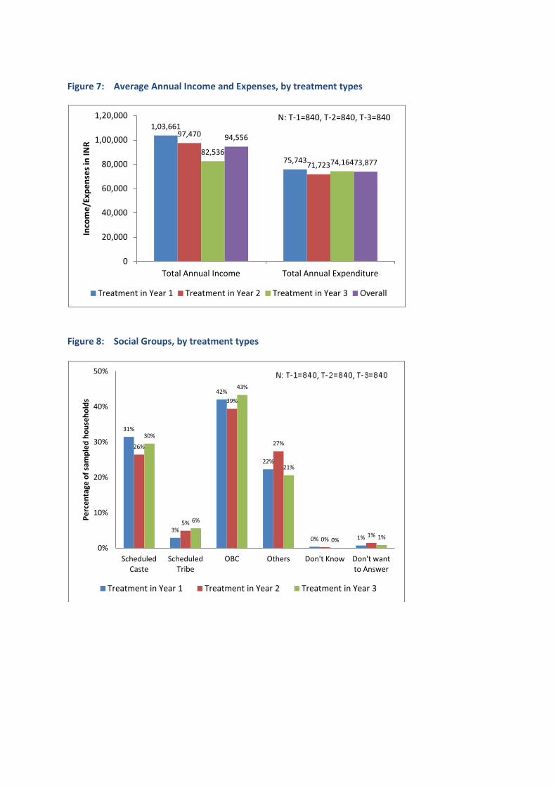
Figure 7: Average Annual Income and Expenses, by treatment types

Figure 8: Social Groups, by treatment types

1,03,661

75,743

97,470

71,723

82,536 74,164

94,556

73,877

0

20,000

40,000

60,000

80,000

1,00,000

1,20,000

Total Annual Income Total Annual Expenditure

Inco

me

/Exp

en

ses

in IN

R

Treatment in Year 1 Treatment in Year 2 Treatment in Year 3 Overall

31%

3%

42%

22%

0% 1%

26%

5%

39%

27%

0% 1%

30%

6%

43%

21%

0% 1%

0%

10%

20%

30%

40%

50%

Scheduled Caste

Scheduled Tribe

OBC Others Don't Know Don't want to Answer

Pe

rce

nta

ge o

f sa

mp

led

ho

use

ho

lds


N: T-1=840, T-2=840, T-3=840

Figure 9: Distribution of Samples on Religion, by treatment types

Figure 10: Gender of head of the household, by treatment types

83%

16%

0% 0% 1%

79%

20%

0% 1% 0%

82%

17%

1% 0% 0%

0%

10%

20%

30%

40%

50%

60%

70%

80%

90%

Hindu Muslim Christian Sikh Others

Pe

rce

nta

ge o

f sa

mp

led

ho

use

ho

lds


91.8%

7.5% 0.6%

0%

10%

20%

30%

40%

50%

60%

70%

80%

90%

100%

Male-headed Household

Female-headed Household

Other

Pe

rce

nt

of

Ho

use

ho

lds


N: T-1=840, T-2=840, T-3=840

N: T-1=840, T-2=840, T-3=840

Figure 11: Type of Housing, by treatment types

The samples start at similar levels of social and occupational status making them comparable.

30%

47%

23%

29%

45%

25% 25%

44%

31%

0%

5%

10%

15%

20%

25%

30%

35%

40%

45%

50%

Pucca House Semi-Pucca House Kutcha House

Pe

rce

nt

of

Ho

use

ho

lds


N: T-1=840, T-2=840, T-3=840

Box 1: Indicators for computing MPI Education (each indicator is weighted equally at 1/6 )

• Years of Schooling: deprived if no household member has completed five years of schooling • Child Enrolment: deprived if any school-aged child is not attending school in years 1 to 8

Health (each indicator is weighted equally at 1/6) • Child Mortality: deprived if any child has died in the family* • Food Security: deprived if the household faced a food shortage at any time during the last year**

Standard of Living (each indicator is weighted equally at 1/18) • Electricity: deprived if the household has no electricity • Drinking water: deprived if the household does not have access to clean drinking water or clean water is more than 30 minutes’ walk from home • Sanitation: deprived if they do not have an improved toilet or if their toilet is shared • Flooring: deprived if the household has dirt, sand or dung floor • Cooking Fuel: deprived if they cook with wood, charcoal or dung • Assets: deprived if the household does not own more than one of: radio, TV, telephone, bike, or motorbike, and do not own a car or tractor

* In order to better capture the impact of the 3-year SIDBI program, the child mortality question was limited to 3 years. The original MPI considers a household deprived if a child under 5 has ever died in the family ** The original MPI uses malnutrition among children. Due to the high time and monetary cost of completing anthropometric surveys, a variety of alternate measures for nutrition were explored. Food security was found to be the most efficient and effective substitute.

4.2 Impact Indicators

Flowing from the evaluation model presented in the methodology section, this section presents the results from the analysis (including linear regressions) of the main impact indicators. The results presented here depict the current status of the three sample groups. The first is treatment in year 1 which receives the Project in year 1 and receives it for all 3 years. The second is treatment in year 2 which receives the project in year 2 and for 2 years. Finally, the third group receives the Project in year 3 for 1 year.

4.2.1 Multidimensional Poverty Index The MPI, which has been developed by the Oxford Poverty and Human Development Initiative, uses 10 indicators (see Box 1) covering three dimensions, namely education, health, and standard of living. Each dimension is weighted equally, with education and health containing two indicators each and standard of living containing six. Unlike standard poverty measures, which tend to look only at headcounts (% of poor), the MPI also examines the acuteness of poverty. Each surveyed household is considered deprived or not at each indicator, with the average deprivations for a poor household representing the extent of poverty. An MPI score is calculated2 by combining the intensity and incidence (%) of poverty in any given area. The MPI ranges from 0 to 1 and a higher level of MPI indicates greater extent of deprivation.

2Alkire and Santos 2010

The MPI and the incidence and intensity of poverty across the project area and treatment types are presented in Figure 12. Figure 12: Multidimensional Poverty Index in its Composite Measures across treatment groups,

2012

As per the results the incidence of multi-dimensional poverty in sample areas is about 75%. It is marginally higher in households receiving treatment in year 2 but the difference is not significant. The intensity of poverty (which denotes the proportion of factors in which the household is poor) is very similar across all three groups. The MPI is highest for the households which receive treatment in Year 2 by 0.02 points. This is not a significant difference and as such the three groups are fairly comparable. The linear regression model, given in Table 5 on the MPI draws the following significant explanatory variables.

Credit from MFIs. This indicates that a larger loan from an MFI is correlated with greater extent of poverty. This may indicate that loans from MFIs are being undertaken to meet immediate consumption and cash needs.

Occupation: Those in labour have a higher degree of poverty than other occupations since the coefficient is significant and positive. Those in agriculture and allied occupations have a higher degree of poverty than other occupations since the coefficient is significant and positive.

Literacy of Head of Household: Households where the head is literate have a lower MPI and thus lesser degree of poverty and deprivation.

Caste: Socially excluded groups and OBCs have a higher MPI than other social groups.

0.74

0.49

0.36

0.77

0.50

0.39

0.74

0.49

0.36

0.75

0.49

0.37

0.00

0.10

0.20

0.30

0.40

0.50

0.60

0.70

0.80

0.90

Incidence of Poverty Intensity of Poverty MPI


N: T-1=840, T-2=840, T-3=840

Table 5. Linear Regression Analysis with Multidimensional Poverty Index as Dependent Variable,

2012

Variables Coefficient Std. Error t-Statistic p-Value

Multidimensional Poverty Index

Socially Excluded Groups 0.0315*** (0.00868) 3.63 0.000

Other Backward Castes -0.00498 (0.00801) -0.62 0.534

Literacy -0.0741*** (0.00638) -11.6 0.000

Distance from Nearest Town -0.000166 (0.000151) -1.1 0.272

Labour 0.0759*** (0.00765) 9.92 0.000

Agriculture and allied Occupation

0.0672*** (0.00847) 7.94 0.000

Institutional Credit 3.09e-07 (2.79e-07) 1.11 0.268

Credit from MFI 3.69e-06*** (4.30e-07) 8.58 0.000

Financial Literacy 0.0153 (0.0167) 0.92 0.359

Constant 0.388*** (0.0120) 32.36 0.000

Observations 2,520

R-squared 0.140

Standard errors in parentheses

*** p<0.01, ** p<0.05, * p<0.1

Box 2: Indicators for computing PPI Indicators used for computing PPI are:

Number of people aged 0 to 17 in the household

Household’s principal occupation

Type of housing

Primary source of energy for cooking for the household

Household owning the following: o a television o a bicycle, scooter, or motor cycle o an almirah/ dressing table o a sewing machine o number of pressure cookers or

pressure pans o number of electric fans

Scores assigned for each of the indicators, with a maximum possible score of 100

4.2.2 Progress out of Poverty Index

The PPI, developed by the Grameen Foundation, uses 10 key indicators (see Box 2) to estimate the likelihood that a household has income below the five levels: (a) $0.75/Day/PPP (purchasing power parity), (b) $1/Day/PPP, (c) $1.25/Day/PPP, (d) $1.50/Day/PPP, and (e) $2/Day/PPP. These indicators are unique to each country and derived from standard national surveys. In addition, the indicators are selected on the basis of being easy and inexpensive to collect, being sensitive to changes in levels of poverty over time, and being strongly correlated with poverty. Driven by poverty data, each indicator is weighted towards a total PPI score, which is on a 0-100 scale. Higher scores indicate less likelihood of poverty. With 90% confidence, estimates of groups' overall poverty rates are accurate to within +/-2 percentage points3. In the case of India, the PPI indicators were derived from the National Sample Survey Organizations 2005 Social-Economic Survey4. For the present impact evaluation, all ten indicators were used as designed.

As shown in Figure 13, the Progress out of Poverty index is marginally higher in the group that receives treatment in year 2. However, there isn't a significant difference between these groups. In all these groups, based on the standard PPI likelihoods, the proportion of households below the national poverty line would be 18%. In addition, 29.7% of the sample households across the three treatment groups are likely to be below the $1/day PPP poverty line.

3http://progressoutofpoverty.org/en/technical-platform 4http://progressoutofpoverty.org/india

http://progressoutofpoverty.org/en/technical-platform

http://progressoutofpoverty.org/india

Figure 13: Progress Out of Poverty Score across Treatment Types, 2012

In this regression model given in Table 6, the following are key significant variables.

Financial literacy: Financial literacy is significant and positive indicating that a higher degree of financial literacy is correlated with higher PPI, and therefore economic well-being.

Institutional credit: Institutional credit has a significant and positive effect on PPI though the coefficient is fairly small.

Caste: Socially excluded groups have a lower PPI than others, with the difference being 4.3 Other backward castes have a lower PPI than others, with the difference being 2.9 points.

Occupation: Those in labour occupations have a lower PPI than other occupations.

30.96 31.15 30.96

0

5

10

15

20

25

30

35


PP

I Sco

re

Progress Out of Poverty Index (PPI) N: T-1=840, T-2=840, T-3=840

Table 6. Linear Regression Analysis with Progress out of Poverty Index as Dependent Variable, 2012


Progress out of Poverty Index

Socially Excluded Groups -4.307*** (0.653) -6.6 0.000

Other Backward Castes -2.920*** (0.603) -4.84 0.000

Literacy 5.546*** (0.480) 11.55 0.000

Distance from Nearest Town 0.0217* (0.0113) 1.92 0.055

Labour -9.174*** (0.576) -15.94 0.000


-0.188 (0.637) -0.29 0.768

Institutional Credit 4.46e-05** (2.10e-05) 2.12 0.034

Credit from MFI -7.32e-05** (3.24e-05) -2.26 0.024

Financial Literacy 2.291* (1.257) 1.82 0.068

Constant 33.14*** (0.902) 36.74 0.000

Observations 2,520

R-squared 0.233


*** p<0.01, ** p<0.05, * p<0.1

4.2.3 Women Empowerment Score The women empowerment score is calculated by scoring each household on a set of 15 questions about the involvement of women in decision making. The score ranges from 0 to 1 with 0 indicating no involvement in decision making and 1 being involvement to a great extent. This includes questions related to credit, health, decisions regarding children, assets and political participation. In the theory of change of the program apart from well-being of the clients and their economic status, improved opportunities for women and positional

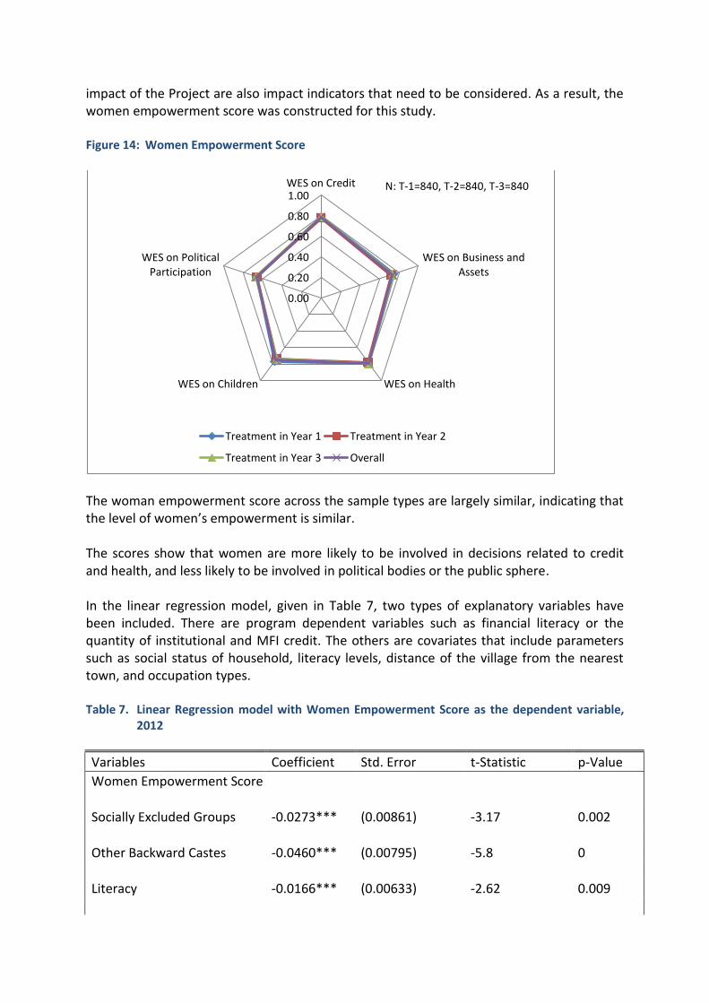
impact of the Project are also impact indicators that need to be considered. As a result, the women empowerment score was constructed for this study. Figure 14: Women Empowerment Score

The woman empowerment score across the sample types are largely similar, indicating that the level of women’s empowerment is similar. The scores show that women are more likely to be involved in decisions related to credit and health, and less likely to be involved in political bodies or the public sphere. In the linear regression model, given in Table 7, two types of explanatory variables have been included. There are program dependent variables such as financial literacy or the quantity of institutional and MFI credit. The others are covariates that include parameters such as social status of household, literacy levels, distance of the village from the nearest town, and occupation types. Table 7. Linear Regression model with Women Empowerment Score as the dependent variable,

2012


Women Empowerment Score


Other Backward Castes -0.0460*** (0.00795) -5.8 0

Literacy -0.0166*** (0.00633) -2.62 0.009

0.00

0.20

0.40

0.60

0.80

1.00 WES on Credit

WES on Business and Assets

WES on Health WES on Children

WES on Political Participation

Treatment in Year 1 Treatment in Year 2

Treatment in Year 3 Overall

N: T-1=840, T-2=840, T-3=840

Distance from Nearest Town -0.000295** (0.000150) -1.97 0.048

Labour -0.00486 (0.00759) -0.64 0.522


0.0375*** (0.00840) 4.47 0

Institutional Credit 5.95e-07** (2.77e-07) 2.15 0.032

Credit from MFI -3.12e-06***

(4.27e-07) -7.31 0.000

Financial Literacy 0.0101 (0.0166) 0.61 0.541

Constant 0.785*** (0.0119) 66.03 0.000

Observations 2,520

R-squared 0.066


*** p<0.01, ** p<0.05, * p<0.1

Significant variables in this model include:

Credit from MFI, the coefficients for which indicate that households with lower women empowerment score are served more by MFIs than other sources.

Institutional credit, suggesting suggest that as institutional credit increases the level of empowerment among women increases. However, the coefficients on these parameters are very low indicating that the quantum of effect is small.

Caste, where socially excluded groups (SC and ST) and other backward castes have a lower level of women empowerment currently than other groups. All else being equal this difference is roughly between 0.027 points and 0.046 points respectively.

Literacy of head of the household: Households where the head of household is illiterate also have a lower women empowerment score.

Occupation: Those working in agriculture and allied occupations (including livestock, poultry and fishery) have a higher gender empowerment score.

From the FGDs the women say that MFIs (and in a few reported cases SHGs) have enabled women to participate in the credit market. It has helped them grow their enterprises and contribute positively to the household income. This has translated into improvement in the status of women within the family, and recognition of this contribution. From an FGD in Chhindwara, MP the women feel that “Due to MFIs women make groups and help each other. They understand the importance of education. Today women help in the financial

needs of her family and social attitudes are changing. Now we participate in decision taking in the family”. Women participate to a large extent in decisions relating to health, education and marriage of children. However men take decisions related to land purchase and other decisions related to livelihoods. Women also do not have any say in political decision making. With respect to financial matters in most FGDs the women say that the men take decisions – on where to take loans from, how much to take, how to utilize it. From FGDs in Satna and Sagar, MP, the women say are consulted in this regard, but the final decision is left to the men. From one FGD in Allahabad, UP the women admit that even though they apply for the loan and get it in their name, the men in the family are engaged in the business.

4.3 Outcome Indicators

4.3.1 Household Income and Expenditure The first outcome indicators included in the analysis are household income and expenditure. Annual income refers to income accruing to a household in one year from all employment sources. Total expenditure is the total amount of money spent by the house on various requirements and products for one year. The results of the regression and descriptive analysis are presented below.

Household Income Linear Regression on Household Income A linear regression, as given in Table 8 was conducted using annual household income as dependent variable to assess what factors affect household income at baseline. Table 8. Linear Regression Analysis on Annual Household Income from Sample Households, 2012


Annual Household Income

Socially Excluded Groups -25,904*** (5,988) -4.33 0.000

Other Backward Castes -14,271*** (5,529) -2.58 0.010

Literacy 7,362* (4,406) 1.67 0.095

Distance from Nearest Town 235.0** (104.1) 2.26 0.024

Labour -33,881*** (5,281) -6.42 0.000


19,904*** (5,844) 3.41 0.001

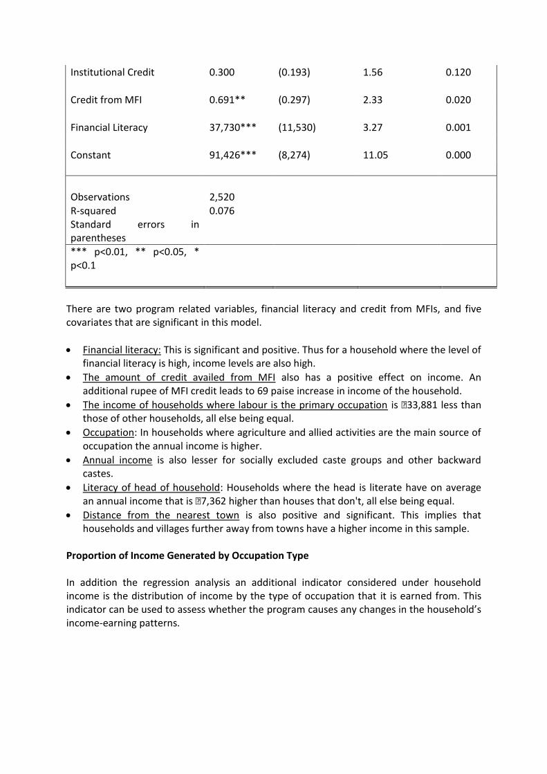
Institutional Credit 0.300 (0.193) 1.56 0.120

Credit from MFI 0.691** (0.297) 2.33 0.020

Financial Literacy 37,730*** (11,530) 3.27 0.001

Constant 91,426*** (8,274) 11.05 0.000

Observations 2,520

R-squared 0.076


*** p<0.01, ** p<0.05, * p<0.1

There are two program related variables, financial literacy and credit from MFIs, and five covariates that are significant in this model.

Financial literacy: This is significant and positive. Thus for a household where the level of financial literacy is high, income levels are also high.

The amount of credit availed from MFI also has a positive effect on income. An additional rupee of MFI credit leads to 69 paise increase in income of the household.

The income of households where labour is the primary occupation is ₹33,881 less than those of other households, all else being equal.

Occupation: In households where agriculture and allied activities are the main source of occupation the annual income is higher.

Annual income is also lesser for socially excluded caste groups and other backward castes.

Literacy of head of household: Households where the head is literate have on average an annual income that is ₹7,362 higher than houses that don't, all else being equal.

Distance from the nearest town is also positive and significant. This implies that households and villages further away from towns have a higher income in this sample.

Proportion of Income Generated by Occupation Type In addition the regression analysis an additional indicator considered under household income is the distribution of income by the type of occupation that it is earned from. This indicator can be used to assess whether the program causes any changes in the household’s income-earning patterns.

Figure 15: Proportion of Household Income earned from various occupation types across

treatment groups, 2012

Figure 15 shows that most of the income earned by the households falls under the category of “Other occupations” and the enterprise based income is less. About 20% of the income is earned from agriculture and allied enterprises as well as from non-agricultural enterprises. Household Expenditure Another outcome indicator used in the analysis is household expenditure because it can be a proxy for income. The amount of expenditure and the item it is made on can indicate changes in economic well-being of the household. For example, increased spending on education and other productive purposes can be considered as a sign of positive impact if attributable to the program.

20%

26%

25%

24%

20%

21%

22%

21%

60%

53%

53%

55%

0% 10% 20% 30% 40% 50% 60% 70% 80% 90% 100%

Treatment in Year 1

Treatment in Year 2

Treatment in Year 3

Overall

Occupation Type as a Percentage of Total Income

Income from Agricultural and Allied Enterprises

Income from Non-Agricultural Enterprises

Other Occupations N: T-1=840, T-2=840, T-3=840

Annual household Expenditure Pattern Figure 16 depicts the average annual household expenditure by treatment type. The graph shows the quantum of expenses being made under each head. The average annual expenditure across the three treatment groups is fairly similar and in the range of ₹71,723 to ₹75,742 a year. Close to 50% of this expenditure annually goes towards food and provisions. In the other categories utilities (such as electricity, water and cooking fuel), travel expenses and expenditure of clothing are the highest ranging between ₹5,000 to ₹7,000. Figure 16: Average Annual Household Expenditure in Sample Households in INR, (2012)

Table 9. Linear Regression Analysis on Household Expenditure, 2012


Annual Expenditure


Other Backward Castes -4,923 (3,869) -1.27 0.203

Literacy 285.4 (3,083) 0.09 0.926

Distance from Nearest Town 184.8** (72.86) 2.54 0.011

0

10,000

20,000

30,000

40,000

50,000

60,000

70,000

80,000


Ho

use

ho

ld E

xpe

nse

s in

INR

Food and Provisions House Rent Utilities

Communications Travel Expenses Liquor/Smoking/Entertainment

Clothes, Footwear, Haircut Festivals/Functions Education Related

Insurance Premiums Loan Repayments Health Related

Home Improvement Other N: T-1=840, T-2=840, T-3=840

Labour -21,967*** (3,696) -5.94 0.000


-7,113* (4,090) -1.74 0.082

Institutional Credit 0.486*** (0.135) 3.6 0.000

Credit from MFI 0.552*** (0.208) 2.66 0.008

Financial Literacy 28,962*** (8,069) 3.59 0.000

Constant 73,519*** (5,791) 12.7 0.000

Observations 2,520

R-squared 0.048


*** p<0.01, ** p<0.05, * p<0.1

In the linear regression model as shown in Table 9 significant variables include:

Financial literacy, credit from MFIs and credit from institutional sources have coefficients that are significant and positive. This indicates that expenditure increases as borrowings from these sources and financial literacy increases.

Occupation: Expenditure is lesser for households where the primary occupation is labour or agriculture.

Distance from town: For each kilometer of distance a village is from the nearest town the expenditure of the household increases by ₹184. Thus, here being further away from town has a positive effect on expenditure.

Average annual income and expenses The average amount of income and expenses across treatment groups are taken as a proxy for economic status of the household.

Figure 17: Average annual income and expenditure

The Treatment in Year 1 sample households have on average a higher income level relative to expenses when compared to the other two treatment groups. The expenses level for all three treatment groups is similar.

4.3.2 Enterprises The objective of the project is to provide financial inclusion to underserved areas by focusing on responsible microfinance. The expectation is that availability of credit would encourage its use in productive purposes, such as enterprises, that in turn generate income for the household and thus benefit them economically. Thus, income generated from enterprises is another outcome indicator included in the analysis.

Table 10. Linear Regression on Annual Income Earned from Enterprises, 2012




Other Backward Castes -6,990** (2,729) -2.56 0.010

Literacy 2,187 (2,175) 1.01 0.315

Distance from Nearest Town 156.4*** (51.39) 3.04 0.002

Labour -47,238*** (2,607) -18.12 0.000


-45,551*** (2,884) -15.79 0.000

1,03,661

75,743

97,470

71,723

82,536

74,164

94,556

73,877

0

20,000

40,000

60,000

80,000

1,00,000

1,20,000

Total Annual Income Total Annual Expenditure

Inco

me

/Exp

en

ses

in IN

R


N: T-1=840, T-2=840, T-3=840


Credit from MFI 0.795*** (0.147) 5.42 0.000

Financial Literacy 6,063 (5,691) 1.07 0.287

Constant 51,294*** (4,084) 12.56 0.000

Observations 2,520

R-squared 0.181


*** p<0.01, ** p<0.05, * p<0.1

The significant covariates in this model as shown in Table 10 are as follows:

Credit from MFIs is significant and positive. The coefficient indicates that a ₹1 increase in borrowings from an MFI results in a 79 paise increase in income from non-agricultural enterprise.

Occupation: Households where labour and agriculture are primary occupations have less income from these enterprises.

Caste: Socially excluded caste groups and other backward castes also have lesser income compared to others, with the difference being ₹12,024 and ₹6,990 on average respectively, all else being equal.

Distance from town is also significant. For every kilometer increase in distance, income increases by ₹156.

Enterprise Ownership In addition to the regression analysis another indicator of change would be the proportion of the sample that owns an enterprise. Figure 18 depicts the enterprise ownership levels in the sample.

Figure 18: Proportion of Sample Households owning a business, 2012

The highest proportion of enterprise ownership is in the group which receives treatment in year 3 while it is least for the first year. About two-thirds of the entire sample doesn’t own any enterprises.

4.4 Financial Indicators

The main aim of the Project is to deliver microfinance products to underserved areas and to also address the gaps in the quality of microfinance service by focusing on responsible microfinance. Thus indicators on the status of financial literacy, access and utilization of credit (and its purposes), as well as access and utilization of other financial products such as savings and insurance were included in the analytic model. In this section the baseline status on these indicators is presented.

4.4.1 Financial Literacy Financial literacy refers to knowledge of financial products and practice and here it is measured by using a financial literacy score. The financial literacy score is calculated by taking the average of responses on various questions on awareness about interest rates, credit, savings and insurance sources, and knowledge and practice related to budgeting and savings. The responses are coded as 0 for unplanned and irregular behaviour and as 1 for planned and regular behaviour. Some of the responses on awareness are coded as proportion of total possible sources of which the respondent has knowledge. Based on this, a final financial literacy score is calculated on a scale of 0 to 1, with 1 being highest possible level of financial literacy and 0 being the least. Figure 19 depicts the average financial literacy score across the treatment groups.

32.86%

35.95%

39.40%

36.07%

10%

15%

20%

25%

30%

35%

40%

45%

50%


Pe

rce

nt

of

Ho

use

ho

lds

N: T-1=840, T-2=840, T-3=840

Figure 19: Financial Literacy Score for Sample Households, 2012

In this case, current financial literacy levels in the three treatment groups are comparable. The numbers suggest that on average respondents are aware of or exhibit 44% of good practices and sources for credit and savings. The standard deviation for financial score is about 0.19 in all of the groups. This suggests that 67% of the respondents have a financial literacy score between 0.62 and 0.24.

4.4.2 Savings

There are multiple products and services offered by micro finance institutions, including savings that need to be considered here. This section discusses some key indicators related to savings practices. Households availing savings The first indicator included here is the percentage of households actually availing savings. Figure 20 depicts these results. Savings in the group that receives the treatment in year 1, at 68.9% is the least, compared to the groups which receive it in year 2 and 3, for which it is 77.3% and 74.8% respectively. Thus in terms of savings there is difference in starting points of the 3 groups. These savings may be made at home or some other informal source (for example with friends/relatives) or they may be in formal institutions such as banks, post office etc.

0.44

0.42

0.44 0.43

0.35

0.37

0.39

0.41

0.43

0.45

0.47

0.49


Fin

anac

ial L

ite

racy

Sco

re

N: T-1=840, T-2=840, T-3=840

Figure 20: Percent of households that have availed savings, 2012

Source of Savings Part of the goal of the project, by providing responsible microfinance, is to reduce the dependence on informal sources of borrowing and lending. Thus the distribution of the savings of a household across various sources is depicted in Figure 21. Figure 21: Average Percent of savings in each type of source by sample households. 2012

The type of sources used for savings are fairly similar across the treatment groups currently. Formal sources such as banks and SHGs are used most frequently. Among the informal

69%

77%

75% 74%

50%

55%

60%

65%

70%

75%

80%

Treatment in Year 1

Treatment in Year 2

Treatment in Year 3

Overall

Pe

rce

nt

of

Ho

use

ho

lds

3%

83%

37%

5%

79%

38%

2%

83%

31%

3%

82%

35%

0%

10%

20%

30%

40%

50%

60%

70%

80%

90%

MFI Formal Sources Informal Sources

Pe

rce

nt

of

Ho

use

ho

lds

that

Sav

e


N=T1: 579, T2: 649,T3: 628

N: T-1=840, T-2=840, T-3=840

sources, savings at home are the most common. Only about 2 to 3% of households use MFIs for the purpose of savings.

4.4.3 Credit Access to Credit The first indicator for results on access to credit is the number of loans outstanding for the sample household. This gives an indication of the amount of credit accessed in the sample households. Figure 22 depicts the percentage of sample households that currently have 0, 1, 2 or 3 outstanding loans. Figure 22: Percentage of Sample Households having outstanding loans, 2012

Figure 22 shows that the results in the three treatment groups for this sample are roughly similar. A majority of the sample households do not have any outstanding loans (ranging from 64% to 69%). The rest of the households have 1 outstanding loan and a few respondents, a few households in all three groups have 2 outstanding loans. For outstanding loans the type of source accessed is also analyzed as an indication of the degree of penetration of various sources in the study area. Figure 23 depicts the percent of households that are accessing loans from the following three types of sources: MFIs, Formal sources and informal sources.

67.02% 64.88% 68.93% 66.94%

30.48% 33.33% 28.10% 30.63%

0%

10%

20%

30%

40%

50%

60%

70%

80%

90%

100%

Treatment in Year 1

Treatment in Year 2

Treatment in Year 3

Total

Pe

rce

nt

of

Ho

use

ho

lds

None One Two Three

N: T-1=840, T-2=840, T-3=840

Figure 23: Percent of Households with availed loans in each of the following sources. 2012

In the study area MFIs are the most commonly accessed source for loans with about 20% of households in each of the treatment areas accessing loans from MFIs. On the other hand formal sources (such as nationalized banks and cooperatives) as well as informal sources (such as friends, relatives, money lenders and pawn-brokers) are not accessed as often for the purpose of availing credit. The distribution of the three types of sources is similar across all three groups. In addition the total number of sources from which current loans are accessed is also considered and the results are presented in Figure 24. Figure 24: Number of sources for credit accessed by sample households. 2012

18.9%

23.7%

19.0% 20.6%

9.2%

4.9% 6.8% 6.9%

5.7% 7.3%

6.0% 6.3%

0%

5%

10%

15%

20%

25%

Treatment in Year 1

Treatment in Year 2

Treatment in Year 3

Overall

Pe

rce

nt

of

Ho

use

ho

lds

MFI Formal Informal

67.38% 65.00% 68.93% 67.10%

30.83% 33.69% 29.29% 31.27%

1.19% 1.19% 1.55% 1.31%

0%

10%

20%

30%

40%

50%

60%

70%

80%

90%

100%

Treatment in Year 1

Treatment in Year 2

Treatment in Year 3

Overall

Pe

rce

nt

of

Ho

use

ho

lds

0 Sources 1 Source 2 Sources 3 Sources

N: T-1=840, T-2=840, T-3=840

N: T-1=840, T-2=840, T-3=840

A majority of the respondents in all three groups reported that they have not accessed any loans. This indicates that the penetration of credit is low in these areas and they are possibly underserved. About 30% to 33% of the respondents across the three groups have availed loans from one source. Only about 1% to 1.5% of all respondents have accessed loans from 2 sources and a negligible number of total respondents have accessed loans from 3 sources. Types of sources for availed loans by Social Status, Religion and PPI The type of sources of credit one has access to can be affected by the social or economic profile of the household. To test this in this section results are also presented on the distribution of the various types of sources across the sample households by social status, religion and Progress out of Poverty Index of the household. Figures 25 and 26 and Table 11 present the results by social status, religion and table by PPI respectively. Figure 25: Percent of households availing loans from each type of Source by Social Category. 2012

In the “other group” there isn’t much difference between access to various types of sources accessed, with 9% of the households having availed loan(s) from formal sources. On the other hand the other three groups – Schedule Caste, Schedule Tribe and OBC households are much more dependent on MFI sources for access to loans. Among ST households, dependence on informal sources for loans is the highest at 11%.

17%

25% 27%

12%

7% 5% 6%

9%

6%

11%

7% 5%

0%

5%

10%

15%

20%

25%

30%

Schedule Caste Schedule Tribe OBC Others

Pe

rce

nt

of

Ho

use

ho

lds

MFI Formal Informal

N: SC=734, ST=112, OBC=1048, Other: 590

Figure 26: Percent of households availing loans from each type of source by religion. 2012

The proportion of Sikhs and Others in the sample is limited. Of the rest of the population, Muslim households are more dependent on credit from MFIs (30% of households) as opposed to Hindu (19%) and Christian (20%) of the households. Table 11. Average PPI of households by loan source availed

Average PPI of those availing loans

Average PPI for those not availing loans

N

Availing Not-Availing

MFI 28.47 31.60 518 2002

Formal 33.79 30.75 175 2345

Informal 27.16 31.21 159 2361

The average PPI of households availing MFI and informal loans is lower than that of households availing loans from formal sources. The difference in average isn’t very vast, however, it does indicate that those with a lower economic status tend to opt for informal loans more. Average size of Outstanding and Repaid Loans by source Apart from the proportion of households that have availed loans, the size of the loan and the contribution of the different type of sources to it is also an important outcome indicators. It is expected that by going to underserved areas MFIs will reduce dependence on informal sources and borrowing from MFIs and other formal sources will increase. Figure 27 presents the results.

19%

30%

20%

9%

0%

8%

3%

10%

0%

23%

6% 8%

0%

9%

0% 0%

5%

10%

15%

20%

25%

30%

35%


MFI Formal Informal

N: Hindu= 2041, Muslim=443, Christian=10, Sikh: 11, Other: 13

Figure 27: Average Size of Outstanding loan (in INR), 2012

The loan size for loans from formal sources is much larger compared to others. The loans availed from MFIs are much smaller in size. The results are similar for the repaid loans, where across treatment groups the formal and informal sources have much larger loan sizes compared to the MFIs on average for the household. Figure 28 depicts these results.

Figure 28: Average size of repaid loans by treatment type, 2012

28,825 29,841 30,175 29,503

15,226 15,198 16,134 15,496

27,729 19,508

22,110 22,808

-

10,000

20,000

30,000

40,000

50,000

60,000

70,000

80,000

Treatment in Year 1

Treatment in Year 2

Treatment in Year 3

Overall

Ave

rage

siz

e o

f o

uts

ten

din

g lo

an a

mo

un

t in

IN

R

Formal Sources MFIs Informal Sources

16,331 22,104 21,758 19,764

14,908 14,800 16,673

15,492

19,645 17,121

24,098 20,531

0

10,000

20,000

30,000

40,000

50,000

60,000

70,000

Treatment in Year 1 Treatment in Year 2 Treatment in Year 3 Overall Ave

rage

siz

e o

f re

pai

d lo

an a

mo

un

t in

INR

Average Size of Loans from Formal Sources

Average Size of Loans from MFI

Average Size of Loans from Informal Sources

N: Formal= 175, MFI=518, Informal = 159

N: Formal= 184, MFI=361, Informal = 112

Cost of credit

Weighted Average Cost of Credit

N

Treatment in Year 1 15% 270 Treatment in Year 2 14% 277 Treatment in Year 3 15% 248

Overall 15% 795 The weighted average cost of credit is 15% and similar across all treatment types. The average cost of credit is further analyzed by the type of source and the results are below in Table 12 Table 12. Weighted average cost of credit by Source from which loan is availed. 2012

Treatment in Year

1

Treatment in

Year 2

Treatment in Year

3 Overall

Formal 9% 8% 11% 9%

MFI 14% 14% 16% 15%

Informal 29% 18% 21% 22%

Friends/Relatives 19% 12% 13% 14%

N 270 277 248 795

The above table depicts the weighted average cost of credit for each of the three treatment types in the sample by the source of the loan. The cost of credit here is the average interest rate charged on the loan per annum weighed by the size of the loan. The highest cost of credit is for those availing loans from informal sources with the highest being an average of 29% per annum in the Treatment in Year 1 group. The interest rate is least for those availing loans from formal institutions such as banks and cooperatives at 9% to 11% across the three treatment groups. Figure 29 also depicts the distribution of the various sources across the ranges of the weighted average cost of credit.

Figure 29: Percent of total number of loans availed from various sources by ranges of weighted

average cost of credit, 2012

Figure 29 shows the distribution of the loans across various ranges of weighted average interest rates (less than 10%, 10 to 20% etc.) and across the four different types of sources from which credit is available. A majority of the loans from formal sources and a majority of the loans from friends, neighbours and relatives have interest rates that are less than 10% per annum. On the other hand for MFIs 62% of the loans fall into the 10% to 20% range. For the informal sources there is more variation in the results with 32% of the loans falling in the less than 10% range, 27% of the loans falling in the 10 to 20% range and 22% falling in the 30% to 40% range. The results indicate that a majority of the loans from formal sources and from friends/relatives/neighbours fall into lower brackets of cost of credit and are thus generally less expensive when compared to the loans from MFIs and informal sources. The latter have a higher percentage of loans falling into the larger cost of credit brackets.. Purpose of the Loan The goal of the responsible microfinance program is to ultimately impact standard of living through improved access to credit. By targeting credit constraints it is expected that the households will use the credit and invest it in productive purposes which will in turn lead to an improved economic status for the household. Figure 30 represents the results. Figure 30: Purpose of loans taken as a percentage of the households availing loans. 2012.

58%

75%

33% 32%

12%

21%

62%

27%

16%

2% 4%

22%

8% 2% 1%

17%

0%

10%

20%

30%

40%

50%

60%

70%

80%

90%

100%

Friends/Relatives/ Neighbours

Formal MFI Informal

Pe

rce

nt

of

Loan

s A

vaile

d

Less than 10% 10% to 20% 20% to 30% 30% to 40% More than 40%

N: Friends/Relatives/Neighbours = 100, Formal= 175, MFI=518, Informal = 59

The patterns are largely similar across the three treatment groups. The highest percentage of loans is availed by households for starting a new business (24% to 26%) or for acquiring assets for a new business (22% to 36% households). In the group that receives treatment in year 3 the percent using credit for the purchase of new assets is slightly higher than others at 36%. Thus, currently most of the loans are being utilized for business purpose. However, the overall level of access to credit is still low. Apart from business purposes loans are also availed to purchase household assets and to resolve cashflow problems in the household most frequently (at 10 to 14% n the various treatment groups). Terms and Conditions associated with Credit In this section the terms and conditions associated with outstanding loans such as repayment schedule and additional charges are analyzed. The first indicator under terms and conditions, as given in Table 13 is additional charges levied for availing loans. Table 13. Additional charges levied for availing loans in INR

Treatment in Year 1

Treatment in Year 2

Treatment in Year 3 Overall

Formal 7.51 7.02 6.93 7.21

Friends/Relatives/Neighbours 11.39 16.74 4.29 11.49

Informal 12.00 9.22 4.26 8.31

MFI 6.85 5.71 5.86 6.10

N 300 308 289 897

The additional charges are calculated as an average per loan within each of the listed source category. The highest additional average charges were in the informal sources and friends, relatives and neighbours category at about ₹9 to ₹12 rupees per loan. There is a lot of variation across the three treatment groups with Treatment in year 3 having average charges for formal sources of ₹6.93. Given the small numbers within each group and the marginal differences it is unlikely that these differences significant.

26% 22%

13%

8% 12%

4% 1%

8%

12%

24%

29%

10%

4%

17%

2% 2%

7% 10%

24%

36%

10% 7%

14%

2% 3% 6%

9%

0% 5%

10% 15% 20% 25% 30% 35% 40%

Star

t a

Bu

sin

ess

New

Ass

ets

for

bu

sin

ess

New

Ho

use

ho

ld

Ass

ets

Cas

hfl

ow

in b

usi

nes

s

Cas

hfl

ow

in

ho

use

ho

ld

Rep

ay o

ld

loan

s/in

tere

sts

Ch

ildre

n's

Ed

uca

tio

n

Hea

lth

Exp

ense

s

Oth

er

Pe

rce

nt

of

Ho

use

ho

lds

avai

ling

loan

s


N: T-1= 274, T-2=288, T-3 = 259

The second indicator is duration of the loan as shown in Figure 31 Figure 31: Duration of loan availed as a percent of total loans, 2012

The patterns are very similar across the three treatment groups. A majority of the loans (55% to 60%) have a duration of 6 to 12 months. The next most common duration is 1 to 2 years, followed by more than 2 years (8% to 14%). The third indicator is the repayment schedule, as shown in Figure 32. Figure 32: Type of repayment schedule for loan availed as a percent of total loans availed, 2012

58% 60% 55% 58%

18% 19%

15% 17%

14% 8% 13% 12% 4% 4% 5% 4%

0%

20%

40%

60%

80%

100%

Treatment in Year 1

Treatment in Year 2

Treatment in Year 3

Overall

Pe

rce

nt

of

Loan

s av

aile

d

Less than 3 Months 3 to 6 Months 6 to 12 Months

1 to 2 years More than 2 Years Don't Know

Other

51.0% 55.8% 52.4% 53.1%

6.3% 6.1% 6.5% 6.3%

16.7% 12.8% 14.7% 14.7%

2.3% 1.0% 1.0% 1.4%

9.0% 8.3% 5.5% 7.6%

9.3% 11.9% 13.0% 11.4%

0%

10%

20%

30%

40%

50%

60%

70%

80%

90%

100%

Treatment in Year 1

Treatment in Year 2

Treatment in Year 3

Overall

Pe

rce

nt

of

Loan

s A

vaile

d

Daily Weekly Fortnightly

Monthly Quarterly Half-Yearly

Annually No Specific Schedule Don't Know

N: T-1= 300, T-2=308, T-3 = 289

N: T-1= 300, T-2=308, T-3 = 289

The patters on repayment schedule are similar across all the treatment groups with weekly repayments being the most common type of schedule. This is followed by monthly repayments (12.8% to 16.7% of the loans). Daily and quarterly repayment schedules are the least common. The current repayment status of availed credit is the fourth outcome indicator, as presented in Figure 33. Figure 33: Repayment status of availed loans as a percent of total number of loans availed. 2012.

Satisfaction with Credit To assess the effectiveness of the delivery of “responsible” microfinance the households were asked certain questions regarding their experience and satisfaction with financial services and products available. A satisfaction score was generated through a set of questions ranging from flexibility, understanding of terms to interest rates. Figure 34 depicts the results for satisfaction score across the three types of sources available.

21.1% 20.0% 16.3% 19.2%

13.6% 8.2% 8.7% 10.1%

52.4% 59.7% 59.7% 57.3%

8.8% 9.2% 12.2% 10.0%

0%

20%

40%

60%

80%

100%


Pe

rce

nt

of

Loan

s A

vaile

d

Regularly Paid and no Dues Regularly paid and 1-2 dues pending

Paying, more than 1-2 dues Irregular and occasional payment

Stopped Repaying Don't Know

Other N: T-1= 300, T-2=308, T-3= 289

Figure 34: Satisfaction with Credit services and products, 2012

The results show that there are higher satisfaction scores from formal sources of loans in comparison to MFI followed by informal sources. MFI scores higher on access and collateral and add on services but low on flexibility and credit limit. The FGDs provide a greater insight on credit needs, sources and satisfaction levels. Participants across all the FGDs, irrespective of state or location expressed three main needs for credit: (a) For enterprise (agriculture, non-land based) for those households who have enterprise; (b) to tide over emergencies, mostly health related; (c) to fulfill social obligations like marriage and death. Informal sources FGD participants from MP and Maharashtra share that they go to friends, relatives, neighbours to tide over small value and short-term credit needs to fulfill some extra household expenses that they may have, or to over tide needs for minor health issues. This source is preferred for short-term needs mainly because it is easily accessible, interest free and there is no fixed or stringent repayment conditions, through the loan is repaid. Participants from Maharashtra stress “friends and family can be approached at any time and they know us well and are able to understand our situation and need for funds.” From one FGD in Latur, Maharashtra the participants have shared that these sources are used for needs up to ₹5,000. However participants from UP don’t prefer to take loans from friends and family, even if small and short-term in nature because they fear being shamed if the friends or family members refuse, or if they are not able to return the money on time. In UP the participants shared that they also receive grocery items on credit from grocery stores, which helps them tide out short-term cash requirements.

0 0.1 0.2 0.3 0.4 0.5 0.6 0.7 0.8 0.9

1 Access to Credit Services

Processing

Collateral

Interest Rate

Flexibility of Repayment Options

Credit Limit

Terms and Conditions

Add On Services

Formal Informal MFI

N: Formal= 1303, MFI=1697, Informal= 658

With larger or emergency fund needs money lenders, pawn brokers, landlords or contractors are approached. Such needs include requiring funds to meet social obligations like weddings and funerals; funds to get healthcare for serious or critical illnesses; funds for land purchase or construction; funds for enterprise. People know that these sources can be exploitative, charging rates as high as 10 percent per month. Pawn brokers take jewellery or assets as surety and there is a risk of these being forfeited in case loans are not repaid on time. Yet these sources thrive since they are easily accessible, they provide large amounts such as ₹10,000-50,000, and the processes to avail the loan are easy. The time period for repayment also tend to be flexible. There is an indication of debt traps, where families are compelled to take loans to repay loans taken earlier. Formal sources The FGD participants do not take credit from formal sources such as banks. Banks “exclude people based on their profile” feel some FGD participants. In effect this means that only people who can pledge assets with significant value like gold and land, and have better repayment capacity can get loans from the banks. Banks also require a lot of documentation which the poor people lack. Except one participant from Satna in MP, all others say that only the rich can get loans from banks. Some feel that are economically too weak to save money in banks and a few that have bank accounts save irregularly. There was one experience from UP where a participant recalled having applied for a loan of ₹10,000 from a bank, and had to pay ₹3,000 to the manager and a middle man to get the loan sanctioned. SHG as a source of credit is reported from few groups in MP and UP. Agriculture and other enterprises and household needs are taken care through credit from SHGs. SHGs are seen as a desirable source since the loans are easily available and the interest is very low and it is seen as the “most considerate source”. However it is not among the top preferred or used sources of credit since the value of loans available from SHG is often inadequate and in some villages women share that some SHGs were a good source of credit but are no longer functional. MFI as a credit source In MP the presence of MFIs is strong with multiple MFIs operating in the villages and towns. All MP FGDs the participants were aware of MFIs operating within their locality, with some having accessed credit through this source. In UP from two villages FGDs participants reported that there is no MFI in the area, and even in Maharashtra the MFI reach in area covered appears to be weak. MFI loans are usually taken for enterprise purpose – petty shops, bangle work, agriculture inputs, poultry and goat enterprises, furniture making, tailoring, bamboo craft, etc. However, there have been few reports of loans being used for other purposes also such as house construction, household consumption, weddings as reported by women in Betul, MP and in Allhabad, UP.

People who have taken loans from MFI have found the ease of access of the loan useful. There is someone from the company who explains the procedure for loan application and also gives them details about the interest and other services (insurance). They are supported in forming groups, and on provision of identity proof they can secure the loan. Many participants find the weekly payment easy to make. Some are particular about repayment and happy that the group puts pressure on individual members who may default, and sometime the group also pays for defaulters, collecting the money from them afterwards. In MP Betul some FGD participants feel that “MFI is the best as we get loan for agriculture during the season to purchase seeds and fertilizers.” In Chhindwara, MP some participants feel that “due to the MFI loan their lifestyles have improved, as the loan has helped them grow their enterprise and increase their incomes.” There are also reports of MFI providing add on services like awareness on social protection schemes, and in one FGD participants also spoke of business services provided to them. The downside of the MFI loan is that the loan amount is not always adequate to meet the credit requirements and people are still compelled to go to pawn brokers and money lenders. The MFI repayment schedule is also very inflexible and the frustration with this was apparent as one FGD participant from Betul, MP complained that “even if you are ill or dying you have to repay the installments at the fixed time and also be physically present otherwise you are penalized from the company.” Such stringent terms and condition not only cause problems for those accessing MFI credit, but is citied by some as reason not to join MFIs. Such perceptions of borrowers show that they don’t fully grasp the reasoning behind such processes that group meeting are a form of surety for the MFI, which otherwise is not insisting on other forms of surety like jewellery, land or other assets; and they are also an opportunity for the group to share and learn. From one town in Chhindwara, MP, the women, all whom have enterprises complain that the MFI needs them to submit documents every time they take a loan, even though they have been linked to the MFI for the past 3-4 years and have always repaid the loan on time. They perceive this as MFI’s not trusting them. They therefore prefer to take credit from the pawn broker, who they say is the second largest source for credit after family and friends. Another issue with MFI credit that participants from Betul and Chinndwara expressed was what they perceived was “cheating” by one of the MFIs. They believe that the MFI charged them two extra installments. While the emotions in such situations run high, these instances have to be considered in the light of the financial literacy of beneficiaries, which shows that perceptions do not match reality. Most of the people in the all the FGDs who had availed loans from MFIs seem to be clear only about the amounts and the corresponding payment schedules – in terms of how much is repaid periodically (weekly in most cases), and within what period (50-55 weeks in most cases). They are able to share the process of getting and repaying the loans. Some of those who have availed loans say that they have been told how the interest is calculated, some say that they were told how the interest is calculated, but don’t remember it. On deeper inspection it appears that most people know very little about the loan product and its components. There is no understanding of flat rates against declining balance rates. There is little clarity on service and other fees being charged. For instance, from most of the

MP FGDs the participants shared that they received accidental insurance as a part of the loan, however they don’t know much more other that they will receive some amount in the event of death of the borrower and the entire loan will be waived and the repaid amount returned to the family. From Chhindwara in MP a group shares how they have not received the weekly amount paid towards insurance at the end of the loan period. In another FGD the participants know that there is an accidental insurance linked to the loan, however they don’t know much about this, except that two people had died but their families have not received the insurance because the paperwork has not come through. Only from one FGD have participants spoken of declining balance of loan being taken. “The official of this company told us that our loan repayments is in decreasing order which will completes in 23 installments. He said we have to deposit 680 rupees on getting ₹12,000 of loan. Then we understood that we have to deposit 21 installments, but in the end we were forced to pay 23 installments. When we argued, demanding to know the reason for this they showed us a court notice and also complained to other MFIs so that they refused us to give loans. ₹60 has been cut by the MFI every month for getting insurance services but they didn’t return this amount till the end of the year. On every ₹12,000 of loan they charged ₹1,050 extra in a wrong manner. They have also charged 1% as loan fees on every loan amount. In this way they cheated us.” This discussion with the group clearly points to a misunderstanding between what is being productized and what is being perceived. The MFI is being transparent – charging interest on declining balance, and providing clarity on all other costs such as fees and insurance. While the groups are aware of the components, the problem lies in its interpretation. In addition, in some cases the reasoning behind certain processes like weekly participation in meetings does not seem to be transferred to the groups for them to appreciate the need for such processes. In terms of grievance redressal, there is very little knowledge of where and how members can lodge complaints. From Dhar, MP one group shares that they know only the MFI staff working in their local office and when they asked about contacts of others senior staff they were told “there is no need for you to know”. In Satna, MP participants felt they could approach the Ward Councilor, district Collector and Sarpanch in case of complaints. Some participants have contacts of the state offices. For those women who have not availed MFI services the reasons are mainly that they are not confident of getting enough income on a weekly basis to make the weekly installment payments. A few also say that their husbands do not want them to join the MFI. Financial inclusion Financial inclusion is poor. Most people don’t have a bank account since they feel that banks are out of the reach of poor people. Even those who have bank accounts say that the savings is irregular and it is not a proffered credit source since the amounts are small and they don’t have the documentation required to get the loans. In UP people know about insurance. Some have life insurance, but most can’t afford it. In one village in Allahabad there is an agent in the village who helps them to open a Recurring

Deposit account in the Post Office. Most of the family are having a RD account in the post office and they depositing ₹50 per month. There is an LIC agent in their village and he has spread awareness on LIC insurance facilities. Some family have taken LIC Insurance policies and some people are also depositing some money in SAHARA as savings. Unmet needs Most FGD participants have not specified unmet needs for credit. They say that when there is emergency they end up taking loans from informal sources, which is available at any time of the day. From one FGD in MP the women share that even after taking loans there are needs which are unmet, like children’s higher education, wedding expenses, etc. They go without these needs.

4.4.4 Investment in Enterprise The intent of the Project, in providing financial services, is to encourage investment in enterprises and other productive endeavours such as education. Thus, one of the outcome indicators examined is the nature and quantum of investment being made into enterprises by the sample households. In this section, the quantity of investment being made into enterprise and the type of credit that is used to finance it (in the case of loans) is analyzed. Investment per Enterprise The first indicator is the average investment made into an enterprise (in Rupee value). Figure 35 depicts the average size of investment into enterprises for each household (regardless of the number of enterprises). Figure 35: Average size of investment in enterprise per household, 2012

Source of Investment Apart from encouraging investment in enterprise, a goal of the project is also to reduce dependence on informal sources for enterprise investment. In this section this is measured in two ways. The first is to look at the proportion of enterprises that have been set-up using

26,193

26,801

25,692 26,212

20,000

21,000

22,000

23,000

24,000

25,000

26,000

27,000

28,000

Treatment in Year 1

Treatment in Year 2

Treatment in Year 3

Overall

INR

Inve

ste

d

N: T-1= 302, T-2=331, T-3= 276

loans from various types of sources and is depicted in Figure 36. The second indicator is the distribution of the value of investment across the treatment groups. The analysis presented here is only for those clients who have used loans to fund their enterprises. Figure 36: Proportion of Enterprises funded by each type of source, 2012

Figure 37 shows the distribution of the value of investment in enterprises across the six types of sourcing of funds. Figure 37: Value invested in enterprise from each source as a percent of total investment, 2012

39.73% 24.24% 30.36% 31.79%

19.18%

16.67% 10.71% 15.90%

38.36%

53.03% 46.43% 45.64%

1.37% 3.03% 3.57% 2.56% 3.57% 1.03%

0%

10%

20%

30%

40%

50%

60%

70%

80%

90%

100%

Treatment in Year 1

Treatment in Year 2

Treatment in Year 3

Overall

Pe

rce

nt

of

Ente

rpri

ses

Formal Informal Informal and Formal Both

MFI MFI and Formal Both MFI and Informal Both

22% 29% 32% 15%

24% 22% 20%

46%

12% 25% 23% 2%

17%

25% 15%

16% 5%

10%

2% 21% 19%

0% 10% 20% 30% 40% 50% 60% 70% 80% 90%

100%

Overall T1 T2 T3

Ave

rage

Inve

stm

ent

per

En

terp

rise

as

a p

erce

nta

ge o

f to

tal i

nve

stm

ent

Formal Informal

Informal and Formal Both MFI

MFI and Formal Both MFI and Informal Both

N: T-1= 302, T-2=331, T-3= 276

N: T-1= 302, T-2=331, T-3= 276

Figures 36 and 37 show that for those using loans to finance enterprises, MFIs are the most frequently used source used in 38 to 50% of all the business activities carried out within this community. However, the value of the investment coming from MFIs is much smaller at 15 to 20%. On the other hand formal and informal sources contribute significantly to the value of the investment.

5 BASELINE RESULTS: THE NON-RCT STUDY

5.1 Profile of Samples

The Non-RCT study covers 1,680 households. The profile of these households are presented in Figures 38 to 41 Figure 38: Primary occupation of the sampled households

Figure 39: Caste profile of sampled households

48.2%

9.5%

3.9%

12.0%

4.9% 4.1%

10.5% 6.6%

0%

10%

20%

30%

40%

50%

60%

Lab

ou

r

Agr

icu

ltu

re

Live

sto

ck a

nd

Fi

sher

y

Pet

ty S

ho

ps

Trad

ing

and

V

end

ing

Art

isan

al

Go

vern

men

t o

r P

riva

te S

ervi

ce

Oth

er

Pe

rce

nt

of

Ho

use

ho

lds

44.1%

2.6%

41.0%

12.1%

0%

5%

10%

15%

20%

25%

30%

35%

40%

45%

50%


Pe

rce

nt

of

Sam

ple

N: 1680

N: 1680

Figure 40: Religion profile of sampled households

Figure 41: Gender of the head of household of sampled households

The graphs show that Labour is the primary occupation of nearly half the households, followed by petty shops and government and private service. The households are primarily from the Scheduled Caste and Other Backward Castes, with few from Scheduled Tribe and General Groups. Over 70% households are Hindu and 7.6% are female headed households.

5.2 Impact Indicators

Flowing from the evaluation model presented in the methodology section, this section presents the results from the analysis (including linear regressions) of the main impact indicators. Unlike the RCT component in this component the difference-in-difference analysis at endline will not compare across sample groups. Instead, the regression analysis is

71.5%

26.7%

1.1% 0.5% 0.1% 0%

10%

20%

30%

40%

50%

60%

70%

80%


Pe

rce

nt

of

Ho

use

ho

lds

91.1%

7.6%

0.4% 0%

10%

20%

30%

40%

50%

60%

70%

80%

90%

100%

Male Female Other

Pe

rce

nt

of

Ho

use

ho

lds

N: 1680

N: 1680

presented here to illustrate the relationship between the various indicators flowing from the theory of change.

5.2.1 Multidimensional Poverty Index Multidimensional poverty index is used as a measure of deprivation across multiple dimensions including health, education, and assets (Refer Box 1). It is included as an impact indicator here to measure the effect of the program on well-being. The MPI ranges from 0 to 1 and a higher level of MPI indicates greater extent of deprivation. Table 14. Linear Regression Analysis on Multidimensional Poverty Index, Non-RCT study, 2013


Multidimensional Poverty Index

Socially Excluded Groups 0.00731 (0.00845) 0.87 0.387

Other Backward Castes -0.00840 (0.00855) -0.98 0.327

Literacy -0.0194*** (0.00530) -3.66 0

Labour 0.0287*** (0.00580) 4.94 0

Agriculture and allied Occupation 0.0106

(0.00841) 1.26 0.208

Institutional Credit -3.11e-08 (1.94e-08) -1.61 0.108

Credit from MFI -3.36e-07** (1.53e-07) -2.19 0.028

Financial Literacy -0.0350** (0.0147) -2.38 0.017

Constant 0.221*** (0.00948) 23.26 0.000

Observations 1,680

R-squared 0.044


*** p<0.01, ** p<0.05, * p<0.1

The explanatory power of this model as demonstrated by the R-square value is low. There are however some significant variables, as shown in Table 14.

Literacy of head: Households with literate head of household the MPI is higher which implies that the intensity of poverty is higher for this household (and the result is significant at 99% confidence level).

Labour Occupation: Households where the primary occupation is labour the MPI is lower compared to all other occupations, i.e. they are less deprived on this index.

Credit from MFI: is negatively correlated with MPI which implies that higher the amount of credit taken from MFIs, smaller is the MPI (i.e. the household is less deprived).

Financial literacy is also significant at 95% confidence level and is negatively correlated. This implies that higher the financial literacy less deprived the household is.

The multidimensional poverty index also consists of three composite measures which are presented below. Incidence of Poverty: Proportion of Households that are multi-dimensionally poor

Intensity of Poverty: The intensity of deprivation in the household across the various parameters

Composite Score: Combination of the two for the sample

Figure 42: Multidimensional Poverty Index for Sample in Composite Measures, 2013

The incidence and intensity of multi-dimensional poverty is much lower in the non-RCT sample compared to the other MFI samples. About 19% of the sample classifies as MPI poor. The level of intensity is a bit higher with the sample households being deprived in 37% of the indicators on average.

5.2.2 Progress out of Poverty Index The PPI is based on data on asset ownership, education status, access to utilities etc. A higher PPI indicates a greater degree of economic well-being and smaller likelihood of being below the poverty line.

0.199

0.370

0.074

0

0.05

0.1

0.15

0.2

0.25

0.3

0.35

0.4

Incidence of Poverty Intensity of Poverty MPI

Mu

ltid

ime

nsi

on

al P

ove

rty

Ind

ex

N: 1680

Table 15. Linear Regression Analysis on Progress out of Poverty Index, Non-RCT study, 2013


Progress out of Poverty Index


Other Backward Castes -3.064*** (1.165) -2.63 0.009

Literacy 7.052*** (0.722) 9.77 0.000

Labour -8.952*** (0.790) -11.34 0.000

Agriculture and allied Occupation -7.739***

(1.144) -6.76 0.000

Institutional Credit 4.88e-06* (2.64e-06) 1.85 0.064

Credit from MFI 1.62e-05 (2.08e-05) 0.78 0.438

Financial Literacy -6.755*** (2.004) -3.37 0.001

Constant 52.81*** (1.291) 40.91 0.000

Observations 1,680

R-squared 0.170


*** p<0.01, ** p<0.05, * p<0.1

As per the results shown in Table 15, the statistically significant variables, mostly at 99% confidence level are:

Caste: Socially excluded groups (SC and ST) and Other Backward Castes have a lower PPI level compared to all other social groups.

Literacy of head: Households where the head is literate have a higher PPI. Compared to other types of occupations, households with labour or agriculture/agriculture allied as the primary occupation have a lower PPI.

Institutional credit: Higher the amount of institutional credit availed higher is the PPI. Higher financial literacy is negatively correlated indicating that higher financial literacy is associated with lower economic well-being.

Apart from the regression analysis descriptive analysis of the PPI data is also presented in Figure 43. Figure 43: Average PPI by State for Sample Households, (Sonata 2013)

The PPI score for Karnataka is higher than the score for the UP and Uttarakhand Samples. There are 840 clients in each state.

5.2.3 Women Empowerment Score The women empowerment score is calculated by scoring each household on a set of 15 questions about the involvement of women in decision making. The score ranges from 0 to 1 with 0 indicating no involvement in decision making and 1 being involvement to a great extent. This includes questions related to credit, health, decisions regarding children, assets and political participation. In the theory of change of the program apart from well-being of the clients and their economic status, improved opportunities for women and positional impact of the Project are also impact indicators that need to be considered. Table 16. Linear Regression Analysis on Woman Empowerment Score, Non-RCT study, 2013


Women Empowerment Score

Socially Excluded Groups 0.00763 (0.0110) 0.69 0.490

Other Backward Castes 0.00981 (0.0112) 0.88 0.38

Literacy -0.0183*** (0.00693) -2.64 0.008

Labour -0.0134* (0.00758) -1.77 0.076

45.64

51.58

39.71

0.00

10.00

20.00

30.00

40.00

50.00

60.00

PPI-Overall PPI-Karnataka PPI-UP and Uttarakhand

Pro

gre

ss o

ut

of

Po

vert

y In

de

x

N: Karnataka= 840, UP and Uttarakahnd = 840

Agriculture and allied Occupation 0.00463

(0.0110) 0.42 0.673

Institutional Credit -8.44e-08***

(2.53e-08) -3.33 0.001

Credit from MFI 9.01e-07*** (2.00e-07) 4.51 0.000

Financial Literacy 0.0599*** (0.0192) 3.11 0.002

Constant 0.732*** (0.0124) 59.09 0.000

Observations 1,680

R-squared 0.037


*** p<0.01, ** p<0.05, * p<0.1

There are five significant variables, as shown in Table 16, though the explanatory power of the model is limited.

Literacy of head: Households with a literate head of household have a lower level of women empowerment as per this score.

Labour as primary occupation: Households where the primary occupation is labour have a WES of 0.01 points less than households with all other occupations.

Institutional credit: Higher the quantity of institutional credit availed lesser is the women empowerment score.

Credit from MFI and financial literacy: However, credit from MFI and financial literacy are positively correlated with the women empowerment score, indicating that more the credit from MFIs and greater the financial literacy higher is the empowerment score for women.

The average achievement for the sample in terms of women empowerment score is also compared.

Figure 44: Women Empowerment Score for Sample by Domain, 2013

The results on the Women Empowerment Index are presented separately for five categories of decisions and also at the overall level. The graph presents the degree of empowerment in 5 different areas. However, an average Women Empowerment Index is also calculated taking a simple average of the 5 domains. The maximum amount of involvement of women is in decisions on health. It is the least in political participation, followed by decisions related to businesses and assets. This is validated by discussions in the FGDs. There is more variation across the 5 domains in this sample compared to the sample of other MFIs.

5.3 Outcome Indicators

5.3.1 Household Income and Expenditure The first outcome indicators included in the analysis are household income and expenditure. Annual income refers to income accruing to a household in one year from all employment sources. Total expenditure is the total amount of money spent by the house on various requirements and products for one year. The results of the regression and descriptive analysis are presented below for this sample. Household Income A linear regression was conducted using annual household income as dependent variable to assess what factors affect household income at baseline.

0.66 0.68

0.7 0.72 0.74 0.76 0.78

0.8 WES on Credit

WES on Business and Assets

WES on Health WES on Children

WES on Political Participation

N: 1680

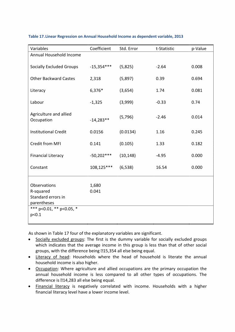
Table 17. Linear Regression on Annual Household Income as dependent variable, 2013


Annual Household Income


Other Backward Castes 2,318 (5,897) 0.39 0.694

Literacy 6,376* (3,654) 1.74 0.081

Labour -1,325 (3,999) -0.33 0.74

Agriculture and allied Occupation -14,283**

(5,796) -2.46 0.014


Credit from MFI 0.141 (0.105) 1.33 0.182

Financial Literacy -50,202*** (10,148) -4.95 0.000

Constant 108,125*** (6,538) 16.54 0.000

Observations 1,680

R-squared 0.041


*** p<0.01, ** p<0.05, * p<0.1

As shown in Table 17 four of the explanatory variables are significant.

Socially excluded groups: The first is the dummy variable for socially excluded groups which indicates that the average income in this group is less than that of other social groups, with the difference being ₹15,354 all else being equal.

Literacy of head: Households where the head of household is literate the annual household income is also higher.

Occupation: Where agriculture and allied occupations are the primary occupation the annual household income is less compared to all other types of occupations. The difference is ₹14,283 all else being equal.

Financial literacy is negatively correlated with income. Households with a higher financial literacy level have a lower income level.

Proportion of Income Generated by Occupation Type In addition to the regression analysis an additional indicator considered under household income is the distribution of income by the type of occupation that is earned from. This indicator can be used to assess whether the program causes any income diversification. Figure 45: Proportion of income earned from various occupations types across states, 2013

As shown in Figure 45, the contribution of “other occupations” to overall income is highest. Enterprises, particularly those in agriculture, contribute little to the income in Karnataka. In UP the proportion of income earned from enterprises is slightly higher with 28% of the income being earned from agricultural and allied enterprises and 26% from non-agricultural enterprises. Household Expenditure Another outcome indicator used in the analysis is household expenditure. The amount of expenditure and the item it is spent on can indicate changes in economic well-being of the household. For example, increased spending on education and other productive purposes can be considered as a sign of positive impact if attributable to the program. Additionally household expenditure is also a proxy for income. Results from a linear regression analysis using Annual Household expenditure as the dependent variable are presented in Table 18.

28%

16%

26%

20%

82%

47%

69%

0% 20% 40% 60% 80% 100%

Karnataka

UP and Uttarakhand

Overall

Proportion of Income by Occupation Types

Income from Agricultural and Allied Enterprises


Other Occupations N: Karnataka= 840, UP and Uttarakahnd = 840

Table 18. Linear Regression on Annual Household Income as dependent variable, 2013


Annual Expenditure


Other Backward Castes -9,081*** (2,853) -3.18 0.001

Literacy 4,274** (1,768) 2.42 0.016

Labour -2,139 (1,935) -1.11 0.269

Agriculture and allied Occupation -10,780***

(2,804) -3.84 0.000

Institutional Credit 0.0180*** (0.00646) 2.78 0.005

Credit from MFI 0.174*** (0.0510) 3.41 0.001

Financial Literacy -19,561*** (4,910) -3.98 0.000

Constant 89,984*** (3,163) 28.45 0.000

Observations 1,680

R-squared 0.060


*** p<0.01, ** p<0.05, * p<0.1

The explanatory power of this model is low however, statistically significant variables include:

Caste: Households from socially excluded groups and OBC households have a lower annual expenditure level compared to other groups, with the difference being ₹ 15,476 and ₹ 9,081 respectively all else being equal.

Primary occupation: Those working in agriculture and allied areas as a primary occupation also have less expenditure compared to other occupations with the difference being ₹10,780 all else being equal.

Institutional credit: The institutional credit variable is positive and statistically significant. For each additional rupee of credit, expenditure increases by 1 paisa. Thus the coefficient is small but the result is significant at 99% confidence level.

Credit from MFI is also positively correlated but has a larger coefficient. The result means that for each additional rupee of MFI credit the household gets, expenditure goes up by 17 paise.

Financial literacy is significant and negatively correlated. It shows that households with higher level of financial literacy have a lower level of expenditure.

Annual household Expenditure Pattern The distribution of household expenditure across various heads can demonstrate whether certain productive areas, such as health and education, are being prioritized in spending or not. Figure 46 depicts the average proportion of annual household expenditure that is being spent under each of these heads.

Figure 46: Annual Household Expenditure in INR disaggregated by expenditure head, 2013

The expenditure levels in Karnataka on average are much higher than UP and Uttarakhand. The former has an average annual expenditure of INR ₹1,20,000 whereas the latter has an average annual expenditure of ₹80,000. The distribution across the heads of expenditure is similar. The most significant heads of expenditure are food and provisions along with “other”. Following this the next most significant area of expense is loan repayments. The rest of heads have a roughly similar amount of annual expense.

5.3.2 Enterprises

Income accruing from enterprises is another significant outcome indicator for this Project since the scaling up of responsible microfinance is being done with the goal of enhancing livelihood opportunities in this sector through the availability of finance. The analysis presented here includes regressions and descriptive analysis. Linear Regression on Income from Enterprises Table 19 depicts the result of the linear regression analysis where income from non-agricultural enterprises was the dependent variable.

30,944 25,666 28,305

8,115

3,009

5,562

8,741

11,575

10,158

33,875

22,182

27,811

0

20,000

40,000

60,000

80,000

1,00,000

1,20,000

1,40,000

Karnataka UP and Uttarakhand Overall

An

nu

al E

xpe

nd

itu

re in

INR

Food and Provisions House Rent Utilities Communications

Travel Expenses Liquor/Smoking/Entertainment Clothes, Footwear, Haircut Festivals/Functions

Education Related Insurance Premiums Loan Repayments Health Related

Home Related Other N: Karnataka= 840, UP and Uttarakahnd = 840

Table 19. Linear Regression results for Income from Non-Agricultural Enterprises as Dependent

Variable, 2013



Socially Excluded Groups -2,119 (2,356) -0.9 0.369

Other Backward Castes 3,017 (2,385) 1.26 0.206

Literacy 897.9 (1,478) 0.61 0.544

Labour -36,058*** (1,618) -22.2 9 0.000

Agriculture and allied Occupation -36,895***

(2,344) -15.74 0.000

Institutional Credit -0.00636 (0.00540) -1.18 0.239

Credit from MFI 0.148*** (0.0426) 3.48 0.001

Financial Literacy 10,260** (4,105) 2.5 0.013

Constant 35,244*** (2,644) 13.33 0.000

Observations 1,680

R-squared 0.286


*** p<0.01, ** p<0.05, * p<0.1

There are four statistically significant dependent variables.

Primary occupation: Households with labour as primary occupation have a negative coefficient indicating that for such households, income from non-agricultural enterprises will be less. Similarly for where agriculture and allied occupations are primary the income from non-agricultural enterprises will be less.

Credit from MFI is positively correlated with income from non-agricultural enterprises. For each additional rupee of credit, income increases by 14 paise.

Financial literacy is also significant and positively correlated with income from non-agricultural enterprises indicating that greater knowledge of financial services and products can translate into better outcomes in terms of income.

Enterprise Ownership In addition to the regression analysis another indicator of change would be the proportion of the sample that owns an enterprise. Figure 47 depicts the enterprise ownership levels in the sample by state.

Figure 47: Enterprise ownership

A majority of the households in UP and Uttarakhand own some form of enterprise (agricultural and non-agricultural included). This is much higher than in Karnataka where only about 22.3% of the households in the survey sample owned an enterprise.

5.4 Financial Indicators

The main aim of the Project is to deliver microfinance products to underserved areas and to also address the gaps in the quality of microfinance service by focusing on responsible microfinance. Thus, as a part of the evaluation another set of outcome indicators that need to be included in the analysis are indicators on the status of financial literacy, access and utilization of credit (and its purposes), as well as access and utilization of other financial products such as savings and insurance. In this section the baseline status of the above listed indicators is presented.

5.4.1 Financial Literacy Financial literacy refers to knowledge of financial products and practice and here it is measured by using a financial literacy score. The financial literacy score is calculated by taking the average of responses on various questions on awareness about interest rates, credit, savings and insurance sources, and knowledge and practice related to budgeting and savings. The responses are coded as 0 for unplanned and irregular behaviour and as 1 for planned and regular behaviour. Some of the responses on awareness are coded as

22.3%

54.3%

0%

10%

20%

30%

40%

50%

60%

Karnataka UP and Uttarakhand

Pe

rce

nt

of

Ho

use

ho

lds


proportion of total possible sources of which the respondent has knowledge. Based on this a final financial literacy score is calculated on a scale of 0 to 1, with 1 being highest possible level of financial literacy and 0 being the least. Table 16 depicts the average financial literacy score of the sample in the two geographical locations being covered by Sonata – Karnataka and UP & Uttarakhand. The sample from Karnataka is 840 households and then there are 840 households from UP and Uttarakhand together. Table 20. Average financial literacy score


Average Financial Literacy Score 0.64 0.64 0.64

Standard Deviation 0.19 0.15 0.17 Maximum 0.94 0.95 0.95

Minimum 0.17 0.14 0.14

N 840 840 840

The average financial literacy score for the states, as shown in Table 20, is identical, as is the maximum and minimum. The respondents are aware of about 64% of the codified practices and products across the two locations. The standard deviation is also similar for both groups.

5.4.2 Savings In addition to credit another product that MFI clients can avail is savings. Access to formal institutions of saving can provide the household additional income (in the form of interest). This section discusses some key indicators related to savings practices. Households availing savings The first indicator is the proportion of sample households that have opted to save (either in formal or informal sources).

Figure 48: Percentage of households saving money, 2013

The proportion of households saving money is slightly higher in UP and Uttarakhand (80%), relative to Karnataka (69%). Overall about 74% o the households save which is similar to the numbers in the RCT sample. Source of Savings The second indicator is associated with the source where the savings are made. This could be a formal source like the bank or post office or informal sources such as friends and relatives. Formal sources are considered more reliable. Figure 49 shows the findings from baseline. Figure 49: Proportion of Households having savings disaggregated by Source, 2013

69%

80% 75%

0%

10%

20%

30%

40%

50%

60%

70%

80%

90%


Pe

rce

nt

of

Sam

ple

Ho

use

ho

lds

32%

17% 24%

87%

48%

66%

15%

67%

43%

0%

10%

20%

30%

40%

50%

60%

70%

80%

90%

100%


Pe

rce

nt

of

Ho

use

ho

lds

wit

h S

avin

gs

MFI Formal Sources Informal Sources

N: Karnataka=840, UP and Uttarakhand = 840

N: Karnataka=580, UP & Uttarakhand = 673, Overall = 1253

There are significant differences in the patterns across the states. In UP a larger proportion of the households save in informal sources whereas in Karnataka most of the households saved in formal sources (875). Overall the proportion of households making their savings with MFIs is the least.

5.4.3 Credit Access to Credit Access to credit refers to the households accessing loans through either formal or informal sources. The first indicator listed here is the number of outstanding loans accessed by the households in the sample. Figure 50: Percent of Sample Households having Outstanding Loans, 2013

As shown in Figure 50 across the states a majority of the households have at least 1 loan. In Karnataka a substantial proportion (22.3%) has two outstanding loans as well. Compared to the RCT sample more households have already taken out loans in this sample. Figure 51 depicts the sources from which these outstanding loans have been availed. The sources have been categorized as MFI, Formal and informal sources.

21.9% 31.8% 26.8%

54.3%

65.0% 59.6%

22.3%

3.0% 12.6%

0.2% 0.0% 0.1%

0%

10%

20%

30%

40%

50%

60%

70%

80%

90%

100%


Pe

rce

nt

of

Ho

use

ho

lds

None One Two Three Four

N: Karnataka=840, UP & Uttarakhand = 840

Figure 51: Sources from which loans are availed as a percent of loans availed. 2013.

There is large variation in the data between the states. While in Karnataka there is substantial access to all three types of sources in UP and Uttarakhand a majority of the outstanding credit (78% of loans) have been availed from MFIs. A small percentage – 2% and 6% respectively – is availed from formal and informal sources. In Karnataka the highest percentage is also availed from MFIs at 37%, however, formal sources have nearly equal amount of penetration at 36% of all loans. Figure 52 depicts the number of sources from which loans have been accessed across the two geographic locations.

37%

78%

57%

36%

2%

19%

12% 6%

9%

0%

10%

20%

30%

40%

50%

60%

70%

80%

90%


Pe

rce

nt

of

Loan

s av

aile

d

MFI Formal Informal


Figure 52: Number of sources of loans from which loans have been accessed by sample

households. 2013.

In UP and Uttarkhand the proportion of households with no access to credit is 15.48%, which this percentage is slightly higher in Karnataka at 25.83%. A large proportion of the sample households in both states have availed loans from only one source – 80% in UP and Uttarakhand and 52% from Karnataka. Types of sources for availed loans by Social Status, Religion and PPI The type of sources of credit one has access to can be affected by the social or economic profile of the household. To test this in this section results are also presented on the distribution of the various types of sources across the sample households by social status, religion and Progress out of Poverty Index of the household. Figures 53 and 54 and Table 21 depict the results by social status, religion and table by PPI respectively.

25.83% 15.48% 20.65%

52.02% 80.24% 66.13%

20.83%

4.05% 12.44%

0%

10%

20%

30%

40%

50%

60%

70%

80%

90%

100%


Pe

rce

nt

of

ho

use

ho

lds

0 Sources 1 Source 2 Sources 3 Sources 4 Sources


Figure 53: Percent of households availing credit from various sources, by social status. 2013.

The above figure depicts the distribution of access to loans from various sources within different social groups. The access to loans from formal sources is highest in the other group at 40%. Relatively in all the other social groups (SC, ST and OBC) the percentage of households availing formal credit is much less at 13% to 19%. A much higher percentage of households in these groups have availed credit from MFIs at 50% to 60% of all households. This shows a clear difference in the credit availed by households belonging to these three groups as opposed to the other group (which includes general households). Figure 54: Percent of households availing credit from various sources, by Religion. 2013.

Figure 54 shows that Muslim households are more dependent on credit from MFIs compared to all other demographics in the sample. The sample size for Sikh households is

60%

50%

61%

38%

13% 16%

19%

40%

10% 9% 6%

14%

0%

10%

20%

30%

40%

50%

60%

70%


Pe

rce

nt

of

Ho

use

ho

lds

MFI Formal Informal

55%

64%

37%

25% 21%

14%

32%

25%

10% 7%

11%

0% 0%

10%

20%

30%

40%

50%

60%

70%

Hindu Muslim Christian Sikh

Pe

rce

nt

of

Ho

use

ho

lds

MFI Formal Informal

N: SC= 741, ST = 44, OBC = 689, Other = 3

N: Hindu= 1201, Muslim = 449, Christian = 19, Sikh = 8

very small and therefore cannot be extrapolated to the general public. For Hindu households too MFIs are the most common source for access to credit at 55% of all households availing credit from MFIs. Table 21 depicts the average PPI score for households availing credit from each of these sources. Table 21. Average PPI Score

Average PPI of those availing loans

Average PPI for those not availing loans

N

Availing Not-availing

MFI 44.42 47.29 965 715

Formal 52.02 44.14 320 1360

Informal 44.03 45.80 149 1531

The average PPI size is highest for those households which have atleast one outstanding loan from a formal institution. This indicates that a higher economic status is generally associated with those who are able to access loans from formal sources. On the other hand the PPI score for those accessing MFI and informal sources is much lower at 44 points indicating a lower economic status. Average size of Outstanding and Repaid Loans by source Apart from the proportion of households that have availed loans, the size of the loan and the contribution of the different type of sources to it is also an important outcome indicators. It is expected that by going to underserved areas MFIs will reduce dependence on informal sources and encouraging borrowing from MFIs and other formal sources.

Figure 55: Average Size for Outstanding loans in Sample Households, 2013

13,504 13,504

57,515 32,071 56,486

59,660

14,597

48,561

25,965

14,236

18,473

0

20,000

40,000

60,000

80,000

1,00,000

1,20,000

1,40,000

1,60,000


Overall

Ave

rage

Lo

an S

ize

in IN

R

Unspecified Formal Sources Informal Sources MFI

N: Unspecified= 27, Formal = 346, Informal = 203, MFI = 1063

The average loan size, for all sources, is much smaller in UP and Uttarakhand compared to Karnataka. Loans from formal sources tend to be the largest on average, while loans from MFIs are the smallest on average. Figure 56 depicts the average size of repaid loans. Figure 56: Average Loan size for repaid loans, 2013

In terms of repaid loans the size of formal loans in UP and Uttarakhand is higher than that in Karnataka. Overall, MFI loans tend to be the smallest followed by formal sources for repaid loans. The average size of the MFI repaid loans is similar across the states. Table 22. Weighted average cost of credit

Weighted Annual Cost of Credit

N

Karnataka 14% 655

UP and Uttarakhand 26% 732

Overall 20% 1387

The weighted average cost of credit, as shown in Table 22, is 14% in Karnataka, and 26% in UP and Uttrakhand In Table 23 the weighted average cost of credit is further analyzed by the type of source credit has been availed from. The averages are in % per annum.

18,243

28,333 18,320

38,710

16,881 35,210

16,321 12,673 15,778

0 10,000 20,000 30,000 40,000 50,000 60,000 70,000 80,000 90,000

1,00,000


Overall Ave

rage

re

pai

d lo

an s

ize

in IN

R

Unspecified Formal Sources Informal Sources MFI

N: Unspecified= 6, Formal = 393, Informal = 131, MFI = 625

Table 23. Weighted Average Cost of Credit in percent per annum by Source of Credit, 2013


MFI 11.02 31.11 24.60

Formal 13.05 21.64 13.43

Informal 25.51 10.82 22.82

Friends/Relatives and Neighbours 19.95 3.78 13.66

N 655 732 1387

There is a significant difference in the cost of credit in the two geographic locations. In UP credit accessed from MFIs and formal sources is generally higher at 31.11% per annum and 21.64% per annum respectively. On the other hand in Karnataka credit from informal sources is much higher at 25% per annum as well as from friends and relatives at 19.95% per annum. Some of the outliers were taken out of this calculation as they were skewing the results heavily. The Figure 57 depicts the ranges of interest within which loans from the above mentioned sources (MFI, formal, informal, and friends and relatives) fall. The figure indicates how frequently loans acquired from a particular source have a high or low cost. Figure 57: Percent of loans availed falling into various cost of credit categories, 2013

The cost of credit used in the Figure 57 is the weighted average cost of credit, where the interest rate is weighed by the size of the loans. The results show that for a majority of the loans from friends, relatives and neighbours the interest rate is the least falling into the less than 10% range. This is followed by the formal loan source where 35% of all availed loans are for less than 10% per annum weighted average cost of credit. Loans from MFIs and from

16%

35% 25%

51% 7%

23%

3%

5% 74%

40%

44%

34%

0% 0%

13%

4% 2% 2%

14% 5%

0%

10%

20%

30%

40%

50%

60%

70%

80%

90%

100%

MFI Formal Informal Friends/Relatives / Neighbours

Pe

rce

nt

of

Loan

s A

vaile

d

Less than 10% 10% to 20% 20% to 30% 30% to 40% More than 40%

N: MFI= 965, Formal = 320, Informal = 63, Friends/Relatives/ Neighbours = 91

informal sources tend to be more “expensive” with 74% of the MFI loans falling into the 20% to 30% interest rate range. For informal sources 44% of all availed loans are in the 20% to 30% range, and a substantial proportion (13% and 14% respectively) also fall into the 30% to 40% and more than 40% range.

Purpose of Loan The purpose for which credit is used is a significant part of the analysis as it indicates whether the credit acquired is being used for productive purposes. Figure 58 depicts the results for the two states.

Figure 58: Purpose of loan

In this sample there is significant variation by the state. In Karnataka household cashflow, others and children’s education were mentioned as the most common purposes for which loans are taken. On the other hand in UP and Uttarakhand starting a new business, purchase of household assets and resolving cashflow problems in business are the most commonly mentioned responses. In Karnataka there is little investment in businesses with the credit acquired. Terms and Conditions To further analyze the types and forms in which credit is being availed in the study area the terms and conditions associated with these loans are also analyzed. For example this section

8% 7% 5%

4%

16%

6%

9%

6%

2%

23% 24%

1%

17% 14%

5%

0% 0% 2%

0% 0% 0%

5%

10%

15%

20%

25%

30%

Star

t a

Bu

sin

ess

New

ass

ets

for

bu

sin

ess

Ho

use

ho

ld a

sset

s

Cas

hfl

ow

in b

usi

nes

s

Ho

use

ho

ld c

ash

flo

w

Rep

ay O

ld L

oan

s/In

tere

sts

Ch

ildre

n's

Ed

uca

tio

n

Hea

lth

Exp

ense

s

To lo

an t

o s

om

eon

e el

se

Oth

er

Pe

rce

nt

of

Ho

use

ho

lds

wit

h L

oan

s av

aile

d


N: Karnataka = 636, UP and Uttarakhand = 686

includes an analysis of the additional charges and the repayment schedules. The following table depicts the average additional charges per loan by the type of source accessed. Table 24. Average additional charges per loan by source of the loan. 2013


Formal 110.20 580.81 147.16

Friends/Relatives/Neighbours 45.85 26.63 39.21

Informal 138.59 56.75 130.20

MFI 116.73 59.54 77.95

N 864 763 1627

Additional charges on average are least for loans acquired from friends and neighbours while they are highest for loans from informal sources in Karnataka (₹110) and from formal sources in UP and Uttarakhand (₹580). Figure 59 depicts the loan duration as a percentage of all availed loans. Figure 59: Loan duration for availed loans as a percentage of total number of loans availed. 2013

Almost a majority of the loans (47% to 49%) are for a 6 to 12 months duration. In UP and Uttarakhand an almost similar proportion (45%) have a duration of 1 to 2 years. On the other hand in Karnataka 25% of the loans are for a duration of more than 2 years. This is possibly due to the higher proportion of loans from MFIs availed in UP and Uttarakhand at baseline.

47% 49% 48%

22%

45% 33%

25%

1% 14%

0%

10%

20%

30%

40%

50%

60%

70%

80%

90%

100%

Karnataka UP and Uttarakhand Grand Total

Pe

rce

nt

of

avai

led

loan

s

Less than 3 Months 3 to 6 Months 6 to 12 Months

1 to 2 years More than 2 Years Don't Know

N: Karnataka = 864, UP & Uttarakhand = 763

Figure 60: Repayment schedule of loans as a percentage of total availed loans. 2013.

Of all the loans currently availed by the sample households in this study a majority of them are paid back weekly – particularly in UP and Uttarakhand where this proportion is 82%. This matches the proportion of households in UP dependent on MFIs (which is discussed in the access to credit section). On the other hand in Karnataka almost equal proportions of loans are paid back weekly or monthly. This is reflective of the higher presence of formal credit in Karnataka. Repayment Status An additional indicator under credit related practices is current repayment status on loans. The following figure depicts the results from this sample.

47.3%

82.8% 64.0%

40.7%

5.1% 24.0%

0% 10% 20% 30% 40% 50% 60% 70% 80% 90%

100%


Pe

rce

nt

of

avai

led

loan

s

Daily Weekly Fortnightly

Monthly Quarterly Half-Yearly

Annually No Specific Schedule Don't Know


Figure 61: Repayment status of loans as a percentage of total loans availed. 2013

In the patterns of repayment status as well there are significant differences between Karnataka and UP and Uttarkhand. While in Karnataka a majority of the loans are regularly paid without dues, in UP and Uttarakhand a majority (63.8%) are paying their loans with more than 1-2 pending dues. In Karnataka there are 14% of loans which are being regularly paid back with 1-2 dues pending. Satisfaction with Credit To assess the effectiveness of the delivery of “responsible” microfinance the households were asked certain questions regarding their experience and satisfaction with financial services and products available. A Satisfaction score was generated through a set of questions ranging from flexibility, understanding of terms to interest rates. Figure 62 depicts the results for satisfaction score across the three types of sources available.

82.4%

26.6%

56.4%

14.3%

5.7%

10.3%

0.5%

63.8%

30.0%

0% 10% 20% 30% 40% 50% 60% 70% 80% 90%

100%


Pe

rce

nt

of

Loan

s A

vaile

d

Regularly Paid and no Dues Regularly paid and one or two dues pending

Paying, more than one or two dues Irregular and occasional payment

Stopped Repaying Don't Know


Figure 62: Average Satisfaction score for credit services and products offered across various

sources, (Sonata 2013)

Figure 62 shows that the satisfaction levels with the various types of sources are largely similar across all the parameters except for processing and add on services. Respondents reported a lower level of satisfaction with processing in informal sources compared to MFIs and formal sources. On the other hand formal sources did not rank as high as the other two in the area of add-on services. The FGD discussion from this study on credit needs and availability are similar to those from the groups of the RCT study. In the study area there are a number of MFIs that operate. The participants are able to name the MFIs. Due to the large numbers, most groups say that they take loans from MFIs for small business. One group said that they get loans from MFIs for house reconstruction and weddings also. For emergency needs they go to money lenders. Most participants understand the processes of MFIs, however, they know the repayment schedule but not necessarily the interest rate. People who do not take loans from MFIs usually do so because of the procedure and rules. By and large the satisfaction with MFIs was high, with participants saying that before MFIs and SHGs they had few options for affordable loans. Most of the participants say that they have phone number of offices, but incidents of grievance have not occurred till now. One group said that even if they have problems they don’t complain.

5.4.4 Investment in Enterprise An additional level of outcome indicators that have to be considered in this study is the use of credit for productive purposes. As per the theory of change the use of the products and services offered by the Project should lead to an increased investment in enterprise from the households leading to better well-being. Thus one of the outcome indicators included in the analysis will be quantum of investment being made into enterprises and the sources it is accessed from.

0

0.2

0.4

0.6

0.8

1

Access to Credit Services

Processing

Collateral

Interest Rate

Flexibility of Repayment Options

Credit Limit

Terms and Conditions

Add On Services

Formal

Informal

MFI

N: Formal=549, Informal =827, MFI = 1114

Investment per Enterprise The first indicator is the average investment made into an enterprise (in Rupee value). Figure 63 depicts the average size of investment into enterprises for each household (regardless of the number of enterprises). Figure 63: Average investment in Enterprises per household, 2013

The average amounts invested in enterprise across the states are similar. Overall the average is slightly higher in Karnataka compared to UP and Uttarakhand. Source of Investment Apart from encouraging investment in enterprise, a goal of the project is also to reduce dependence on informal sources for enterprise investment. In this section this is measured in two ways. The first is to look at the proportion of enterprises that have been set-up using loans from various types of sources and is depicted in figure 64. The second indicator is the distribution of the value of investment by source of credit. In these graphs only those households are considered who have a business and who have opted for credit to finance them.

29452

24370 25801

0

5000

10000

15000

20000

25000

30000

35000


Ave

rage

inve

stm

en

t in

En

terp

rise

pe

r h

ou

seh

old

(in

INR

)

Average Investment per Household in Enterprise

N: Karnataka=178, UP & Uttarakhand= 454, Overall = 632

Figure 64: Proportion of Enterprises funded by each type of source, 2013

A majority of the enterprises across states are funded by loans acquired through formal sources. This is followed by a much smaller proportion (14.3 % in Karnataka and 0% in UP and Uttarakhand) having formal and informal sources both being used to fund the enterprise. None of the enterprises have investments acquired through MFIs in the sample. Figure 65: Value invested in enterprise from each source as a percent of total investment, 2013

Though the number of formal loans being used to finance enterprises is higher than all others the amount being sourced from them isn’t. Here investment that combines informal and formal loans together is of a larger size. The smallest is MFI and Formal both.

78.6%

100.0%

82.4%

14.3%

0.0%

11.8% 7.1%

0.0% 5.9%

0%

10%

20%

30%

40%

50%

60%

70%

80%

90%

100%

Karnataka Uttar Pradesh Overall

Pe

rce

nt

of

tota

l en

terp

rise

s

Formal Informal and Formal Both MFI and Formal Both

31.6%

100.0%

28.6%

51.3%

0.0%

53.5%

17.1% 0.0%

17.8%

0%

10%

20%

30%

40%

50%

60%

70%

80%

90%

100%

Karnataka Uttar Pradesh Total

Inve

stm

en

t A

mo

un

t fr

om

eac

h s

ou

rce

as

a p

erc

en

tage

of

the

to

tal i

nve

stm

en

t

Formal Informal and Formal Both MFI and Formal Both

N: Karnataka=65, UP & Uttarakhand= 149, Overall = 214

N: Karnataka=65, UP & Uttarakhand= 149, Total = 214

6 KEY MESSAGES FROM THE BASELINE STUDY (RCT AND NON-RCT) The baseline study has established the status of the impact, outcome and program indicators for different samples The baseline indicates that:

The project is target profiles that are deserving, given the status of impact indicators

Level of financial literacy low

Current level of access to credit seems limited; also the institutional credit

Cost of credit ranges widely; goes up to 10% p.m.

Level of access to insurance also low MFI is the preferred source for credit for enterprise but quantum of loans available from MFI is small, and loans are not necessarily structured to meet the credit needs of the poor. They are still compelled to depend on informal sources for their needs. Grievance mechanisms not completely developed. This results in some suspicion, especially if there is a feeling of being cheated. Towards this greater communication and frequent financial literacy related activities are required. Satisfaction with MFI is moderate, particularly on flexibility of repayment and credit limit. This also prevents people from using MFI for enterprises that do not have regular and periodic returns from enterprise.

ANNEXURE A: TIMELINES AND DISCUSSIONS ON MFI SELECTION

No

Date Details

1 04-Nov-11 First formal interaction between SIDBI and CMS 2 16-17 Nov-11 For SIDBI: Engaging with CMS team; learning about study design

and methodology For CMS: Engaging with SIDBI team; obtaining details about programme relevant to the study

3 18-Nov-11 For World Bank: Engaging with CMS; learning about study design and methodology For CMS: Engaging with SIDBI team; obtaining details about programme relevant to the study; clarifying points related to programme and study; defining study purpose

4 07-Dec-11 CMS submitted a note documenting processes till data and a proposed methodology (attached in Annex A)

5 22-Dec-11 Clarify methodology(proposed by CMS in note submitted on 07 Dec), Implications of the design for programme side

6 29-Dec-11 CMS submitted a new methodology note with two design options – one being the same as previously proposed and another being an experimental design (attached in Annex B)

7 8 9 10 11 12 13 14

20-Jan-12 21-Mar-12 31-Mar-12 15-Jun-12 31-Dec-12 5-Jan-13 10-Mar-13 9-Apr-13

SIDBI indicates the experimental design is preferable to understand the impact World Bank provides go ahead and inception report is submitted by CMS Secondary data analysis completed Discussions with 2 MFI on the design and pilot completed. 5 MFIs finalised for the study by SIDBI Discussions with 5 MFI on the design, convincing on the merits of RCT, encouraging MFIs to participate in the study. The 3 MFI which agreed to be part of the study took considerable time to provide the list of samples as MFIs’ board approval was required. Update on the status of the assignment and progress sent to SIDBI by CMS Data collection for 3 MFI completed Presentation to World Team in Bangalore on initial baseline finding

No

Date Details

15 16 17 18 19 20 21

15-Apr-13 18-Apr-13 18-Jun-13 30-Sept-13 20-Oct-13 31-Jan-14 20-Feb-14

Agreement on change in design for the 2 MFIs with World Bank Note on change in study design sent to SIDBI by CMS Formal approval from SIDBI received on the change in the design 2 MFIs identified by SIDBI and informed to CMS Discussions with the 2 MFI on the design Data collection for the 2 MFI collected Data entry for all the records collected from MFI completed

The discussions with each of the MFIs and time which took for the MFIs to agree or disagree with the design is given below

State: Uttar Pradesh Originally selected MFI: Cashpor MFI selected now: Margadarshak Efforts from SIDBI and CMS: 1. Cashpor was provided with the design presentation Clarifications were provided for the methodology The discussions with Cashpor initiated in Feb 2012. The final decision of Cashpor for not participating in the study provided in the month of Oct 2012. In the month of Oct 2012, the MFI was changed to Margadarshak. Reasons for change: Cashpor has been consolidating its branches and has no plans for expansion in the year 2012-13. In the absence of new branches, the MFI cannot take part in the study as the study design requires new branches.

Margdarshak was selected as it is expanding in few areas in UP and was willing to participate in the study.

State: Bihar Originally selected MFI: Ujjivan MFI selected now: NA Efforts by SIDBI and CMS: Discussions started with Ujjivan in the month of April 2012 Initial acceptance by Ujjivan provided in June 2012 Follow up discussions on selection of location went till Jan 2013. The final decision by Ujjivan not agreeing to part of the study came on 28th Jan 2013. Reasons for change: Ujjivan has indicated their unwillingness to participate in the study

State: West Bengal and Orrisa MFI originally selected: Bandhan Efforts by SIDBI and CMS: Discussions started with Bandhan in the month of June 2012 Initial acceptance by Bandhan provided in June 2012 Follow up discussions on selection of location went till Sept 2012. The final decision by Bandhan not agreeing to part of the study came on October 2012. Reason for change: Bandhan has no plans of expansion in the respective states. No other MFI was selected as identification of MFI working in the states coupled with willingness to participate in the study was felt to be doubtful.

State: Madhya Pradesh MFI Originally selected: BSFL MFI selected now: Equitas and Sonata Efforts by SIDBI and CMS: Discussions started with BSFL held Reasons for change: BSFL has no plans for expansion Equitas and Sonata were willing to participate and have plans to open new branches.

State: Maharashtra MFI originally selected: Equitas MFI selected now: Sangamitra Reasons for changes: Equitas has plans of expansion in the state of MP rather than Maharashtra Sangamitra has opened new branches in Maharashtra and is willing to participate in the study.

Following this, in the month of April 2013, discussions were held with World Team in Bangalore, Karnataka on the 9th April 2013. The preliminary finding presentations were made by CMS. During the discussions and presentation the following were noted:

1. The random sampling shows similar pattern and comparable status of indicators across the spectrum of households who will receive treatment across 3 years, 2 years and one year (as per the pipeline method agreed to).

2. The evaluation framework was shared and presented 3. Theory of Change for the program and the indicators for Impact and Outcome were

agreed and the status within 2520 household was shared. 4. Difficulties in completion of the assignment were discussed in detail. 5. The efforts made by SIDBI and CMS to get the MFIs on board were shared. 6. The non agreement with some of the MFI for the use of RCT was shared and an

alternative design was suggested to cover the balance of the 2 MFIs. 7. It was agreed that the choice of the 2 MFIs shall be made by SIDBI

Documents

IMPACT ASSESSMENT STUDY OF ASSISTED MICRO FINANCE