Impact of an increased biomass use on agricultural markets, prices and food security: A longer-term perspective

Josef Schmidhuber1

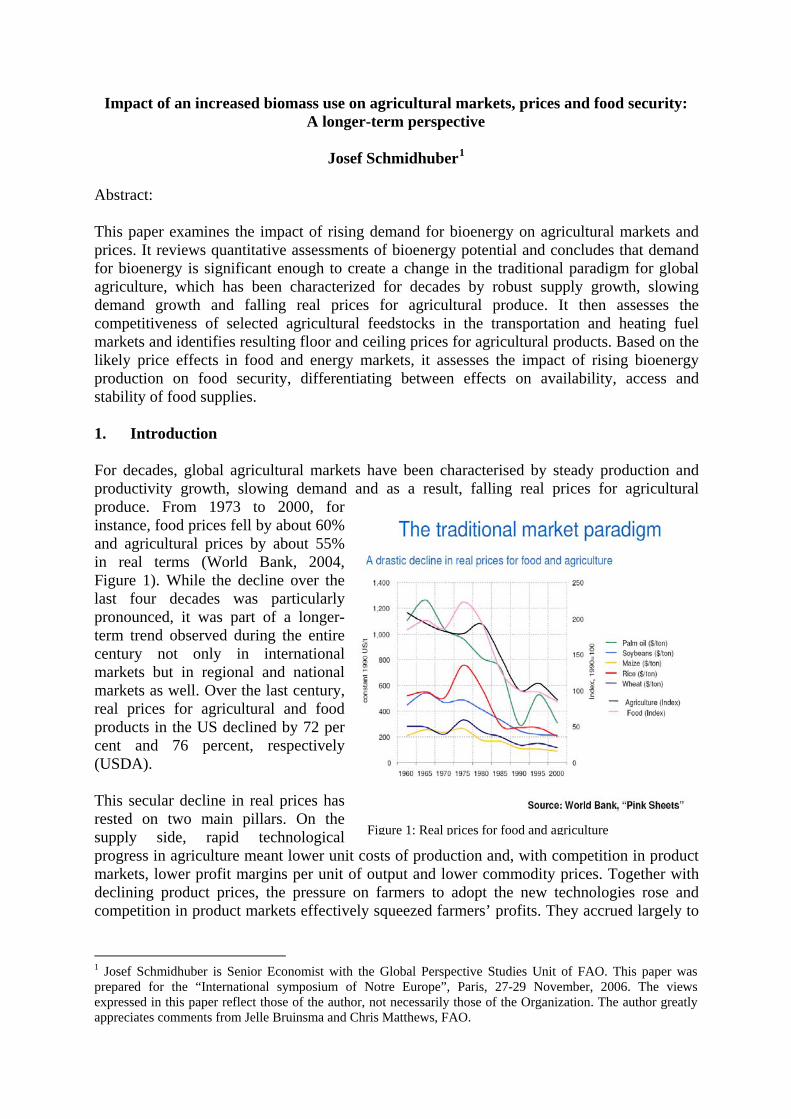
Abstract: This paper examines the impact of rising demand for bioenergy on agricultural markets and prices. It reviews quantitative assessments of bioenergy potential and concludes that demand for bioenergy is significant enough to create a change in the traditional paradigm for global agriculture, which has been characterized for decades by robust supply growth, slowing demand growth and falling real prices for agricultural produce. It then assesses the competitiveness of selected agricultural feedstocks in the transportation and heating fuel markets and identifies resulting floor and ceiling prices for agricultural products. Based on the likely price effects in food and energy markets, it assesses the impact of rising bioenergy production on food security, differentiating between effects on availability, access and stability of food supplies. 1. Introduction For decades, global agricultural markets have been characterised by steady production and productivity growth, slowing demand and as a result, falling real prices for agricultural produce. From 1973 to 2000, for instance, food prices fell by about 60% and agricultural prices by about 55% in real terms (World Bank, 2004, Figure 1). While the decline over the last four decades was particularly pronounced, it was part of a longer-term trend observed during the entire century not only in international markets but in regional and national markets as well. Over the last century, real prices for agricultural and food products in the US declined by 72 per cent and 76 percent, respectively (USDA).

Figure 1: Real prices for food and agriculture

This secular decline in real prices has rested on two main pillars. On the supply side, rapid technological progress in agriculture meant lower unit costs of production and, with competition in product markets, lower profit margins per unit of output and lower commodity prices. Together with declining product prices, the pressure on farmers to adopt the new technologies rose and competition in product markets effectively squeezed farmers’ profits. They accrued largely to

1 Josef Schmidhuber is Senior Economist with the Global Perspective Studies Unit of FAO. This paper was prepared for the “International symposium of Notre Europe”, Paris, 27-29 November, 2006. The views expressed in this paper reflect those of the author, not necessarily those of the Organization. The author greatly appreciates comments from Jelle Bruinsma and Chris Matthews, FAO.

buyers of food and agricultural products, with a consequent decrease in real costs of food and fibre products to consumers (Gardner 2002). In many countries, higher productivity in agriculture was accompanied by an intensification of production methods, i.e. higher applications of fertilizer, pesticides, and an expansion of irrigation. For most new high-productivity technologies only produced higher output if combined with higher levels of inputs. And finally, farmers tried to expand the production base. Lower profits margins per unit of output required increased volumes, more cropland and higher cropping intensities. The result was a massive increase not only in productivity but also in total output.

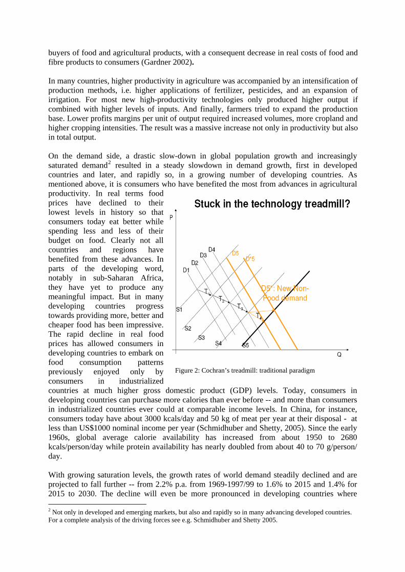
Figure 2: Cochran’s treadmill: traditional paradigm

On the demand side, a drastic slow-down in global population growth and increasingly saturated demand2 resulted in a steady slowdown in demand growth, first in developed countries and later, and rapidly so, in a growing number of developing countries. As mentioned above, it is consumers who have benefited the most from advances in agricultural productivity. In real terms food prices have declined to their lowest levels in history so that consumers today eat better while spending less and less of their budget on food. Clearly not all countries and regions have benefited from these advances. In parts of the developing word, notably in sub-Saharan Africa, they have yet to produce any meaningful impact. But in many developing countries progress towards providing more, better and cheaper food has been impressive. The rapid decline in real food prices has allowed consumers in developing countries to embark on food consumption patterns previously enjoyed only by consumers in industrialized countries at much higher gross domestic product (GDP) levels. Today, consumers in developing countries can purchase more calories than ever before -- and more than consumers in industrialized countries ever could at comparable income levels. In China, for instance, consumers today have about 3000 kcals/day and 50 kg of meat per year at their disposal -/ at less than US$1000 nominal income per year (Schmidhuber and Shetty, 2005). Since the early 1960s, global average calorie availability has increased from about 1950 to 2680 kcals/person/day while protein availability has nearly doubled from about 40 to 70 g/person/ day. With growing saturation levels, the growth rates of world demand steadily declined and are projected to fall further -- from 2.2% p.a. from 1969-1997/99 to 1.6% to 2015 and 1.4% for 2015 to 2030. The decline will even be more pronounced in developing countries where

2 Not only in developed and emerging markets, but also and rapidly so in many advancing developed countries. For a complete analysis of the driving forces see e.g. Schmidhuber and Shetty 2005.

growth in aggregate food demand is projected to fall from 4.0% p.a. to 2.2% and to 1.7% for the same periods (Bruinsma, 2003). FAO’s long-term outlook to 2050 suggests that the decline in growth will become even more pronounced after 2030, with growth rates for aggregate food demand declining to 0.9% for the world as a whole and 1.1% p.a. for the developing world (FAO, 2006). Even a rapid decline in the number of the 850 million now undernourished would not alter this outlook substantially3 in the longer term. The world could easily produce the additional food needed to feed them well, and do so without any significant “price stress” on world commodity markets. If today’s hungry are hungry it is because they are unable to purchase enough food and not because the world cannot produce enough. The potential demand is simply too small to challenge the spare production and productivity capacity of global agricultural production. Potential demand from energy markets could, however, be large enough to challenge the spare production capacity of world agriculture. How large the potential of energy markets is, how much and what type of agricultural produce is competitive in the energy markets and how this growing competition is changing price formation in commodity markets will be illustrated in this paper. It will also examine whether the non-food demand potential is large enough to stop the slow-down in overall demand growth or even reverse it. The size of the competitive potential will crucially depend on how much agricultural produce becomes a competitive source of energy in the overall energy market. At current energy prices, some agricultural feedstocks have indeed already become competitive sources of energy, at least under certain production environments. As a consequence, demand for these feedstocks has expanded and already supports prices for these commodities. Where demand was particularly pronounced as in the case of cane-based ethanol, bioenergy demand has created a quasi intervention system and an effective floor prices for agricultural produce – sugar in this case. With higher energy prices the range of products competitive in the energy markets has increased, strengthening the floor price effect for agriculture in general (Schmidhuber, 2005). In some countries, policy incentives to use and/or produce bioenergy further added to the demand for agricultural produce and lowered the parity price equivalent to a point where many otherwise uncompetitive feedstocks became economically viable in the energy market (Schmidhuber, 2006). The growing dependence of agriculture on energy markets has also created a growing concern that high and rising energy prices will create new or augment existing food security problems as a growing number of poor consumers are priced out of the food markets by rising energy demand or are exposed to more pronounced swings in food supplies and prices. This paper will show that higher prices can indeed add to food security problems, but that price increases are not open-ended and fears of a global neo-Malthusian scenario are unwarranted. The main reason for is an endogenous ceiling price effect (Schmidhuber 2006). As feedstock costs are the most important cost element of all (large-scale) forms of bioenergy use, feedstock prices (food and agricultural prices) cannot rise faster than energy prices in order for agriculture to remain competitive in energy markets (ceiling price effect). Barring massive subsidies for bioenergy, the need to maintain competitiveness should create an endogenous brake on food prices. 3 A third factor, albeit unrelated to agriculture, added to the decline in real prices over the last decade: Driven by globalization and growing competition in global manufactures markets, nominal prices for industrial goods and thus for the numéraire used to deflate agricultural prices have declined faster than nominal prices in agriculture (IMF, 2006).

Before floor and ceiling price effects are discussed in detail, it should be useful to estimate the potential size of bioenergy production and thus how far demand for agricultural produce can expand. The next section therefore examines the various potentials of bioenergy production, juxtaposes them with the overall energy markets and provides an idea as to what the regional distribution is likely to be. 2. How big is the potential for bioenergy? A number of studies have assessed the global and regional potential of bioenergy production. Their estimates differ considerably and the interpretation of the results presented has to be vetted carefully against the basic assumptions made (see e.g. Smeets et al. 2004, Fischer and Schrattenholzer, 2000). Assessments differ due to (i) different scopes in terms of countries and feedstock coverage, (ii) different assumptions made as to “reserve” resources (land, water, etc.) required to meet the world’s need for food, forest and fibre demand, (iii) different definitions of potentials (theoretical, technical, economic) or (iv) simply because they pursued completely different methodological approaches. To discuss the differences in the various studies in greater detail would exceed the scope of this paper and distract from its main purpose. Instead, the focus will be to give an idea of the magnitude of the potential and to illuminate the discussion by identifying the various forms of potentials. The analysis by Fischer and Schrattenholzer (Fischer and Schrattenholzer, 2000) helps illustrate some of the salient points that determine the various “potentials” and provides plausible estimates for their magnitude. The study is comprehensive in terms of country coverage, provides regional details and distinguishes five major possible sources of biomass, i.e. arable land, grasslands, forests, as well as animal and municipal wastes4. The study also distinguishes technical from economic potentials and takes account of cropland needs for food, forest and fibre production based on FAO’s long-term outlook for global agriculture (Bruinsma, 2003). It is therefore compatible with many other assumptions made in this paper. 2.1 The theoretical potential At the most general level, the global bioenergy potential is defined by the total amount of energy produced by global photosynthesis. Plants collect a total energy equivalent of about 3150 Exajoule, EJ [1018J/a] (Kapur, 2004) per year or nearly seven times the global current amount of energy used [total primary energy supply in 2004 was about 460 EJ (IEA, 2004a)]. While no doubt impressive, the photosynthesis potential as such is rather irrelevant for an assessment of global bioenergy potential. For one thing, it includes vast amounts of biomass that cannot be harvested because it is too inaccessible or because the cost of harvesting would be too high. For instance, nearly one third of photosynthesis, or about 1150 EJ/a, is produced as phytoplankton and other plants in the oceans (Kapur, 2004). Maritime photosynthesis products not only form the basis of the oceans’ food chains but are also difficult if not impossible to harvest. Similarly, much of what grows on land is either not harvestable (too remote, etc) or simply not available for energy use, being required for other purposes. The theoretical potential is not only limited by the global area suitable for photosynthesis production but also, and decisively so, but the low energy efficiency of photosynthesis. Plants are hugely inefficient converters of solar energy and will therefore face growing competition from more efficient methods of collecting and converting solar radiation. At around 0.5

4 Bioenergy crops and crop residues can come from both arable land and grasslands

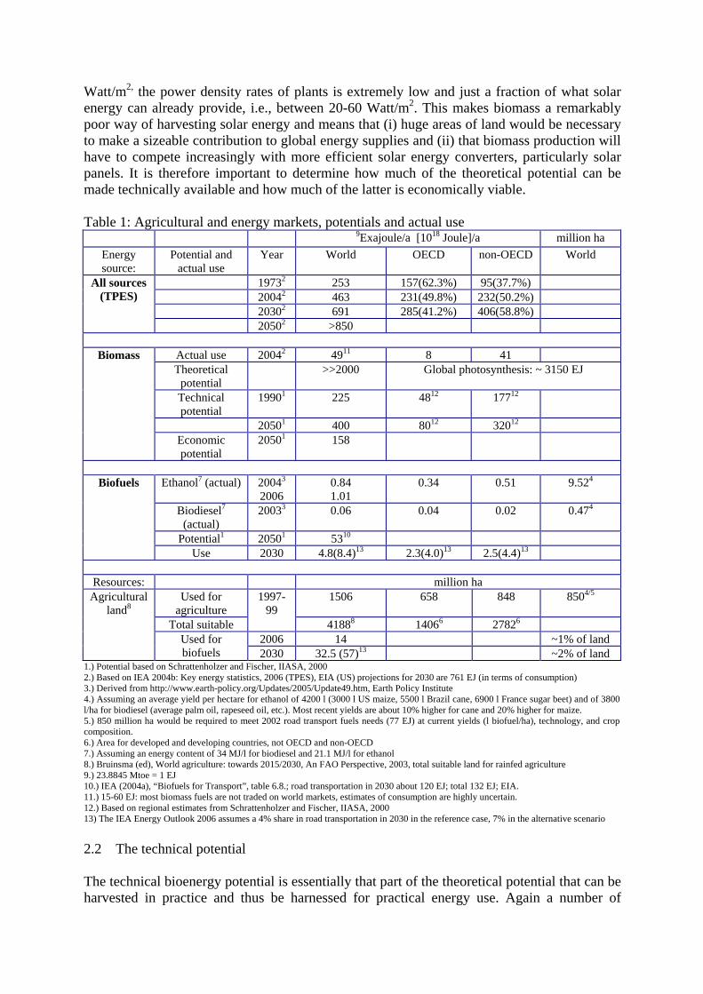
Watt/m2, the power density rates of plants is extremely low and just a fraction of what solar energy can already provide, i.e., between 20-60 Watt/m2. This makes biomass a remarkably poor way of harvesting solar energy and means that (i) huge areas of land would be necessary to make a sizeable contribution to global energy supplies and (ii) that biomass production will have to compete increasingly with more efficient solar energy converters, particularly solar panels. It is therefore important to determine how much of the theoretical potential can be made technically available and how much of the latter is economically viable. Table 1: Agricultural and energy markets, potentials and actual use

9Exajoule/a [1018 Joule]/a million ha Energy source:

Potential and actual use

Year World OECD non-OECD World

19732 253 157(62.3%) 95(37.7%) 20042 463 231(49.8%) 232(50.2%) 20302 691 285(41.2%) 406(58.8%)

All sources (TPES)

20502 >850

Actual use 20042 4911 8 41 Theoretical

potential >>2000 Global photosynthesis: ~ 3150 EJ

Technical potential

19901 225 4812 17712

20501 400 8012 32012

Biomass

Economic potential

20501 158

Ethanol7 (actual) 20043

2006 0.84 1.01

0.34 0.51 9.524

Biodiesel7

(actual) 20033 0.06 0.04 0.02 0.474

Potential1 20501 5310

Biofuels

Use 2030 4.8(8.4)13 2.3(4.0)13 2.5(4.4)13

Resources: million ha Used for

agriculture 1506 658 848 8504/5

Total suitable

1997-99

41888 14066 27826 2006 14 ~1% of land

Agricultural land8

Used for biofuels 2030 32.5 (57)13 ~2% of land

1.) Potential based on Schrattenholzer and Fischer, IIASA, 2000 2.) Based on IEA 2004b: Key energy statistics, 2006 (TPES), EIA (US) projections for 2030 are 761 EJ (in terms of consumption) 3.) Derived from http://www.earth-policy.org/Updates/2005/Update49.htm, Earth Policy Institute 4.) Assuming an average yield per hectare for ethanol of 4200 l (3000 l US maize, 5500 l Brazil cane, 6900 l France sugar beet) and of 3800 l/ha for biodiesel (average palm oil, rapeseed oil, etc.). Most recent yields are about 10% higher for cane and 20% higher for maize. 5.) 850 million ha would be required to meet 2002 road transport fuels needs (77 EJ) at current yields (l biofuel/ha), technology, and crop composition. 6.) Area for developed and developing countries, not OECD and non-OECD 7.) Assuming an energy content of 34 MJ/l for biodiesel and 21.1 MJ/l for ethanol 8.) Bruinsma (ed), World agriculture: towards 2015/2030, An FAO Perspective, 2003, total suitable land for rainfed agriculture 9.) 23.8845 Mtoe = 1 EJ 10.) IEA (2004a), “Biofuels for Transport”, table 6.8.; road transportation in 2030 about 120 EJ; total 132 EJ; EIA. 11.) 15-60 EJ: most biomass fuels are not traded on world markets, estimates of consumption are highly uncertain. 12.) Based on regional estimates from Schrattenholzer and Fischer, IIASA, 2000 13) The IEA Energy Outlook 2006 assumes a 4% share in road transportation in 2030 in the reference case, 7% in the alternative scenario 2.2 The technical potential The technical bioenergy potential is essentially that part of the theoretical potential that can be harvested in practice and thus be harnessed for practical energy use. Again a number of

studies have gauged the volume of biomass that can technically contribute to global energy supplies. Not surprisingly all estimates suggest that the technical potential is a relatively small fraction of the theoretical one. Fischer and Schrattenholzer for instance estimate that the global technical potential of bioenergy was about 225 EJ/a in 1990 and that it could increase to about 400 EJ/a by 2050. The near doubling in the potential from 1990 to 2050 largely reflects anticipated increases in crop yields and to a minor extent assumes growing amounts of municipal and agricultural wastes resulting from population growth and rapid urbanization. With about 177 EJ in 1990, non-OECD countries would account for the lion’s share of the global technical potential, Africa and Latin America together providing about 42% of that figure. In contrast, the technical potential of OECD countries, about 48 EJ, is rather limited and accounts merely for 21 percent of overall technical potential5. 2.3 The long-run economic potential More important than purely technical availability, however, is the question of how much technically-available bioenergy potential is economically viable. The two crucial parameters here are the prices of fossil energy and the costs of producing bioenergy. This means that the technical potential needs to be scaled down further to that part of the bioenergy stock that can compete with fossil energy after harvesting, transport and processing. These overheads can be substantial and accordingly reduce the amount of bioenergy that is profitable to use. Even more important is that increased use will mean that the costs of using bioenergy can and will increase rapidly at the margin of using an additional unit of biomass. How steeply long-term supply curves will increase is difficult to gauge. The increase in marginal costs of global sugar production illustrated in Figure A3 (Annex) is no doubt exaggerated by massive subsidies that keep high-costs producers in operation (right end of the curve). Though a massive increase in biomass use and thus growing competition for area should, however, also result in a rapid increase in marginal costs, once traditional production acreage is exhausted. Based on the IIASA-WEC A3 scenario, which assumes a continuation of high economic growth, rapid technological development and fossil energy prices in the middle of the existing long-term estimates, Fischer and Schrattenholzer find the economically viable potential to be in the range of 150 EJ/a globally (Fischer and Schrattenholzer, 2000). It is important to set this in the broader context of current and future energy needs. First, the 150 EJ/a should be seen in the context of future energy needs, projected at some 850 EJ/a by 2050, so that the contribution of bioenergy would “only” be around 17.5%, or only 7% above its current share of 10.6%. Second, the 150EJ/a are based on the use of biomass, not of biofuels. While second-generation biofuels should lower conversion losses and costs considerably, the 150 EJ/a would melt down to about 53 EJ/a in terms of biofuels at current conversion technologies and efficiencies (IEA, 2004a). 2.4 The current short-term economic potential The assessment of the long-term economic potential depends crucially on assumptions made about the prices of fossil energy, the development of agricultural feedstocks and future technological innovations in harvesting, converting and employing biofuels. In their current 5 It is interesting to note that the regional estimates for the potentials of bioenergy correspond almost exactly to current and actual use of biomass. This holds both for shares between OECD and non-OECD countries as well as for the distribution within OECD countries. Current use in the OECD countries for instance is about 8 EJ/a or 16% of total current biomass use. The potential is estimated to be 80 EJ/a or 20% of the total potential in 2050.

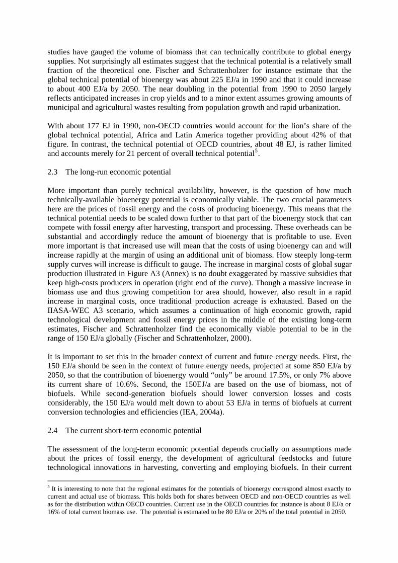
state all these factors also determine the competitiveness of the various forms of bioenergy and it should thus be useful to examine how they currently influence what feedstock is viable in what production or farming system. The key indicator in examining the question of short-term potential and economic viability is therefore the break-even point for the various forms of bioenergy and how sensitive this is with respect to fossil energy prices and most importantly agricultural feedstock prices. Break-even points are given by the so-called parity price, i.e. the price of fossil fuel per unit of energy at which the various forms of bioenergy become competitive. This indicator will be discussed in section 3 of this paper and key parity price levels will be presented. The main factor that determines the parity price of a particular form of bioenergy is the cost of the feedstock (market price adjusted for subsidies and other policy interventions that do not affect prices directly). At the industrial level of bioenergy production, feedstock costs account for the lion’s share of total costs and can exceed 80% of total production costs. As the energy market is large compared to the agricultural feedstock markets, prices of agricultural feedstocks are endogenous to changes in fossil energy prices. As also demonstrated in section 3 of this paper, large energy markets can create both a floor price for agriculture as well as ceiling price, i.e. the price for agricultural feedstocks that is still low enough to keep a given form of bioenergy in the energy market. As this price cannot be exceeded in the long-run, to keep a given feedstock viable in the energy market, the current economic potential of bioenergy is an endogenous potential that depends not only on the price changes in fossil energy markets but also, and crucially so, on the demand for and the price of the feedstocks. 2.5 Current, actual use of bioenergy The discussion of the biomass potentials suggests that the demand for biomass could create substantial demand for agricultural resources, but that the economically viable use of biomass is crucially dependent on prices for fossil energy, agricultural prices and the cost of converting biomass into marketable bioenergy. What still needs to be discussed is how much of the potential has already been reaped, what feedstocks are used and what forms of biomass are employed as the basis for bioenergy production. In 2004, global biomass6 use accounted for 49EJ or nearly 10.6% of total primary energy supply (TPES) (IEA, 2006, see also Table 1). Table 1 also shows that the importance of biomass use differs considerably across countries and groups of countries. In general, biomass is a more important contributor to energy supplies in developing countries where it accounted for nearly 19% of their TPES in 2004, equivalent to 41 EJ, while it is much less important, both in absolute terms and as a share of total energy supply, in OECD countries. In almost all developed countries it accounts for less than 5% of TPES and in 2004 represented a mere 3.4% for the OECD countries on average. While biomass accounts for small shares of TPES in almost all OECD countries, the importance varies widely across the various developing regions. Whereas biomass is entirely irrelevant for all oil and/or gas rich countries in the Near-East/North-Africa region, it is often the most important source of energy in most countries in sub-Saharan Africa. In some of these countries, bioenergy accounts for more than 90% of the TPES, examples are Tanzania (92%), Ethiopia (92.1%) and the Democratic Republic of Congo (93.5%) (for details see Figure 3).

6 Combustibles and waste

For discussion of the possible impacts of bioenergy on agricultural markets it is important to note that the major role it plays in developing countries is not a new phenomenon. The forms of bioenergy used in developing countries make that clear. They have little to do with the advanced and modern forms of bioenergy that have become en vogue in developed countries as a result of high fossil fuel prices and environmental concerns. The latter essentially reflect advanced development and demand for high-end environmental goods. In contrast, high biomass use in developing countries is often based on low-end products like charcoal, fuel wood or even cow dung and is often associated with environmental damage (deforestation) and health problems (fuel wood in India). The dominant role of these semi-marketable or non-marketable feedstocks, mostly based on forest products or by-products of agricultural production, means that the use of biomass in most developing countries has had no, or only limited, impact on international agricultural markets. The bioenergy that has most affected agricultural markets is probably biofuels, i.e. highly marketable bioenergy based on traded feedstocks such as cereals, sugar or cassava. Their use for energy production has created considerable public interest but their contribution to the energy markets is almost negligible. In 2006 they provided only about 1.1EJ or 1.3% of road transportation needs and thus less than 0.3% of total energy supplies (Table 1). As these feedstocks will play a dominant role in the supply of first-generation biofuels, the obvious question is how much land is necessary to make a sizeable contribution to current energy needs. Meeting global road transportation needs, which are about 77EJ/a or about 18% of global energy use, for instance. A mechanistic way to address this question is to assume current conversion efficiency, current yields, current feedstock composition (sugar cane, maize, rapeseed, etc.) and the proportions of bioethanol to biodiesel production and calculate the land area needed to produce 77 EJ in terms of biofuels. The resulting answer is around 850 million ha, equivalent to the total cropland currently used for food and fibre production in developing countries (Table 1). But this is unrealistic answer as it ignores the endogenous limits stemming from the fact that the demand for these feedstocks would drive up their prices and limit their use. Encroachment on existing land and expansion of overall crop land would consequently also be curtailed. The exercise is nonetheless useful as it shows that the energy market is “big” relative to the agricultural market and that energy prices will determine agricultural prices where agriculture is a competitive feedstock. When competitive, the energy market affects the agricultural markets and creates a floor price for agricultural produce but the contribution of agriculture would be too small to affect the energy market. How these floor price effects work in practice and how rising feedstock prices create a ceiling price effect for agricultural produce will be discussed in the next sections.

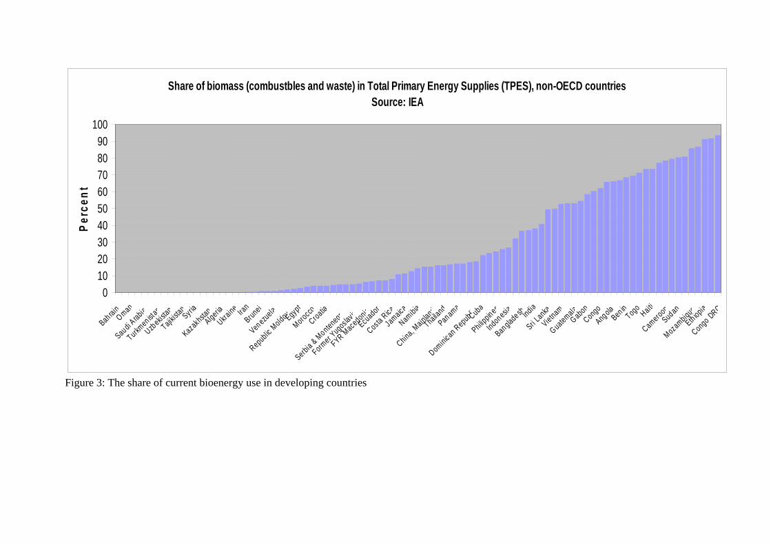
Share of biomass (combustbles and waste) in Total Primary Energy Supplies (TPES), non-OECD countriesSource: IEA

0102030405060708090

100

Bah rainOman

Saudi Arabia

Turkmen ist a

nUzbekis

tanTajiki

stan

SyriaKazakhsta

nAlgeriaUkra

ine Iran

BruneiVen ezuela

Republic MoldovaEgyptMorocco

Croatia

Serbia & Montenegro

Former Y

ugos lav ia

FYR MacedoniaEcuador

Costa RicaJamaicaNamibia

China, MainlandThailandPanama

Dominican Repub liCubaPhilip

pin esIndonesia

Banglade sh IndiaSri L

ankaVietnam

GuatemalaGabonCongoAngola

Ben inTogo

HaitiCameroon

SudanMozambique

Eth iopiaCongo DRC

Perc

ent

Figure 3: The share of current bioenergy use in developing countries

3 Price effects

3.1 Higher fossil fuel prices create a floor price for agricultural products

Agricultural prices have always been affected by energy prices. Hitherto, this price link was largely limited to the impacts of higher energy prices on the prices of agricultural inputs, i.e. the prices for fertilizer, pesticides, or diesel. Higher input prices often resulted in a rationalisation of production and thus lower output. This has changed. With rapidly rising energy prices and improved bioenergy conversion technologies, higher energy prices are also affecting agricultural output prices. As prices for fossil energy reach or exceed the energy equivalent of agricultural products, the energy market creates demand for agricultural products. Where demand from the energy sector is large/elastic and agricultural feedstocks are competitive in the energy market, a floor price effect for agricultural products results. The output price effect creates incentives to produce more rather than less.

How big is demand from the energy sector?

The effectiveness of this floor price mechanism strongly depends on the volumes of agricultural output/feedstocks that can be absorbed by the fuel market, i.e. on demand from the energy sector being sufficiently large. As illustrated in section 2, the volume of global demand for energy is indeed large compared with the energy that agricultural feedstocks can deliver. This means that demand for agricultural feedstocks should be elastic as long as biomass energy can be sold at prices that ensure coverage of total costs. In practice, the volumes depend, inter alia, on the degree of market integration.

What crops are competitive at what energy price ...?

The point where total costs for biomass-based energy production are covered by revenues from sales of bioenergy (ethanol, biodiesel, etc.) is referred to as the parity price of a given feedstock. This is the point where the costs (feedstock, upstream and downstream transport, conversion, wages, capital) of producing a unit of the bioenergy (ethanol, biodiesel) are equal to the costs of producing the same energy unit from fossil energy (petrol, diesel). In other words, this is the point where bioenergy producers break even. Figure 5 provides parity prices for a selection of agricultural feedstocks, farming systems and fuels (ethanol, diesel, BTL7).

The blue diagonal reflects a parity price line for the conversion from crude oil to petrol which allows mapping feedstock parity prices for crude oil into feedstock parity prices for refined petrol. To mention just a few of these break-even points, there lie at US$28/bbl for cane producers in Brazil’s south-centre region, at US$35/bbl for the average in Brazil, at US$38/bbl for large scale cassava-based ethanol production in Thailand, at US$45/bbl for palm oil-based biodiesel in Malaysia, US$58/bbl for maize-based ethanol in the US and can up to nearly US$100 for BTL production in Europe (for more detail see e.g. Schmidhuber 2005). It is important to note that these parity prices have been calculated for very specific production and conversion environments and may thus not necessarily apply to the same or similar feedstocks in different production environments. Likewise, they are based on the exchange rate to the US Dollar that applied for the underlying year of the calculations and may change for the same year and feedstock over time. The appreciation of the Brazilian Rais 7 BTL stands for Biomass to liquid and in practice refers to fuel products engendered by Fischer-Tropsch Synthesis on the basis of biomass conversion. Commercially, these products are known under such names as “Sunfuel” or “Synfuel”.

since 2004/05 has almost certainly raised the parity prices that have been derived for this period. And finally, these are parity price that are based on average feedstock prices of 2004-05 and in some cases even at feedstock prices of 2000-2002.

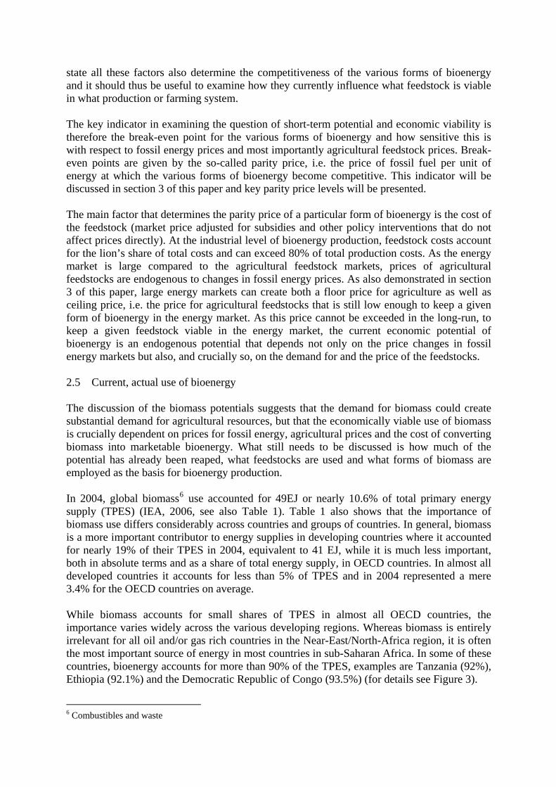
Crude oil prices drive sugar prices

0

10

20

30

40

50

60

70

80

90

31 January2000

31 January2001

31 January2002

31 January2003

31 January2004

31 January2005

31 January2006

31 January2007

US$

/bbl

0

2

4

6

8

10

12

14

16

18

20

Cts

/lb

West Texas Intermediate Rawsugar contract Nr 11, NYBOT

Figure 4: Sugar prices track crude oil price above US$35/bbl

Parity prices for sugar, Brazil, impact of carbon credits

0.00

5.00

10.00

15.00

20.00

25.00

20 30 40 50 60 70 80 90 100 110

US$/bbl WTI

raw

sug

ar, B

razi

l, ct

/lb

Cane-Braz, no CO2 bonus Cane-braz, CO2 bonus

Calculations based on data from a sugar mill + CHP plant in Santa Adelia, Brazil The unit produces 150000 t of raw sugar and about 100000 m3 ethanol.The project was awarded the title “Best CDM project 2004”, it has sold the CERs for electricity co-generation to a company in Europe. The CHP has a capacity of 100 MW, 65MW of which are fed into the local grid.

Figure 5: Parity prices for various first generation feedstocks

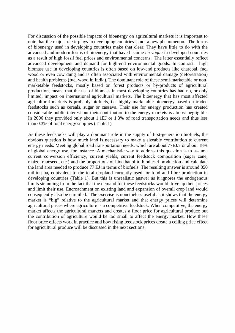
Figure 7: Parity prices (PP) for sugar and CDM effects on PPs Figure 6: Floor and ceiling price effect for Cassava, mega plant

... there is no complete market integration in practice ...

In practice, however, demand for biofuels is not driven by infinitely large demand. There are numerous constraints that limit the ability of the biofuel sector to reap the full demand potential, at least in the short run. For transportation fuels, availability for the final consumer and thus demand is circumscribed by bottlenecks in the distribution (lack of petrol stations), technical problems in transportation and blending systems (no pipeline transportation for ethanol due to corrosion problems), insufficient conversion capacities, delays in engine adjustments and development, and many more. In short, the entire “field-to-wheel” system is not yet fully developed for biofuels. For heating fuels, bottlenecks include logistical problems within households, lack of storage capacity given the much higher space requirements and the lower energy density of biofuels, unresolved emission problems (micro-particulates, NOx, CO, etc.), etc.

... except for cane-based ethanol in the Brazilian petrol market.

While most bioenergy markets are still in their infancy, there are a few that are already largely developed and integrated. The Brazilian sugar/ethanol market is probably the most developed and integrated as well as the most profitable one. Market integration is characterised by: (i) a high market penetration for cars that can run on ethanol or any blend of ethanol and petrol; (ii) a country-wide system of petrol stations that offer ethanol; (iii) a growing share of sugar mills that can flexibly switch between sugar and ethanol production; (iv) a small but also rising share of specialised ethanol plants; (v) high-tech conversion and energy production systems, e.g. an integrated energy production system with growing share of combine heat power plants and electricity co-generation.

The cumulative experience over the last 30 years of cane-based ethanol production has resulted in a sharp decline in production costs (see Goldemberg, et al 2004 for details). The integrated cane-based ethanol/electricity co-generation system in Brazil becomes a competitive energy provider at crude oil prices of about US$35/bbl. At this level, Brazilian sugar millers can produce ethanol cum electricity without subsidies. This also means that as of this threshold, prices for sugar should move in sync with petrol prices, and if markets are fully integrated, the co-movement of sugar and petrol prices should even hold for rather short-term changes. Figure 4 one depicts this co-movement of sugar and oil prices. It shows that (i): demand for ethanol has created a floor price for sugar at about US$35/bbl. Oil prices above US$35/bbl make cane-bioenergy (ethanol and electricity) competitive for the energy market and create a co-movement of energy and sugar prices. At (and above) this price level, a sugar/ethanol producer in Brazil will sell sugar only for a price that is at (and above) the energy price equivalent8. (ii) the co-movement of sugar and oil prices is strong, particularly over weeks and months but often even on a daily basis.

Higher use of cane for ethanol production reduces sugar availabilities for exports onto the world market (Figure A2) and these sugar exports in turn lift international sugar prices. The net result is a close link between energy prices (both for ethanol and crude oil) and sugar prices, i.e. that sugar prices closely track oil prices (Figure 4).

8 A price of US$35/bbl corresponds to about USc7/lb for raw sugar.

How does the energy-agriculture price transmission work in a fully integrated biofuel market?

Full flexibility on both the demand and the supply side ensure the tight price link in practice: On the demand side, the rapidly growing share of flex-fuel vehicles (FFVs)9 i.e. cars that can run on gasoline and any blend of hydrous or anhydrous ethanol up to 85 percent, allows consumers to shift almost instantaneously between the two energy alternatives (ethanol and petrol). By the end of 2005, almost 900,000 FFVs had already been sold. The share of these vehicles in new car registrations is expected to rise to 80% in 2006 and several car manufacturers have announced that in future they will only be producing FFVs (F.O. Licht, 2006). With the rapid increase in FFV sales, the share of ethanol in the Otto fuel market increased to 40% in by the end of 2005 (F.O. Licht, 2006). On the supply side, the growing share of sugar mills that can flexibly shift between sugar and ethanol allows producers to switch almost instantaneously between sugar and ethanol production10. As Brazil is not only the second-largest producer of sugar but also the by far the most important exporter, these shifts between sugar and ethanol determine the availability of sugar on the world markets and thus world market prices for sugar11. In short, the consumers ensure the link between oil and ethanol, the producers between ethanol and sugar prices; together they create a strong link between oil and sugar prices (Figure 4). (iii) However, the high and rising flexibility does not exclude that prices for sugar over or undershoot their energy parity price levels in the short run. But the high flexibility on both sides and an increasing awareness in the financial industry of the tight link ensures that the two prices move quickly back to the fundamental parity price relationships. Econometrically, this co-movement is corroborated when a co-integration regression (more precisely “threshold co-integration”) of the two series is undertaken. It can be shown that the price for sugar (Nymex, contract No 11) and oil (WTI, spot) are co-integrated with a threshold of about 35US$/bbl.

No other country and production system has a bioenergy market with the same level of market integration. There are, however, a number of markets where market integration and thus the price link has become increasingly tight. These include the wood pellets market and to a lesser extent the wood chips market in Austria, the prices for both have been following with a growing degree of correlation the prices for heating fuel in 2006 and 2007. A low level of market integration is not a phenomenon that is limited to the bioenergy segment of the energy markets. It also applies to the gas sector both vis-à-vis the oil market and for the gas market across continents. The lack of market integration between the European and the US gas market is largely a reflection of physical market separation, as gas can only be economically 9 The share of FFV in new car registrations in Brazil reached 34% in December 2005, (Sillas 2005) but increased to 80% by the end of 2006 (F.O. Licht). 10 There is full flexibility at the margin but not full flexibility for the average of cane processed by Brazil’s sugar mills. Most mills are able to make a maximum of about 55% of one product and 45% of the other. In the early weeks of a typical harvest and before the flow of cane has reached its peak, most mills tend to make more ethanol than sugar. “With alcohol stocks remaining low, the product is usually more attractive than sugar. The characteristics of cane which matures early in the harvest also make it more suitable for distilling into ethanol than refining into sugar. However, once harvesting has reached its mid-year peak and mills are working at full capacity, they have to make a similar amount of each product in order to keep pace with the flow of cane reaching them. It is only when the flow of cane slows towards the end of the harvest that mills can really choose whether to make more sugar or alcohol with relative prices and apparent prospects of each product at that time playing a key role” (F.O. Licht, 2006). 11 The close link between sugar prices and ethanol prices are corroborated by the strong correlation between Brazil’s sugar exports and ethanol prices.

shipped in liquid form. The growing importance of gas liquification and thus of improved transportation options is likely to bring these markets closer together and their price movements more into sync.

3.2 Fossil fuel prices also create a ceiling for agricultural prices

Energy prices not only can create a lower limit for agricultural prices, they can also create an upper boundary. In the long run, agricultural prices will not rise faster than energy prices. If they do, and irrespective of their doing so in the short run, agricultural feedstocks price themselves out of the energy market. Floor and ceiling prices together can thus create a price corridor for agricultural products, in which price fluctuations are (co-)determined by their energy equivalents and the current energy price. Figure 6 shows the ceiling price that can be paid by a cassava-based ethanol plant in Thailand. If cassava prices move above 1200 baht/t as they did in the late 1990s, only very high oil prices of US$70/bbl and above would keep cassava in the ethanol market. If cassava prices rise above this level, the feedstock loses its competitiveness in the bioenergy market, demand for it falls or ceases altogether and prices decline again. Figure 7 illustrates how additional payments/benefits (in this case through the “Clean Development Mechanism (CDM) of the Kyoto Protocol) can alter the parity price levels and affect the ceiling price effect.

The effect of a long-term price ceiling does not exclude short-term supply disruptions or speculative reasons creating short-term swings that exceed the parity price level. The very high sugar prices (which exceeded their parity price levels to oil by a margin of about 4ct/lb in late November 2006 are a case in point. The ceiling price effect has also become visible in other agricultural market. In Germany for instance, higher maize prices have made maize too expensive a feedstock for biogas production and resulted in lower demand and a situation where half of the plants are making losses on a total cost basis12. Similarly, lower oil prices and maize prices of US$4/bushel and more have squeezed the profit margins for maize-based ethanol production in the US which will, in the long-run, create a ceiling price somewhere in the vicinity of US$5/bushel. At these and higher price levels, particularly older ethanol plants should become unprofitable and this would – barring major subsidies – reduce maize demand and thus put a lid on maize price increases. Again, this does not mean that maize prices cannot increase further in the short run. Should, as some observers13 predict, US maize supplies become exhausted by June 2007, short-term price peaks of US$6-7/bushel are deemed possible. At these prices, however, a growing share of ethanol producers would not even meet variable costs14, thus cease production in the short-term and relieve upward price pressure in the US maize markets.

3.3 Price transmission from energy to agriculture: multiple channels and a growing number of agricultural markets/commodities

The price transmission from energy markets to agricultural markets takes place through a number of channels. First, there are direct, own price links on the supply side. When higher energy prices make an agricultural product competitive for the energy markets, the energy

12 Based on a presentation by Dr Broderson, Managing Director, DLG, at the DKB-Eliteforum Landwirtschaft 2006, Schloß Liebenberg, Germany, November 2006. 13 Randy Schnepf, Congressional Research Service of the US, Presentation at the SAF, SAF-agriculteurs de France, Prospective PAC Agro ressources et Politique agricole commune, 8 rue d’Athènes 75 009 PARIS, 15 March 2007. 14 The short-term production criterion.

market sucks up agricultural feedstock and thus raises feedstock prices. The link weakens again when demand has driven prices up to a point where agricultural feedstocks become too expensive as a source of energy for the energy market. Second, there is an indirect price transmission through substitutes on the supply side. Higher price for a given product (e.g. sugar) create increasing competition with other agricultural crops, thus reducing the availability of these products on the markets and driving up their prices. In addition, rising energy prices increase the number and the quantities of agricultural feedstocks that are competitive for bioenergy and can therefore no longer be supplied to food and feed markets. For instance, the use of cassava in Thailand for bioethanol production will reduce the availability of this product for exports and thus support cereal prices both in Thailand and, because of lower cassava exports, elsewhere. Likewise, the expansion of palm oil production in Malaysia has already created competition for other plantation crops and has reduced rubber and cocoa production. Third, there is price transmission through the demand side. Higher oil prices have already increased prices for nylon and other synthetic fibres and thus indirectly increased buttressed prices for cotton. Likewise, higher oil prices raise the prices for synthetic rubber and thus will increase the competitiveness of natural rubber. This provides room for natural rubber prices to rise.

3.4 Differential price impacts across agricultural markets

The co-movement of prices, however, is not a universal feature across all agricultural markets. Prices will neither increase unabatedly (open-ended) nor uniformly across all food products. The ceiling price effect discussed above is crucial for understanding why an increased bioenergy use is unlikely to create open-ended food price increases and thus a global, long-term food security problem. Importantly, and as demonstrated above, food prices cannot rise faster than energy prices simply because they would then lose their competitiveness in the energy market. The fact that there are different levels of competitiveness for individual feedstocks and that many feedstock contain both energy and protein means that the price effect will not be uniform. In the long-run and barring major policy distortions (subsidies, border measures, etc.), food products will only enter the bioenergy market if they are competitive feedstocks for conversion into fuel (heating or transportation). This means that feedstocks like sugar, cassava or palm oil could experience the strongest price rise, because they have the lowest break even points (Figure 5) and the highest level of competitiveness. The second reason for a non-uniform price increase is that the bioenergy demand is limited to the energy part of feedstocks and this selective demand creates a considerable amount of protein-rich by–products. This means that protein prices are likely to rise less rapidly than energy prices or could even fall in absolute terms. The importance of the selection of feedstocks and the impacts on energy versus protein prices is available from Table 1.

In general, prices for energy-rich crops (sugar, starch-rich crops or woody biomass) stand to benefit from the added energy demand, while those for protein-rich commodities and those for by-products of the bioenergy conversion process are likely to decline. Such negative price impacts have already been noticeable for some by-products such as glycerine, DDGS15, corn

15 The wet milling process renders for a tonne of maize used to produce ethanol a total of xx kg of CGM and xx kg of CGF. Alternatively, the dry milling renders 321 kg of Distillers Dried Grains Soluble (DDGS). CGM and CGF have a protein content of 60% and 21% respectively, and a protein content of about 75 MJ ME, i.e. somewhat less than maize but somewhat more that barley. DDGS on the other hand has a protein content of 27%, 11% fat and 9% fibre. In either case, these by-products are suitable substitutes for traditional protein-rich feedstuffs like soybean meal, even though their high phosphorous and crude fibre contents can put limits on their

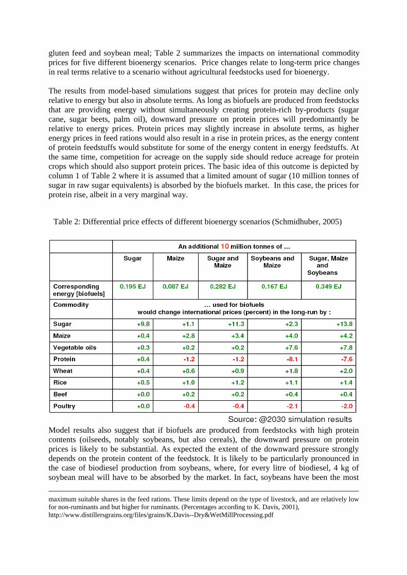
gluten feed and soybean meal; Table 2 summarizes the impacts on international commodity prices for five different bioenergy scenarios. Price changes relate to long-term price changes in real terms relative to a scenario without agricultural feedstocks used for bioenergy.

The results from model-based simulations suggest that prices for protein may decline only relative to energy but also in absolute terms. As long as biofuels are produced from feedstocks that are providing energy without simultaneously creating protein-rich by-products (sugar cane, sugar beets, palm oil), downward pressure on protein prices will predominantly be relative to energy prices. Protein prices may slightly increase in absolute terms, as higher energy prices in feed rations would also result in a rise in protein prices, as the energy content of protein feedstuffs would substitute for some of the energy content in energy feedstuffs. At the same time, competition for acreage on the supply side should reduce acreage for protein crops which should also support protein prices. The basic idea of this outcome is depicted by column 1 of Table 2 where it is assumed that a limited amount of sugar (10 million tonnes of sugar in raw sugar equivalents) is absorbed by the biofuels market. In this case, the prices for protein rise, albeit in a very marginal way.

Table 2: Differential price effects of different bioenergy scenarios (Schmidhuber, 2005)

Model results also suggest that if biofuels are produced from feedstocks with high protein contents (oilseeds, notably soybeans, but also cereals), the downward pressure on protein prices is likely to be substantial. As expected the extent of the downward pressure strongly depends on the protein content of the feedstock. It is likely to be particularly pronounced in the case of biodiesel production from soybeans, where, for every litre of biodiesel, 4 kg of soybean meal will have to be absorbed by the market. In fact, soybeans have been the most maximum suitable shares in the feed rations. These limits depend on the type of livestock, and are relatively low for non-ruminants and but higher for ruminants. (Percentages according to K. Davis, 2001), http://www.distillersgrains.org/files/grains/K.Davis--Dry&WetMillProcessing.pdf

important feedstock for biodiesel in the US. The results model simulations in Table xx suggest that the price effect can be noticeable. For every additional 10 million tonnes of soybeans combined with every extra 10 million tonnes of Maize, protein prices would fall be 8%. Also derived products which require large quantities of protein feed such as poultry meat would experience a mild downward pressure on prices (2%).

There are, however, reasons to assume that this downward pressure on protein prices as well as the upward pressure on energy prices are unlikely to increase proportionally with higher quantities of the feedstocks used for bioenergy. For one, protein feedstuffs for animal feed rations also contain energy and the cheaper energy in the feed proteins will start to replace the energy from the increasingly expensive energy feedstuffs (within the relevant physiological limits). This effect has already been noted within the current, first generation use of bioenergy crops. For another, a growing shift towards the second generation bioenergy feedstocks will further strengthen the co-movement in protein and energy prices. The application of second- generation bioenergy technologies means that the entire crop will be used to produce bioenergy, in contrast with the present practice of utilizing only a (potentially small) part of the feedstock (energy) while the protein-rich rest is returned to agricultural markets. Both, the feed effect as well as the shift towards second-generation bioenergy technologies will stop protein prices from falling and energy prices from rising so that they move again in sync (Schmidhuber, 2005).

The third factor that can have an important effect on relative prices can emerge from support and protection policies. Subsidies and tariffs are important reasons today why cereals are used in the US and in Europe as feedstocks in the bioethanol industries of these countries (some of the most important trade barriers are illustrated in Figure A4, Annex). Whether protection and subsidies could be justified on grounds of energy security, infant industry protection, or environmental benefits is a debatable issue. For the analysis of price effects on agricultural markets it should suffice to note that these tariffs keep prices for feedstocks higher than they would otherwise be and thus increase, directly or indirectly, prices for food with consequent effects on food security. The next and final section of this paper will examine how the price effects (floor price effect, ceiling price effect and differential price changes) discussed in section 4 could affect food security. The price impacts on the various dimensions of food security, i.e. food availability, access to food, food utilization and stability will be discussed separately.

4 Impacts on food security

The FAO defines food security as a “situation that exists when all people, at all times, have physical, social and economic access to sufficient, safe and nutritious food that meets their dietary needs and food preferences for an active and healthy life” (FAO, 2002a). This definition comprises four key dimensions of food supplies: availability, stability, access and utilization. The first dimension relates to the availability of sufficient food, i.e. to the overall ability of the agricultural system to meet food demand. Its sub-dimensions include the agro-ecological fundamentals of crop and livestock production, as well as the entire range of socio-economic and cultural factors that determine where and how farmers perform in response to markets. The second dimension, stability, relates to individuals who are at high risk of temporarily or permanently losing their access to the resources needed to consume adequate food. This is either because these individuals cannot insure ex ante against income shocks or

because they lack enough “reserves” to smooth consumption ex post or both. The third dimension, access, covers access by individuals to adequate resources (entitlements) to acquire appropriate foods for a nutritious diet. Entitlements are defined as the set of all those commodity bundles over which a person can establish command given the legal, political, economic and social arrangements of the community of which he or she is a member. Thus a key element is the purchasing power of consumers and the evolution of real incomes and food prices (Schmidhuber and Tubiello, 2007). However, these resources need not be exclusively monetary but may also include traditional rights e.g. to a share of common resources. Finally, utilization encompasses all food safety and quality aspects of nutrition; its sub-dimensions are therefore related to health, including the sanitary conditions across the entire food chain. It is not enough that someone is getting what appears to be an adequate quantity of food if that person is unable to make use of the food because he or she is falling sick.

4.1 Access to food

Agriculture is not only a source of the commodity food but, equally importantly, also a source of income. In a world where trade is possible at reasonably low cost, the crucial issue for food security is not whether food is “available”, but whether the monetary and non-monetary resources at the disposal of the population are sufficient to allow everyone access to adequate quantities of food The key factors that affect changes in access to food are real incomes and real prices for food. A greater role of bioenergy has an effect on both.

Price effects: Higher prices will reduce the purchasing power of consumers with adverse effects on their food security. But as discussed prices will neither increase indefinitely nor uniformly across all food products. In the long-run, neither food energy nor protein prices can rise faster than fuel energy prices in order for these feedstocks to remain competitive in the fuel energy market. This means that a global long-term food security problem due to increased bioenergy use would only be credible when and if real energy prices continue to rise. And even if they did, it would only reduce access to food and increase food insecurity if real food prices rose faster than real incomes.

In the short-run and during first-generation bioenergy use, prices for energy will rise faster than prices for protein. In a food insecurity situation where protein rich feedstocks are in short supply, the extra amounts of protein at lower prices would attenuate the adverse impacts from higher food energy prices, and may even make food rations more nutritious and thus improve the quality of food. As discussed, generally lower protein prices would be the outcome of a bioenergy scenario that would be based on the use of protein-rich oilseeds such as soybeans or rapeseed perhaps combines with the use of cereals such as maize or wheat as feedstocks for ethanol production. As also discussed, while these feedstocks indeed play an important role today, their low energy efficiency and their low carbon sequestration effects suggest that they will give way to more efficient converters of sunlight such as sugar cane or ligno-cellulosic feedstocks such as straw, miscanthus, poplar, or willow. In the long-run, it is also unlikely that the wedge between protein and energy prices will continue to increase.16

Income effects: An increased use of bioenergy is likely to affect not only prices and price patterns but also levels and the distribution of incomes, particularly in developing countries. For farmers, bioenergy should boost their overall revenues by raising both the prices they

16 For the interpretation of these price effects it is important to bear in mind that they reflect changes at the margin. Higher use may not simply have a proportionally higher price effect.

fetch for their products and the volume of products that they can sell on the markets. The price effect was discussed above. The positive volume effect is due to the fact that bioenergy makes certain farm products such as straw or crop residues -- for which there is currently no market other than bioenergy -- marketable products. A higher use of these products means that farmers may also face higher prices for some of their inputs and they may need to buy inputs like feedstuffs which where previously produced on the farm. In the long-run, they may also face higher wages if and where bioenergy boosts overall rural incomes. They may also face higher resource costs, notably higher land prices, as higher price for agriculture tend to capitalise on these scarce resources. Overall and notwithstanding the long-term adjustment processes in costs for land and labour, the positive revenue effect will exceed the costs and increase net farm incomes. Higher wages in rural areas and more employment effects should also increased overall rural incomes (trickle-down effect). The net effect on incomes in rural areas in general and in agricultural incomes in particular should thus be positive. And this also holds for access to food and food security in rural areas, and thus for 70 percent of all poor and undernourished, globally. The income effects of an increased use of bioenergy will also depend on the type of bioenergy with respect to factor demand. Where bioenergy is labour- intensive, factor incomes from cheap labour could help engender higher incomes for the poor. Conversely, where bioenergy is capital-intensive and labour-saving, impacts on incomes and thus access to food could be negative. Particularly hard hit will be land-less rural households that are both net buyers of both food and energy, particularly if they fail to benefit from the macro-economic benefits that bioenergy can bring about (higher employment rates and higher wages). The exact effects of course require further empirical analysis.

While many rural areas stand to benefit, urban households will face higher prices for food. Important here is to recall that food prices and energy prices rise in tandem and that the strength of the link between the two increases with rising energy prices. For net buyers of food and energy, this would be particularly negative. At the household level, a poor urban household with a high expenditure share on food and energy would be particularly hard-hit. What types of households stand to benefit or lose from the parallel increase of food and energy prices needs to be examined empirically. At the country level, a first empirical analysis has already been undertaken. The results are summarized in Figure 9a-d. These 4 charts show countries with less than US$5000 GDP per capita sorted in four rubrics according to their net trade positions for food and energy imports. The graphs illustrate the per capita net-trade positions in nominal US Dollars of 2004 at different levels of oil prices, ranging from US$30/bbl to US$60/bbl. The energy imports include all forms of energy (oil, coal, gas, electricity). For the price changes in the energy sector it is assumed that the non-oil forms of energy increase in sync with oil prices. The revenues from agricultural exports refer to all agricultural products; the price links are endogenous and model-based. The strength of the link increases in a more than linear manner. This is due to the fact that higher energy prices make a growing number of commodities competitive for the energy market, and thus lifts their price with energy prices. It the long-run, higher levels of energy prices will also provide incentives for bioenergy investments and thus lead to a higher degree of market integration. Another consequence will be a co-movement of energy and agricultural prices for more products and in a firmer manner for each product.

The results of the analysis make it possible to categorise countries in four principal rubrics. Importers of agriculture and energy, these countries are in a lose-lose situation as they face higher current account deficits from both product rubrics and the deficit is likely to accelerate with rising energy prices. As discussed below, within this lose-lose rubric, two cases are to be distinguished. First, countries which can pass on the higher import expenditures for food and

energy to value-added export products; and second countries which import food and energy without being able to pass the extra costs onto their export sectors. In contrast, the positive extremes are countries that are traditional net exporters of both food and energy; these countries stand to benefit from price increases of both product categories and the increases in total current account surpluses are more than linear relative to the increases in oil price. Indonesia or Malaysia fall into this win/win rubric. And finally there are countries that export either food or energy and they tend to win or lose depending on the relative size of the food or energy exports and imports. They are in the upper left and lower left quadrant and are characterised as win/lose or lose/win cases.

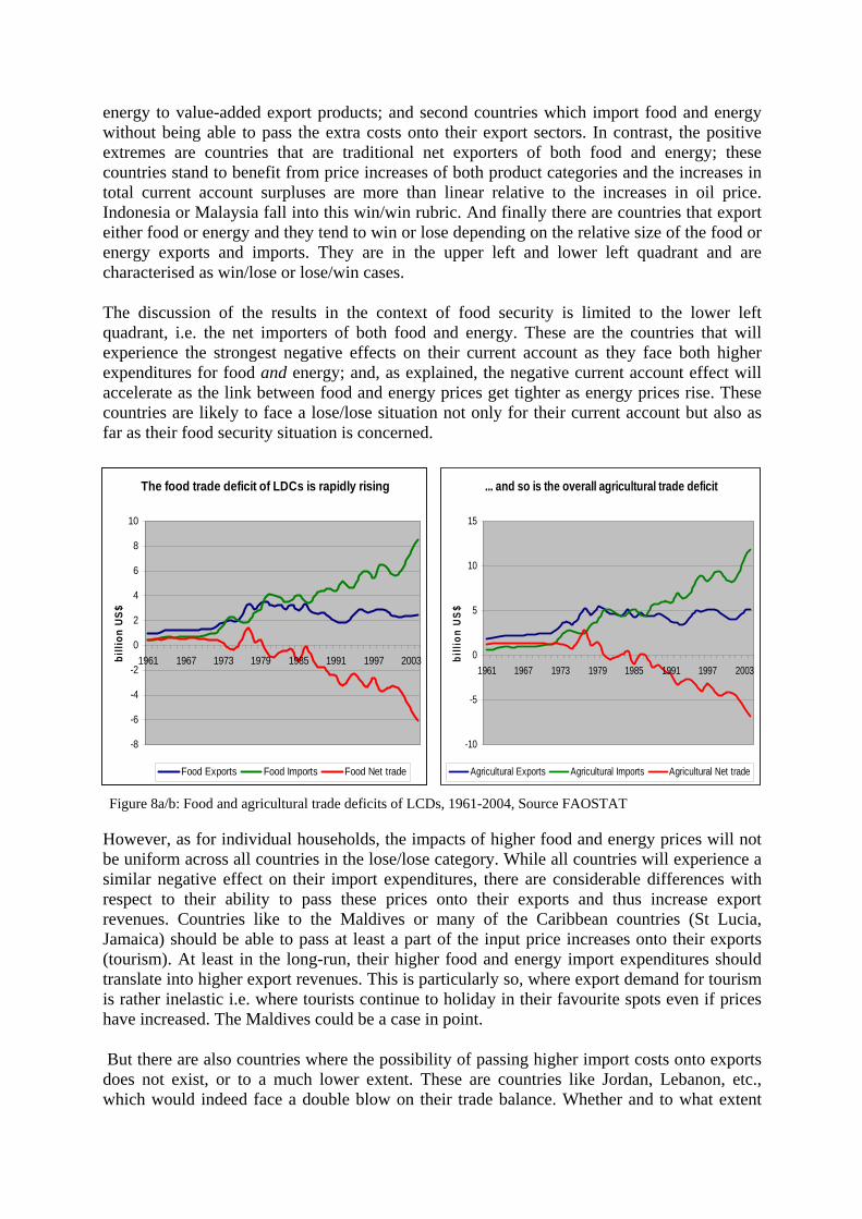
The discussion of the results in the context of food security is limited to the lower left quadrant, i.e. the net importers of both food and energy. These are the countries that will experience the strongest negative effects on their current account as they face both higher expenditures for food and energy; and, as explained, the negative current account effect will accelerate as the link between food and energy prices get tighter as energy prices rise. These countries are likely to face a lose/lose situation not only for their current account but also as far as their food security situation is concerned.

The food trade deficit of LDCs is rapidly rising

-8

-6

-4

-2

0

2

4

6

8

10

1961 1967 1973 1979 1985 1991 1997 2003billi

on U

S$

However, as for individual households, the impacts of higher food and energy prices will not be uniform across all countries in the lose/lose category. While all countries will experience a similar negative effect on their import expenditures, there are considerable differences with respect to their ability to pass these prices onto their exports and thus increase export revenues. Countries like to the Maldives or many of the Caribbean countries (St Lucia, Jamaica) should be able to pass at least a part of the input price increases onto their exports (tourism). At least in the long-run, their higher food and energy import expenditures should translate into higher export revenues. This is particularly so, where export demand for tourism is rather inelastic i.e. where tourists continue to holiday in their favourite spots even if prices have increased. The Maldives could be a case in point.

But there are also countries where the possibility of passing higher import costs onto exports does not exist, or to a much lower extent. These are countries like Jordan, Lebanon, etc., which would indeed face a double blow on their trade balance. Whether and to what extent

Food Exports Food Imports Food Net trade

... and so is the overall agricultural trade deficit

-10

-5

0

5

10

15

1961 1967 1973 1979 1985 1991 1997 2003

billi

on U

S$

Agricultural Exports Agricultural Imports Agricultural Net trade

Figure 8a/b: Food and agricultural trade deficits of LCDs, 1961-2004, Source FAOSTAT

this translates into a food security problem depends of course on the overall income levels in these countries. Overall, the poorest of the poor may be particularly hard hit. Most LDCs are both net importers of food (43 of 52 in 2002/04), net importers of agricultural products in general (38 of 52 in 2002/04) and overall they have considerable and rapidly growing multi-billion trade deficit for both food (US$6 billion) and agriculture (US$6.9 billion, see Figure 8a/b). As they are also the countries with the lowest level of GDP, the adverse effect from higher energy and agricultural imports relative to national incomes is likely to be particularly strong. How strong this effect is in practice will depend on the possibilities of individual countries to substitute for energy and agricultural imports or to pass higher import prices onto value-added exports.

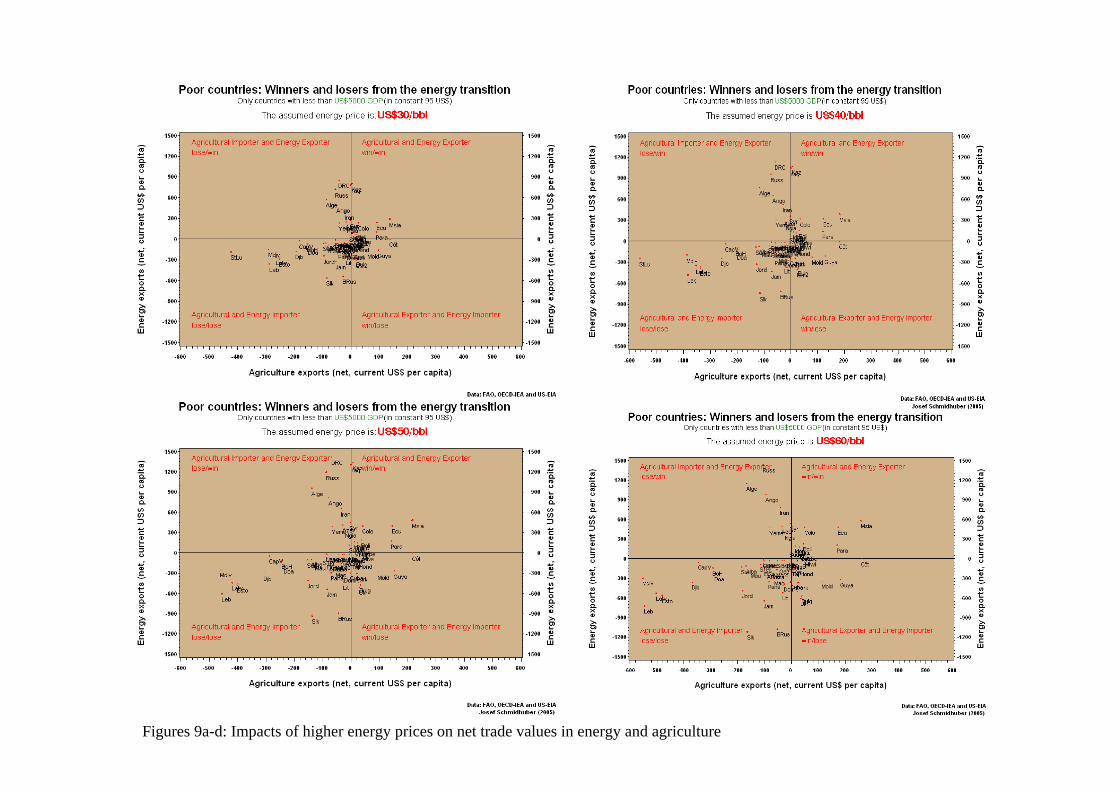
Figures 9a-d: Impacts of higher energy prices on net trade values in energy and agriculture

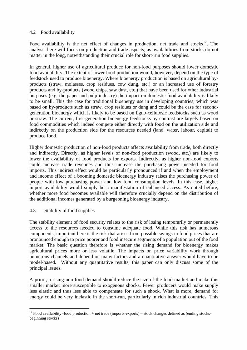
4.2 Food availability

Food availability is the net effect of changes in production, net trade and stocks17. The analysis here will focus on production and trade aspects, as availabilities from stocks do not matter in the long, notwithstanding their crucial role for short-run food supplies.

In general, higher use of agricultural produce for non-food purposes should lower domestic food availability. The extent of lower food production would, however, depend on the type of feedstock used to produce bioenergy. Where bioenergy production is based on agricultural by-products (straw, molasses, crop residues, cow dung, etc.) or an increased use of forestry products and by-products (wood chips, saw dust, etc.) that have been used for other industrial purposes (e.g. the paper and pulp industry) the impact on domestic food availability is likely to be small. This the case for traditional bioenergy use in developing countries, which was based on by-products such as straw, crop residues or dung and could be the case for second- generation bioenergy which is likely to be based on ligno-cellulosic feedstocks such as wood or straw. The current, first-generation bioenergy feedstocks by contrast are largely based on food commodities which indeed compete either directly with food on the utilization side and indirectly on the production side for the resources needed (land, water, labour, capital) to produce food.

Higher domestic production of non-food products affects availability from trade, both directly and indirectly. Directly, as higher levels of non-food production (wood, etc.) are likely to lower the availability of food products for exports. Indirectly, as higher non-food exports could increase trade revenues and thus increase the purchasing power needed for food imports. This indirect effect would be particularly pronounced if and when the employment and income effect of a booming domestic bioenergy industry raises the purchasing power of people with low purchasing power and low food consumption levels. In this case, higher import availability would simply be a manifestation of enhanced access. As noted before, whether more food becomes available will therefore crucially depend on the distribution of the additional incomes generated by a burgeoning bioenergy industry.

4.3 Stability of food supplies

The stability element of food security relates to the risk of losing temporarily or permanently access to the resources needed to consume adequate food. While this risk has numerous components, important here is the risk that arises from possible swings in food prices that are pronounced enough to price poorer and food insecure segments of a population out of the food market. The basic question therefore is whether the rising demand for bioenergy makes agricultural prices more or less volatile. The impacts on price variability work through numerous channels and depend on many factors and a quantitative answer would have to be model-based. Without any quantitative results, this paper can only discuss some of the principal issues.

A priori, a rising non-food demand should reduce the size of the food market and make this smaller market more susceptible to exogenous shocks. Fewer producers would make supply less elastic and thus less able to compensate for such a shock. What is more, demand for energy could be very inelastic in the short-run, particularly in rich industrial countries. This

17 Food availability=food production + net trade (imports-exports) – stock changes defined as (ending stocks-beginning stocks)

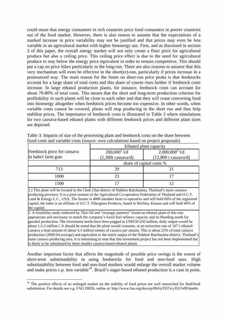
could mean that energy consumers in rich countries price food consumers in poorer countries out of the food market. However, there is also reason to assume that the expectations of a marked increase in price variability may not be justified and that prices may even be less variable in an agricultural market with higher bioenergy use. First, and as discussed in section 3 of this paper, the overall energy market will not only create a floor price for agricultural produce but also a ceiling price. This ceiling price effect is due to the need for agricultural produce to stay below the energy price equivalent in order to remain competitive. This should put a cap on price hikes particularly in the long-run. There are also reasons to assume that this very mechanism will even be effective in the short(er)-run, particularly if prices increase in a pronounced way. The main reason for the limits on short-run price peaks is that feedstocks account for a large share of total costs and this share of course rises further if feedstock costs increase. In large ethanol production plants, for instance, feedstock costs can account for about 70-80% of total costs. This means that the short and long-term production criterion for profitability in such plants will be close to each other and that they will cease converting food into bioenergy altogether when feedstock prices become too expensive. In other words, when variable costs cannot be covered, plants will stop producing in the short run and thus help stabilise prices. The importance of feedstock costs is illustrated in Table 3 where simulations for two cassava-based ethanol plants with different feedstock prices and different plant sizes are depicted.

Table 3: Impacts of size of the processing plant and feedstock costs on the share between fixed costs and variable costs (source: own calculations based on project proposals)

Ethanol plant capacity Feedstock price for cassava In baht/t farm gate

200,0001 l/d (1,300t cassava/d)

2,000,0002 l/d (12,800 t cassava/d)

share of capital costs % 713 29 21 1000 23 17 1500 17 12

1.) This plant will be located in the Chok Chai district of Nakhon Ratchasima, Thailand’s main cassava-producing province. It is a joint venture of the Agricultural Co-operative Federation of Thailand and O.C.T. Land & Energy L.C., USA. The former is 4000 member farm co-operative and will hold 60% of the registered capital, the latter is an affiliate of O.C.T. Fiberglass Products, based in Wichita, Kansas and will hold 40% of the capital. 2. A feasibility study endorsed by Thai Oil and “strategic partners” found an ethanol plant of this size appropriate and necessary to match the company’s fossil fuel refinery capacity and its blending needs for gasohol production. The investment needs have been pegged at US$150-250 million, daily output would be about 1.5-2 million l. It should be noted that the plant would consume, at an extraction rate of 167 l ethanol/ cassava a total amount of about 4.3 million tonnes of cassava per annum. This is about 25% of total cassava production (2000-04 average) and equivalent to the entire output of the Nakhon Ratchasima district, Thailand’s main cassava producing area. It is interesting to note that this investment project has not been implemented but is likely to be substituted by three smaller cassava-based ethanol plants.

Another important factor that affects the magnitude of possible price swings is the extent of short-term substitutability in using feedstocks for food and non-food uses. High substitutability between food and non-food markets would enlarge the overall market volume and make prices c.p. less variable18. Brazil’s sugar-based ethanol production is a case in point.

18 The positive effects of an enlarged market on the stability of food prices are well researched for feed/food substitution. For details see e.g. FAO 2002b, online at: http://www.fao.org/docrep/004/y3557e/y3557e09.htm#o

Given the high market integration of this market and its significant size both in domestic energy and international sugar markets, the non-food use of sugar works like a giant buffer stock for the sugar market that releases sugar on the market when it becomes too expensive for ethanol production and sucks it up when sugar is too cheap and it is more profitable to produce bioenergy out of the same feedstock. It can already be shown that not only the price levels of sugar but also the variability of the sugar prices follows closely the variability of energy prices; with the growing integration of the sugar-ethanol market, magnitude and frequency of sugar price variations closely trace those in crude oil.

The high degree of integration in the sugar market is however not (yet) characteristic of other agricultural feedstock markets. In most bioenergy markets substitutability is still low and rising utilization of agricultural feedstocks for bioenergy eats into the volumes of the corresponding food markets. This is particularly the case for many perennial crops (miscanthus, poplar, willow, etc.) where the limited or completely missing substitutability in conjunction with a multi-year area allocation to non-food production makes it more difficult to shift from non-food use to food use and vice versa. A massive shift towards such feedstocks may make overall food markets more susceptible to price shocks.

The discussion of the impacts of an increased bioenergy use shows that higher agricultural and energy prices can provide both a threat to but also an important opportunity for improving food security. At the country level, the short-term static effects of the likely price changes for food and energy will crucially depend on the net trade position for these products and the ability of a country to pass on higher import prices to higher export values for derived products. Similarly, the effects at the individual household level will depend on whether a household is a net buyer of these products. In general, it can be expected that individual households will either be in lose/lose or in a win/win situation. In general, rural households stand to benefit from both higher food prices and higher volumes of marketable produce which they can sell as bioenergy feedstocks. Urban households stand to lose as net buyers of both food and energy.

Policies can play an important role in mitigating the adverse effects on net buyers of food and energy and ensure that net sellers of both are able to fully harness the benefits. If and where the right policies are in place, the use and production of bioenergy affords rural areas the chance of a renaissance. It could help attract resources back into the countryside, mitigate urbanisation pressures and initiate a new rural dawn. But a lot more work is needed to analyse the appropriate companion policies in order to maximise the benefits for rural areas without causing massive problems for urban dwellers.

Summary, conclusions and outlook

The paper illustrated energy markets are affecting agricultural markets and showed how. It briefly introduced nature and size of bioenergy potentials, examined price and market effects and discussed possible impacts on food security. The key findings and the main conclusions that follow from these findings can be summarized as follows:

1. Rising prices for fossil energy have made a growing number of agricultural feedstocks competitive feedstocks for the energy market. The extra demand has resulted in a global increase in agricultural commodity prices and the creation of a floor price effect for competitive feedstocks. The potential demand from the overall energy market is so large that it could result in a change in the overall paradigm of rapidly rising supply, increasingly saturated demand and falling real prices that has governed international agricultural markets over the last 40 years.

2. Higher real prices in agriculture will have numerous effects on rural areas, rural industries and food security. They create opportunities but also new challenges. Higher real prices can help revitalise rural areas and help reduce rural poverty. The combination of higher prices and more marketable produce will raise overall revenues for agricultural households. In tandem, rural, non-agricultural households could benefit from new employment opportunities and higher wages and thus higher incomes. The positive income effect should be particularly pronounced where bioenergy production and processing is labour-intensive and access to land is relatively equitable. Overall, the effect could be a global renaissance of agriculture and a revitalisation of rural areas.

3. A new bust after the first generation boom? While bioenergy has the potential to arrest the long-term downward trend in real prices for food and agriculture, the effect may be limited in time and size and even a longer interruption in falling real prices may not mean a complete and permanent departure from the century-long downward trend. Episodes of rising real prices are not new and the long-term price decline over the last century was characterised by three periods or rising real prices (1900-18, 1933-48, 1973-80, 2000-2007). These periods lasted more than a decade and they were typically followed by pronounced bust cycles. High-price periods have led farmers to expand and intensify production, invest in land and technology and assume debt to an extent that has later proven unsustainable. What is more, much of the increased price was typically capitalized in the price of land rather than resulting in the longer-term profitability of farm operations. Higher values of collaterals, high short-term profitability followed by pronounced bust cycles led to large amounts of non-performing loans in agriculture and periods of widespread financial distress in farming. The US "farm crisis" of the 1980s is the most recent example (Gardner, 2003).

4. The current bioenergy-triggered boom could also be followed by a marked bust cycle. It could be ushered when the second generation biotech feedstocks enters the market on a large scale. Second-generation technologies could make many of the first generation feedstocks (i.e. the traditional agricultural and food commodities) unprofitable and result in a demand and price shift from food commodities to forests commodities. This shift could make not only first-generation feedstock production unprofitable, but the entire production chain as well because second-generation processing technologies will be entirely different. For food prices, this should result in less demand and possibly a return to falling real prices.

5. New support and protection policies in developed and developing countries for bioenergy, combined with new policy initiatives (CDM, JI, GEF, etc.) at the international level and a growing engagement by International Financial Institutions could add to possible over-

investments in bioenergy production. The simultaneous commitment to investing in the same sector could result in a global “fallacy of composition” problem. As more efficient first-generation plants come on stream and as second-generation technologies enter the bioenergy markets, a lot of investments in first-generation bioenergy could turn sour or remain only profitable if real prices for fossil energy remain high and rising. The first signs of such problems are already visible in the low profitability of maize-based biogas production in Germany and of maize ethanol plants in the US given currently rising maize prices.

6. The growing dependence of agricultural prices on energy prices also means that there will be an endogenous cap on food price increases. In order to remain competitive for the energy market, agricultural feedstock prices cannot rise faster than energy prices in order to remain competitive as a source of energy. This creates an implicit ceiling price effect, which is given by the energy equivalent of an agricultural feedstock. The ceiling price effect is crucial for understanding that agricultural prices and markets will not continue the recent boom sparked by the spike in oil prices but also to understand that concerns about a looming global neo-Malthusian scenario are unwarranted19. Only if energy prices continue to rise will agricultural prices follow. Overall, floor and ceiling price effects are creating a new equilibrium for an increasing number of agricultural commodity markets. With rising energy prices and a growing degree of market integration between energy and agricultural feedstock markets, both the levels and variability of agricultural commodities will increasingly be determined by those of energy prices.

7. The impact on food security needs to be analysed in the context not only of higher food prices and lower availability but also in terms of rising incomes for farmers and rural areas as well as changing price variability. A priori, competition with food production will result in lower availability and an increase in food expenditures for the poor. Particularly net buyers of both food and energy would suffer from the parallel increase in food and energy prices. As net buyers of food and energy, the poorest of the poor could be particularly hard hit. At the country level, many developing economies are currently facing a double burden on their current account balance through higher expenditures for food and energy imports. The same holds for individual households that are both net buyers of food and energy. However, many rural households stand to benefit both through higher prices for their produce and higher volumes of marketable production. As 70 percent of the poor live in rural areas, the overall net effect on food security could be positive. While rural households stand to benefit as sellers of food and energy, urban households stand to suffer from higher expenditures for both. Importantly, food expenditures rises more than linearly as the price link between energy and food prices tightens with rising energy prices. While the inter-country effects have been quantified for this paper, the intra-country effects would need to be gauged by a detailed analysis of household balance sheet effects.

8. One of the challenges for the orientation of development policy is to design and implement policy measures that help ensure that the growing use of bioenergy is conducive to reducing poverty and hunger, i.e. that “bioenergy becomes pro-poor”; in theory, this will the case, the closer the factor demand of bioenergy is complementary to the factor endowment of the poor; in general this is the case when bioenergy use and processing are labour- intensive, capital-saving, and technology-saving. Pro-poor policies would help to adapt bioenergy use and processing accordingly so that they are based on

19 The predictions of a massive dooms day scenario caused by an increase of use of agricultural commodities for biofuel are numerous and massive. For instance, BBC International quotes the Cuban Fidel Castro of claiming that the US ethanol programme alone will cause 3 billion deaths from hunger, i.e. half the world’s population. http://news.bbc.co.uk/2/hi/americas/6505881.stm

little capital and simple technologies and abundant low-skilled labour. Pro-poor policies will also promote and foster access to technology and capital (e.g. through the CDM and CDM like mechanisms), provide access to land (land reform, etc.).

9. Functioning institutions that make an important contribution to making bioenergy pro-poor. Co-operatives for instance can bundle the interests of the poor, accumulate and attract capital for the necessary investments, organise feedstock supplies in large quantities and qualities and create a countervailing power to the high power concentration of firms operating in the energy market. While this paper did not explicitly discuss options, some of the examples used to assess the profitability of such co-operative operations have been presented (see e.g. Cassava-based ethanol production in the Chok Chai district of Nakhon Ratchasima).

10. FAO and other international organizations have an important role to play in providing information and analyses that help create the basis for investments in bioenergy in developing countries. They may also have an even more important role in ensuring that the policy distortions of developed countries agricultural markets’, which were slowly and painfully reduced in the 1990s, will not be re-introduced through the “bioenergy backdoor”. Failure here would not only impede the development of the bioenergy income potentials in developing countries but also compound and prolong a possible bust period after the current boom cycle. A simple first step to level the bioenergy playing field would be a noticeable reduction in tariffs for biofuels in developed countries, noticeable for bioethanol. As depicted in Figure A4 (Annex), these entry hurdles in developed countries can be considerable.

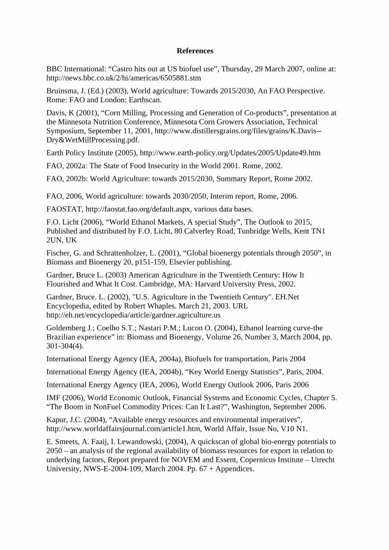
References

BBC International: “Castro hits out at US biofuel use”, Thursday, 29 March 2007, online at: http://news.bbc.co.uk/2/hi/americas/6505881.stm

Bruinsma, J. (Ed.) (2003), World agriculture: Towards 2015/2030, An FAO Perspective. Rome: FAO and London: Earthscan.

Davis, K (2001), “Corn Milling, Processing and Generation of Co-products”, presentation at the Minnesota Nutrition Conference, Minnesota Corn Growers Association, Technical Symposium, September 11, 2001, http://www.distillersgrains.org/files/grains/K.Davis--Dry&WetMillProcessing.pdf.

Earth Policy Institute (2005), http://www.earth-policy.org/Updates/2005/Update49.htm

FAO, 2002a: The State of Food Insecurity in the World 2001. Rome, 2002.

FAO, 2002b: World Agriculture: towards 2015/2030, Summary Report, Rome 2002.

FAO, 2006, World agriculture: towards 2030/2050, Interim report, Rome, 2006.

FAOSTAT, http://faostat.fao.org/default.aspx, various data bases.

F.O. Licht (2006), “World Ethanol Markets, A special Study”, The Outlook to 2015, Published and distributed by F.O. Licht, 80 Calverley Road, Tunbridge Wells, Kent TN1 2UN, UK

Fischer, G. and Schrattenholzer, L. (2001), “Global bioenergy potentials through 2050”, in Biomass and Bioenergy 20, p151-159, Elsevier publishing.

Gardner, Bruce L. (2003) American Agriculture in the Twentieth Century: How It Flourished and What It Cost. Cambridge, MA: Harvard University Press, 2002.

Gardner, Bruce. L. (2002), "U.S. Agriculture in the Twentieth Century". EH.Net Encyclopedia, edited by Robert Whaples. March 21, 2003. URL http://eh.net/encyclopedia/article/gardner.agriculture.us

Goldemberg J.; Coelho S.T.; Nastari P.M.; Lucon O. (2004), Ethanol learning curve-the Brazilian experience” in: Biomass and Bioenergy, Volume 26, Number 3, March 2004, pp. 301-304(4).

International Energy Agency (IEA, 2004a), Biofuels for transportation, Paris 2004

International Energy Agency (IEA, 2004b), “Key World Energy Statistics”, Paris, 2004.

International Energy Agency (IEA, 2006), World Energy Outlook 2006, Paris 2006

IMF (2006), World Economic Outlook, Financial Systems and Economic Cycles, Chapter 5. “The Boom in NonFuel Commodity Prices: Can It Last?”, Washington, September 2006.

Kapur, J.C. (2004), “Available energy resources and environmental imperatives”, http://www.worldaffairsjournal.com/article1.htm, World Affair, Issue No, V10 N1.

E. Smeets, A. Faaij, I. Lewandowski, (2004), A quickscan of global bio-energy potentials to 2050 – an analysis of the regional availability of biomass resources for export in relation to underlying factors, Report prepared for NOVEM and Essent, Copernicus Institute – Utrecht University, NWS-E-2004-109, March 2004. Pp. 67 + Appendices.

Schmidhuber, J and P. Shetty (2005), The nutrition transition to 2030. Why developing countries are likely to bear the major burden”, Acta Agriculturae Scand Section C, 2005; 2: 150-166.

Schmidhuber, J. (2005), “The nutrition and the energy transition of world agricultural markets”, Plenary presentation at the German Association of Agricultural Economists (GEWISOLA), Göttingen, October 2005.

Schmidhuber, J. (2006) Die Auswirkungen der Biomassenutzung auf die Weltagrarmärkte“ Kurzfassung des Vortrages zum Fachsymposium zu den „Perspektiven der energetischen Biomassenutzung“ Bad Hersfeld, 21. März 2006

Schmidhuber, J. and F.N. Tubiello (2007), “Climate Change and Global Food Security: Socio-economic dimensions of vulnerability”, paper accepted for publication in the Proceedings of the National Academy of Sciences (PNAS), 2007.

Sillas Oliva Filho (2005) The use of Ethanol in Brazil” Presentation at the UN World Environment day, San Francisco 2005.

World Bank (various issues), “Pink Sheets” World Bank Price Indicators, online available at: http://web.worldbank.org/WBSITE/EXTERNAL/EXTDEC/EXTDECPROSPECTS/0,,contentMDK:20268484~menuPK:556802~pagePK:64165401~piPK:64165026~theSitePK:476883,00.html.

World Bank (2004), World Development Indicators. CD-ROM.

Abbreviations

1. Units bbl Barrel, 159 litre

bushel (maize) 25.4012 kg

EJ Exajoule, 1018 joule

Mtoe (million tonne oil equivalent) = 41.868 PJ

PJ Petajoule, 1015 joule

2. Organizations FAO Food and Agriculture Organization of the United Nations

IEA International Energy Agency

IIASA International Institute for Applied Systems Analysis

NYMEX New York Mercantile Exchange

OECD Organization for Economic Co-operation and Development

USDA United States Department of Agriculture

3. Technical Terms

CO Carbon Monoxide

BTL Biomass to liquid

Fischer Tropsch The Fischer-Tropsch process is a catalyzed chemical reaction in which carbon monoxide and hydrogen are converted into liquid hydrocarbons of various forms.

LDC Least Developed Country

NOx Nitrogen oxide

TPES Total Primary Energy Supply

WTI West Texas Intermediate

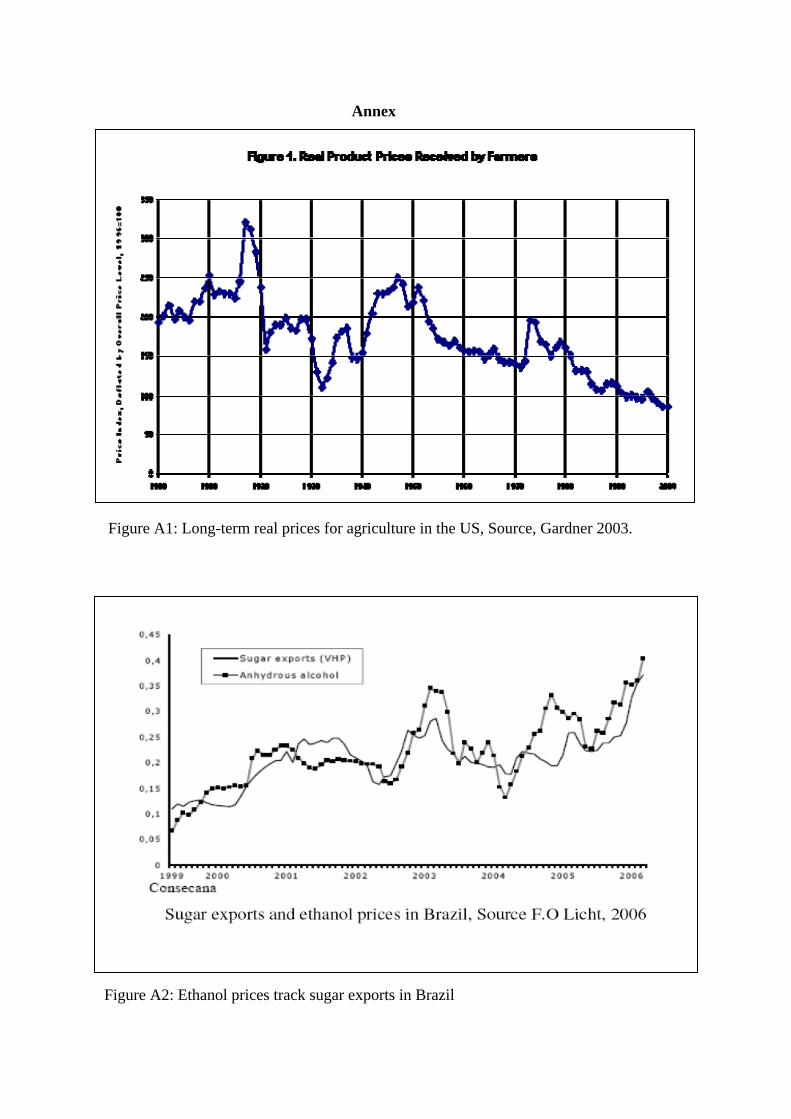
Annex

Figure A1: Long-term real prices for agriculture in the US, Source, Gardner 2003.

Figure A2: Ethanol prices track sugar exports in Brazil

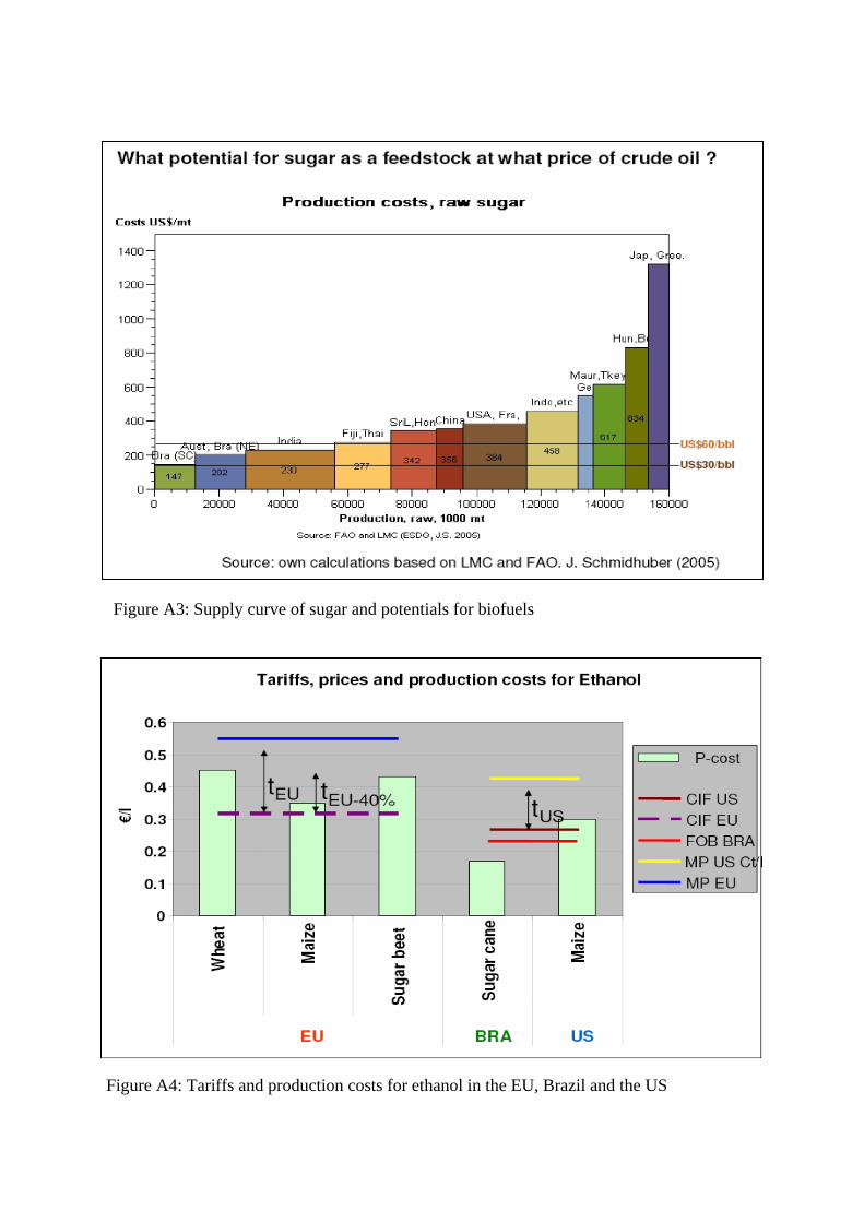
Figure A3: Supply curve of sugar and potentials for biofuels

Figure A4: Tariffs and production costs for ethanol in the EU, Brazil and the US