Impact of Atmosphere–Ocean Coupling on the Predictability

Impact of Atmosphere–Ocean Coupling on the Predictability of MonsoonIntraseasonal Oscillations*

XIOUHUA FU

IPRC, SOEST, University of Hawaii at Manoa, Honolulu, Hawaii

BIN WANG

IPRC, and Department of Meteorology, SOEST, University of Hawaii at Manoa, Honolulu, Hawaii

DUANE E. WALISER

JPL, California Institute of Technology, Pasadena, California

LI TAO

IPRC, SOEST, University of Hawaii at Manoa, Honolulu, Hawaii

(Manuscript received 25 July 2005, in final form 19 April 2006)

ABSTRACT

The impact of air–sea coupling on the predictability of monsoon intraseasonal oscillations (MISO) hasbeen investigated with an atmosphere–ocean coupled model and its atmospheric component. From a 15-yrcoupled control run, 20 MISO events are selected. A series of twin perturbation experiments have beenconducted for all the selected events using both the coupled model and the atmosphere-only model. Twocomplementary measures are used to quantify the MISO predictability: (i) the ratio of signal-to-forecasterror and (ii) the spatial anomaly correlation coefficient (ACC).

In the coupled model, the MISO predictability is generally higher over the Indian sector than that overthe western Pacific with a maximum of 35 days in the eastern equatorial Indian Ocean. Air–sea couplingsignificantly improves the predictability in almost the entire Asian–western Pacific region. The meanpredictability of the MISO-related rainfall over its active area (10°S–30°N, 60°–160°E) reaches about 24days in the coupled model and is about 17 days in the atmosphere-only model. This result suggests thatincluding an interactive ocean allows the MISO predictability of an atmosphere-only model to be extendedby about a week. The extended predictability is primarily due to the coupled model capturing the two-wayinteractions between the MISO and underlying sea surface. The MISO forces a coherent intraseasonal SSTresponse in underlying ocean that in return exerts an external control on the future evolutions of the MISO.

The break phase of the MISO is more predictable than the active phase in both the atmosphere-onlymodel and the coupled model as revealed in the observations. Air–sea coupling appears to extend the MISOpredictability uniformly regardless of the active or break phases.

1. Introduction

Intraseasonal variability is a dominant mode of theAsian–western Pacific summer monsoon (Yasunari

1980; Lau and Chan 1986; Wang and Rui 1990; Waliseret al. 2003b). This monsoon intraseasonal oscillation(MISO) constantly regulates the onset (retreat) and ac-tive (break) phases of the summer monsoon, and thusstrongly influences the weather-sensitive socioeco-nomic activities (e.g., agriculture) in this area (Websteret al. 1998; Gadgil and Rao 2000). The Asian–westernPacific region is also one of the most vulnerable areasaround the world to the impacts of climate-relatednatural disasters. About 80% of these natural disastersare caused by extreme hydrometeorological events(e.g., flood, drought, etc.; IFRC 2000). These extremeevents are also modulated by intraseasonal variability

* School of Ocean and Earth Science and Technology Contri-bution Number 7004 and International Pacific Research CenterContribution Number 422.

Corresponding author address: Dr. Xiouhua (Joshua) Fu, IPRC,SOEST, University of Hawaii at Manoa, 1680 East West Road,401 POST Bldg., Honolulu, HI 96822.E-mail: [email protected]

JANUARY 2007 F U E T A L . 157

DOI: 10.1175/JAS3830.1

© 2007 American Meteorological Society

JAS3830

(Goswami and Ajayamohan 2001; Goswami et al. 2003;Jones et al. 2004). If we could provide useful forecast ofthis intraseasonal variability with lead times of severalweeks, it will help the managements of weather-sensitive socioeconomic activities and reduce the dam-age caused by extreme events. In this study, we willexplore the predictability of the MISO in a hybrid at-mosphere–ocean coupled model and assess the impactsof air–sea coupling on the MISO predictability.

In an intuitive sense, the predictability of a specificatmospheric phenomenon has to be proportional to itsown lifetime (Van den Dool and Saha 1990). The re-current nature of the MISO suggests that, in principle,the useful prediction skill of rainfall associated with theMISO could be exploited by various models for leadtimes of a month or longer. Some statistical predictivemodels of the Intraseasonal Oscillation (ISO) have in-dicated useful skill out to about 15–25-day lead time(Waliser et al. 1999a; Lo and Hendon 2000; Mo 2001;Goswami and Xavier 2003; and Webster and Hoyos2004). For dynamical models, the pioneer studies ofKrishnamurti et al. (1990, 1992) suggested that the use-ful forecast skill of the flow fields associated with theMISO could reach 20–30 days for a few special events.From the historical view in the progress of weatherforecast (Kalnay 2003), we learned that both statisticaland dynamical models significantly contribute to theimprovement of forecast. Dynamical models, on theother hand, show greater potential to be improved andoffer more opportunities to advance our understand-ings of the related physical processes.

Waliser et al. (2003b,c) first systematically examinedthe potential predictability of the ISO [both the MISOin boreal summer and Madden–Julian oscillation(MJO) in boreal winter] using the National Aeronau-tics and Space Administration (NASA) Goddard Labo-ratory for Atmospheres (GLA) AGCM with a series oftwin-perturbation experiments. An objective signal-to-error measure was used to quantify the predictability ofthe ISO. They concluded that the limit of predictabilityfor the model’s ISO extends out to about 25 days for200-hPa velocity potential and to about 15 days forrainfall. Recently, Liess et al. (2005) found that theupper limit of rainfall predictability associated with theMISO in the ECHAM5 AGCM could reach one monthin some specific regions over the Asian–western Pacificdomain. With the National Centers for EnvironmentalPrediction (NCEP) forecast model, Reichler and Roads(2005) found that the predictability of the 200-hPa ve-locity potential in the Tropics reaches about 4 weeks,but almost no predictability for model rainfall whensame measure is used. These studies tend to suggestthat the potential predictability of some dynamic fields

associated with the ISO in the state-of-the-art AGCMscould reach about one month. However, the predict-ability of the ISO-related rainfall is much shorter andvaries considerably among different models.

Further, in an operational setting, the potential pre-dictability of dynamical models will be shortened by theerrors existing in the initial and boundary conditionsand the weaknesses of models in representing the struc-tures, intensity, and propagation of the ISO (Chen andAlpert 1990; Lau and Chang 1992; Hendon et al. 2000;Seo et al. 2005). The predictive skill of the boreal winterISO in an old version (Hendon et al. 2000; Jones et al.2000) and a latest version (Seo et al. 2005) of the NCEPforecast model is only about 7–10 days for the relateddynamic fields when SSTs are fixed on climatology. Therelative short forecast skill is largely related to the mod-el’s deficiencies in maintaining the large-scale circula-tions and representing the propagations of the ISO.Apparently, in order to improve the prediction of theISO in dynamic models, we need to further improve themodel representations of the ISO and explore betterways to set up the initial and boundary conditions.

On intraseasonal time scale, in addition to the initialconditions (Krishnamurti et al. 1992), boundary condi-tions (e.g., the intraseasonally varying SSTs) probablyalso play very important role on the ISO prediction(Reichler and Roads 2005). However, in an operationalsetting, the intraseasonal SST fluctuations are notknown a priori. Thus, an atmosphere–ocean coupledmodel is needed to generate an interactive SST for theforecast system. In fact, most previous studies have sup-ported the notion that air–sea coupling can significantlyimprove the simulation of tropical ISO compared toatmosphere-only models (Flatau et al. 1997; Wang andXie 1998; Waliser et al. 1999b; Kemball-Cook et al.2002; Fu et al. 2003; Inness and Slingo 2003; Matthews2004; among others). The exception of Hendon (2000)is largely attributed to errors in the model’s mean stateand an associated failure of the model to simulate acorrect relationship between ISO-driven surface latentheat flux and rainfall anomalies. Based on the afore-mentioned findings, we will address the following ques-tion in this study: Could the predictability of tropicalISO in an atmosphere-only model be improved by in-cluding active air–sea coupling? We expect a positiveanswer to this question for two reasons. First, by im-proving the simulation of the basic ISO characteristics,namely those related to spatial structure and evolution,intensity, propagation speed, and seasonality. Second,the intraseasonal SST fluctuations lead the ISO-relatedconvection by about 10 days in both the coupled model(Fu et al. 2003; Zheng et al. 2004) and the observations

158 J O U R N A L O F T H E A T M O S P H E R I C S C I E N C E S VOLUME 64

(Arakawa and Kitoh 2004); this relationship is notpresent in the atmosphere-only model. In other words,the intraseasonal SST fluctuations in the coupled sys-tem may provide a memory to extend the predictabilityof the ISO. This hypothesis will be examined in thefollowing study.

In section 2, we introduce the hybrid atmosphere–ocean coupled model and briefly validate the simulatedMISO with the satellite observations from the TropicalRainfall Measuring Mission (TRMM) Microwave Im-ager (TMI). (TMI data are acquired from RemoteSensing Systems available online at http://www.ssmi.com/tmi/tmi_browse.html.)

Section 3 describes the framework to conduct theensemble experiments and the methods to quantify thepredictability of the MISO, which basically follow thoseused in Waliser et al. (2003b,c). Section 4 presents theMISO predictability in the coupled model and the por-tion contributed by air–sea coupling. Section 5 exam-ines the dependence of the MISO predictability on theactive and break phases. Section 6 discusses some issuesraised from current study. The last section summariesour major findings and identify several future researchdirections.

2. Model

a. Model description

The hybrid coupled atmosphere–ocean model com-bines the ECHAM4 atmospheric general circulationmodel (AGCM; Roeckner et al. 1996) and an interme-diate ocean model (Wang et al. 1995; Fu and Wang2001). The details of this hybrid coupled model and itssimulations of the tropical Asian–Pacific climate can befound in Fu and Wang (2004b) and X. Fu et al. (2006,unpublished manuscript; available at http://www.soest.hawaii.edu/�xfu/HcGCM.pdf). For the convenience ofreaders, a brief description of the coupled model isgiven in the following.

The atmospheric model is a T30 version of ECHAM4with horizontal resolution of about 3.75° and 19 verticallevels extending from the surface to 10 hPa. Its landsurface scheme is a modified bucket model with im-proved parameterization of rainfall runoff (Dumeniland Todini 1992). The cumulus parameterization is amodified version of the mass flux scheme developed byTiedtke (1989). The improved version replaces theoriginal moisture-convergence closure scheme withconvective available potential energy (CAPE) closure(Nordeng 1994). The radiation scheme is a modifiedversion of the European Centre for Medium-RangeWeather Forecasts (ECMWF) scheme. Two- and six-

band intervals are used in the solar and terrestrial partof the spectrum, respectively.

The ocean component of this hybrid-coupled modelis a tropical upper ocean model with intermediate com-plexity. It was originally developed by Wang et al.(1995) and later improved by Fu and Wang (2001). Theocean model comprises a mixed layer, in which the tem-perature and velocity are vertically uniform, and a ther-mocline layer in which temperature decreases linearlyfrom the mixed-layer base to the thermocline base.Both layers have variable depths. The deep ocean be-neath the thermocline base is motionless with a con-stant reference temperature. This ocean model com-bines the mixed-layer physics of Gaspar (1988) and theupper ocean dynamics of McCreary and Yu (1992). Itreasonably simulates the annual cycles of sea surfacetemperature, upper ocean currents, and mixed layerdepth in the tropical Pacific (Fu and Wang 2001).

The ECHAM4 AGCM was coupled with the inter-mediate ocean model in the tropical Indian and PacificOceans (30°S–30°N) without heat flux correction [ex-cept that the SSTs in the north–south open boundarieshave been relaxed to the observed climatologicmonthly mean as in Fu and Wang (2001)]. Outside thecoupling region, the underlying sea surface tempera-ture is specified as the climatological monthly meanSST from the Second Atmospheric Model Intercom-parison Project (AMIP II) experiment (Taylor et al.2000). In the tropical Indian and Pacific Oceans, atmo-spheric component exchanges information with oceancomponent once per day. The atmosphere providesdaily mean surface winds and heat fluxes to the oceanmodel. The latter provides daily mean SST back to theformer. Prior to carrying out the forecast experiments,a 21-yr coupled integration was conducted. The outputfrom the last 15-yr of integration will be referred to asthe control run.

b. The MISO simulated in the coupled model

This hybrid coupled atmosphere–ocean model rea-sonably simulates the climatology and interannual vari-ability in the tropical Asian–Pacific sector (X. Fu et al.2006, unpublished manuscript). It also shows reason-able skill to reproduce the major observational charac-teristics of the MISO in the Asian–western Pacific sec-tor, such as the location of major active centers, sea-sonal variations in amplitude, dominant periods andspatial–temporal evolutions. Those characteristics havebeen validated in our previous studies (Fu et al. 2003;Fu and Wang 2004a,b; X. Fu et al. 2006, unpublishedmanuscript).

Figure 1 further compares the regressed rainfall andSST fluctuations associated with the MISO in the TMI


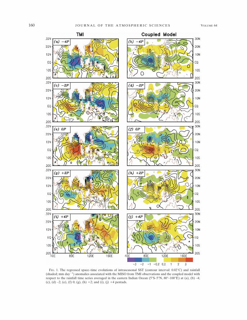
FIG. 1. The regressed space–time evolutions of intraseasonal SST (contour interval: 0.02°C) and rainfall(shaded; mm day�1) anomalies associated with the MISO from TMI observations and the coupled model withrespect to the rainfall time series averaged in the eastern Indian Ocean (5°S–5°N, 80°–100°E) at (a), (b) –4;(c), (d) –2; (e), (f) 0; (g), (h) �2; and (i), (j) �4 pentads.


Fig 1 live 4/C

observations (1998–2003) and the coupled model. Thefiltered rainfall (only 20–90-day variability is retained)over the eastern equatorial Indian Ocean (EIO; 5°S–5°N, 80°–100°E) is used as the reference time series forthe regression. At 4 pentads before the rainfall peaks inthe EIO (Figs. 1a,b), the dry phase prevails in the entireequatorial Indian Ocean and Maritime Continent witha rainy belt around 15°N in both the observations andthe coupled model. The positive SST anomalies start toform in the equatorial Indian Ocean associated withreduced convection. The negative SST anomalies, ow-ing to enhanced convection, appear in the northern sideof the dry zone. Both the internal dynamics (Jiang et al.2004) and SST anomalies (Fu et al. 2003) play a role inleading to the disturbances moving northeastward(Figs. 1c,d). When the dry zones move off the equator,the MISO-related convection initiates and intensifies inthe equatorial Indian Ocean (Fig. 1c–f). The positiveSST anomalies start to form in the northeast side of thewet zone and help the convection moving northeast-ward (Figs. 1g–j). The simulated rain-belt in the north-ern Indian Ocean (Fig. 1h) is weaker and moves slowerthan the observed (Fig. 1g).

Overall, the patterns of rainfall and SST anomaliesbetween the observations and the simulations are simi-lar except that the magnitude of rainfall and SST per-turbations in the simulation is slightly smaller than theircounterparts in the TMI observations and the simulatedenhanced/suppressed rainfall belts tend to be more zon-ally oriented. The simulated spatial patterns in thewestern Pacific are also not as coherent as in the ob-servations. On the other hand, this hybrid-coupledmodel produces robust intraseasonal variability in theequatorial Indian Ocean (see also Figs. 7a–e), wherealmost all atmosphere-only GCMs participating in theClimate Variability and Predictability (CLIVAR)/Asian–Australian monsoon intercomparison projectconsiderably underestimate the intraseasonal variabil-ity (Waliser et al. 2003a).

3. Methods

To quantify the predictability of the MISO in amodel, a large ensemble of forecasts is needed. Thereare two methods that have been used to generate theensemble forecasts: 1) conducting a small number ofperturbation experiments for many MISO events (Wa-liser et al. 2003b; Reichler and Roads 2005), and 2)performing a large number of ensembles for a fewevents (Tracton and Kalnay 1993; Liess et al. 2005).Because our major purpose is to assess the differencesof the predictability between a coupled system and anatmosphere-only system, including many MISO eventsprobably better justifies the differences. Therefore, the

twin-perturbation method (Lorenz 1982; Waliser et al.2003b) for many MISO events has been used in thisstudy to generate a pool of ensemble forecasts.

a. Experimental designs

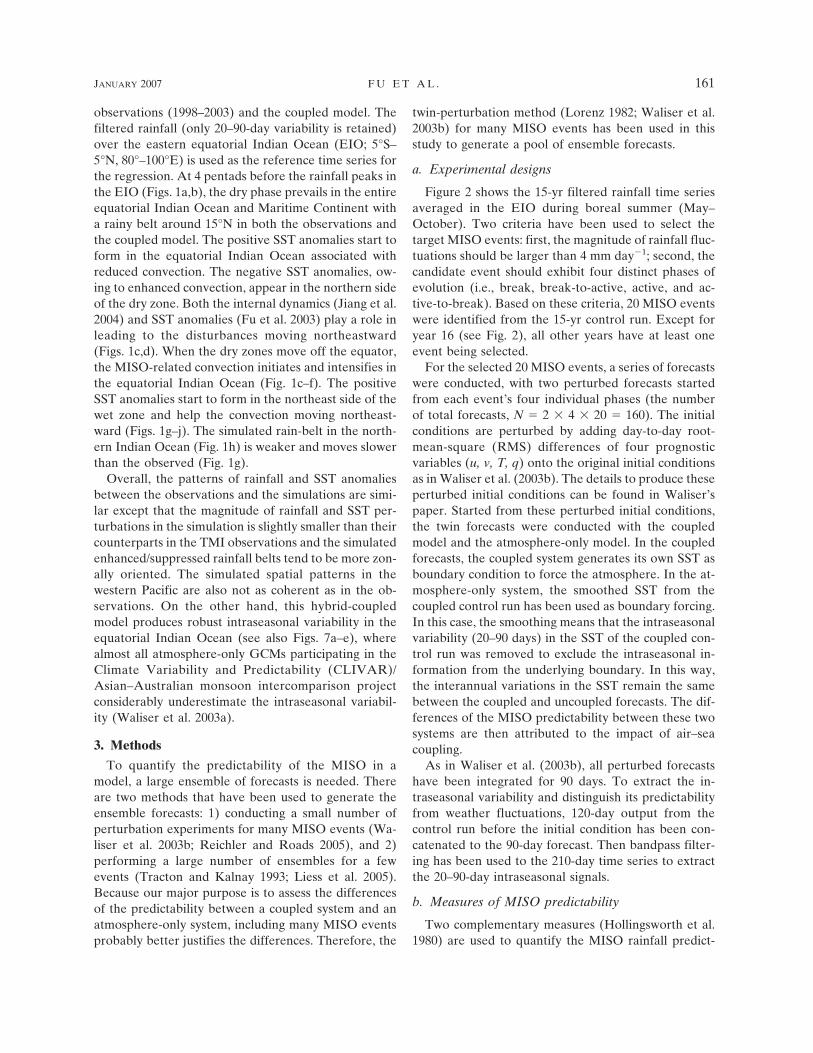
Figure 2 shows the 15-yr filtered rainfall time seriesaveraged in the EIO during boreal summer (May–October). Two criteria have been used to select thetarget MISO events: first, the magnitude of rainfall fluc-tuations should be larger than 4 mm day�1; second, thecandidate event should exhibit four distinct phases ofevolution (i.e., break, break-to-active, active, and ac-tive-to-break). Based on these criteria, 20 MISO eventswere identified from the 15-yr control run. Except foryear 16 (see Fig. 2), all other years have at least oneevent being selected.

For the selected 20 MISO events, a series of forecastswere conducted, with two perturbed forecasts startedfrom each event’s four individual phases (the numberof total forecasts, N � 2 � 4 � 20 � 160). The initialconditions are perturbed by adding day-to-day root-mean-square (RMS) differences of four prognosticvariables (u, v, T, q) onto the original initial conditionsas in Waliser et al. (2003b). The details to produce theseperturbed initial conditions can be found in Waliser’spaper. Started from these perturbed initial conditions,the twin forecasts were conducted with the coupledmodel and the atmosphere-only model. In the coupledforecasts, the coupled system generates its own SST asboundary condition to force the atmosphere. In the at-mosphere-only system, the smoothed SST from thecoupled control run has been used as boundary forcing.In this case, the smoothing means that the intraseasonalvariability (20–90 days) in the SST of the coupled con-trol run was removed to exclude the intraseasonal in-formation from the underlying boundary. In this way,the interannual variations in the SST remain the samebetween the coupled and uncoupled forecasts. The dif-ferences of the MISO predictability between these twosystems are then attributed to the impact of air–seacoupling.

As in Waliser et al. (2003b), all perturbed forecastshave been integrated for 90 days. To extract the in-traseasonal variability and distinguish its predictabilityfrom weather fluctuations, 120-day output from thecontrol run before the initial condition has been con-catenated to the 90-day forecast. Then bandpass filter-ing has been used to the 210-day time series to extractthe 20–90-day intraseasonal signals.

b. Measures of MISO predictability

Two complementary measures (Hollingsworth et al.1980) are used to quantify the MISO rainfall predict-


ability for both the coupled system and the atmosphere-only system. One is the ratio of signal-to-forecast error(Waliser et al. 2003b). The other is the anomaly corre-lation coefficient (Miyakoda et al. 1972; Hollingsworthet al. 1980).

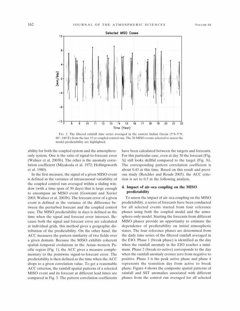
In the first measure, the signal of a given MISO eventis defined as the variance of intraseasonal variability ofthe coupled control run averaged within a sliding win-dow (with a time span of 50 days) that is large enoughto encompass an MISO event (Goswami and Xavier2003; Waliser et al. 2003b). The forecast error of a givenevent is defined as the variance of the difference be-tween the perturbed forecast and the coupled controlcase. The MISO predictability in days is defined as thetime when the signal and forecast error intersect. Be-cause both the signal and forecast error are calculatedat individual grids, this method gives a geographic dis-tribution of the predictability. On the other hand, theACC measures the pattern similarity of two fields overa given domain. Because the MISO exhibits coherentspatial–temporal evolutions in the Asian–western Pa-cific region (Fig. 1), the ACC gives a measure comple-mentary to the pointwise signal-to-forecast error. Thepredictability is then defined as the time when the ACCdrops to a given correlation value. To get a reasonableACC criterion, the rainfall spatial patterns of a selectedMISO event and its forecast at different lead times arecompared in Fig. 3. The pattern correlation coefficients

have been calculated between the targets and forecasts.For this particular case, even at day 30 the forecast (Fig.3j) still looks skillful compared to the target (Fig. 3i).The corresponding pattern correlation coefficient isabout 0.43 at this time. Based on this result and previ-ous study (Reichler and Roads 2005), the ACC crite-rion is set to 0.5 in the following analysis.

4. Impact of air–sea coupling on the MISOpredictability

To assess the impact of air–sea coupling on the MISOpredictability, a series of forecasts have been conductedfor all selected events started from four referencephases using both the coupled model and the atmo-sphere-only model. Starting the forecasts from differentMISO phases provide an opportunity to estimate thedependence of predictability on initial atmosphericstates. The four reference phases are determined fromthe daily time series of the filtered rainfall averaged inthe EIO. Phase 1 (break phase) is identified as the daywhen the rainfall anomaly in the EIO reaches a mini-mum. Phase 2 (break-to-active) corresponds to the daywhen the rainfall anomaly crosses zero from negative topositive. Phase 3 is the peak active phase and phase 4represents the transition day from active to breakphase. Figure 4 shows the composite spatial patterns ofrainfall and SST anomalies associated with differentphases from the control run averaged for all selected

FIG. 2. The filtered rainfall time series averaged in the eastern Indian Ocean (5°S–5°N,80°–100°E) from the last 15-yr coupled control run. The 20 MISO events selected to assess themodel predictability are highlighted.


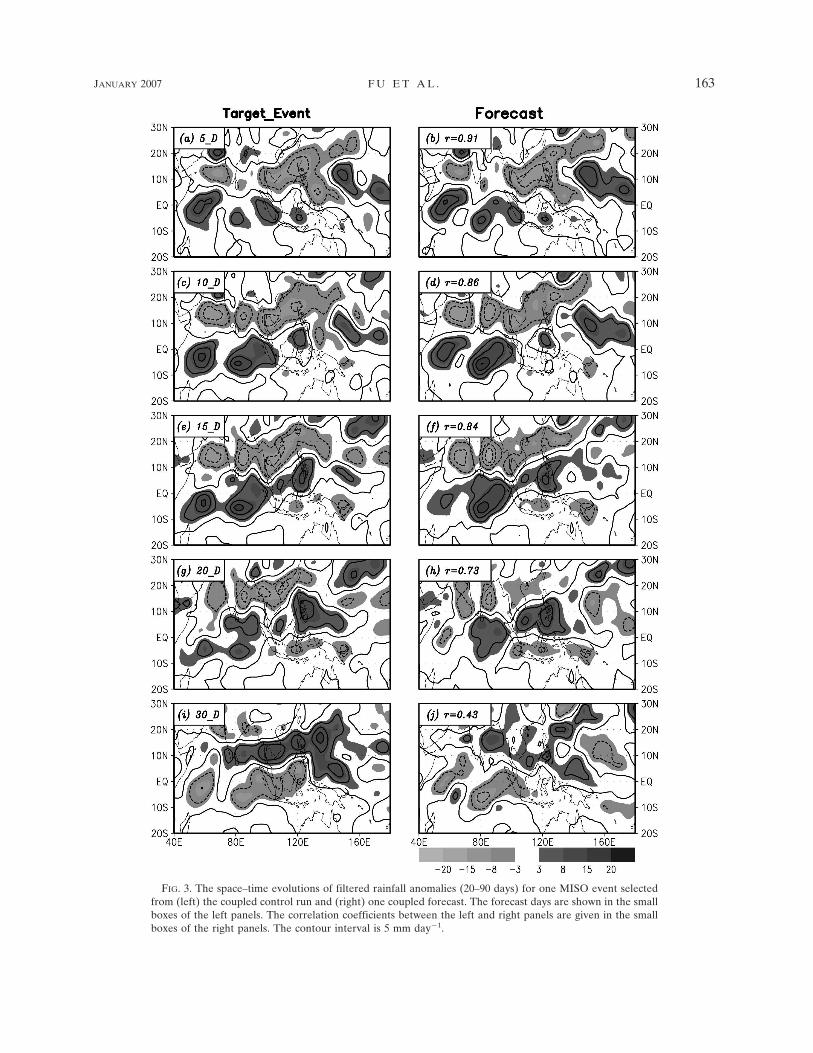
FIG. 3. The space–time evolutions of filtered rainfall anomalies (20–90 days) for one MISO event selectedfrom (left) the coupled control run and (right) one coupled forecast. The forecast days are shown in the smallboxes of the left panels. The correlation coefficients between the left and right panels are given in the smallboxes of the right panels. The contour interval is 5 mm day�1.


events. Generally speaking, the composite phase 1, 2, 3,and 4 correspond to the �4, �2, 0, and �2 pentads inthe regression analysis, respectively (Fig. 1).

a. MISO predictability measured by thesignal-to-error ratio

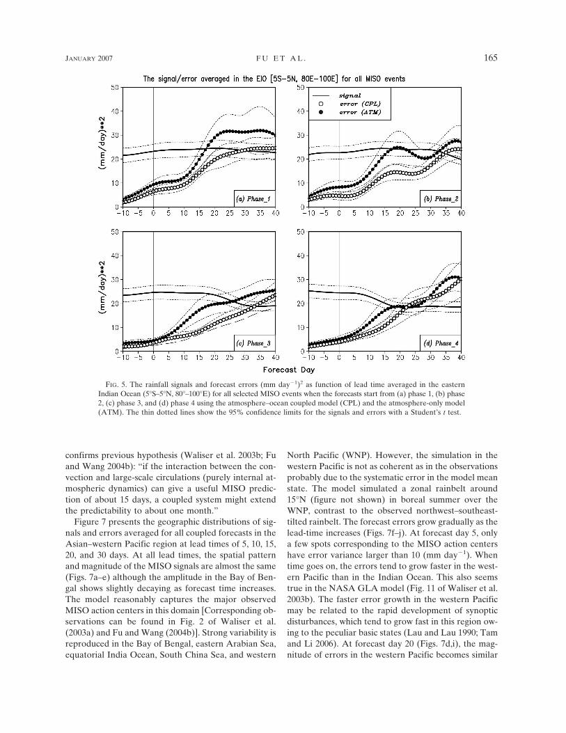
The signals and forecast errors of all the selectedMISO events at their associated four phases have beencalculated at individual grid points. Figure 5 shows thesignals and forecast errors averaged over the EIO asfunction of forecast days at each phase in both thecoupled model and the atmosphere-only model. For allphases, the signals don’t change much as forecast timeincreases, but the forecast errors grow steadily. In thecoupled system, the MISO predictability, defined as thetime when forecast error intersects with the signal, isabout 29, 35, 33, and 22 days, respectively, for phase 1to 4 (Figs. 5a–d).1 In the atmosphere-only model, the

forecast errors grow considerably faster than theircounterparts in the coupled system. The correspondingpredictability in the atmosphere-only model is about17, 17, 26, and 18 days from phase 1 to 4. In general, thepredictability of the coupled model is systematicallyhigher than that of the atmosphere-only model. In thisparticular region, the forecasts started from phase 3(active) have longer predictability than those startedfrom phase 1 (break). This predictability difference be-tween two specific phases is more outstanding in theatmosphere-only model than that in the coupled model.We will come back to this point later.

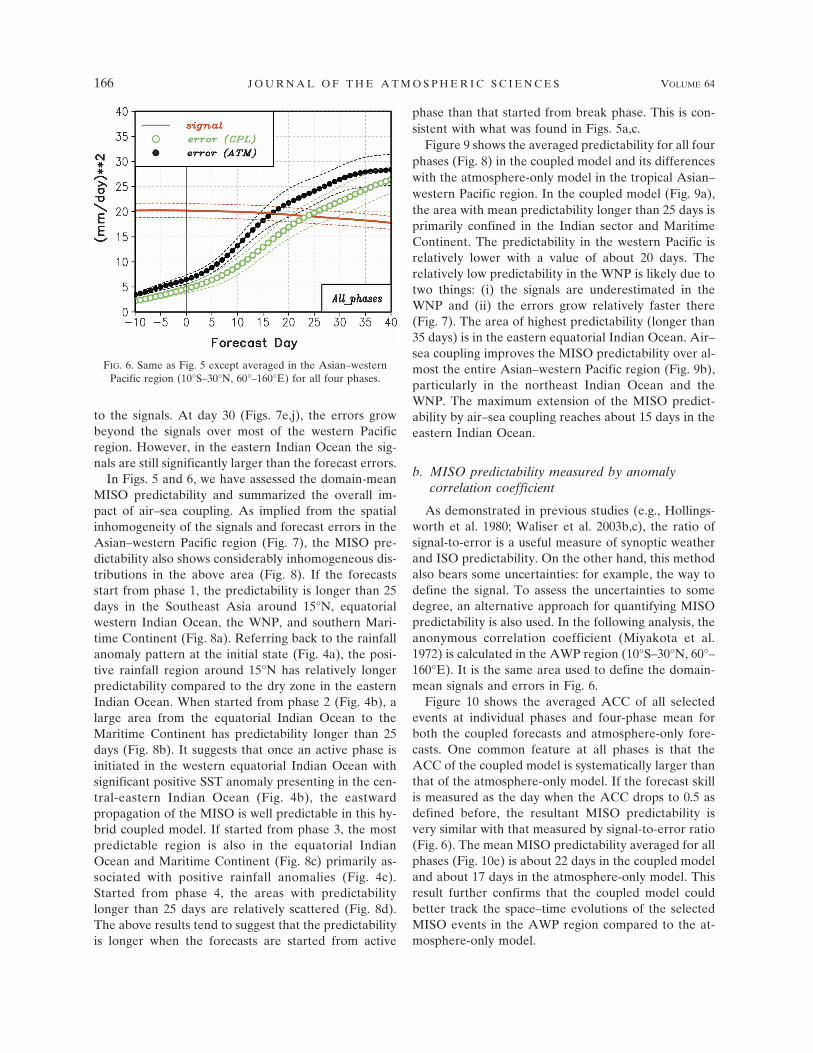
To get an overall view of the MISO predictability inits most active region, the signals and errors of all fore-casts for four phases have been averaged over the tropi-cal Asian–western Pacific domain (AWP; 10°S–30°N,60°–160°E). The averaged MISO predictability of allfour phases in the AWP domain is about 24 days for thecoupled system and 17 days for the atmosphere-onlysystem (Fig. 6). This difference suggests that the air–seacoupling acts to extend the MISO predictability byabout a week in the AWP region. This result somewhat

1 The nonzero errors before the start of forecasts are due to theuse of filtering.

FIG. 4. Composite rainfall (shaded; mm day�1) and SST (contour interval: 0.05°C) anomalies for all selected MISO events at(a) phase 1, (b) phase 2, (c) phase 3, and (d) phase 4.


confirms previous hypothesis (Waliser et al. 2003b; Fuand Wang 2004b): “if the interaction between the con-vection and large-scale circulations (purely internal at-mospheric dynamics) can give a useful MISO predic-tion of about 15 days, a coupled system might extendthe predictability to about one month.”

Figure 7 presents the geographic distributions of sig-nals and errors averaged for all coupled forecasts in theAsian–western Pacific region at lead times of 5, 10, 15,20, and 30 days. At all lead times, the spatial patternand magnitude of the MISO signals are almost the same(Figs. 7a–e) although the amplitude in the Bay of Ben-gal shows slightly decaying as forecast time increases.The model reasonably captures the major observedMISO action centers in this domain [Corresponding ob-servations can be found in Fig. 2 of Waliser et al.(2003a) and Fu and Wang (2004b)]. Strong variability isreproduced in the Bay of Bengal, eastern Arabian Sea,equatorial India Ocean, South China Sea, and western

North Pacific (WNP). However, the simulation in thewestern Pacific is not as coherent as in the observationsprobably due to the systematic error in the model meanstate. The model simulated a zonal rainbelt around15°N (figure not shown) in boreal summer over theWNP, contrast to the observed northwest–southeast-tilted rainbelt. The forecast errors grow gradually as thelead-time increases (Figs. 7f–j). At forecast day 5, onlya few spots corresponding to the MISO action centershave error variance larger than 10 (mm day�1). Whentime goes on, the errors tend to grow faster in the west-ern Pacific than in the Indian Ocean. This also seemstrue in the NASA GLA model (Fig. 11 of Waliser et al.2003b). The faster error growth in the western Pacificmay be related to the rapid development of synopticdisturbances, which tend to grow fast in this region ow-ing to the peculiar basic states (Lau and Lau 1990; Tamand Li 2006). At forecast day 20 (Figs. 7d,i), the mag-nitude of errors in the western Pacific becomes similar

FIG. 5. The rainfall signals and forecast errors (mm day�1)2 as function of lead time averaged in the easternIndian Ocean (5°S–5°N, 80°–100°E) for all selected MISO events when the forecasts start from (a) phase 1, (b) phase2, (c) phase 3, and (d) phase 4 using the atmosphere–ocean coupled model (CPL) and the atmosphere-only model(ATM). The thin dotted lines show the 95% confidence limits for the signals and errors with a Student’s t test.


to the signals. At day 30 (Figs. 7e,j), the errors growbeyond the signals over most of the western Pacificregion. However, in the eastern Indian Ocean the sig-nals are still significantly larger than the forecast errors.

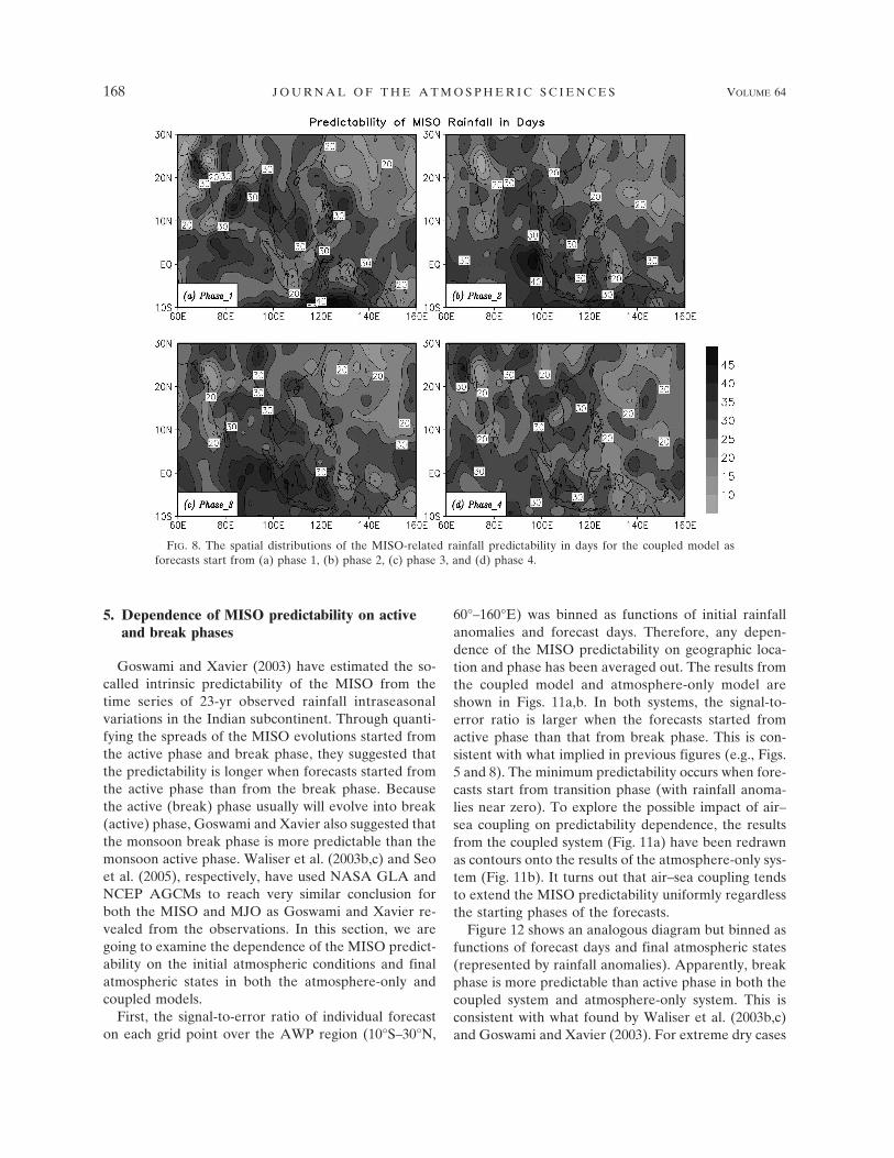
In Figs. 5 and 6, we have assessed the domain-meanMISO predictability and summarized the overall im-pact of air–sea coupling. As implied from the spatialinhomogeneity of the signals and forecast errors in theAsian–western Pacific region (Fig. 7), the MISO pre-dictability also shows considerably inhomogeneous dis-tributions in the above area (Fig. 8). If the forecastsstart from phase 1, the predictability is longer than 25days in the Southeast Asia around 15°N, equatorialwestern Indian Ocean, the WNP, and southern Mari-time Continent (Fig. 8a). Referring back to the rainfallanomaly pattern at the initial state (Fig. 4a), the posi-tive rainfall region around 15°N has relatively longerpredictability compared to the dry zone in the easternIndian Ocean. When started from phase 2 (Fig. 4b), alarge area from the equatorial Indian Ocean to theMaritime Continent has predictability longer than 25days (Fig. 8b). It suggests that once an active phase isinitiated in the western equatorial Indian Ocean withsignificant positive SST anomaly presenting in the cen-tral-eastern Indian Ocean (Fig. 4b), the eastwardpropagation of the MISO is well predictable in this hy-brid coupled model. If started from phase 3, the mostpredictable region is also in the equatorial IndianOcean and Maritime Continent (Fig. 8c) primarily as-sociated with positive rainfall anomalies (Fig. 4c).Started from phase 4, the areas with predictabilitylonger than 25 days are relatively scattered (Fig. 8d).The above results tend to suggest that the predictabilityis longer when the forecasts are started from active

phase than that started from break phase. This is con-sistent with what was found in Figs. 5a,c.

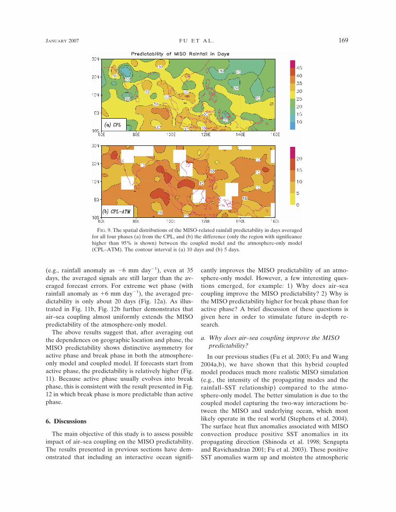
Figure 9 shows the averaged predictability for all fourphases (Fig. 8) in the coupled model and its differenceswith the atmosphere-only model in the tropical Asian–western Pacific region. In the coupled model (Fig. 9a),the area with mean predictability longer than 25 days isprimarily confined in the Indian sector and MaritimeContinent. The predictability in the western Pacific isrelatively lower with a value of about 20 days. Therelatively low predictability in the WNP is likely due totwo things: (i) the signals are underestimated in theWNP and (ii) the errors grow relatively faster there(Fig. 7). The area of highest predictability (longer than35 days) is in the eastern equatorial Indian Ocean. Air–sea coupling improves the MISO predictability over al-most the entire Asian–western Pacific region (Fig. 9b),particularly in the northeast Indian Ocean and theWNP. The maximum extension of the MISO predict-ability by air–sea coupling reaches about 15 days in theeastern Indian Ocean.

b. MISO predictability measured by anomalycorrelation coefficient

As demonstrated in previous studies (e.g., Hollings-worth et al. 1980; Waliser et al. 2003b,c), the ratio ofsignal-to-error is a useful measure of synoptic weatherand ISO predictability. On the other hand, this methodalso bears some uncertainties: for example, the way todefine the signal. To assess the uncertainties to somedegree, an alternative approach for quantifying MISOpredictability is also used. In the following analysis, theanonymous correlation coefficient (Miyakota et al.1972) is calculated in the AWP region (10°S–30°N, 60°–160°E). It is the same area used to define the domain-mean signals and errors in Fig. 6.

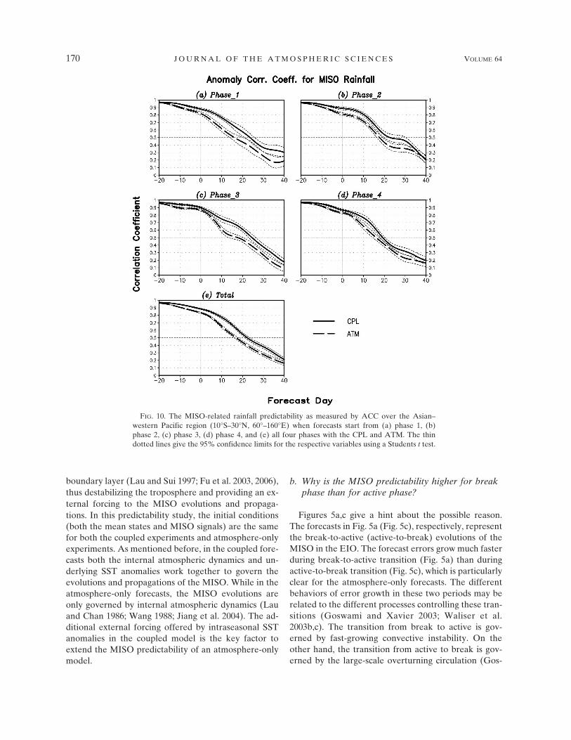
Figure 10 shows the averaged ACC of all selectedevents at individual phases and four-phase mean forboth the coupled forecasts and atmosphere-only fore-casts. One common feature at all phases is that theACC of the coupled model is systematically larger thanthat of the atmosphere-only model. If the forecast skillis measured as the day when the ACC drops to 0.5 asdefined before, the resultant MISO predictability isvery similar with that measured by signal-to-error ratio(Fig. 6). The mean MISO predictability averaged for allphases (Fig. 10e) is about 22 days in the coupled modeland about 17 days in the atmosphere-only model. Thisresult further confirms that the coupled model couldbetter track the space–time evolutions of the selectedMISO events in the AWP region compared to the at-mosphere-only model.

FIG. 6. Same as Fig. 5 except averaged in the Asian–westernPacific region (10°S–30°N, 60°–160°E) for all four phases.


Fig 6 live 4/C

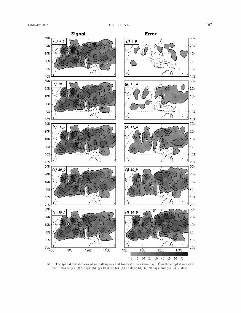
FIG. 7. The spatial distributions of rainfall signals and forecast errors (mm day�1)2 in the coupled model atlead times of (a), (f) 5 days; (b), (g) 10 days; (c), (h) 15 days; (d), (i) 20 days; and (e), (j) 30 days.


5. Dependence of MISO predictability on activeand break phases

Goswami and Xavier (2003) have estimated the so-called intrinsic predictability of the MISO from thetime series of 23-yr observed rainfall intraseasonalvariations in the Indian subcontinent. Through quanti-fying the spreads of the MISO evolutions started fromthe active phase and break phase, they suggested thatthe predictability is longer when forecasts started fromthe active phase than from the break phase. Becausethe active (break) phase usually will evolve into break(active) phase, Goswami and Xavier also suggested thatthe monsoon break phase is more predictable than themonsoon active phase. Waliser et al. (2003b,c) and Seoet al. (2005), respectively, have used NASA GLA andNCEP AGCMs to reach very similar conclusion forboth the MISO and MJO as Goswami and Xavier re-vealed from the observations. In this section, we aregoing to examine the dependence of the MISO predict-ability on the initial atmospheric conditions and finalatmospheric states in both the atmosphere-only andcoupled models.

First, the signal-to-error ratio of individual forecaston each grid point over the AWP region (10°S–30°N,

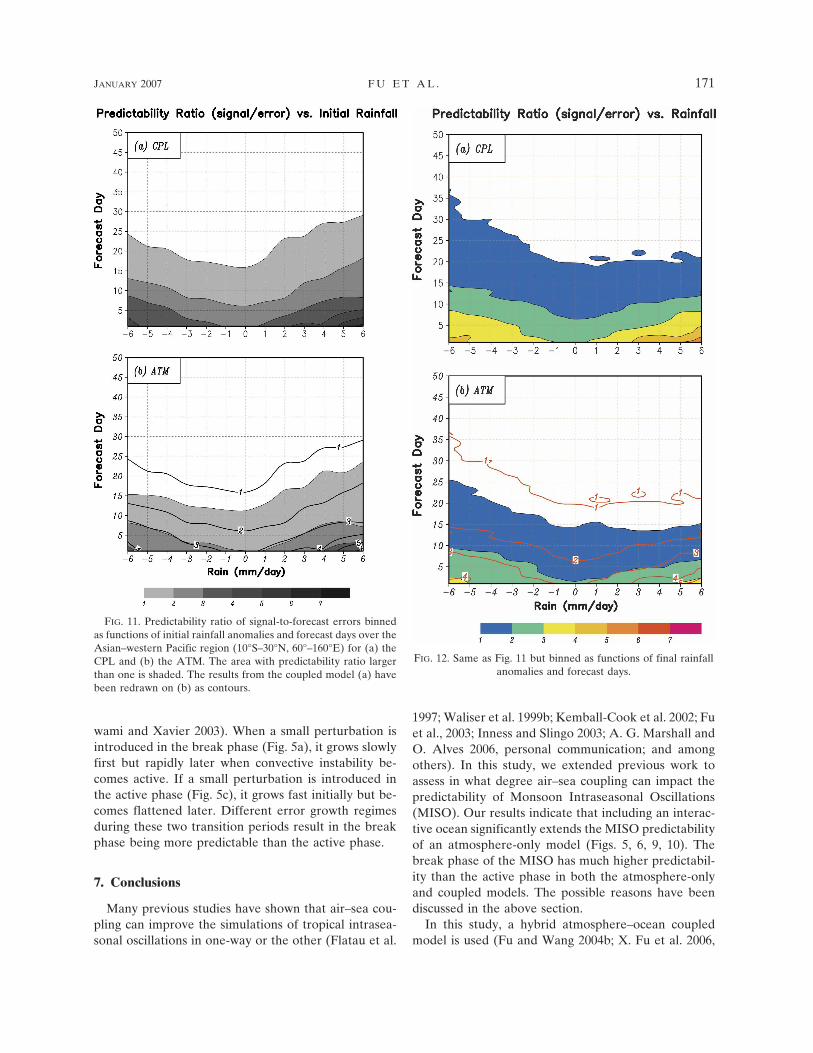
60°–160°E) was binned as functions of initial rainfallanomalies and forecast days. Therefore, any depen-dence of the MISO predictability on geographic loca-tion and phase has been averaged out. The results fromthe coupled model and atmosphere-only model areshown in Figs. 11a,b. In both systems, the signal-to-error ratio is larger when the forecasts started fromactive phase than that from break phase. This is con-sistent with what implied in previous figures (e.g., Figs.5 and 8). The minimum predictability occurs when fore-casts start from transition phase (with rainfall anoma-lies near zero). To explore the possible impact of air–sea coupling on predictability dependence, the resultsfrom the coupled system (Fig. 11a) have been redrawnas contours onto the results of the atmosphere-only sys-tem (Fig. 11b). It turns out that air–sea coupling tendsto extend the MISO predictability uniformly regardlessthe starting phases of the forecasts.

Figure 12 shows an analogous diagram but binned asfunctions of forecast days and final atmospheric states(represented by rainfall anomalies). Apparently, breakphase is more predictable than active phase in both thecoupled system and atmosphere-only system. This isconsistent with what found by Waliser et al. (2003b,c)and Goswami and Xavier (2003). For extreme dry cases

FIG. 8. The spatial distributions of the MISO-related rainfall predictability in days for the coupled model asforecasts start from (a) phase 1, (b) phase 2, (c) phase 3, and (d) phase 4.


(e.g., rainfall anomaly as �6 mm day�1), even at 35days, the averaged signals are still larger than the av-eraged forecast errors. For extreme wet phase (withrainfall anomaly as �6 mm day�1), the averaged pre-dictability is only about 20 days (Fig. 12a). As illus-trated in Fig. 11b, Fig. 12b further demonstrates thatair–sea coupling almost uniformly extends the MISOpredictability of the atmosphere-only model.

The above results suggest that, after averaging outthe dependences on geographic location and phase, theMISO predictability shows distinctive asymmetry foractive phase and break phase in both the atmosphere-only model and coupled model. If forecasts start fromactive phase, the predictability is relatively higher (Fig.11). Because active phase usually evolves into breakphase, this is consistent with the result presented in Fig.12 in which break phase is more predictable than activephase.

6. Discussions

The main objective of this study is to assess possibleimpact of air–sea coupling on the MISO predictability.The results presented in previous sections have dem-onstrated that including an interactive ocean signifi-

cantly improves the MISO predictability of an atmo-sphere-only model. However, a few interesting ques-tions emerged, for example: 1) Why does air–seacoupling improve the MISO predictability? 2) Why isthe MISO predictability higher for break phase than foractive phase? A brief discussion of these questions isgiven here in order to stimulate future in-depth re-search.

a. Why does air–sea coupling improve the MISOpredictability?

In our previous studies (Fu et al. 2003; Fu and Wang2004a,b), we have shown that this hybrid coupledmodel produces much more realistic MISO simulation(e.g., the intensity of the propagating modes and therainfall–SST relationship) compared to the atmo-sphere-only model. The better simulation is due to thecoupled model capturing the two-way interactions be-tween the MISO and underlying ocean, which mostlikely operate in the real world (Stephens et al. 2004).The surface heat flux anomalies associated with MISOconvection produce positive SST anomalies in itspropagating direction (Shinoda et al. 1998; Senguptaand Ravichandran 2001; Fu et al. 2003). These positiveSST anomalies warm up and moisten the atmospheric

FIG. 9. The spatial distributions of the MISO-related rainfall predictability in days averagedfor all four phases (a) from the CPL, and (b) the difference (only the region with significancehigher than 95% is shown) between the coupled model and the atmosphere-only model(CPL–ATM). The contour interval is (a) 10 days and (b) 5 days.


Fig 9 live 4/C

boundary layer (Lau and Sui 1997; Fu et al. 2003, 2006),thus destabilizing the troposphere and providing an ex-ternal forcing to the MISO evolutions and propaga-tions. In this predictability study, the initial conditions(both the mean states and MISO signals) are the samefor both the coupled experiments and atmosphere-onlyexperiments. As mentioned before, in the coupled fore-casts both the internal atmospheric dynamics and un-derlying SST anomalies work together to govern theevolutions and propagations of the MISO. While in theatmosphere-only forecasts, the MISO evolutions areonly governed by internal atmospheric dynamics (Lauand Chan 1986; Wang 1988; Jiang et al. 2004). The ad-ditional external forcing offered by intraseasonal SSTanomalies in the coupled model is the key factor toextend the MISO predictability of an atmosphere-onlymodel.

b. Why is the MISO predictability higher for breakphase than for active phase?

Figures 5a,c give a hint about the possible reason.The forecasts in Fig. 5a (Fig. 5c), respectively, representthe break-to-active (active-to-break) evolutions of theMISO in the EIO. The forecast errors grow much fasterduring break-to-active transition (Fig. 5a) than duringactive-to-break transition (Fig. 5c), which is particularlyclear for the atmosphere-only forecasts. The differentbehaviors of error growth in these two periods may berelated to the different processes controlling these tran-sitions (Goswami and Xavier 2003; Waliser et al.2003b,c). The transition from break to active is gov-erned by fast-growing convective instability. On theother hand, the transition from active to break is gov-erned by the large-scale overturning circulation (Gos-

FIG. 10. The MISO-related rainfall predictability as measured by ACC over the Asian–western Pacific region (10°S–30°N, 60°–160°E) when forecasts start from (a) phase 1, (b)phase 2, (c) phase 3, (d) phase 4, and (e) all four phases with the CPL and ATM. The thindotted lines give the 95% confidence limits for the respective variables using a Students t test.


wami and Xavier 2003). When a small perturbation isintroduced in the break phase (Fig. 5a), it grows slowlyfirst but rapidly later when convective instability be-comes active. If a small perturbation is introduced inthe active phase (Fig. 5c), it grows fast initially but be-comes flattened later. Different error growth regimesduring these two transition periods result in the breakphase being more predictable than the active phase.

7. Conclusions

Many previous studies have shown that air–sea cou-pling can improve the simulations of tropical intrasea-sonal oscillations in one-way or the other (Flatau et al.

1997; Waliser et al. 1999b; Kemball-Cook et al. 2002; Fuet al., 2003; Inness and Slingo 2003; A. G. Marshall andO. Alves 2006, personal communication; and amongothers). In this study, we extended previous work toassess in what degree air–sea coupling can impact thepredictability of Monsoon Intraseasonal Oscillations(MISO). Our results indicate that including an interac-tive ocean significantly extends the MISO predictabilityof an atmosphere-only model (Figs. 5, 6, 9, 10). Thebreak phase of the MISO has much higher predictabil-ity than the active phase in both the atmosphere-onlyand coupled models. The possible reasons have beendiscussed in the above section.

In this study, a hybrid atmosphere–ocean coupledmodel is used (Fu and Wang 2004b; X. Fu et al. 2006,

FIG. 11. Predictability ratio of signal-to-forecast errors binnedas functions of initial rainfall anomalies and forecast days over theAsian–western Pacific region (10°S–30°N, 60°–160°E) for (a) theCPL and (b) the ATM. The area with predictability ratio largerthan one is shaded. The results from the coupled model (a) havebeen redrawn on (b) as contours.

FIG. 12. Same as Fig. 11 but binned as functions of final rainfallanomalies and forecast days.


Fig 12 live 4/C

unpublished manuscript). It reasonably simulates themajor observed characteristics of the MISO over theAsian–western Pacific region, particularly in the Indiansector (Fig. 1, see also the validations in Fu et al. 2003;Fu and Wang 2004b; X. Fu et al. 2006, unpublishedmanuscript). To assess the model predictability of theMISO, 20 intraseasonal events during boreal summerhave been selected from a 15-yr control run (Fig. 2).Four phases (i.e., break, break-to-active, active, and ac-tive-to-break) are defined for individual MISO eventsbased on the rainfall time series at the eastern IndianOcean (5°S–5°N, 80°–100°E). A series of twin pertur-bation forecasts have been conducted for each phase ofall selected MISO events using both the coupled modeland the atmosphere-only model. Two complementarymeasures are used to quantify the MISO predictability:(i) the ratio of signal-to-forecast error, and (ii) the spa-tial anomaly correlation coefficient (ACC).

When measured with the ratio of signal-to-forecasterror, the predictability in the tropical Indian sector isgenerally higher than that in the western North Pacific(Fig. 9a). The relatively lower predictability in theWNP is probably due to two reasons. First, the MISOvariability (i.e., the signal) in this region is underesti-mated (Figs. 7a–e). Second, the forecast errors tend togrow faster in the WNP (Figs. 7f–j) probably owing tothe intrinsic instability (Lau and Lau 1990). Air–seacoupling extends the MISO predictability almost overthe entire Asian–western Pacific domain (Fig. 9b). Av-eraged over this area (10°S–30°N, 60°–160°E), the pre-dictability of the MISO-related rainfall reaches about24 days in the coupled model and is about 17 days in theatmosphere-only model (Fig. 6). Very similar conclu-sion was obtained when measured with the anomalycorrelation coefficient (Fig. 10). These results suggestthat air–sea coupling is able to extend the predictabilityof the MISO-related rainfall by about a week in its mostactive domain.

The predictability of the MISO is phase dependent inboth the atmosphere-only model and the coupledmodel (Figs. 11, 12). The predictability is higher whenforecasts start from active phase than that from breakphase (Fig. 11), the result of which is that the breakphase of the MISO is more predictable than the activephase (Fig. 12). This is consistent with what found fromprevious observational and modeling studies (Goswamiand Xavier 2003; Waliser et al. 2003a,b). Air–sea cou-pling almost uniformly extends the predictability of theMISO for all phases (Figs. 11b, 12b).

Because both the coupled forecasts and atmosphere-only forecasts have same initial conditions, the exten-sion of MISO predictability in the coupled case canonly come from the intraseasonal SST anomalies, which

have been removed from the atmosphere-only fore-casts. The almost uniform enhancement of MISO pre-dictability by air–sea coupling (Figs. 11b, 12b) suggeststhat both the positive and negative intraseasonal SSTanomalies play equally important role. The positiveSST anomalies destabilize the atmosphere ahead of theconvection. At the same time, the negative SST anoma-lies stabilize the atmosphere below the convection.Both processes help the MISO-related convectionpropagate northeastward.

In this study, we only assessed the impact of air–seacoupling on the MISO predictability in boreal summer.Further experiments could be conducted to estimatethe impact of air–sea coupling on the MJO predictabil-ity in boreal winter. Most experiments we have done incurrent study consider only two scenarios: fully atmo-sphere–ocean coupled model and atmosphere-onlymodel forced with smoothed SST. To thoroughly un-derstand the impacts of underlying boundary condi-tions on the MISO predictability, a few more sensitivityexperiments should be conducted: for example, usingdaily SST or damped persistent SST to force the atmo-spheric model and introducing a simple oceanic mixedlayer into the atmospheric model. Our future researchwill address these issues.

Acknowledgments. This work was supported byNASA Earth Science Program (NNG04GL65G), byNSF Climate Dynamics Program (ATM03-29531), andby the Japan Agency for Marine–Earth Science andTechnology (JAMSTEC) through its sponsorship of theIPRC. The third author was supported by the HumanResources Development Fund at the Jet PropulsionLaboratory (JPL), as well as the NSF (ATM-0094416),and the National Atmospheric and Aeronautics Ad-ministration (NAG5- 11033). The research at JPL, Cali-fornia Institute of Technology was performed undercontracts with the NASA. Comments from two anony-mous reviewers greatly help improve the manuscript.

REFERENCES

Arakawa, O., and A. Kitoh, 2004: Comparison of local precipita-tion-SST relationship between the observation and a reanaly-sis dataset. Geophys. Res. Lett., 31, L12206, doi:10.1029/2004GL020283.

Chen, T.-C., and J. C. Alpert, 1990: Systematic errors in the an-nual and intraseasonal variations of the planetary-scale di-vergent circulation in NMC medium-range forecasts. Mon.Wea. Rev., 118, 2607–2623.

Dumenil, L., and E. Todini, 1992: A rainfall-runoff scheme for usein the Hamburg climate model. Advances in Theoretical Hy-drology, A Tribute to James Dooge, European GeophysicalSociety Series on Hydrological Sciences, Vol. 1, ElsevierPress, 129–157.


Flatau, M., P. Flatau, P. Phoebus, and P. Niller, 1997: The feed-back between equatorial convection and local radiative andevaporative processes: The implications for intraseasonal os-cillations. J. Atmos. Sci., 54, 2373–2386.

Fu, X., and B. Wang, 2001: A coupled modeling study of theseasonal cycle of the Pacific cold tongue. Part I: Simulationand sensitivity experiments. J. Climate, 14, 765–779.

——, and ——, 2004a: Differences of boreal-summer intrasea-sonal oscillations simulated in an atmosphere–ocean coupledmodel and an atmosphere-only model. J. Climate, 17, 1263–1271.

——, and ——, 2004b: The boreal-summer intraseasonal oscilla-tions simulated in a hybrid coupled atmosphere–oceanmodel. Mon. Wea. Rev., 132, 2628–2649.

——, ——, T. Li, and J. P. McCreary, 2003: Coupling betweennorthward-propagating, intraseasonal oscillations and seasurface temperature in the Indian Ocean. J. Atmos. Sci., 60,1733–1753.

——, ——, and L. Tao, 2006: Satellite data reveal the 3-D mois-ture structure of Tropical Intraseasonal Oscillation and itscoupling with underlying ocean. Geophys. Res. Lett., 33,L03705, doi:10.1029/2005GL025074.

Gadgil, S., and P. R. S. Rao, 2000: Famine strategies for a variableclimate—A challenge. Curr. Sci., 78, 1203–1215.

Gaspar, P., 1988: Modeling the seasonal cycle of the upper ocean.J. Phys. Oceanogr., 18, 161–180.

Goswami, B. N., and R. S. Ajayamohan, 2001: Intraseasonal os-cillations and interannual variability of the Indian summermonsoon. J. Climate, 14, 1180–1198.

——, and P. K. Xavier, 2003: Potential predictability and ex-tended range prediction of Indian summer monsoon breaks.Geophys. Res. Lett., 30, 1966, doi:10.1029/2003GL017810.

——, R. S. Ajayamohan, P. K. Xavier, and D. Sengupta, 2003:Clustering of low pressure systems during the Indian summermonsoon by intraseasonal oscillations. Geophys. Res. Lett.,30, 1431, doi:10.1029/2002GL016734.

Hendon, H. H., 2000: Impact of air–sea coupling on the Madden–Julian oscillation in a general circulation model. J. Atmos.Sci., 57, 3939–3952.

——, B. Liebmann, M. Newman, J. D. Glick, and J. E. Schemm,2000: Medium-range forecast errors associated with activeepisodes of the Madden–Julian oscillation. Mon. Wea. Rev.,128, 69–86.

Hollingsworth, A., K. Arpe, M. Tiedtke, M. Capaldo, and H. Savi-jarvi, 1980: The performance of a medium-range forecastmodel in winter—Impact of physical parameterizations. Mon.Wea. Rev., 108, 1736–1773.

IFRC, 2000: World Disaster Report: Focus on Recovery. IFRC,392 pp.

Inness, P. M., and J. M. Slingo, 2003: Simulation of the Madden–Julian oscillation in a coupled general circulation model. PartI: Comparison with observations and an atmosphere-onlyGCM. J. Climate, 16, 345–364.

Jiang, X., T. Li, and B. Wang, 2004: Structures and mechanisms ofthe northward propagating boreal summer intraseasonal os-cillations. J. Climate, 17, 1022–1039.

Jones, C., D. E. Waliser, J.-K. E. Schemm, and W. K. M. Lau,2000: Prediction skill of the Madden and Julian Oscillation indynamical extended range forecasts. Climate Dyn., 16, 273–289.

——, ——, K. M. Lau, and W. Stern, 2004: Global occurrences ofextreme precipitation events and the Madden–Julian oscilla-

tion: Observations and predictability. J. Climate, 17, 4575–4589.

Kalnay, E., 2003: Atmospheric Modeling, Data Assimilation andPredictability. Cambridge University Press, 341 pp.

Kemball-Cook, S., B. Wang, and X. Fu, 2002: Simulation of theISO in the ECHAM4 model: The impact of coupling with anocean model. J. Atmos. Sci., 59, 1433–1453.

Krishnamurti, T. N., M. Subramaniam, D. K. Oosterhof, and G.Daughenbaugh, 1990: Predictability of low-frequency modes.Meteor. Atmos. Phys., 44, 63–83.

——, ——, G. Daughenbaugh, D. Oosterhof, and J. H. Xue, 1992:One-month forecasts of wet and dry spells of the monsoon.Mon. Wea. Rev., 120, 1191–1223.

Lau, K. H., and N. C. Lau, 1990: Observed structure and propa-gation characteristics of tropical summertime synoptic scaledisturbances. Mon. Wea. Rev., 118, 1888–1913.

Lau, K. M., and P. H. Chan, 1986: Aspects of the 40–50-day os-cillation during the northern summer as inferred from out-going longwave radiation. Mon. Wea. Rev., 114, 1354–1367.

——, and F. C. Chang, 1992: Tropical intraseasonal oscillation andits prediction by the NMC operational model. J. Climate, 5,1365–1378.

——, and C.-H. Sui, 1997: Mechanisms of short-term sea surfacetemperature regulation: Observations during TOGACOARE. J. Climate, 10, 465–472.

Liess, S., D. E. Waliser, and S. D. Schubert, 2005: Predictabilitystudies of the intraseasonal oscillation in ECHAM5 GCM. J.Atmos. Sci., 62, 3320–3336.

Lo, F., and H. H. Hendon, 2000: Empirical extended-range pre-diction of the Madden–Julian oscillation. Mon. Wea. Rev.,128, 2528–2543.

Lorenz, E. N., 1982: Atmospheric predictability experiments witha large numerical model. Tellus, 34, 505–513.

Matthews, A. J., 2004: Atmospheric response to observed in-traseasonal tropical sea surface temperature anomalies. Geo-phys. Res. Lett., 31, L14107, doi:10.1029/2004GL020474.

Miyakoda, K., G. D. Hembree, R. F. Strickler, and I. Shulman,1972: Cumulative results of extended forecast experiment. I.Model performance for winter cases. Mon. Wea. Rev., 100,836–855.

McCreary, J. P., and Z. J. Yu, 1992: Equatorial dynamics in a2.5-layer model. Progress in Oceanography, Vol. 29, Perga-mon, 61–132.

Mo, K. C., 2001: Adaptive filtering and prediction of intraseasonaloscillations. Mon. Wea. Rev., 129, 802–817.

Nordeng, T. E., 1994: Extended versions of the convective param-eterization scheme at ECMWF and their impact on the meanand transient activity of the model in the tropics. ECMWFResearch Dept. Tech. Memo. 206, European Centre for Me-dium-Range Weather Forecasts, Reading, United Kingdom,41 pp.

Reichler, T., and J. O. Roads, 2005: Long-range predictability inthe tropics. Part II: 30–60-day variability. J. Climate, 18, 634–650.

Roeckner, E., and Coauthors, 1996: The atmospheric general cir-culation model ECHAM-4: Model description and simula-tion of present-day climate. Tech. Rep., Max-Plank-Institutefor Meteorology, Rep. 218, 90 pp.

Sengupta, D., and M. Ravichandran, 2001: Oscillations of Bay ofBengal sea surface temperature during the 1998 summermonsoon. Geophys. Res. Lett., 28, 2033–2036.

Seo, K.-H., J.-K. Schemm, and C. Jones, 2005: Forecast skill of the


Tropical Intraseasonal Oscillation in the NCEP GFS dynami-cal extended range forecasts. Climate Dyn., 25, 265–284.

Shinoda, T., H. H. Hendon, and J. Glick, 1998: Intraseasonal vari-ability of surface fluxes and sea surface temperature in thetropical western Pacific and Indian Oceans. J. Climate, 11,1685–1702.

Stephens, G. L., P. J. Webster, R. H. Johnson, R. Engelen, and T.L’Ecuyer, 2004: Observational evidence for the mutual regu-lation of the tropical hydrological cycle and tropical sea sur-face temperatures. J. Climate, 17, 2213–2224.

Tam, C. Y., and T. Li, 2006: The origin and dispersion character-istics of the observed summertime synoptic-scale waves overthe western Pacific. Mon. Wea. Rev., 134, 1630–1646.

Taylor, K. E., D. Williamson, and F. Zwiers, 2000: The sea surfacetemperature and sea-ice concentration boundary conditionfor AMIP II simulations. PCMDI Rep. 60, Program for Cli-mate Model Diagnosis and Intercomparison, Lawrence Liv-ermore National Laboratory, 25 pp.

Tiedtke, M., 1989: A comprehensive mass flux scheme for cumu-lus parameterization in large-scale models. Mon. Wea. Rev.,117, 1779–1800.

Tracton, M. S., and E. Kalnay, 1993: Ensemble forecasting atNMC: Practical aspects. Wea. Forecasting, 8, 379–398.

Van den Dool, H. M., and S. Saha, 1990: Frequency dependencein forecast skill. Mon. Wea. Rev., 118, 128–137.

Waliser, D. E., K. M. Lau, and J. H. Kim, 1999a: A statistical ex-tended-range tropical forecast model based on the slow evo-lution of the Madden–Julian oscillation. J. Climate, 12, 1918–1939.

——, ——, and ——, 1999b: The influence of coupled sea surfacetemperatures on the Madden–Julian oscillation: A modelperturbation experiment. J. Atmos. Sci., 56, 333–358.

——, and Coauthors, 2003a: AGCM simulations of intraseasonal

variability associated with the Asian summer monsoon. Cli-mate Dyn., 21, 423–446.

——, W. Stern, S. Schubert, and K. M. Lau, 2003b: Dynamic pre-dictability of intraseasonal variability associated with theAsian summer monsoon. Quart. J. Roy. Meteor. Soc., 129,2897–2925.

——, K. M. Lau, W. Stern, and C. Jones, 2003c: Potential predict-ability of the Madden–Julian oscillation. Bull. Amer. Meteor.Soc., 84, 33–50.

Wang, B., 1988: Dynamics of tropical low-frequency waves: Ananalysis of the moist Kelvin waves. J. Atmos. Sci., 45, 2051–2065.

——, and H. Rui, 1990: Synoptic climatology of transient tropicalintraseasonal convection anomalies: 1975–1985. Meteor. At-mos. Phys., 44, 43–61.

——, and X. Xie, 1998: Coupled modes of the warm pool climatesystem. Part I: The role of air–sea interaction in maintainingMadden–Julian oscillation. J. Climate, 11, 2116–2135.

——, T. Li, and P. Chang, 1995: An intermediate model of thetropical Pacific Ocean. J. Phys. Oceanogr., 25, 1599–1616.

Webster, P. J., and C. Hoyos, 2004: Forecasting monsoon rainfalland river discharge variability on 15–30-day time scales. Bull.Amer. Meteor. Soc., 85, 1745–1765.

——, V. O. Magana, T. N. Palmer, J. Shukla, R. A. Tomas, M.Yanai, and T. Yasunari, 1998: Monsoons: Processes, predict-ability, and the prospects for prediction. J. Geophys. Res., 103(C7) (TOGA special issue), 14 451–14 510.

Yasunari, T., 1980: A quasi-stationary appearance of 30 to 40 dayperiod in the cloudiness fluctuations during the summer mon-soon over India. J. Meteor. Soc. Japan, 58, 225–229.

Zheng, Y., D. E. Waliser, W. F. Stern, and C. Jones, 2004: Therole of coupled sea surface temperatures in the simulation ofthe tropical intraseasonal oscillation. J. Climate, 17, 4109–4134.


Documents

Impact of Atmosphere–Ocean Coupling on the Predictability