Impact of 𝑞!-dependent Drell-Yan data on pion PDFs

Patrick BarryGroup Meeting 3/27/2020

Outline

1. Motivation2. Theory

a. DY & LN theoryb. 𝑞!-dependent DY theory

3. Fitting Methodology4. Results5. Impact of 𝑞! data6. Scale Dependence7. Future works

1. Motivation

Motivation•QCD allows us to study the structure of protonsin terms of partons (quarks, antiquarks, and gluons)•Use factorization theorems to separate hard partonic physics out of soft, non-perturbative objects to quantify structure

4

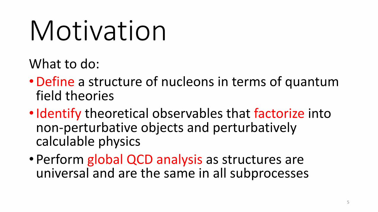
MotivationWhat to do:•Define a structure of nucleons in terms of quantum

field theories• Identify theoretical observables that factorize into

non-perturbative objects and perturbatively calculable physics•Perform global QCD analysis as structures are

universal and are the same in all subprocesses

5

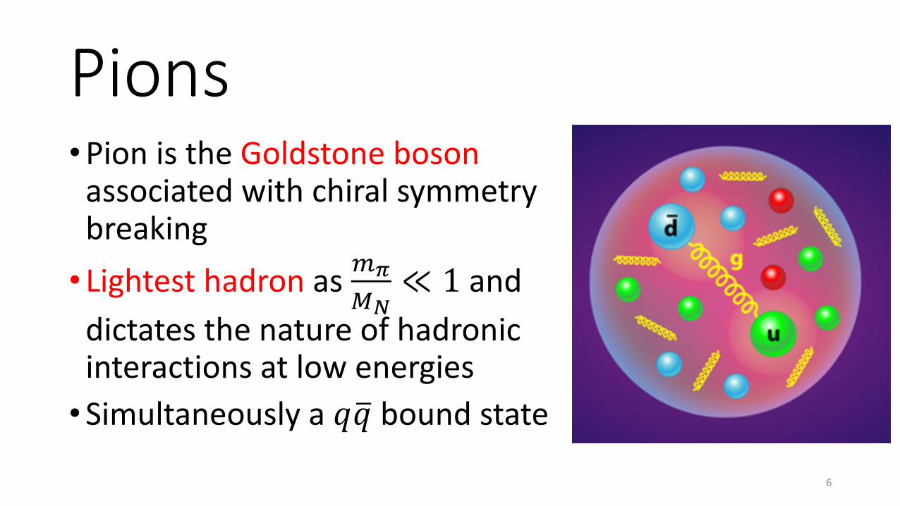
Pions•Pion is the Goldstone boson

associated with chiral symmetry breaking• Lightest hadron as !!

""≪ 1 and

dictates the nature of hadronic interactions at low energies•Simultaneously a 𝑞$𝑞 bound state

6

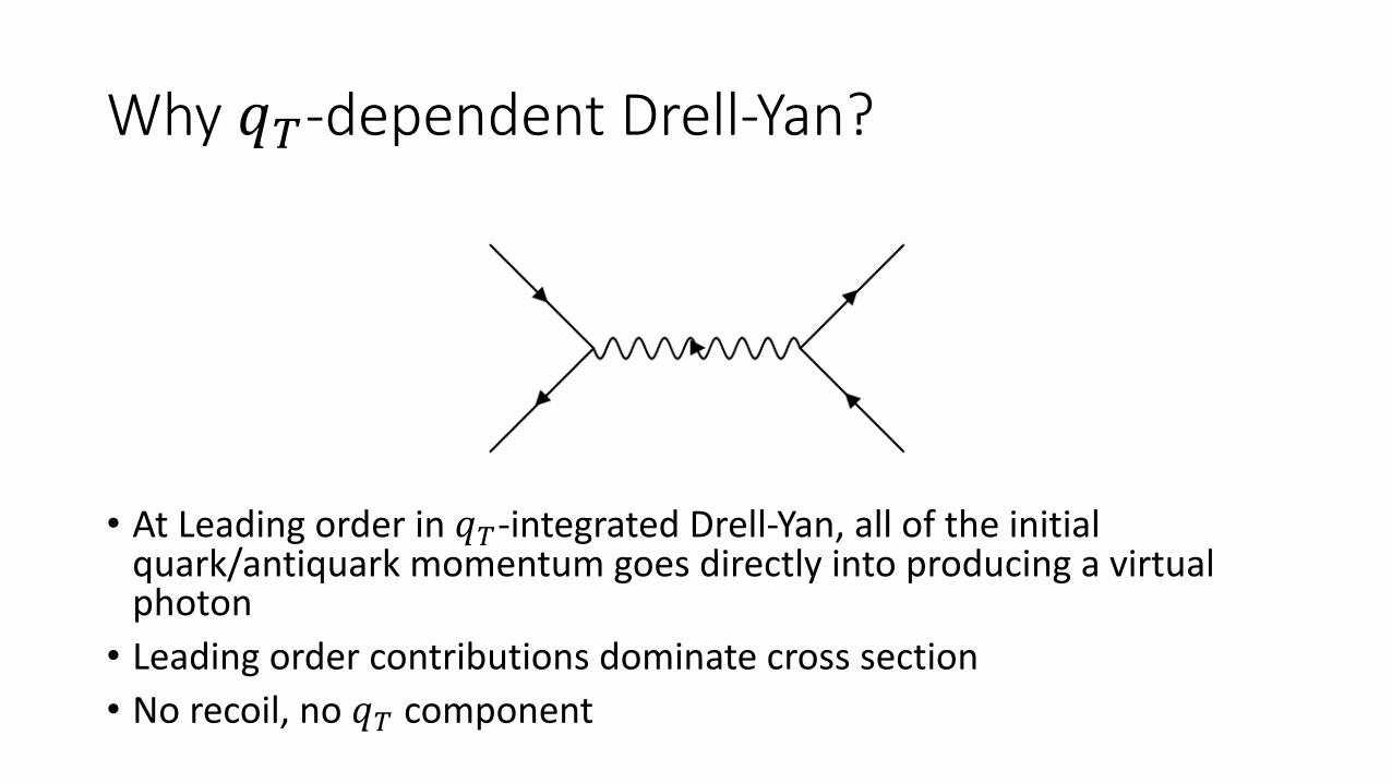
Why 𝑞!-dependent Drell-Yan?

• At Leading order in 𝑞!-integrated Drell-Yan, all of the initial quark/antiquark momentum goes directly into producing a virtual photon• Leading order contributions dominate cross section• No recoil, no 𝑞! component

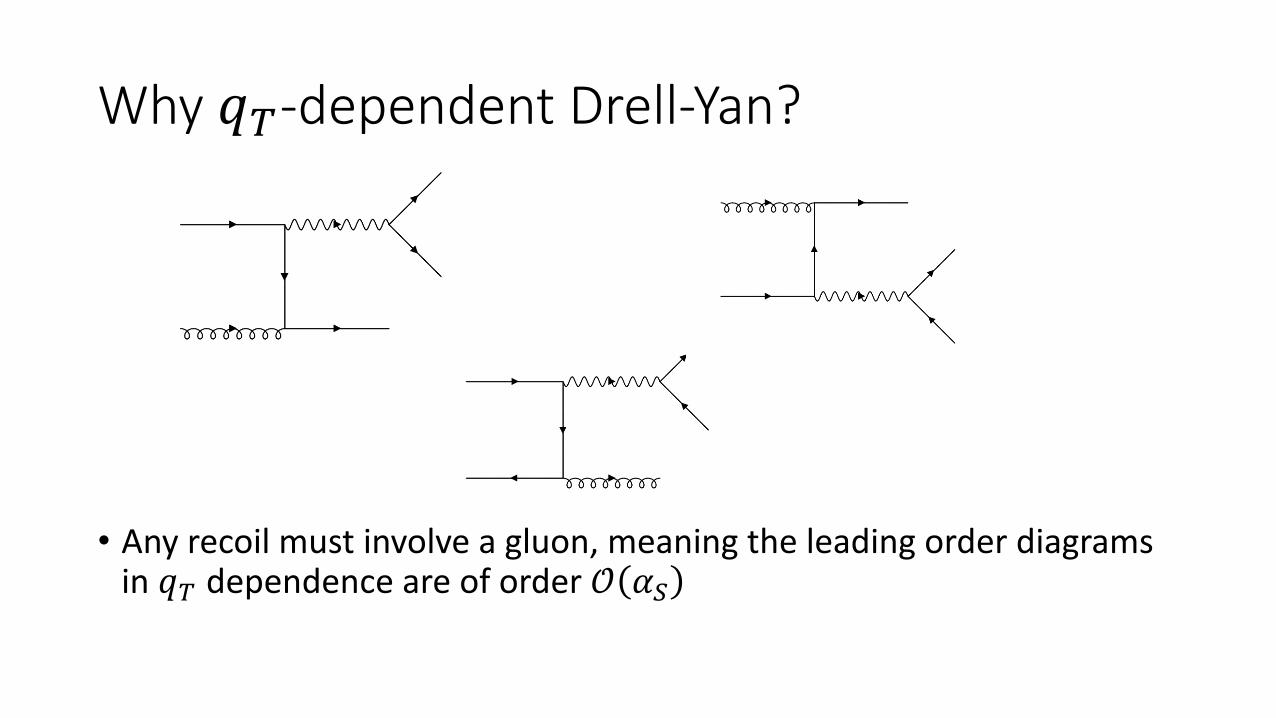
Why 𝑞!-dependent Drell-Yan?

• Any recoil must involve a gluon, meaning the leading order diagrams in 𝑞! dependence are of order 𝒪 𝛼"

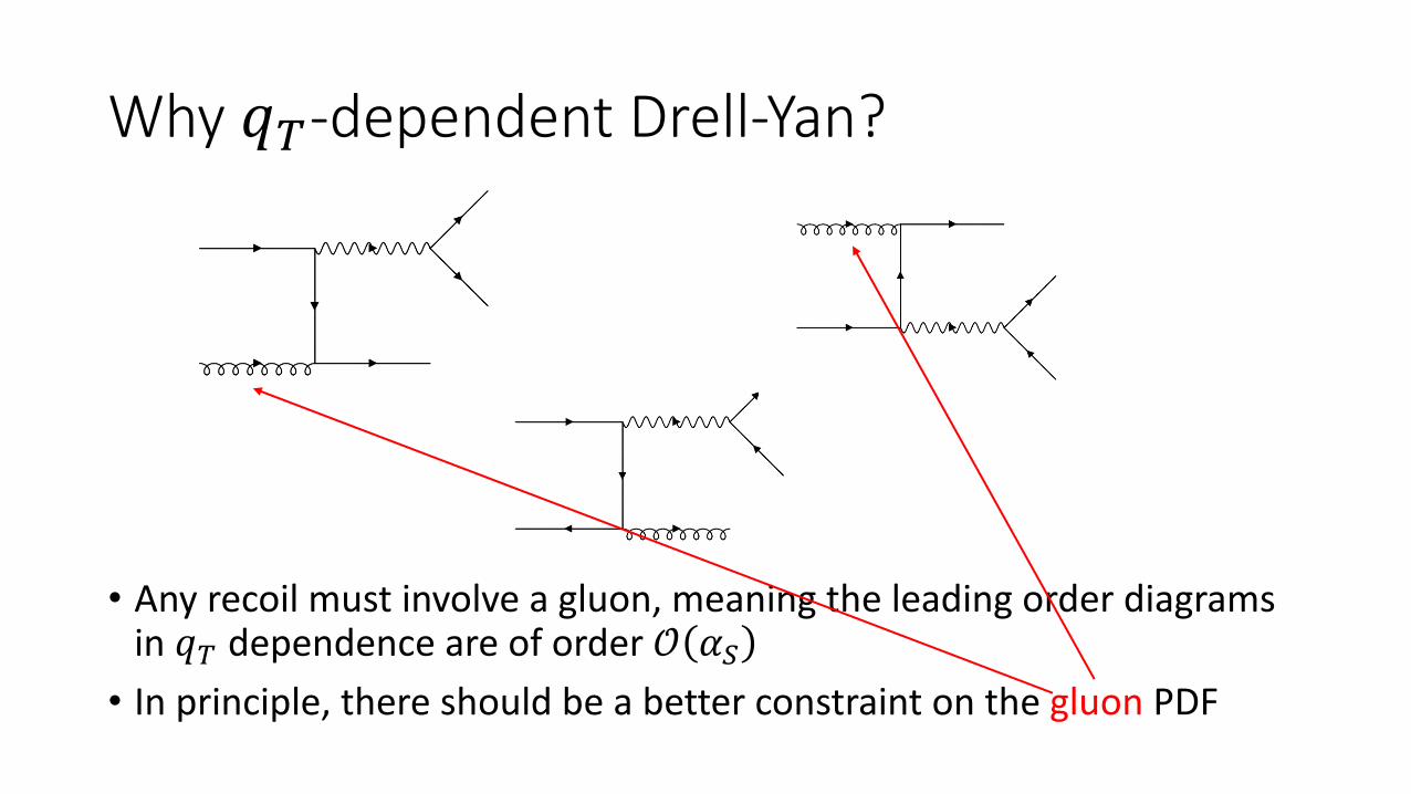
Why 𝑞!-dependent Drell-Yan?

• Any recoil must involve a gluon, meaning the leading order diagrams in 𝑞! dependence are of order 𝒪 𝛼"• In principle, there should be a better constraint on the gluon PDF

Motivation

• There also has not been a successful analysis of collinear PDFs fit to 𝑞!-dependent data• Studying the fixed-order perturbative calculation in 𝑞! has

connections with transverse momentum dependent PDFs (TMDPDFs)• The aim is to fit the 𝑞!-dependent Drell-Yan data along with 𝑞!-

integrated Drell-Yan and the Leading Neutron data

2. Theory

2a. Drell-Yan & Leading Neutron TheoryP. C. Barry, N. Sato, W. Melnitchouk, and C. -R. Ji, Phys. Rev. Lett. 121, 152001 (2018).

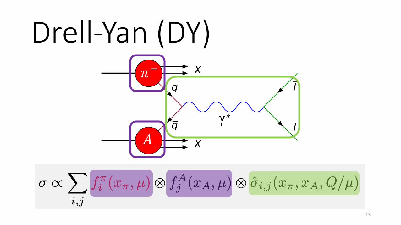
Drell-Yan (DY)𝜋!

𝐴

1313

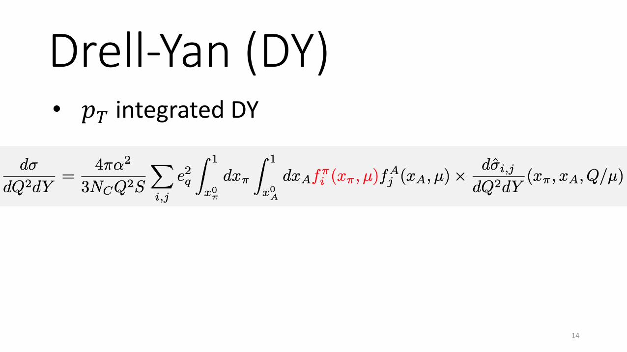
Drell-Yan (DY)

14

• 𝑝! integrated DY

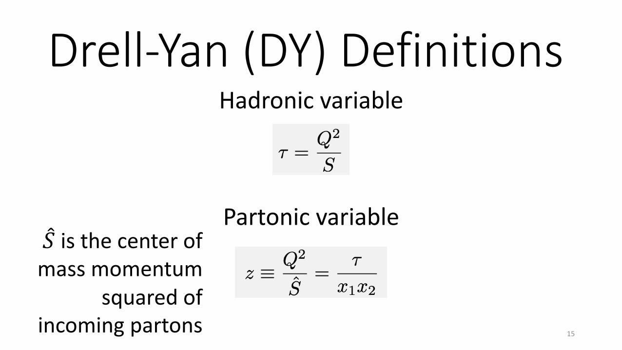
Drell-Yan (DY) DefinitionsHadronic variable

15

Partonic variable#𝑆 is the center of

mass momentum squared of

incoming partons

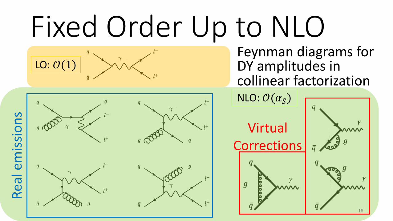
Fixed Order Up to NLOFeynman diagrams for DY amplitudes in collinear factorization

𝑞

#𝑞𝑔

𝛾

𝛾

𝛾

LO: 𝒪(1)

NLO: 𝒪(𝛼")

Real

em

issio

ns Virtual Corrections

16

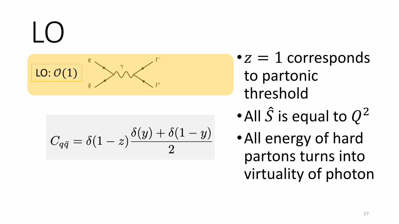
LOLO: 𝒪(1)

•𝑧 = 1 corresponds to partonic threshold•All %𝑆 is equal to 𝑄"

•All energy of hard partons turns into virtuality of photon

17

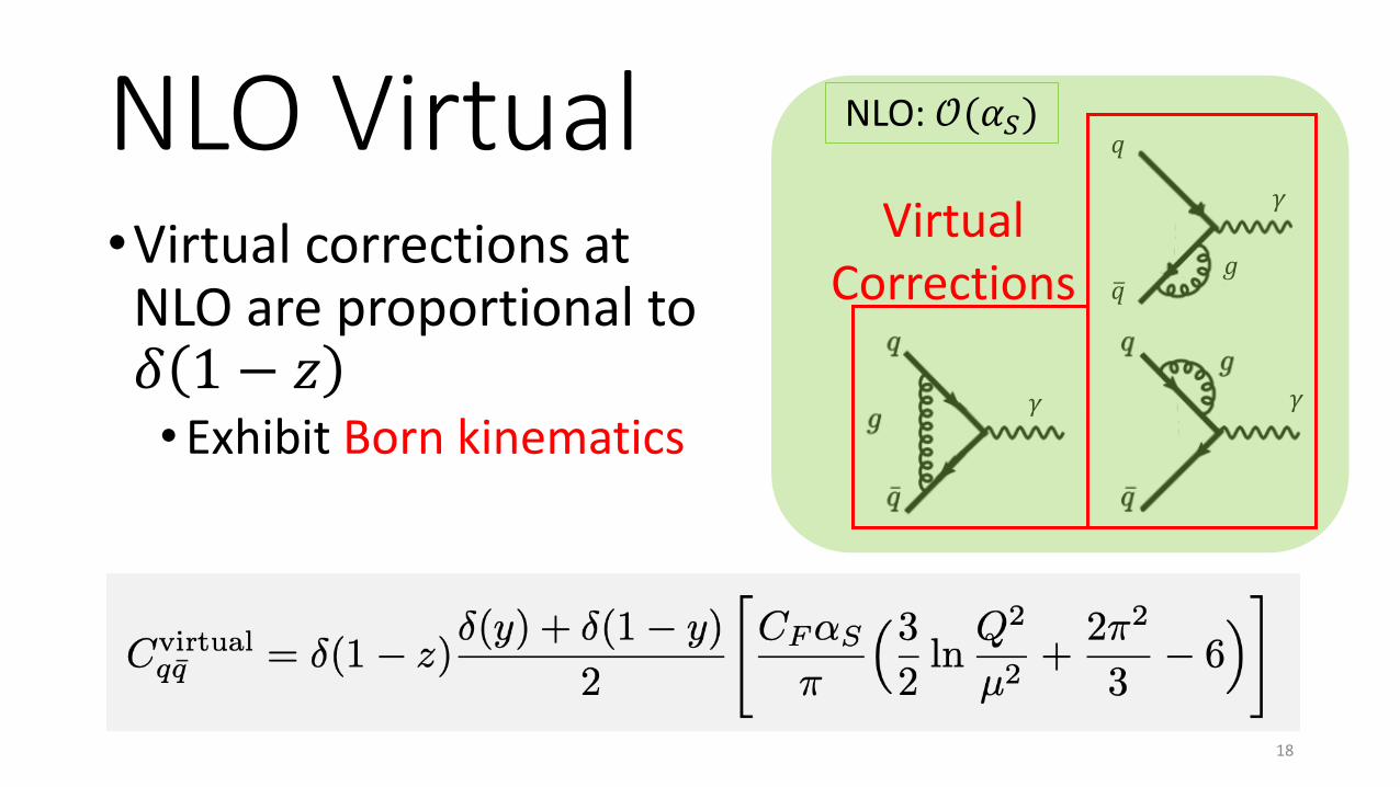
NLO Virtual 𝑞

#𝑞𝑔

𝛾

𝛾

𝛾

NLO: 𝒪(𝛼")

Virtual Corrections

•Virtual corrections at NLO are proportional to 𝛿 1 − 𝑧• Exhibit Born kinematics

18

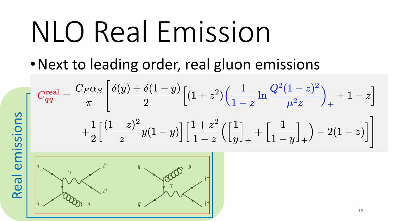
NLO Real EmissionRe

al e

miss

ions

•Next to leading order, real gluon emissions

19

NLO Real Emission•Plus distributions come from subtraction procedure of collinear singularities•When 𝑧 → 1, log(1 − 𝑧) can be large and potentially spoil perturbation•Appear in all orders in a predictable manner

20

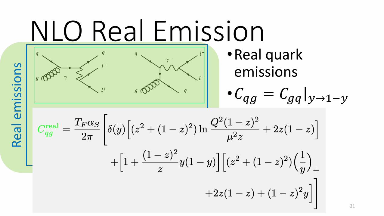
NLO Real EmissionRe

al e

miss

ions

•Real quark emissions•𝐶#$ = 𝐶$#|%→'(%

21

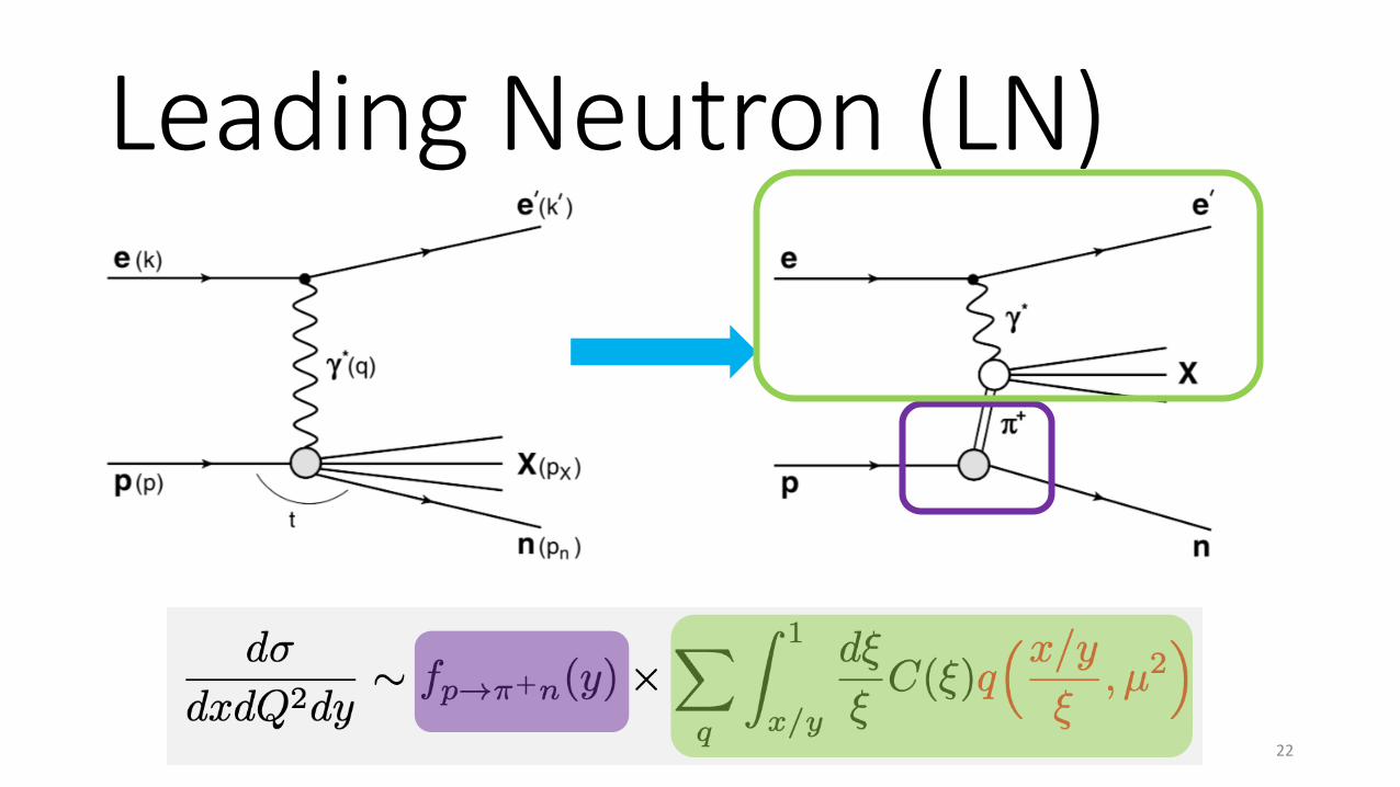
Leading Neutron (LN)

22

LN

•These data provide indirect measure of pion PDFs, since it is virtual•Need to have as small of |𝑡| as possible•Assumed dominance of 𝑡-channel exchange process by quantum numbers• Introduce some model dependence

23

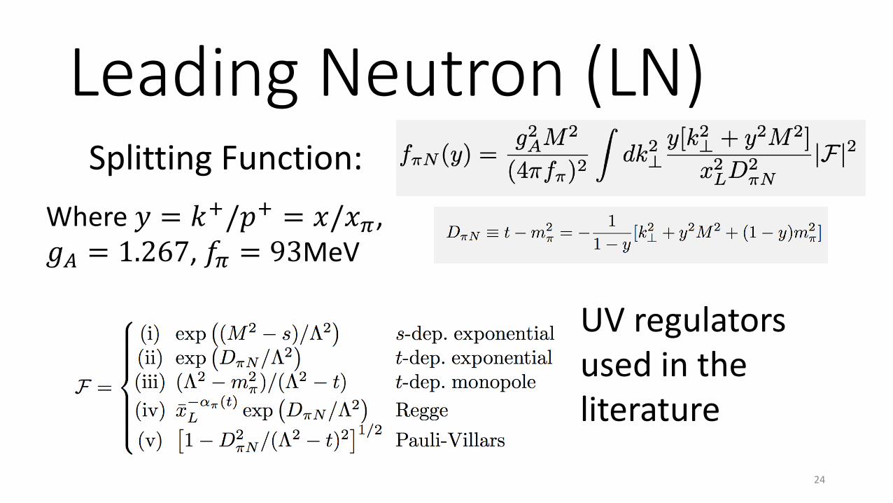
Leading Neutron (LN)Splitting Function:

Where 𝑦 = 𝑘!/𝑝! = 𝑥/𝑥", 𝑔# = 1.267, 𝑓" = 93MeV

UV regulators used in the literature

24

2a. DY-𝑞! Dependent Theory

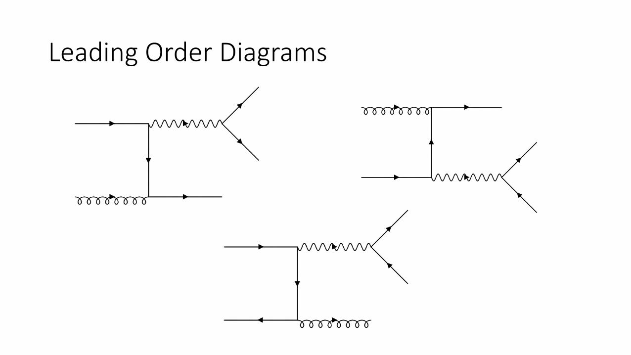
Leading Order Diagrams

Drell-Yan (DY)

27

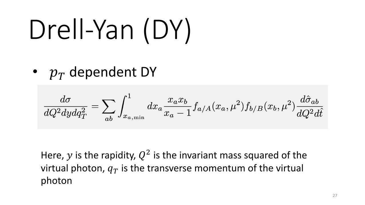
• 𝑝! dependent DY

Here, 𝑦 is the rapidity, 𝑄# is the invariant mass squared of the virtual photon, 𝑞! is the transverse momentum of the virtual photon

𝑞!-dependent DY definitions

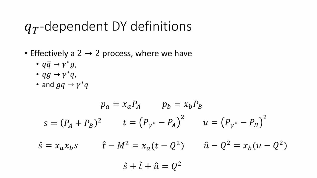
• Effectively a 2 → 2 process, where we have • 𝑞"𝑞 → 𝛾∗𝑔, • 𝑞𝑔 → 𝛾∗𝑞, • and 𝑔𝑞 → 𝛾∗𝑞

𝑝$ = 𝑥$𝑃% 𝑝& = 𝑥&𝑃'

𝑠 = 𝑃% + 𝑃' # 𝑡 = 𝑃(∗ − 𝑃%# 𝑢 = 𝑃(∗ − 𝑃'

#

�̂� = 𝑥$𝑥&𝑠 �̂� − 𝑀# = 𝑥$(𝑡 − 𝑄#) 6𝑢 − 𝑄# = 𝑥&(𝑢 − 𝑄#)

�̂� + �̂� + 6𝑢 = 𝑄#

𝑞!-dependent DY definitions

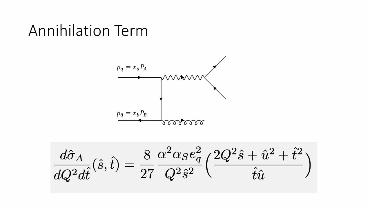
Annihilation Term

𝑝! = 𝑥"𝑃#

𝑝$! = 𝑥%𝑃&

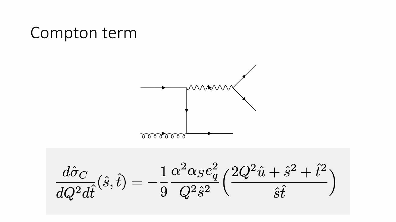
Compton term

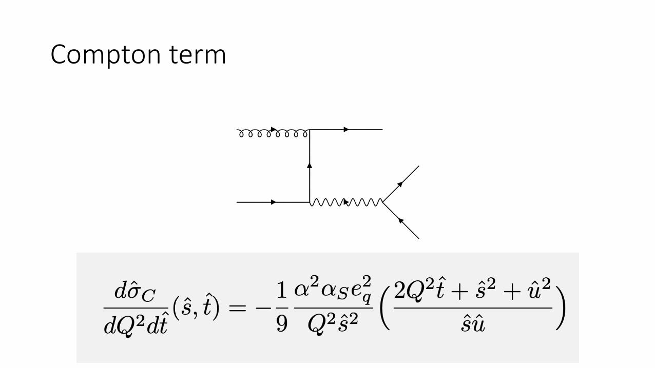
Compton term

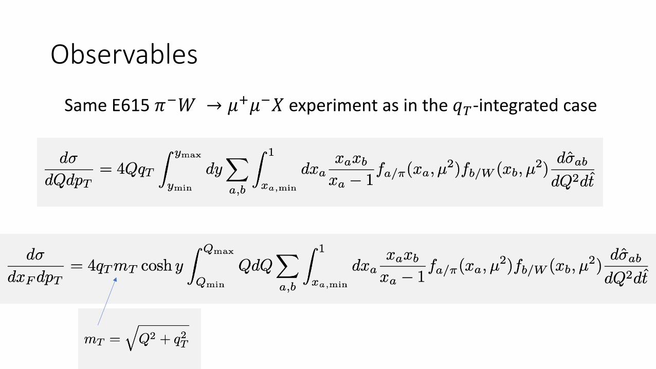
Observables

Same E615 𝜋)𝑊 → 𝜇*𝜇)𝑋 experiment as in the 𝑞!-integrated case

3. Fitting Methodology

Datasets

• We fit the PDFs to the following datasets• DY:• E615 – FNAL• NA10 – CERN

• LN:• H1 – HERA at DESY• ZEUS – HERA at DESY

• 𝑞!-dependent DY• E615 – FNAL (𝑄-dependent and 𝑥+-dependent)

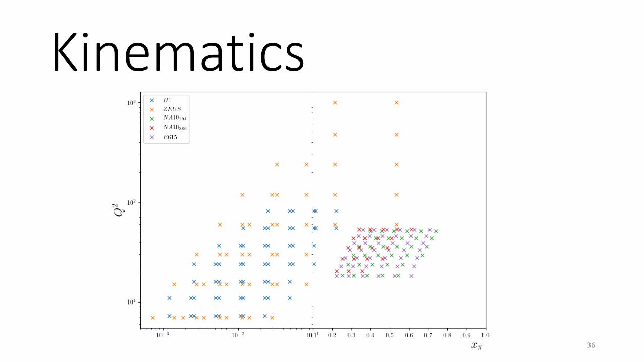
Kinematics

36

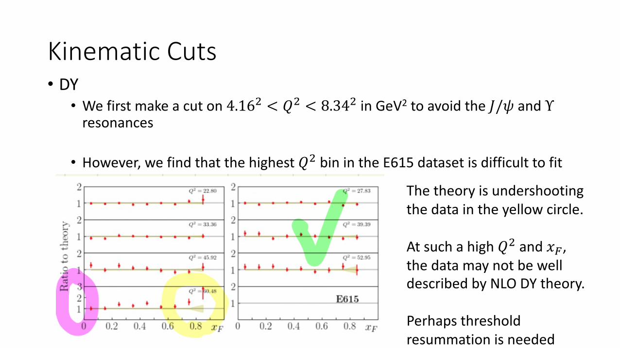
Kinematic Cuts• DY• We first make a cut on 4.16, < 𝑄, < 8.34, in GeV2 to avoid the 𝐽/𝜓 and Υ

resonances

• However, we find that the highest 𝑄, bin in the E615 dataset is difficult to fit

The theory is undershooting the data in the yellow circle.

At such a high 𝑄, and 𝑥+, the data may not be well described by NLO DY theory.

Perhaps threshold resummation is needed

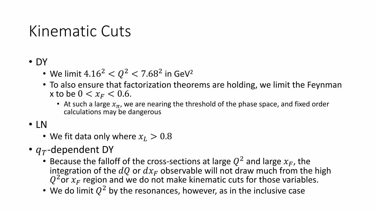
Kinematic Cuts

• DY• We limit 4.16, < 𝑄, < 7.68, in GeV2

• To also ensure that factorization theorems are holding, we limit the Feynman x to be 0 < 𝑥+ < 0.6.• At such a large 𝑥!, we are nearing the threshold of the phase space, and fixed order

calculations may be dangerous

• LN• We fit data only where 𝑥- > 0.8

• 𝑞!-dependent DY• Because the falloff of the cross-sections at large 𝑄, and large 𝑥+, the

integration of the 𝑑𝑄 or 𝑑𝑥+ observable will not draw much from the high 𝑄,or 𝑥+ region and we do not make kinematic cuts for those variables.• We do limit 𝑄, by the resonances, however, as in the inclusive case

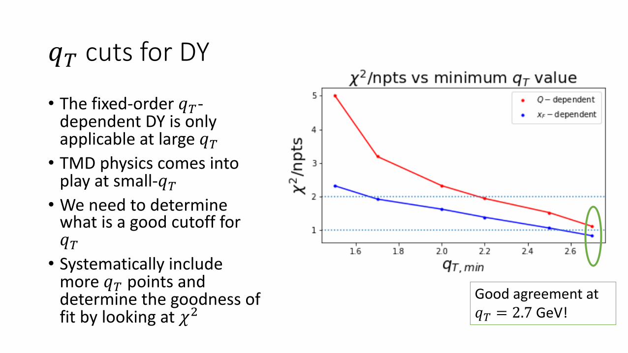
𝑞! cuts for DY

• The fixed-order 𝑞!-dependent DY is only applicable at large 𝑞!• TMD physics comes into

play at small-𝑞!• We need to determine

what is a good cutoff for 𝑞!• Systematically include

more 𝑞! points and determine the goodness of fit by looking at 𝜒#

Good agreement at 𝑞! = 2.7 GeV!

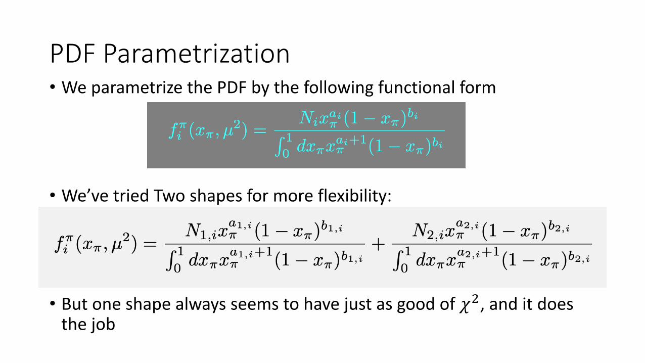
PDF Parametrization• We parametrize the PDF by the following functional form

• We’ve tried Two shapes for more flexibility:

• But one shape always seems to have just as good of 𝜒#, and it does the job

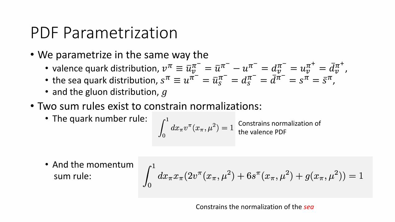
PDF Parametrization• We parametrize in the same way the• valence quark distribution, 𝑣. ≡ "𝑢/.

! = "𝑢.! − 𝑢.! = 𝑑/.! = 𝑢/.

" = �̅�/." ,

• the sea quark distribution, 𝑠. ≡ 𝑢.! = "𝑢0.! = 𝑑0.

! = �̅�.! = 𝑠. = �̅�., • and the gluon distribution, 𝑔

• Two sum rules exist to constrain normalizations:• The quark number rule:

• And the momentumsum rule:

Constrains normalization of the valence PDF

Constrains the normalization of the sea

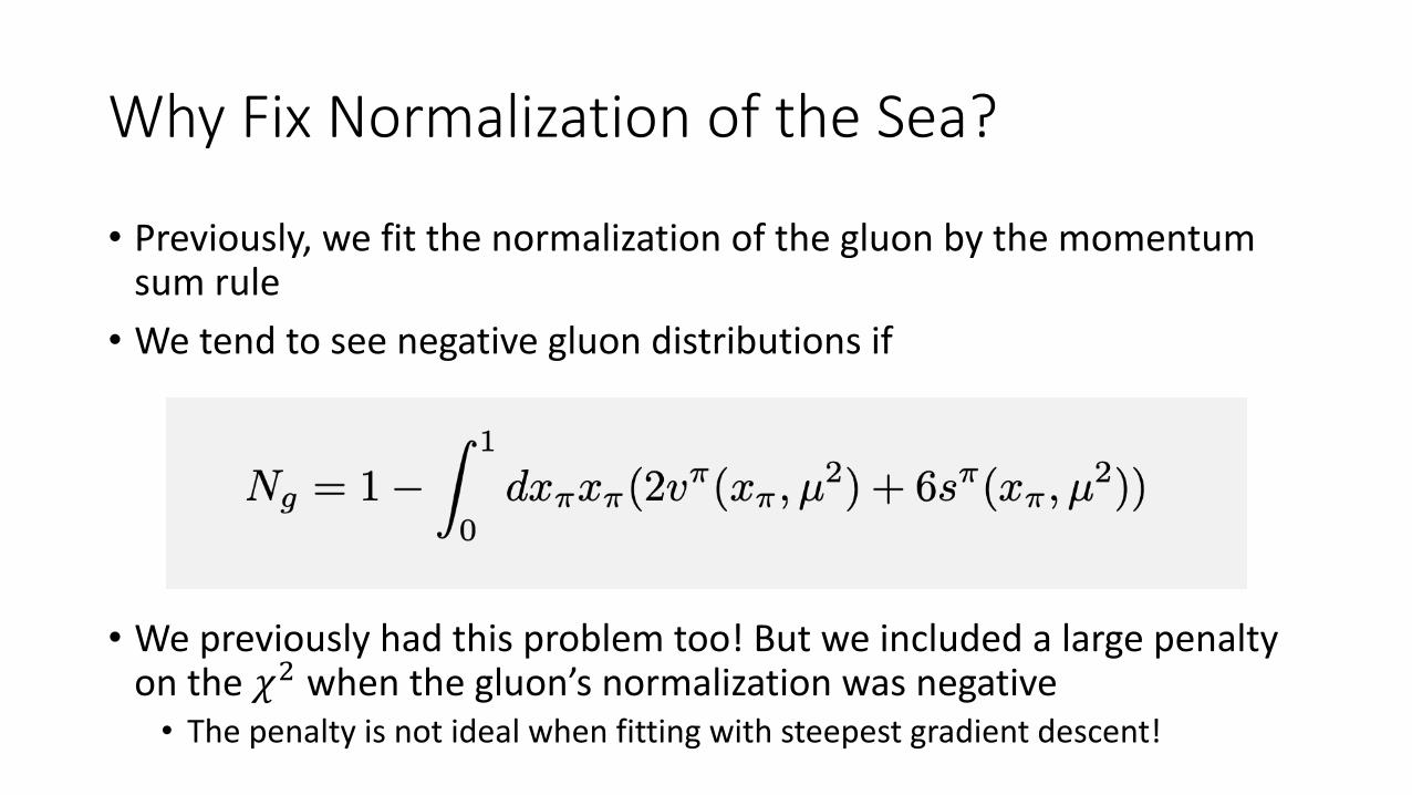
Why Fix Normalization of the Sea?

• Previously, we fit the normalization of the gluon by the momentum sum rule• We tend to see negative gluon distributions if

• We previously had this problem too! But we included a large penalty on the 𝜒# when the gluon’s normalization was negative• The penalty is not ideal when fitting with steepest gradient descent!

Fixing Normalization of the Sea

• We can more easily fix the normalization of the sea and hard-codethe normalization of the gluon to be a free parameter, but strictly positive• The sea never really becomes negative even though it is allowed to

Additional parameter constraints

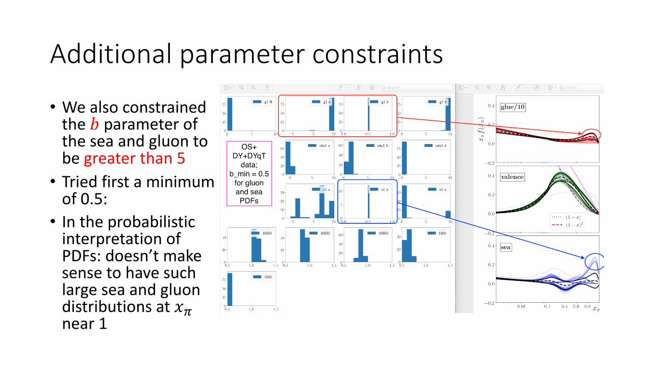
• We also constrained the 𝑏 parameter of the sea and gluon to be greater than 5• Tried first a minimum

of 0.5:• In the probabilistic

interpretation of PDFs: doesn’t make sense to have such large sea and gluon distributions at 𝑥!near 1

Bayesian Statistics

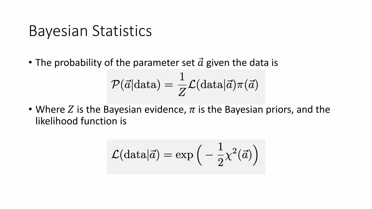
• The probability of the parameter set �⃗� given the data is

• Where 𝑍 is the Bayesian evidence, 𝜋 is the Bayesian priors, and the likelihood function is

Bayesian Statistics

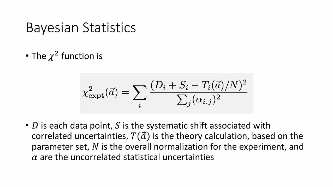
• The 𝜒# function is

• 𝐷 is each data point, 𝑆 is the systematic shift associated with correlated uncertainties, 𝑇(�⃗�) is the theory calculation, based on the parameter set, 𝑁 is the overall normalization for the experiment, and 𝛼 are the uncorrelated statistical uncertainties

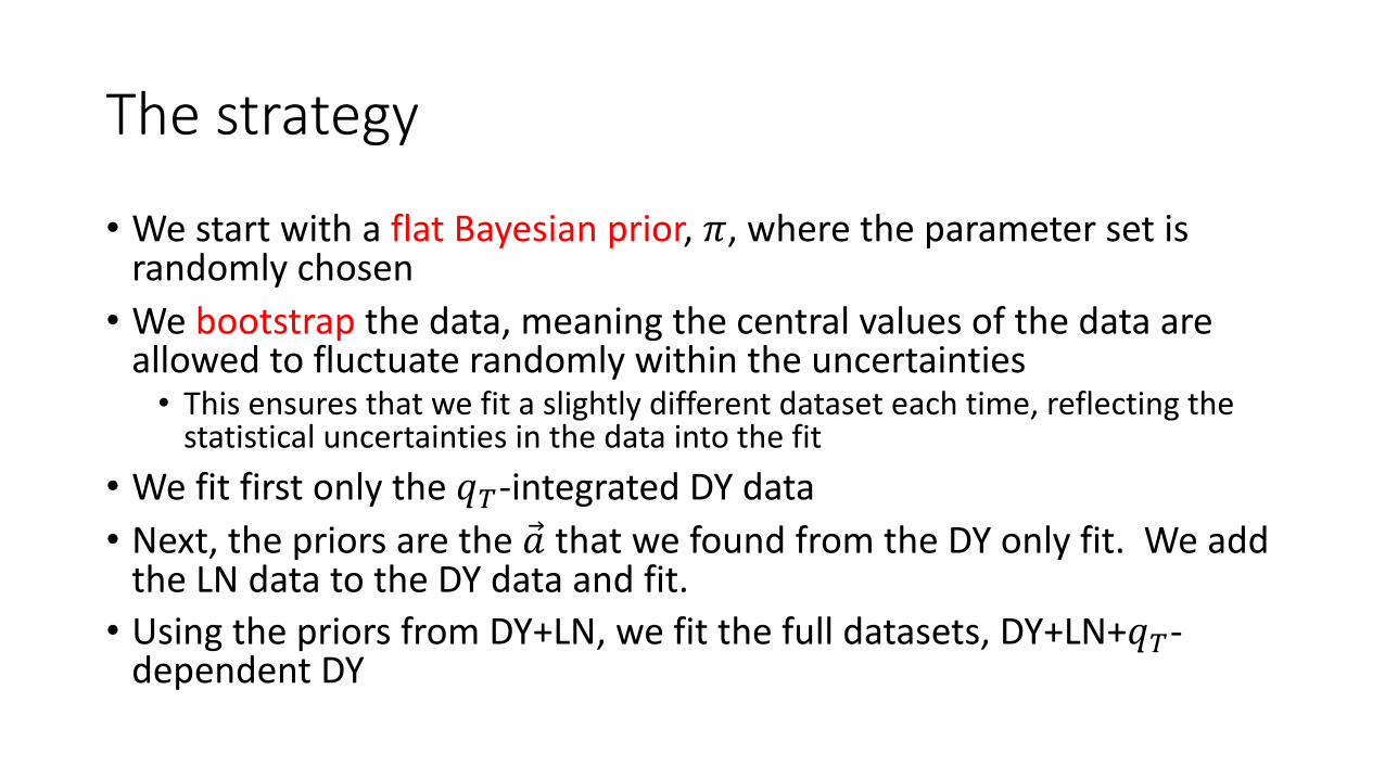
The strategy

• We start with a flat Bayesian prior, 𝜋, where the parameter set is randomly chosen• We bootstrap the data, meaning the central values of the data are

allowed to fluctuate randomly within the uncertainties• This ensures that we fit a slightly different dataset each time, reflecting the

statistical uncertainties in the data into the fit• We fit first only the 𝑞!-integrated DY data• Next, the priors are the �⃗� that we found from the DY only fit. We add

the LN data to the DY data and fit.• Using the priors from DY+LN, we fit the full datasets, DY+LN+𝑞!-

dependent DY

4. Results

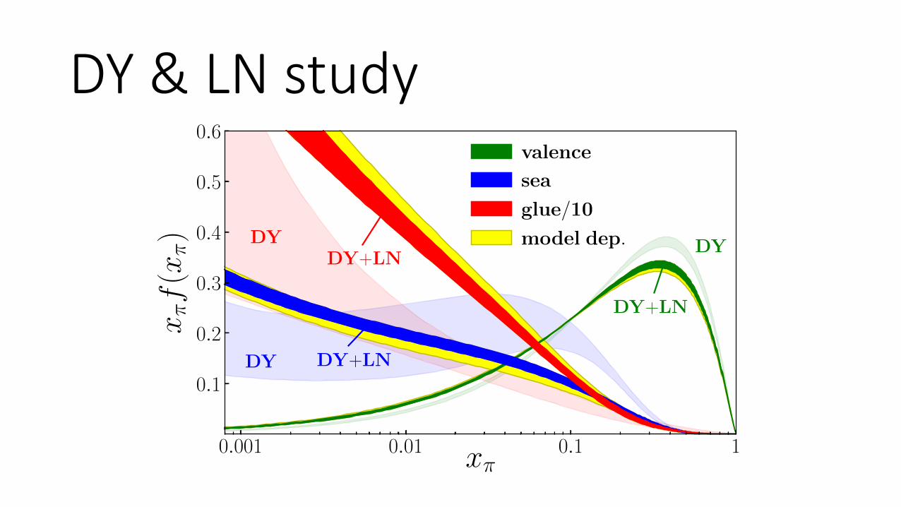
DY & LN study

0.001 0.01 0.1 1xº

0.1

0.2

0.3

0.4

0.5

0.6

xºf(x

º) DY

DY+LN

DY DY+LN

DYDY+LN

valence

sea

glue/10

model dep.

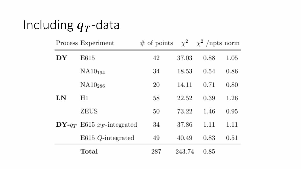
Including 𝑞!-data

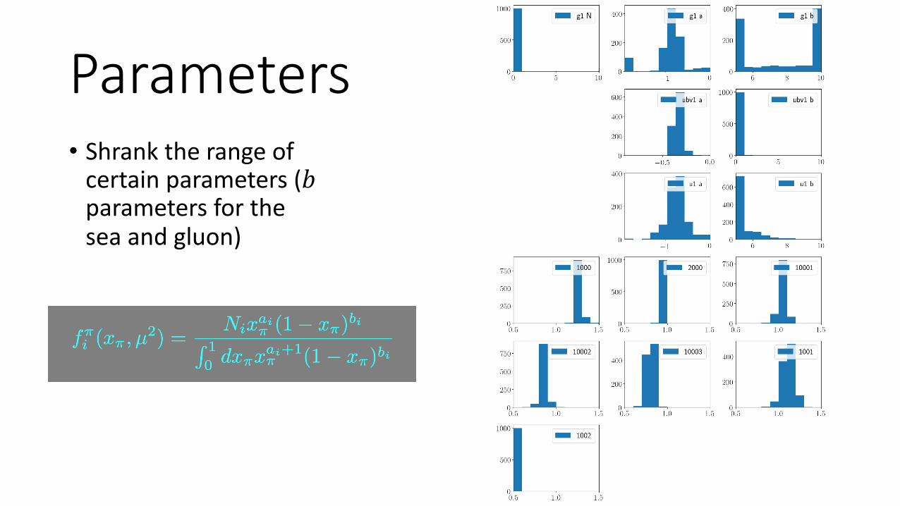
Parameters• Shrank the range of

certain parameters (𝑏parameters for the sea and gluon)

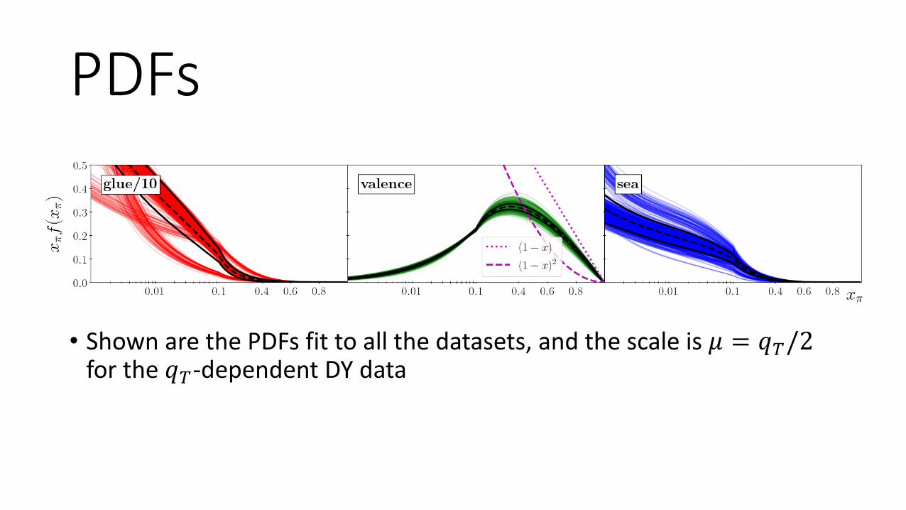
PDFs

• Shown are the PDFs fit to all the datasets, and the scale is 𝜇 = 𝑞!/2for the 𝑞!-dependent DY data

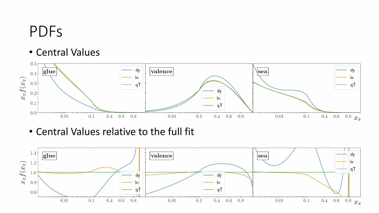
PDFs• Central Values

• Central Values relative to the full fit

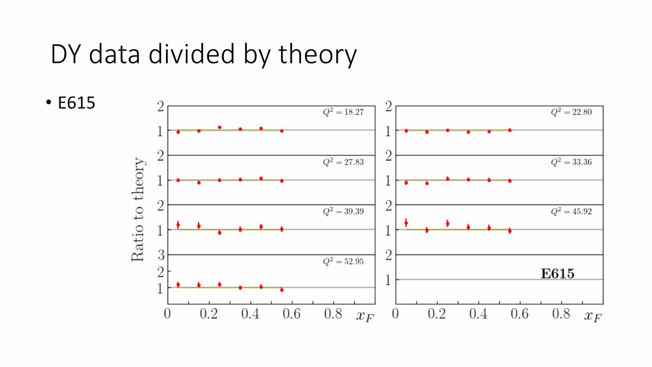
DY data divided by theory• E615

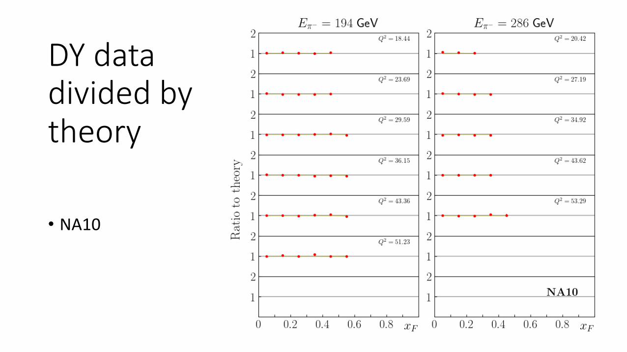
DY data divided by theory

• NA10

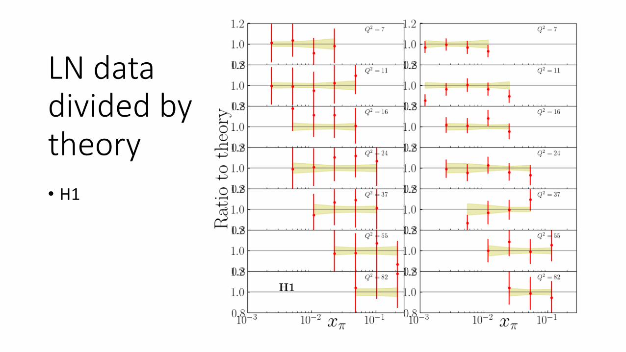
LN data divided by theory• H1

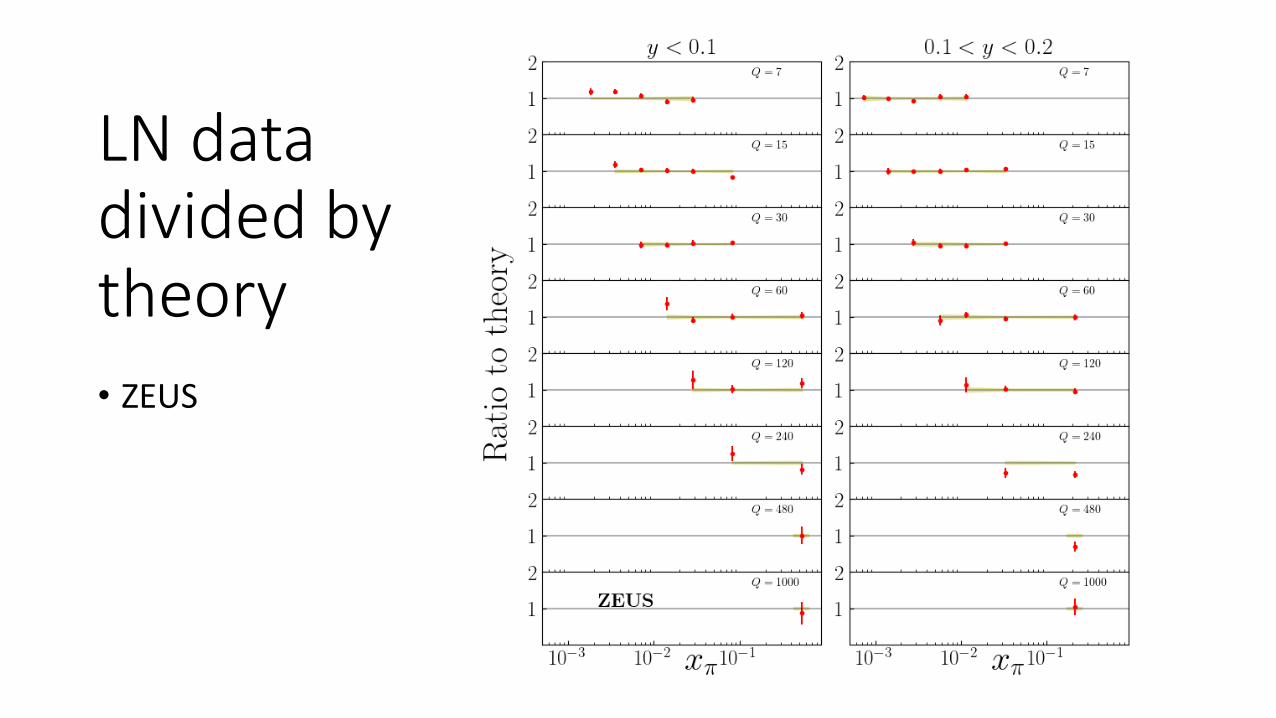
LN data divided by theory• ZEUS

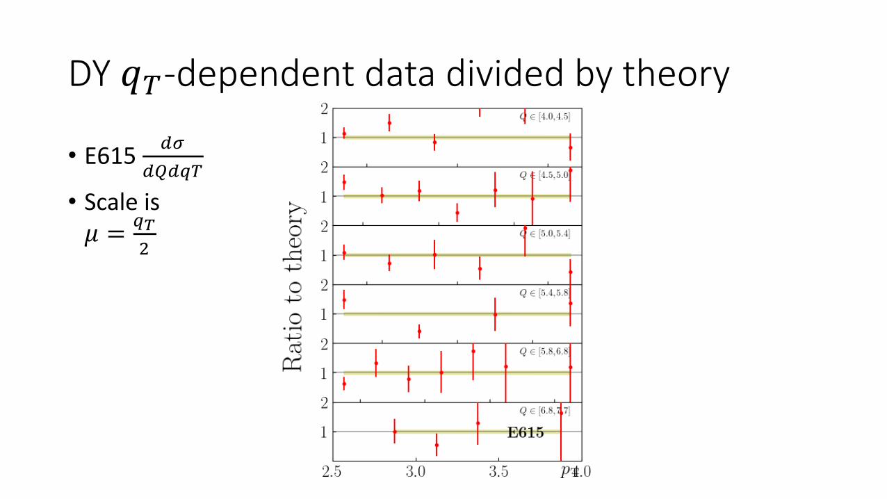
DY 𝑞!-dependent data divided by theory

• E615 ,-,.,/!

• Scale is 𝜇 = /"

#

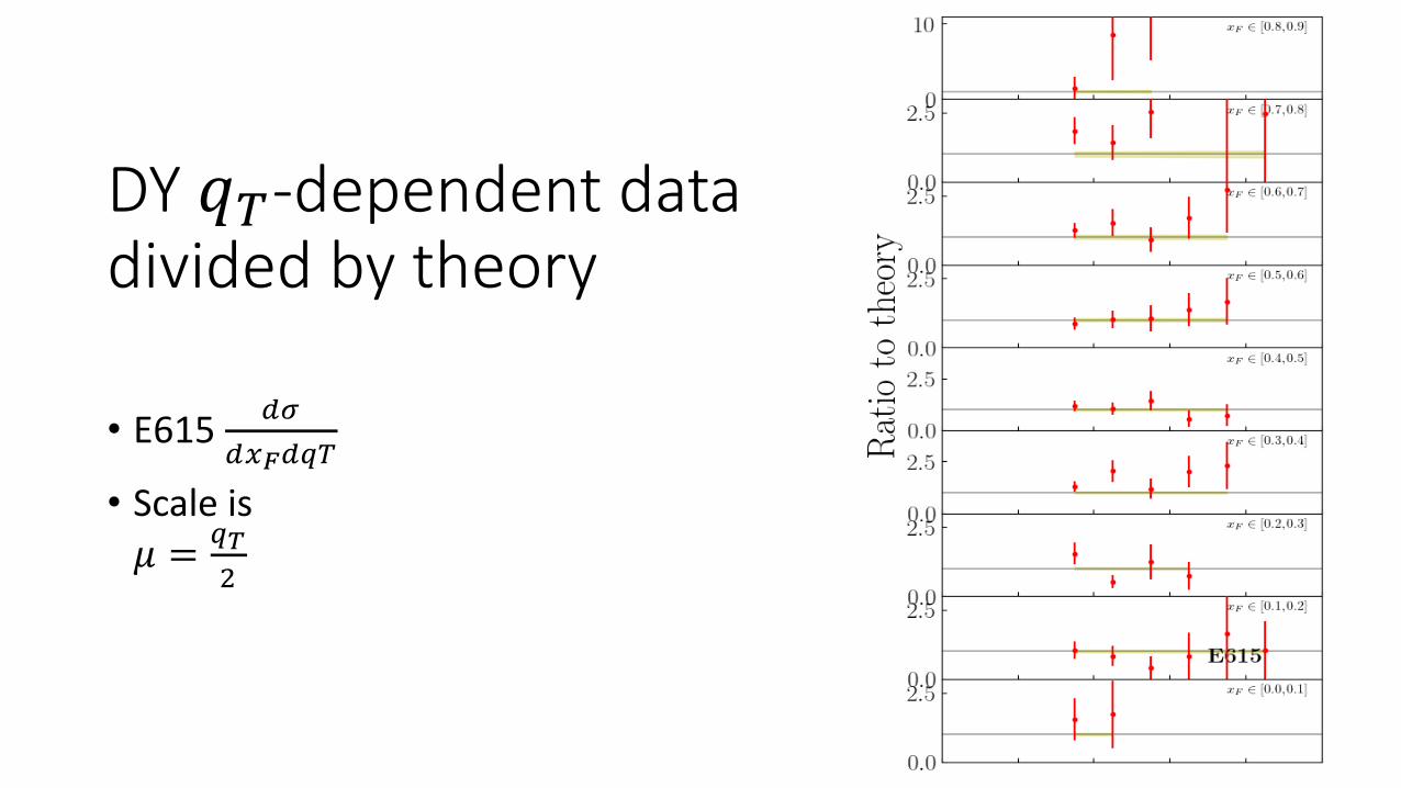
DY 𝑞!-dependent data divided by theory

• E615 ,-,0#,/!

• Scale is 𝜇 = /"

#

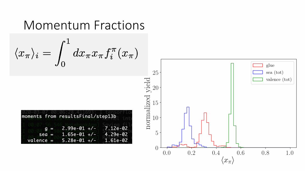
Momentum Fractions

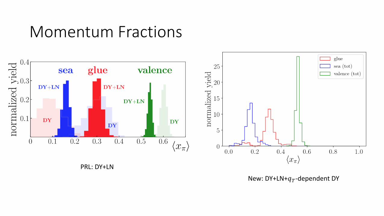
Momentum Fractions

PRL: DY+LN

New: DY+LN+𝑞'-dependent DY

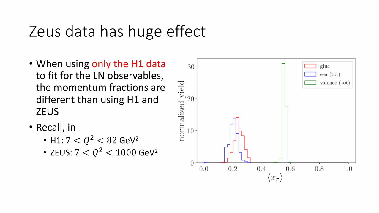
Zeus data has huge effect

• When using only the H1 data to fit for the LN observables, the momentum fractions are different than using H1 and ZEUS• Recall, in • H1: 7 < 𝑄, < 82 GeV2

• ZEUS: 7 < 𝑄, < 1000 GeV2

5. Impact of 𝑞!-dependent DY

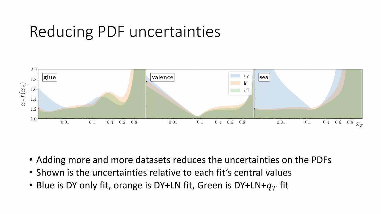
Reducing PDF uncertainties

• Adding more and more datasets reduces the uncertainties on the PDFs• Shown is the uncertainties relative to each fit’s central values• Blue is DY only fit, orange is DY+LN fit, Green is DY+LN+𝑞" fit

Channel-by-channel contribution

• We can see the observables of each experiment in terms of the degrees of freedom that we fit, i.e. valence, sea, and gluon PDFs• The larger the contribution to the overall cross-section means the

more constraints come from that observable

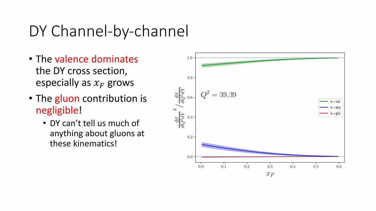
DY Channel-by-channel• The valence dominates

the DY cross section, especially as 𝑥1 grows• The gluon contribution is

negligible!• DY can’t tell us much of

anything about gluons at these kinematics!

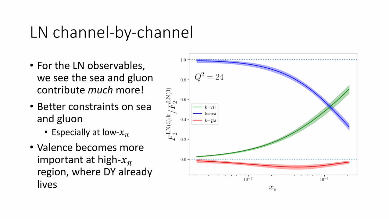
LN channel-by-channel

• For the LN observables, we see the sea and gluon contribute much more!• Better constraints on sea

and gluon• Especially at low-𝑥.

• Valence becomes more important at high-𝑥2region, where DY already lives

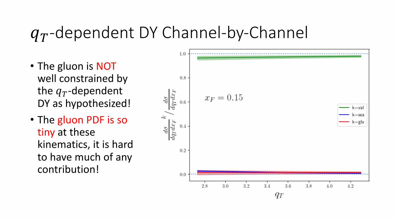
𝑞!-dependent DY Channel-by-Channel

• The gluon is NOT well constrained by the 𝑞!-dependent DY as hypothesized!• The gluon PDF is so

tiny at these kinematics, it is hard to have much of any contribution!

6. Scale Dependence

Ambiguity of Scale

• In Collinear Factorization, one needs a hard scale that is 𝜇 ≫ Λ, where 𝜇 is a hard, partonic scale, and Λ is a scale associated with soft, non-perturbative physics• In DIS, for instance, one hard scale exists, 𝑄#, which is the invariant

mass of the virtual photon• In DY, again, only one hard scale exists, 𝑄#

• However, in the 𝑞!-dependent DY, two scales exist• The invariant mass of the dilepton pair, 𝑄, is measured, but also the

transverse momentum of the dilepton pair, 𝑝!• Which scale is appropriate?

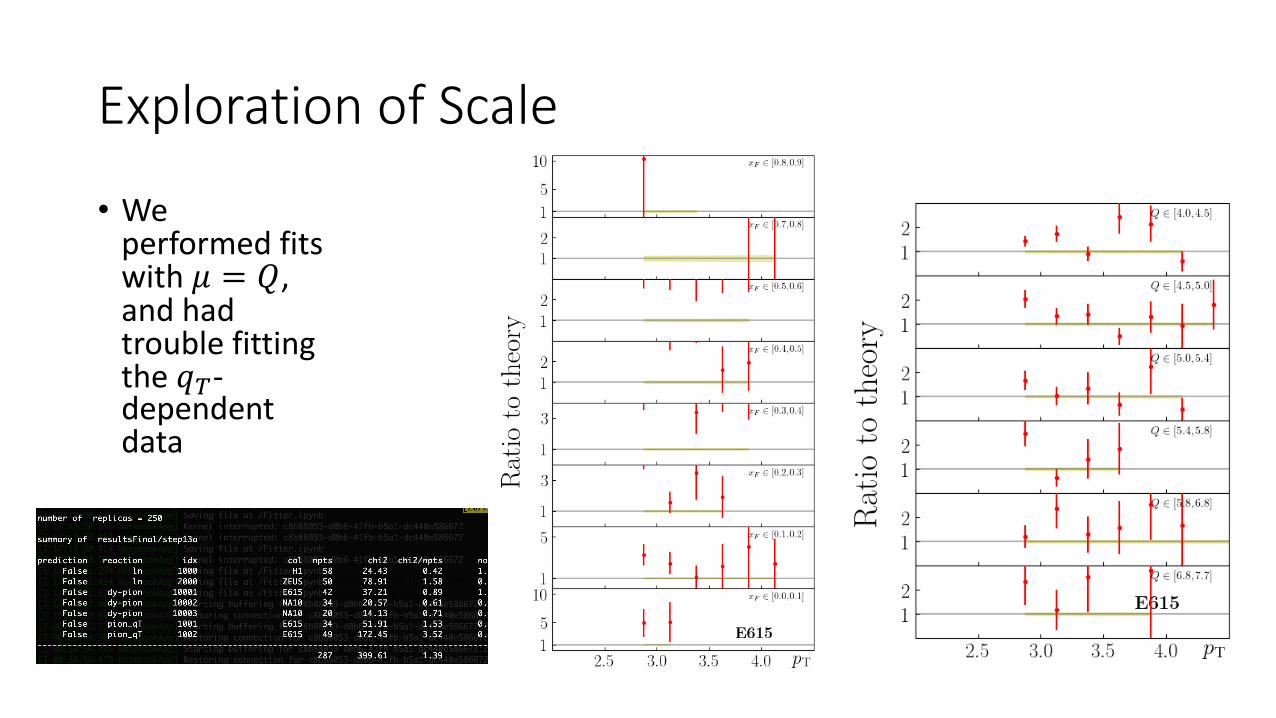
Exploration of Scale

• We performed fits with 𝜇 = 𝑄, and had trouble fitting the 𝑞"-dependent data

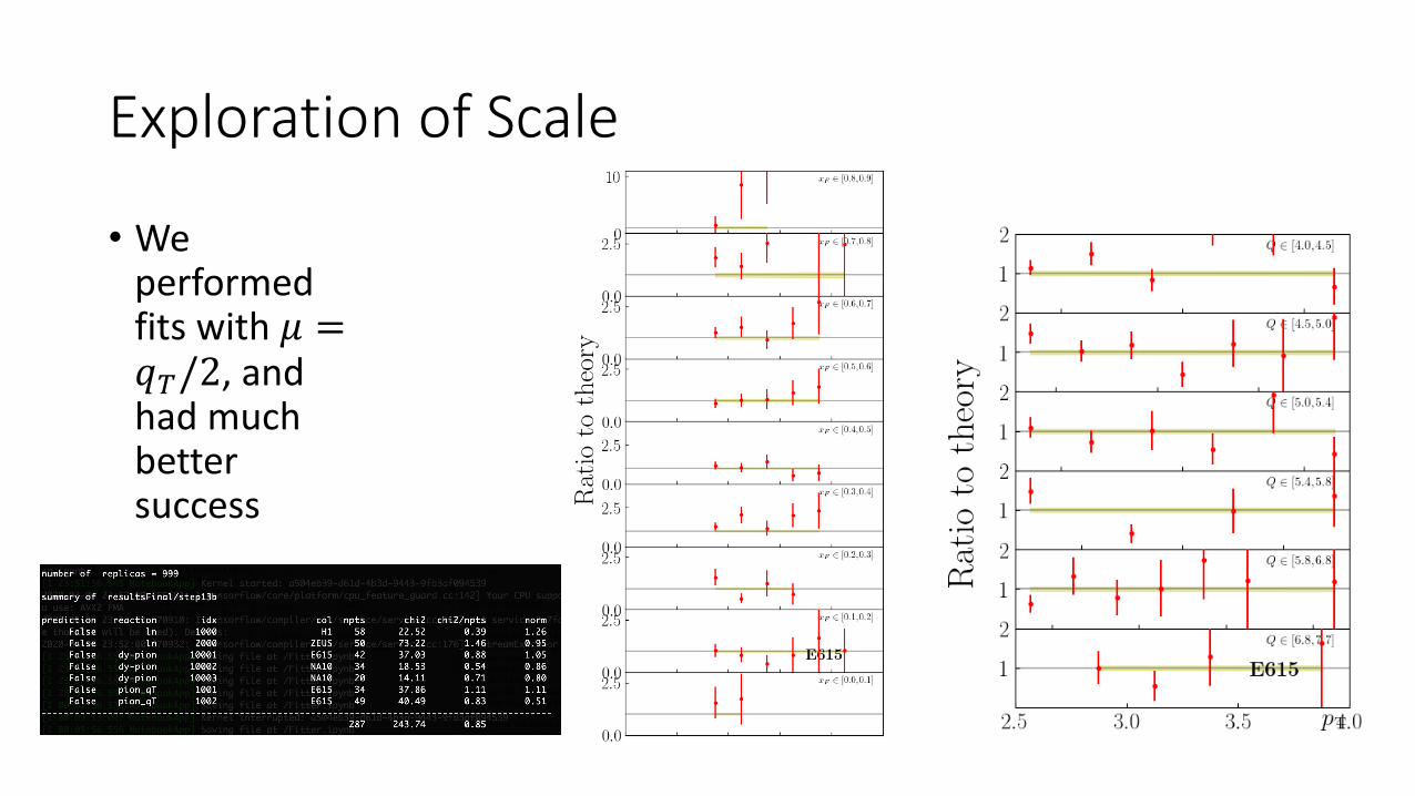
Exploration of Scale

• We performed fits with 𝜇 =𝑞!/2, and had much better success

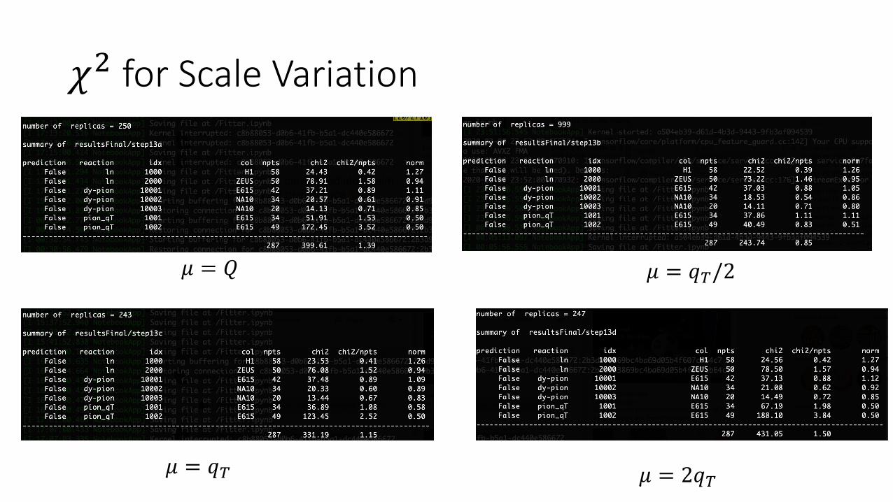
𝜒1 for Scale Variation

𝜇 = 𝑄 𝜇 = 𝑞!/2

𝜇 = 𝑞! 𝜇 = 2𝑞!

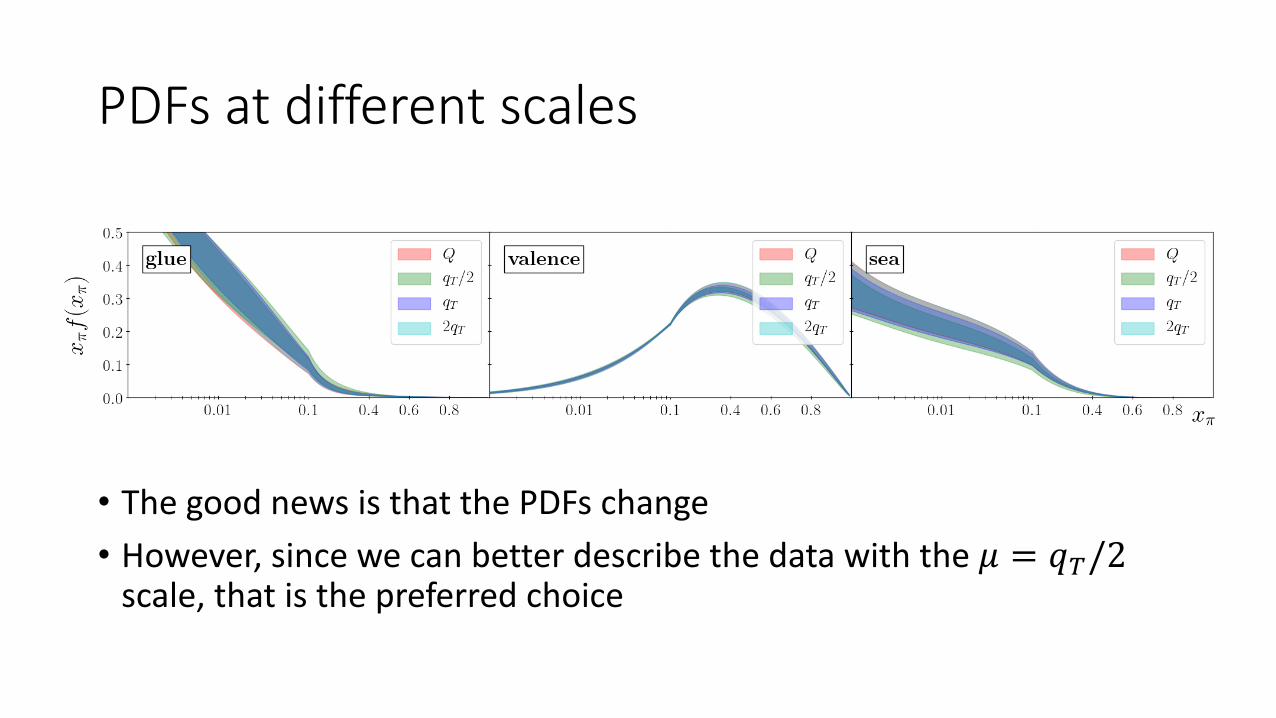
PDFs at different scales

• The good news is that the PDFs change• However, since we can better describe the data with the 𝜇 = 𝑞!/2

scale, that is the preferred choice

7. Future Work

This Analysis•Put PDFs on LHAPDF for community use•Compare the proton vs pion•Make projections for EIC kinematics

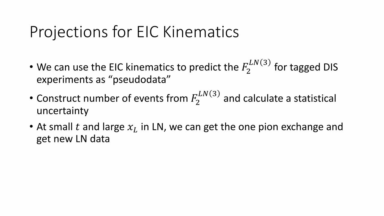
Projections for EIC Kinematics

• We can use the EIC kinematics to predict the 𝐹#34 5 for tagged DIS

experiments as “pseudodata”

• Construct number of events from 𝐹#34 5 and calculate a statistical

uncertainty• At small 𝑡 and large 𝑥3 in LN, we can get the one pion exchange and

get new LN data

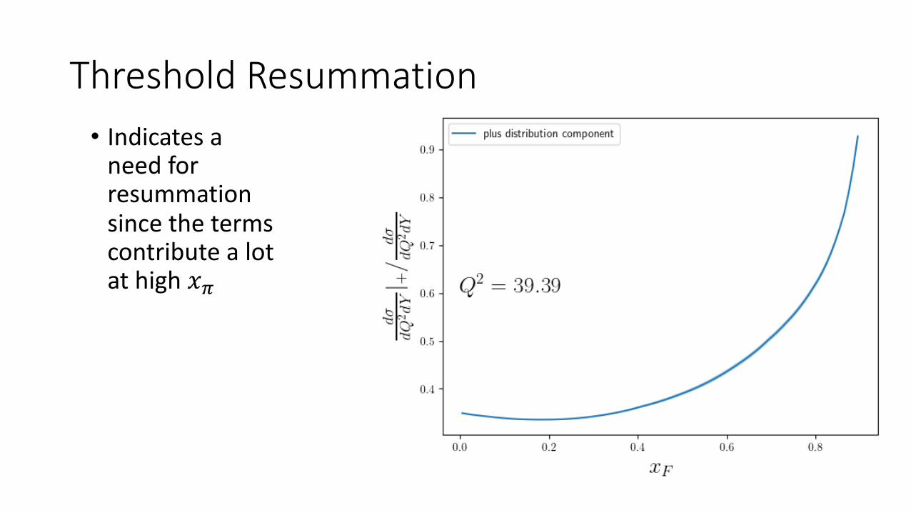
Threshold Resummation• Indicates a

need for resummationsince the terms contribute a lot at high 𝑥2

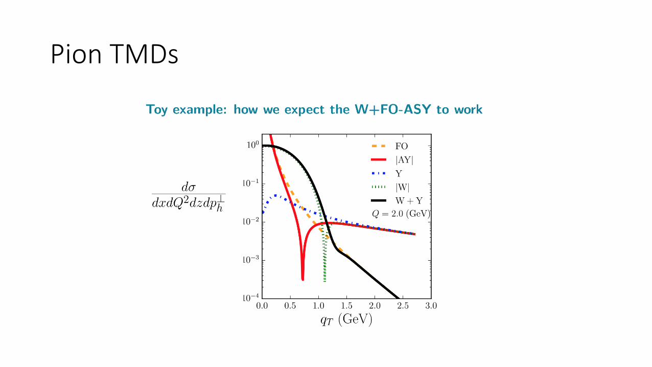
Pion TMDs