Impact of Efficiency gain under Competitive Pressure on Indian

Households: A General Equilibrium Approach

Amarendra Sahoo CenTER, University of Tilburg, The Netherlands

Jel: D57, D58, D33, D61, O40, I3 Abstract: The study makes an attempt to look into the question how competitive pressure would impact upon the income distribution and poverty of household groups through the change in productivity-efficiency in the economy using an input-output analysis in a general equilibrium framework. We consider three sources of growth: efficient utilization of available resources, technical progress and gain from terms of trade by re-orientation of trade. Welfare maximization under competitive spirit has resulted in efficiency gain, but at the cost of adverse income distribution. Rural household groups suffer more than the urban ones. It is noticed that change in income at the optimal allocation is the dominant factor in affecting household poverty. Urban households also enjoy significantly more reduction in poverty than the rural households. In fact, some of the rural households, involved in agricultural wage activity, suffer from increase in poverty. When capital is allowed to mobile across the sectors, there is higher gain in productivity and higher income disparity vis-à-vis the sector-specific capital. But, poverty effect is better, though marginally; in case capital is sector specific than mobile. The study shows that competitive pressure has positive effect on productivity-efficiency and poverty, but adverse effect on income distribution in Indian economy.

1

Impact of Efficiency gain under Competitive Pressure on Indian Households: A General Equilibrium Approach

1. Introduction

Economists and policy makers are always concerned about the economic growth, income

distribution and poverty of a low-income economy like India. Various studies have highlighted

that growth of the economy can affect the poor and income distribution some way or other.

Having faced with the unprecedented economic crisis in the beginning of 1990s, Indian

economic resorted to major reform program in July 1991. With a view to improving the

efficiency, productivity and global competitiveness, both macro and microeconomic reforms

were introduced in industrial, trade and financial policies (Bhagwati and Srinivasan, 1993).

Indian economy seemed to be responsive to the reform measures undertaken during 1991-96

with considerable globalisation and liberalisation. The GDP growth was more than 6.5 percent

per annum during this period. However, many reform commentators believe that a still lot

remains on India’s unfinished agenda (Bajpai and Sachs, 1997). A greater momentum of reform

is necessary with more openness in trade, deregulation of industries, agricultural reforms in

prices and trade, labour market reform (Fischer, 2002). It is expected that the renewal of

momentum in ongoing reform process would inspire the economy into a competitive

environment, where efficient reallocation of resources would result in gain in productivity level

and activities of the economy would operate on the frontier. Once the economy operates on the

frontier, the, the resultant competitive rewards to factors would force the households to re-

adjustment of their consumption and income, which would indicate heterogeneous impact on

the welfare distribution of households in the economy.

For last couple of decades, a lot of research has gone into the issue of growth- to- inequality

causality in the tradition of Kaldor (1956) and Kuznets (1955), which discuss the hypotheses

that growth could create or absorb inequality (Papanek and Kyn, 1986, Fields, 1991, Cogneau

and Guenard, 2002). Economic growth is the main source of creating income and employment

opportunity. With the economic growth, market for different goods in which different

households are engaged, expands which results in extended employment opportunities and

hence, change in income distribution. For India, major policy changes took place in the

beginning of 1990's. Biggest challenge of India's economic reforms programme has been

liberalisation of different sectors, e.g. trade and industry. In the pre-1990s, for long, Indian

industries were characterized by inefficiency, high costs and uneconomical means of

2

production with pervasive government control. To make Indian economy more competitive,

policy makers are still struggling with the idea to keep the distortion and restriction on trade

and industry to the minimum possible level. Though macro implications of the these reforms

are important, their impacts at the household level are not analysed well, which are of great

concern to any society. Given the heterogeneity of population and household groups, effects of

competition on their income distribution and welfare are not expected to be uniform. Further,

though India has an impressive record of growth since late 1980s, it still faces massive

challenges of poverty and inequality. Many studies, viz. Kawani and Subbarao (1990), Jain and

Tendulkar (1990), Datt and Ravallion (1992), and Ravallion and Datt (1996), have emphasised

the dominating influence of growth on poverty in India. This paper makes an attempt to look

into the question how competitive pressure with free trade would impact upon the income

distribution and poverty of household groups through the change in productivity-efficiency in

the economy using an input-output analysis in a general equilibrium framework.

Productivity of an economy depends on the maximum value added generated by proper

utilization of given amount of factors of production, e.g. land, labour and capital. If the

economy is competitive, all the economic agents maximize their objective function and the

economy is supposed to function on the production possibility frontier with competitive prices.

Hence, both first welfare theorem, i.e. commodity bundle generated by the equilibrium price

vector is efficient, and the second welfare theorem, i.e. an efficient allocation is equilibrium,

are fulfilled (ten Raa, 2002). As it is believed that Indian economy is not yet perfectly

competitive, the resource allocation in the economy is not yet optimal and hence, below the

production possibility frontier. The inefficiency is measured by the degree by which the net

output vector could be extended until it reaches the production frontier (ten Raa, 1995). Despite

many sceptical views on free trade versus growth (Rodriguez and Rodrik, 1999; Rodrik, 1999),

there has been strong evidence that free trade is growth enhancing (Sachs and Warner, 1995;

Edwards, 1992). Some of the heavyweights in trade and development economics have strongly

reiterated in their theoretical expositions that in the absence of market failure and distortions,

trade is welfare-improving growth (Bhagwati, 1994; Srinivasan and Bhagawati, 1999). Our

basic model is drawn heavily from ten Raa and Mohnen (2002). The growth of total factor

productivity (TFP) is captured by more efficient utilization of resources (Debreu, 1951) as well

as by technological change (Solow, 1957). The incorporation of input-output (I-O) framework

in this model allows for capturing intersectoral linkages and provides technological change of

TFP. However, unlike Solow residual, which is based on observable value share due to the

3

inherent assumption of competitive economy, the model used shadow prices of the output and

input derived from frontier program in the general equilibrium framework. Consumer

preferences are maximized given the constraint on technology and endowments of primary

endowment (trade surplus is also considered to be endowment of the economy). The model is

based on the fundamentals of the economies, where both the welfare theorems are satisfied.

This above theory could explain that the economy without trade can make use of the available

set, i.e. vectors of goods and services available for final use to operate on production possibility

curve. But by using gainful trade to exchange goods and services produced at home for those

produced abroad, the economy could add to its availability set under autarky (Srinivasan and

Bhagwati, 1999). In their theoretical exposition they explained that under the neoclassical

assumptions of complete market structure and minimal government intervention, a competitive

equilibrium under free trade is Pareto Optimum, where an economy will be productively

efficient (on its production possibility frontier) and also distributionally efficient (on utility

possibility frontier).

In a small open economy framework using the above technique, ten Raa and Mohnen (2001)

have shown the location of comparative advantages between Canada and Europe. Using I-O

tables from 1962 to 1991, ten Raa and Mohnen (2002) tried to capture the shift of source of

productivity growth from technical change to terms of trade effect. In all their studies, they

endogenize internal prices, while keeping the international prices exogenous. In the similar line,

with a new technological change measure, Shestalova (2002) has analyzed the TFP

performance of three large trading economies, viz. US, Japan and Europe. Both internal as well

as international prices are endogenized in her model. However, all the above models have not

focused on the change in personal income under perfect competition. ten Raa and Pan (2002)

have dealt with this issue for China. They divide China into 30 I-O sectors and 27 provinces.

This study shows that competition leads to losers and winners, both in terms of factor claims

and in terms of regions. Their input-output table divides factor of production of labour, i.e.

factor income of labour into different categories according to skill. Both Shestalova(2002) and

Raa and Paan (2002) have used differential optimum regional trade surpluses against the actual

ones as an adjustment process to get final adjusted weights of individual preferences.

A significant difference of our model from similar above-mentioned models is that in our

model, differential household propensity to consume plays an important role in readjustment of

consumption-income at the optimum. This is because, if the household’s propensity to consume

4

at the optimum exceeds benchmark propensity to consume more than the other household, then

the general equilibrium welfare maximization requires that former household should be

assigned with higher consumption share than the later. The weights attached to the household

preferences in our model are adjusted not using differential optimal trade surpluses, but keeping

the ratio of optimum propensity to consume to the observed one same for all the household

groups. Moreover, our income and consumption pattern will be evaluated for different

household categories on the basis of an extended I-O table, i.e. social accounting matrix

(SAM), based on household share of endowment of different factors. The nice thing about

using SAM in our model is that it captures the sources of income for different household

groups, i.e. ownership of factor endowments, and expenditure pattern of different household

groups. The model deals with only one economy for one period. We consider small country

assumption, where tradable sectors are price takers.

The rest of the paper is divided into five sections. The theoretical model is highlighted in the

Section 2. Section 3 analyses the basic data set and Section4 briefly describes the

endogenisation of poverty and measure inequality in our framework. Results and implications

of the model are discussed in the Section 5, while Section 6 gives the conclusion to the paper.

2. The Methodology

The analysis has been conducted using the benchmark data set for 1994-95. The model includes

21 production sectors and 9 household groups defined on the basis of income classes. There are

four rural and five urban household groups. Households have welfare function of the Leonteif

type1, that is, the vector of consumption demand describes the household preference.

Considering an open economy, we endogenize the net exports, i.e. the trade deficit, in the

model. The balance of payment controls the net exports. Capital, land, labour and trade deficit

are considered to be endowment in the economy. In the model, each household group has

consumption demand vector, fhdhD, where D can be interpreted as the expansion factor for the

weighted sum of the private consumption demands of the nine household groups, fh is the

vector of consumption shares of commodities and dh represents consumption weights attached

to the household groups. Model maximizes total welfare of the economy by maximizing total

final private consumption subject to commodity, factor and trade deficit constraints keeping the

1 Concavity of individual utility functions should be assumed in order to preserve the concavity of the aggregate of these functions.

5

relative composition of the vector of private consumption demand each household group fixed.

Rest of the final demand, which includes government consumption and investment, is fixed in

the model2. The shadow prices reflect the commodity prices and factor prices of labour, capital

and land. These optimum prices are applied to derive the income and expenditure of different

household groups. In the general equilibrium setting, we want to keep the ratio computed new

propensity to consume to the observed one same across all the household groups. The solution

yields new set of consumption weight for each household. The allocations of activity and

shadow prices that are finally obtained constitute the general equilibrium. Our model captures

characteristics of Negishi format of welfare optimum (Negishi, 1960)3.

It is obvious that given small country assumption and no trade distortion, if all sectors are

assumed to be tradable, then competitive pressure seems to have no impact on the income

distribution, though efficiency of the economy might change. In this case, even though the

frontier of the economy moves, the prices of, both output and factor, remain same as

benchmark (see Appendix II)4. In the extreme case of closed economy, as factors and

productions are adjusted inside the economy, there is scope for prices and consumption-weights

to change at the optimum. However, we take more realistic case for Indian economy with 19

tradable and 2 non-tradable sectors.

The frontier of the economy is the maximum expansion of its total final demand with relative

composition of consumption for households fixed. This frontier can be reached by optimal

allocations of factors of production across the sectors and by re-allocation of trade with the rest

of the world (Fig. 1).

2 We assume fixed real investment implying that preference does not include future consumption. Government consumption also does not play any role in welfare maximization. 3 In the Negishi format, the competitive equilibrium can be represented as a welfare program with the welfare weights adjusted to meet individual budgets. Here, the non-binding budget equation is kept out of the constraint set of the program. 4 Even if all the sectors are allowed to be tradable, there could be price variations across the sectors and factors once international prices are endogenized in the model (Shestalova, 2002). Another important cursory remark can be made that we can expect domestic price variability if we assume that there is not perfect substitutability between demand for domestic goods and imported goods due to Armington assumption (Armington, 1969).

6

Com

mod

ity 2

D*

y*

D0

y

Commodity 1

D0 and Y are actual sub-optimal production and demand at international trade budget line. In an

open economy with the assumption of Leontief welfare function, trade pushes the demand

vector on its own direction to the optimum D* (ten Raa and Mohnen, 2002). D expanded to D*

by an expansion factor c, i.e. D*=Dc. The observed production, Y, reaches its optimal level on

the frontier at Y*. Reallocation of trade helps the domestic demand to reach its frontier at D*.

Our basic primal of the domestic consumption demand maximization linear programming

model is

Figure 1

∑

hhh

T

TXDdfDeMax

,,

s. t.

++≥ ∑

2

199

0+ +X

TFDdfAX

hhh

K≤kX N≤nX L≤lX − BTT =−≤ 0

1919 ππ 0≥X In the matrix for the primal problem can be written as:

∑TDX

DdfeMaxh

hhT 00

9

7

−

≤

−−

− ∑

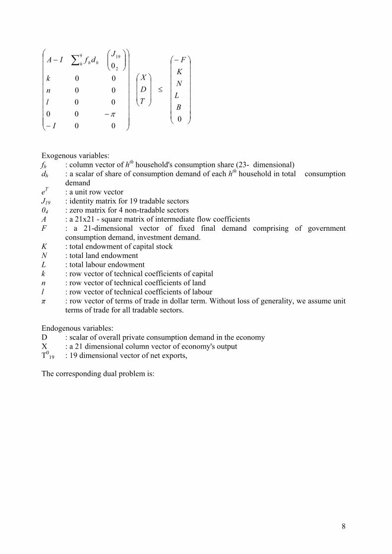
000

0000000002

199

BLNKF

TDX

I

lnk

JdfIA

h hh

π

Exogenous variables: fh : column vector of hth household's consumption share (23- dimensional) dh : a scalar of share of consumption demand of each hth household in total consumption

demand eT : a unit row vector J19 : identity matrix for 19 tradable sectors 04 : zero matrix for 4 non-tradable sectors A : a 21x21 - square matrix of intermediate flow coefficients F : a 21-dimensional vector of fixed final demand comprising of government

consumption demand, investment demand. K : total endowment of capital stock N : total land endowment L : total labour endowment k : row vector of technical coefficients of capital n : row vector of technical coefficients of land l : row vector of technical coefficients of labour π : row vector of terms of trade in dollar term. Without loss of generality, we assume unit

terms of trade for all tradable sectors. Endogenous variables: D : scalar of overall private consumption demand in the economy X : a 21 dimensional column vector of economy's output T0

19 : 19 dimensional vector of net exports, The corresponding dual problem is:

8

( )

( )

≥

=

−−

−

∂

−

∑

∑

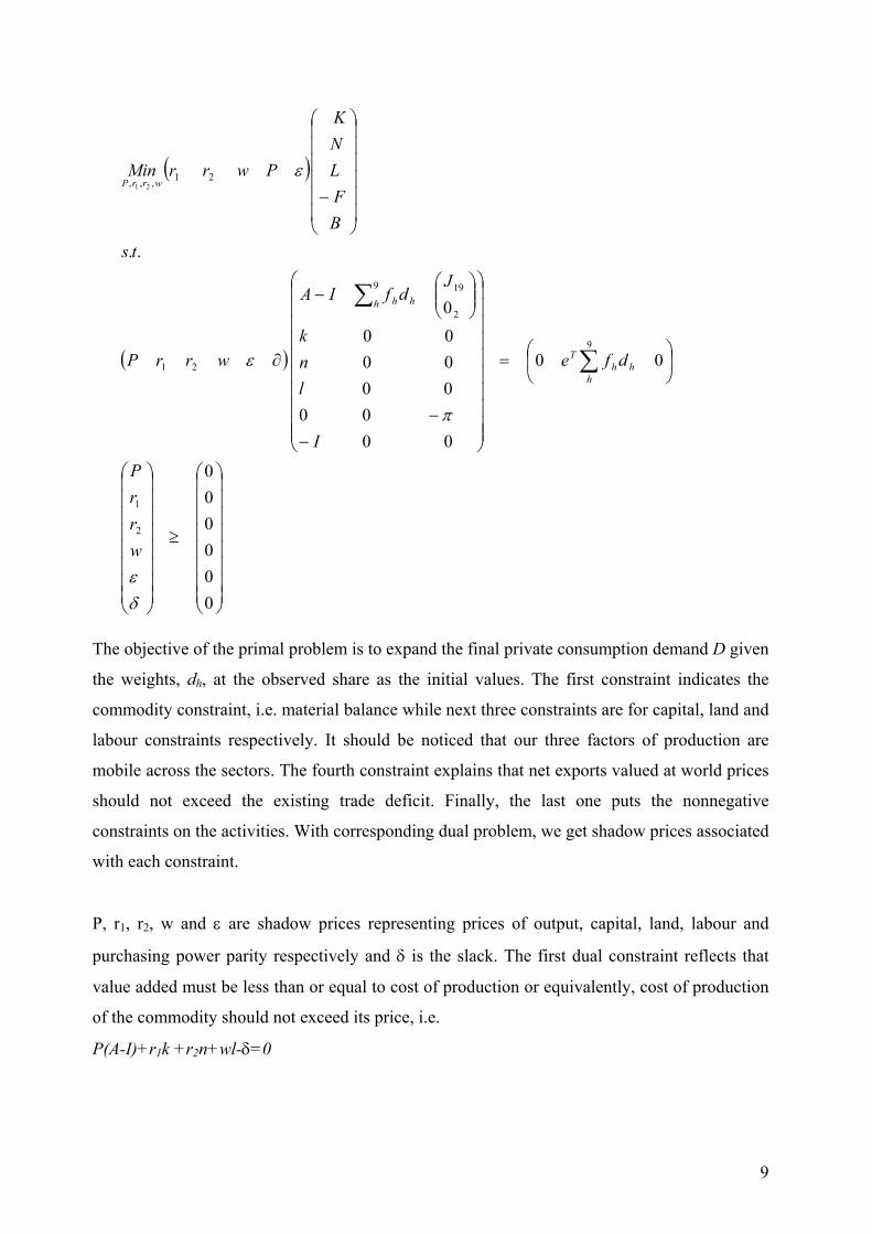
000000

00

0000

0000000

..

2

1

9

2

199

21

21,,, 21

δε

π

ε

ε

wrrP

dfe

I

lnk

JdfIA

wrrP

tsBFLNK

PwrrMin

hhh

T

h hh

wrrP

The objective of the primal problem is to expand the final private consumption demand D given

the weights, dh, at the observed share as the initial values. The first constraint indicates the

commodity constraint, i.e. material balance while next three constraints are for capital, land and

labour constraints respectively. It should be noticed that our three factors of production are

mobile across the sectors. The fourth constraint explains that net exports valued at world prices

should not exceed the existing trade deficit. Finally, the last one puts the nonnegative

constraints on the activities. With corresponding dual problem, we get shadow prices associated

with each constraint.

P, r1, r2, w and ε are shadow prices representing prices of output, capital, land, labour and

purchasing power parity respectively and δ is the slack. The first dual constraint reflects that

value added must be less than or equal to cost of production or equivalently, cost of production

of the commodity should not exceed its price, i.e.

P(A-I)+r1k +r2n+wl-δ=0

9

If the sectors are active, the non-negativity constraint is not binding, hence, associated slack

variable is zero, and price of output is equal to its cost (ten Raa, 1995). Multiplying output on

both sides, the equation becomes

P(A-I)X+r1K +r2N+wL=0

The second constraint of the dual, i.e. ∑∑ =99

h hhT

h hh dfedfP takes care of the price

normalization. The coefficient in the objective function has been selected in such a way that

only relative prices change, which is called normalization. The last constraint shows that if

trade is free, prices of the tradable commodities will be same as their opportunity costs. It

should be noted that in our case, the commodity constraint in the primal program has a non-

zero bound, i.e. due to other fixed demands in the economy, F. Using the equilibrium values

and shadow prices, we get equilibrium income level of each household group and it's

consumption level. Equality between primal and dual condition gives rise to National

Accounting balance:

r1K +r2N+wL =D∑fhdh + PF-εB

We can express this primal condition of our model in the following reduced (see Appendix II).

∑h

hhT

XDdfDeMax

,

s. t. 01919

9

][ TFDdfAXXh

hh ππ −≤−−−− ∑

[ 0]4

9

≥−−− ∑ FDdfAXXh

hh

KkX ≤ N≤nX L≤lX 0≥X The first constraint is for the 19 tradable sectors and its shadow price gives the terms trade

between tradable domestic and foreign price, ε, which is no more unit. We can derive the

domestic price by dividing foreign price, π by ε. The second constraint is for the two non-

tradable sectors. The shadow prices of this constraint give the domestic prices of non-tradable

sectors.

The next step of our methodology includes household consumption and income in a general

equilibrium framework. This is done with the help of a social accounting matrix (SAM). A

SAM captures the flows among different activities of the economy. A SAM provides a

10

framework and consistent data for economy-wide models with detailed classification of accounts

such as, industries, categories of working persons and institutional sub-sectors including various

socio-economic household groups. It can be used to provide an analysis of inter-relationship

between structural features of an economy and the distribution of income and expenditure of the

household groups. The I-O matrix, however, does not show the interrelationships between value

added and final expenditures. By extending an I-O table, to show an entire circular flow of income

at macro level, one captures the essential features of a SAM. The rows in the SAM represent the

receipts (income) of the different accounts, while the columns, their expenditure. The schematic

picture below gives a bird’s eye view about the SAM we have used for our analysis (Table 1).

Table1: A Simple Schematic SAM Production

Account Factors of Production

Households Government Capital Account

Rest of World

TOTAL

Production Account (21 sectors)

I-O Household Consumption Dfhdh

Government. Consumption

Investment Demand

Net Exports

Total Demand DeT∑fhdh

Factors of Production [labour (L), Capital (K), land (N)]

Value added (VA) kX, lX, nX

Value added

Households (9 categories)

Factor income to households (hh

l, hhk,hh

n)

Total Household Income (hh

l +hhk+hh

n) Government Account

Direct, Indirect taxes

Government Income

Capital Account

Household Savings

Government Savings

Foreign Savings

Total Savings

TOTAL

Value of Output

Value added Total Household expenditure

Total Govt Outlay

Total Investment

The second row and second column give the essence of I-O table. The crucial extension is the

inclusion of household income and expenditure (row 4 and column 4). Different household groups

owns different factor endowments and contribute to the production process as VA (column 2 x

row2) and in return get factor income according to their ownership (column 3 x row4). Though

household savings and taxes are also crucial in the general equilibrium framework, for simplicity,

we do not consider them in our analysis.

The idea is to compute the propensity to consume at the competitive prices for each household

group and in order to satisfy the general equilibrium condition, we set the ratio of new

propensity to consume to the observed one evaluated at the competitive price same for all

11

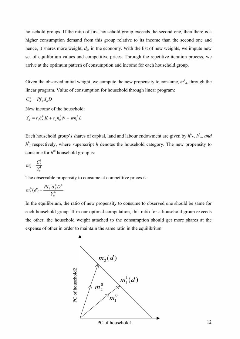
household groups. If the ratio of first household group exceeds the second one, then there is a

higher consumption demand from this group relative to its income than the second one and

hence, it shares more weight, dh, in the economy. With the list of new weights, we impute new

set of equilibrium values and competitive prices. Through the repetitive iteration process, we

arrive at the optimum pattern of consumption and income for each household group.

Given the observed initial weight, we compute the new propensity to consume, m1h, through the

linear program. Value of consumption for household through linear program:

DdPfC hhh =1

New income of the household:

LwhNhrKhrY hl

hn

hKh ++= 21

1

Each household group’s shares of capital, land and labour endowment are given by hhK, hh

n, and

hhl respectively, where superscript h denotes the household category. The new propensity to

consume for hth household group is:

1

11

h

hh Y

Cm =

The observable propensity to consume at competitive prices is:

0

000 )(

h

ho

hh Y

DdPfdm =

In the equilibrium, the ratio of new propensity to consume to observed one should be same for

each household group. If in our optimal computation, this ratio for a household group exceeds

the other, the household weight attached to the consumption should get more shares at the

expense of other in order to maintain the same ratio in the equilibrium.

01m

02m

)(12 dm

)(11 dm

PC o

f hou

seho

ld2

12PC of household1

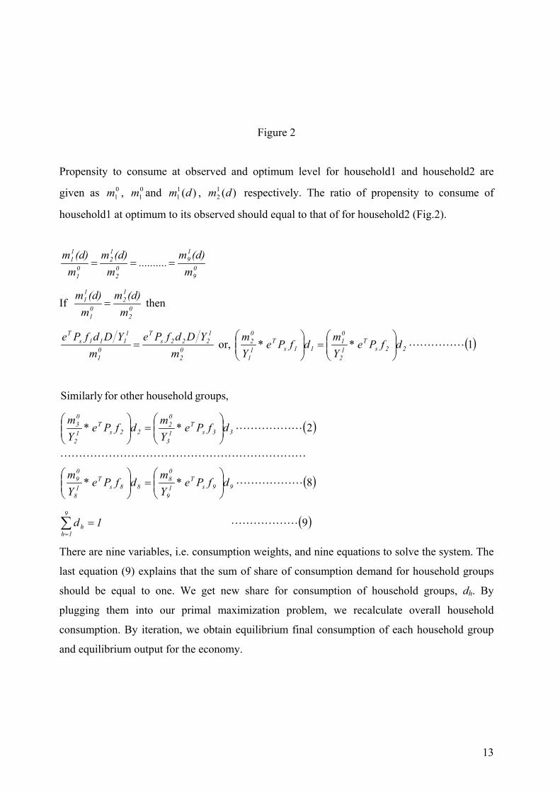
Figure 2

Propensity to consume at observed and optimum level for household1 and household2 are

given as , and , respectively. The ratio of propensity to consume of

household1 at optimum to its observed should equal to that of for household2 (Fig.2).

01m 0

1m )(11 dm )(1

2 dm

09

19

02

12

01

11

m(d)m

..........m

(d)mm

(d)m===

If 02

12

01

11

m(d)m

m(d)m

= then

02

1222s

T

01

1111s

T

mYDdfPe

mYDdfPe

= or, ( )1LLLLL22sT

12

01

11sT

11

02 dfPe*

Ym

dfPe*Ym

=

,groupshouseholdotherforSimilarly

( )2LLLLLL33sT

13

02

22sT

12

03 dfPe*

Ym

dfPe*Ym

=

( )8LLLLLL

LLLLLLLLLLLLLLLLLLLLLL

99sT

19

08

88sT

18

09 dfPe*

Ym

dfPe*Ym

=

( )9LLLLLL1d9

1hh =∑

=

There are nine variables, i.e. consumption weights, and nine equations to solve the system. The

last equation (9) explains that the sum of share of consumption demand for household groups

should be equal to one. We get new share for consumption of household groups, dh. By

plugging them into our primal maximization problem, we recalculate overall household

consumption. By iteration, we obtain equilibrium final consumption of each household group

and equilibrium output for the economy.

13

3. Benchmark Data

The Social Accounting Matrix (SAM) gives the benchmark equilibrium data set for the model.

The SAM used for the present study is based on Pradhan, Sahoo and Saluja (1999). However,

for this model, we have made some adjustment in the data (Appendix I). The intermediate flow

in the SAM is based on the commodity x commodity (C x C) matrix. This is the case where

number commodities are equal to the activity sectors and it is noticed that there is more scope

for efficient improvement then otherwise (Mattey and Raa, 1994).

Economy is classified into 21 production sectors to take care of important economic activities.

`Food-grains' has been separated from the rest of the agriculture sector for its vital role in

poverty. 'Coal and lignite', and 'crude oil and natural gas' are the two components of primary

energy. The primary energy requires higher investment in exploration and also due to high

domestic demand a substantial amount of it is imported.

The sectors in the manufacturing are divided in such a way that capital goods are separated

from consumer items like `food articles and beverages', `textiles', etc. in view of different

capital structures. For the rapid development of the economy, the `cement and other non-

metallic mineral products', which are basically inputs to the construction sector have assumed

importance. Their growth will give a fillip to the crucial housing sector as well. `Fertilisers' as a

sector has got a big role to play in influencing the agriculture. The `petroleum products' are kept

separately as these are by-products of the one of the important energy sectors, `crude oil and

natural gases'. They are also crucial energy sectors whose prices have so far been administered

and the economy is very sensitive to their price changes.

`Construction' is highly labour intensive sector and also a part of this sector gives an idea about

the physical infrastructure of the economy. `Electricity' is an important sector, having

maximum inter-linkages in the economy. `Infrastructure services' and `financial services' have

been kept as separate sectors as they have greater role to play particularly in the light of

competitive scenario leading to greater liberalisation of these sectors. Last, but not the least,

‘other services’ is an unavoidable sector in the economy which includes, public services, repair

services, services related to information technology (IT), etc. This sectors plays important role

in influencing the welfare of the economy.

14

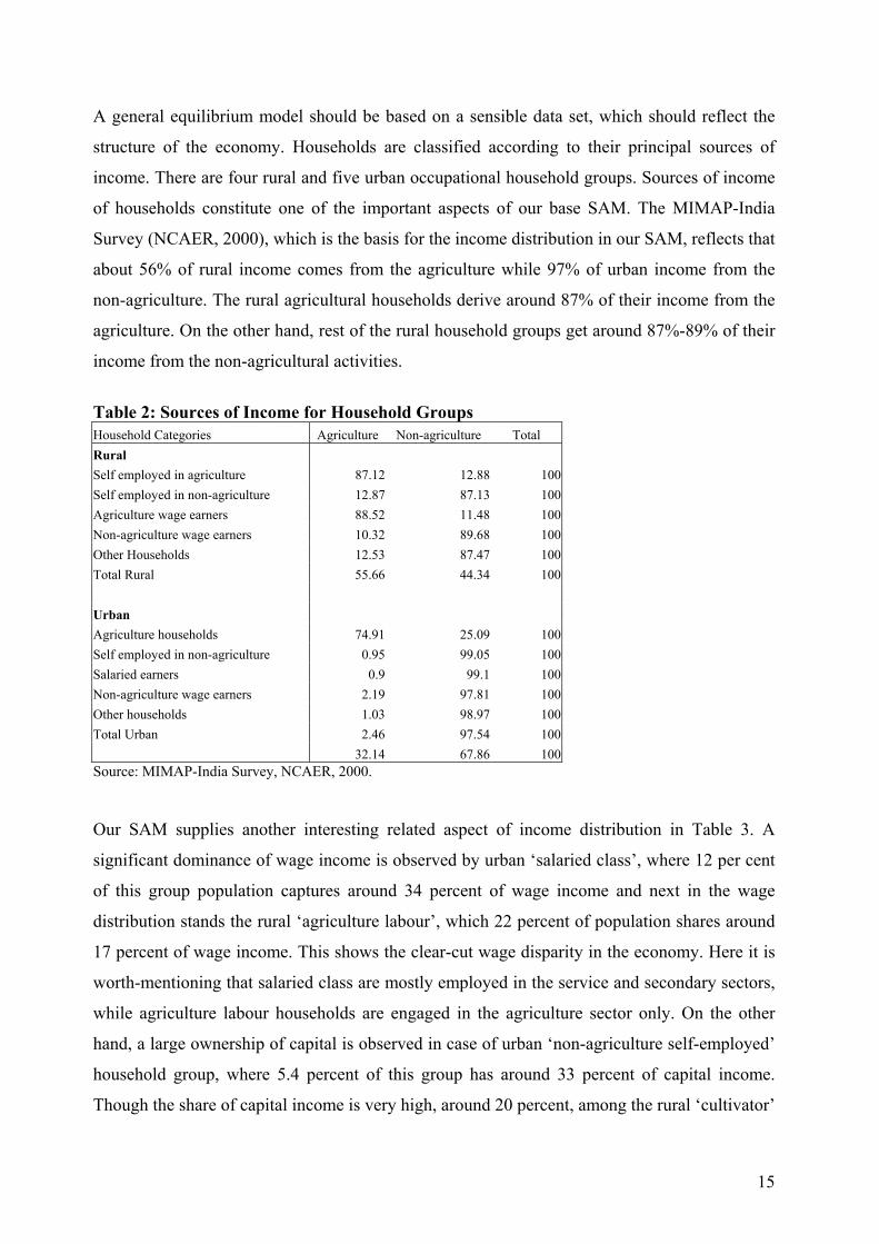
A general equilibrium model should be based on a sensible data set, which should reflect the

structure of the economy. Households are classified according to their principal sources of

income. There are four rural and five urban occupational household groups. Sources of income

of households constitute one of the important aspects of our base SAM. The MIMAP-India

Survey (NCAER, 2000), which is the basis for the income distribution in our SAM, reflects that

about 56% of rural income comes from the agriculture while 97% of urban income from the

non-agriculture. The rural agricultural households derive around 87% of their income from the

agriculture. On the other hand, rest of the rural household groups get around 87%-89% of their

income from the non-agricultural activities.

Table 2: Sources of Income for Household Groups Household Categories Agriculture Non-agriculture Total Rural Self employed in agriculture 87.12 12.88 100Self employed in non-agriculture 12.87 87.13 100Agriculture wage earners 88.52 11.48 100Non-agriculture wage earners 10.32 89.68 100Other Households 12.53 87.47 100Total Rural 55.66 44.34 100 Urban Agriculture households 74.91 25.09 100Self employed in non-agriculture 0.95 99.05 100Salaried earners 0.9 99.1 100Non-agriculture wage earners 2.19 97.81 100Other households 1.03 98.97 100Total Urban 2.46 97.54 100 32.14 67.86 100Source: MIMAP-India Survey, NCAER, 2000.

Our SAM supplies another interesting related aspect of income distribution in Table 3. A

significant dominance of wage income is observed by urban ‘salaried class’, where 12 per cent

of this group population captures around 34 percent of wage income and next in the wage

distribution stands the rural ‘agriculture labour’, which 22 percent of population shares around

17 percent of wage income. This shows the clear-cut wage disparity in the economy. Here it is

worth-mentioning that salaried class are mostly employed in the service and secondary sectors,

while agriculture labour households are engaged in the agriculture sector only. On the other

hand, a large ownership of capital is observed in case of urban ‘non-agriculture self-employed’

household group, where 5.4 percent of this group has around 33 percent of capital income.

Though the share of capital income is very high, around 20 percent, among the rural ‘cultivator’

15

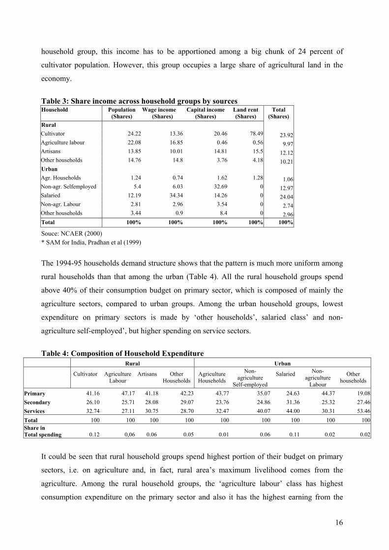
household group, this income has to be apportioned among a big chunk of 24 percent of

cultivator population. However, this group occupies a large share of agricultural land in the

economy.

Table 3: Share income across household groups by sources Household Population

(Shares) Wage income

(Shares) Capital income

(Shares) Land rent (Shares)

Total (Shares)

Rural Cultivator 24.22 13.36 20.46 78.49 23.92 Agriculture labour 22.08 16.85 0.46 0.56 9.97 Artisans 13.85 10.01 14.81 15.5 12.12 Other households 14.76 14.8 3.76 4.18 10.21 Urban Agr. Households 1.24 0.74 1.62 1.28 1.06 Non-agr. Selfemployed 5.4 6.03 32.69 0 12.97 Salaried 12.19 34.34 14.26 0 24.04 Non-agr. Labour 2.81 2.96 3.54 0 2.74 Other households 3.44 0.9 8.4 0 2.96 Total 100% 100% 100% 100% 100%

Souce: NCAER (2000) * SAM for India, Pradhan et al (1999)

The 1994-95 households demand structure shows that the pattern is much more uniform among

rural households than that among the urban (Table 4). All the rural household groups spend

above 40% of their consumption budget on primary sector, which is composed of mainly the

agriculture sectors, compared to urban groups. Among the urban household groups, lowest

expenditure on primary sectors is made by ‘other households’, salaried class’ and non-

agriculture self-employed’, but higher spending on service sectors.

Table 4: Composition of Household Expenditure

Rural Urban

Cultivator

Agriculture Labour

Artisans

Other Households

Agriculture Households

Non- agriculture

Self-employed

Salaried

Non- agriculture

Labour

Other households

Primary 41.16 47.17 41.18 42.23 43.77 35.07 24.63 44.37 19.08 Secondary 26.10 25.71 28.08 29.07 23.76 24.86 31.36 25.32 27.46 Services 32.74 27.11 30.75 28.70 32.47 40.07 44.00 30.31 53.46 Total 100 100 100 100 100 100 100 100 100Share in Total spending 0.12 0,06 0.06 0.05 0.01 0.06 0.11 0.02 0.02

It could be seen that rural household groups spend highest portion of their budget on primary

sectors, i.e. on agriculture and, in fact, rural area’s maximum livelihood comes from the

agriculture. Among the rural household groups, the ‘agriculture labour’ class has highest

consumption expenditure on the primary sector and also it has the highest earning from the

16

agriculture sector, 89 percent (Table 2). In urban area, except for the ‘agriculture households’

and ‘non-agriculture labour, whose share in total spending in the economy is very low, 0.01 and

0.02 respectively, expenditure on service sector constitutes highest in their consumption baskets

while they earn their income maximum from non-agriculture sector. This rural and urban

dichotomy may play an interesting role in influencing economic activities of the country. It is

noted that the spending on secondary sector, comprising manufacturing sectors and ‘electricity’

in it, does not show much variability except for the case of urban ‘salaried class’ who allocates

relatively more of its budget share than other household groups.

3.1. Data for the Model The social accounting matrix for India by Prdhan et al. (1999) provides the base data for our

model. The original SAM has 60 production sectors. For our purpose, we aggregated them to

21 sectors. As already discussed above, besides giving data on intermediate flows and value

added of different factors the SAM provides information on the total household consumption,

consumption share of household groups in the total demand and consumption vectors of

commodities. It also gives us information on the endowment of different factors by various

household groups. Major problem is encountered to set the benchmark price for labour, capital

and land, hence, the factor-output ratios for the primal problem.

Given the diverse activities in the Indian economy, wages are expected to vary across different

sectors. Annual Survey of Industry (ASI) (Government of India, 1994-95) gives information on

number of employees engaged in different registered manufacturing industries and their total

emoluments. We compute the average wage rate for each industry. However, because of the

difficulty in procuring information on unregistered industries, we assume the same wage rates

for all India industries. By applying these wage rates on SAM labour value added, we estimated

number of employees, i.e. labour supply for manufacturing industries. However, ASI does not

give information on agriculture sectors, mining and quarrying, construction and service sectors.

Using the information on number of main and marginal workers engaged in these activities

given by Census of India (1991), we compute the benchmark wage rate for these sectors. Total

labour force is not fully employed in the model. Unemployment rate of 6 percent is applied to

the labour constraint equation in the model5.

5 Unemployment rate is the ratio of unemployed to the total labour force based on daily status. The source is “National Sample Survey Organisation. Report no.409. Employment and Unemployment in India, 1993-94: NSS Fiftieth Round. July 1993-June 1994. New Delhi.1997”

17

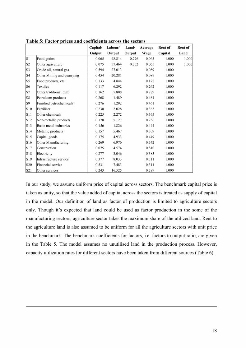
Table 5: Factor prices and coefficients across the sectors Capital/ Labour/ Land/ Average Rent of Rent of Output Output Output Wage Capital Land S1 Food grains 0.065 48.814 0.276 0.065 1.000 1.000 S2 Other agriculture 0.075 57.464 0.302 0.065 1.000 1.000 S3 Crude oil, natural gas 0.594 27.013 0.089 1.000 S4 Other Mining and quarrying 0.454 20.281 0.089 1.000 S5 Food products, etc. 0.133 4.844 0.172 1.000 S6 Textiles 0.117 6.292 0.262 1.000 S7 Other traditional mnf. 0.162 5.808 0.289 1.000 S8 Petroleum products 0.268 1.489 0.461 1.000 S9 Finished petrochemicals 0.276 1.292 0.461 1.000 S10 Fertiliser 0.230 2.028 0.365 1.000 S11 Other chemicals 0.225 2.272 0.365 1.000 S12 Non-metallic products 0.170 5.127 0.236 1.000 S13 Basic metal industries 0.156 1.826 0.444 1.000 S14 Metallic products 0.157 5.467 0.309 1.000 S15 Capital goods 0.175 4.933 0.449 1.000 S16 Other Manufacturing 0.269 6.976 0.342 1.000 S17 Construction 0.075 4.574 0.810 1.000 S18 Electricity 0.277 3.046 0.383 1.000 S19 Infrastructure service 0.377 8.033 0.311 1.000 S20 Financial service 0.531 7.483 0.311 1.000 S21 Other services 0.243 16.525 0.289 1.000

In our study, we assume uniform price of capital across sectors. The benchmark capital price is

taken as unity, so that the value added of capital across the sectors is treated as supply of capital

in the model. Our definition of land as factor of production is limited to agriculture sectors

only. Though it’s expected that land could be used as factor production in the some of the

manufacturing sectors, agriculture sector takes the maximum share of the utilized land. Rent to

the agriculture land is also assumed to be uniform for all the agriculture sectors with unit price

in the benchmark. The benchmark coefficients for factors, i.e. factors to output ratio, are given

in the Table 5. The model assumes no unutilised land in the production process. However,

capacity utilization rates for different sectors have been taken from different sources (Table 6).

18

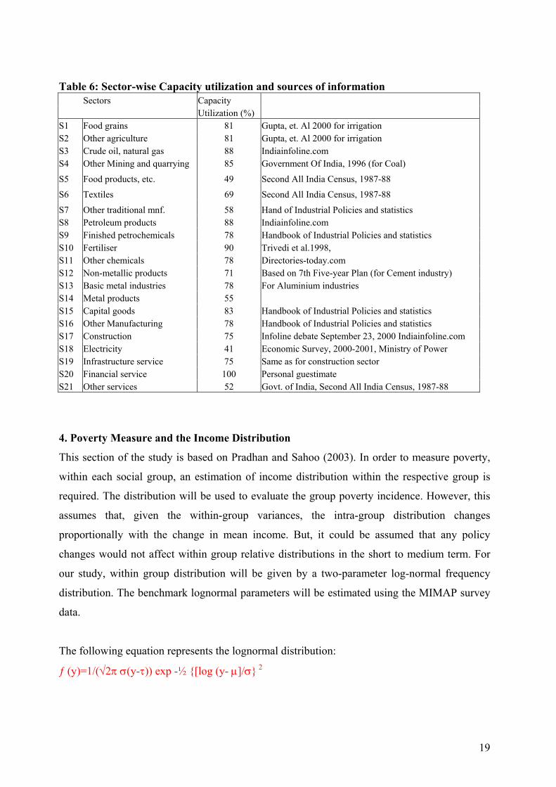
Table 6: Sector-wise Capacity utilization and sources of information Sectors Capacity Utilization (%) S1 Food grains 81 Gupta, et. Al 2000 for irrigation S2 Other agriculture 81 Gupta, et. Al 2000 for irrigation S3 Crude oil, natural gas 88 Indiainfoline.com S4 Other Mining and quarrying 85 Government Of India, 1996 (for Coal)

S5 Food products, etc. 49 Second All India Census, 1987-88

S6 Textiles 69 Second All India Census, 1987-88

S7 Other traditional mnf. 58 Hand of Industrial Policies and statistics S8 Petroleum products 88 Indiainfoline.com S9 Finished petrochemicals 78 Handbook of Industrial Policies and statistics S10 Fertiliser 90 Trivedi et al.1998, S11 Other chemicals 78 Directories-today.com S12 Non-metallic products 71 Based on 7th Five-year Plan (for Cement industry) S13 Basic metal industries 78 For Aluminium industries S14 Metal products 55 S15 Capital goods 83 Handbook of Industrial Policies and statistics S16 Other Manufacturing 78 Handbook of Industrial Policies and statistics S17 Construction 75 Infoline debate September 23, 2000 Indiainfoline.com S18 Electricity 41 Economic Survey, 2000-2001, Ministry of Power S19 Infrastructure service 75 Same as for construction sector S20 Financial service 100 Personal guestimate S21 Other services 52 Govt. of India, Second All India Census, 1987-88

4. Poverty Measure and the Income Distribution

This section of the study is based on Pradhan and Sahoo (2003). In order to measure poverty,

within each social group, an estimation of income distribution within the respective group is

required. The distribution will be used to evaluate the group poverty incidence. However, this

assumes that, given the within-group variances, the intra-group distribution changes

proportionally with the change in mean income. But, it could be assumed that any policy

changes would not affect within group relative distributions in the short to medium term. For

our study, within group distribution will be given by a two-parameter log-normal frequency

distribution. The benchmark lognormal parameters will be estimated using the MIMAP survey

data.

The following equation represents the lognormal distribution:

ƒ (y)=1/(√2π σ(y-τ)) exp -½ {[log (y- µ]/σ} 2

19

where µ, and σ are mean income and standard deviation of log-normal distribution,

respectively. For the purpose of our poverty analysis, we would use only head-count ratio as

one of the three special cases of FGT poverty measure (Foster, Greer and Thorbecke, 1984).

The FGT measure is especially suitable to estimate group-wise poverty. The FGT measure is

defined by α

iα Z

Y-Zn1P ∑

= ,

where Z is the poverty line, n is the number of persons in a particular household group (i.e.

occupational class), and Yi is the income of the ith household group. The α can be viewed as a

measure of poverty aversion. The three special cases of FGT measure where α takes value 0, 1

and 2 are the most commonly used. When α=0, P0 becomes the 'head-count ratio measure', when

α=1, P1 is the 'poverty-gap measure' and α=2, P2 becomes distributionally sensitive measure'.

The higher degree of 'poverty aversion', i.e. α=2, indicates that the poorest person should get

relatively more weight in the poverty measure. In this paper, we have used only head count ratio of

poverty measure for our analysis. However, it is not difficult to use the other measures. In the plain

language the poverty head-count ratio of particular household group is the ratio of number

households living below the poverty line to total population in the group.

When income distribution is given in the form of group data, the poverty measure requires a

continuous distribution. We now intend to express the poverty measure in terms of lognormal

distribution. The above-mentioned Pα measure would no longer be based on the discrete

information. It is expressed in continuous distribution.

dy),I(Z

Y-ZPα

σµα ∫

=

z

0,

where I(µ,σ) is the income distribution of the household group. The distribution varies from 0

to z. After transformation of the right hand side of the equation, the 'head-count ratio' becomes

==

σµσµ -log(z)GIP 00 ),( .

The right hand side of the expression is the standard normal distribution. Likewise one can

compute the transformed expressions for P1 and P2.

20

Poverty line Z would be endogenised in our model through changes in the relative commodity

prices. The change in mean income of household group will come from optimum solution of

our model6.

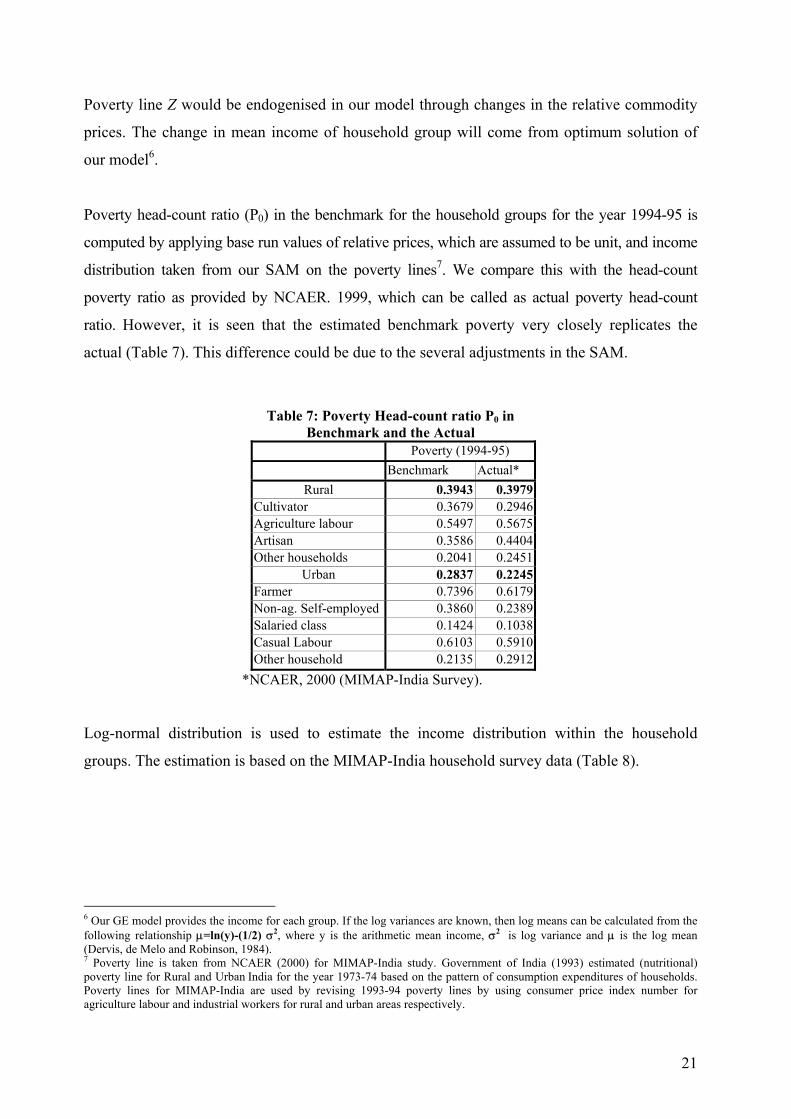
Poverty head-count ratio (P0) in the benchmark for the household groups for the year 1994-95 is

computed by applying base run values of relative prices, which are assumed to be unit, and income

distribution taken from our SAM on the poverty lines7. We compare this with the head-count

poverty ratio as provided by NCAER. 1999, which can be called as actual poverty head-count

ratio. However, it is seen that the estimated benchmark poverty very closely replicates the

actual (Table 7). This difference could be due to the several adjustments in the SAM.

Table 7: Poverty Head-count ratio P0 in Benchmark and the Actual

Poverty (1994-95) Benchmark Actual*

Rural 0.3943 0.3979Cultivator 0.3679 0.2946Agriculture labour 0.5497 0.5675Artisan 0.3586 0.4404Other households 0.2041 0.2451

Urban 0.2837 0.2245Farmer 0.7396 0.6179Non-ag. Self-employed 0.3860 0.2389Salaried class 0.1424 0.1038Casual Labour 0.6103 0.5910Other household 0.2135 0.2912

*NCAER, 2000 (MIMAP-India Survey).

Log-normal distribution is used to estimate the income distribution within the household

groups. The estimation is based on the MIMAP-India household survey data (Table 8).

6 Our GE model provides the income for each group. If the log variances are known, then log means can be calculated from the following relationship µ=ln(y)-(1/2) σ2, where y is the arithmetic mean income, σ2 is log variance and µ is the log mean (Dervis, de Melo and Robinson, 1984). 7 Poverty line is taken from NCAER (2000) for MIMAP-India study. Government of India (1993) estimated (nutritional)

poverty line for Rural and Urban India for the year 1973-74 based on the pattern of consumption expenditures of households. Poverty lines for MIMAP-India are used by revising 1993-94 poverty lines by using consumer price index number for agriculture labour and industrial workers for rural and urban areas respectively.

21

Table 8: Parameters of log-normal distribution Log-

mean Standard deviation

Rural Cultivator 5.85 0.76 Agriculture labour 5.33 0.60 Artisan 5.55 0.79 Other household 5.93 0.72 Urban Farmer 5.41 1.05 Non-ag. Self-employed 6.36 0.89 Salaried Class 6.68 0.76 Casual Labour 5.54 0.82 Other Household 6.47 1.35

For our measure of inequality, we use standard Gini coefficient, which is often based on and

derived from the Lorenz curve. We derive our Gini coefficients from Lorenze curve. Lorenze

curve is a plot of cumulative fraction of population, starting from the lowest income, on the x-

axis against cumulative fraction of population of the household groups on y-axis. If the

resources were equally distributed, the Lorenze curve would be 45-degree line. The Gini is the

area between the curve and 45-degree line as fraction of 0.5, which is the total area under 45-

degree line (Fig.3).

5. Results and Implications

The main concern of this paper is to see the efficiency gain due to competitiveness in the

economy resulted from possible economic reform process, which may result in the change in

the income distribution and poverty among the household groups. If the hypothetical Indian

economy under analysis is operating below the optimal level, then the expansion of domestic

private final demand will reach the frontier by doing away with the slacks in the factor use and

reallocation of resources. In the free trade environment, endogenizing the trade with net exports

constraint will take care of the terms of trade effect, which in a way captures the gain in the

technical efficiency.

Since 1991, the beginning of the era of full pace economic reform, there has been a great deal

of debate in India about the possible impact of these policies on the poor. If one looks at the

head count poverty ratio for rural and urban India since 1983, it is seen that rural poverty ratio

has been always higher than that for urban (Table 9). The decline in the poverty ratio started in

the late eighties itself. This is not, however, an unusual phenomenon, given the size of rural

population. In the pre-reform period, until 1990, both the rural and the urban poverty have

declined. It could be mentioned that there was some well-thought initiation of reform process,

22

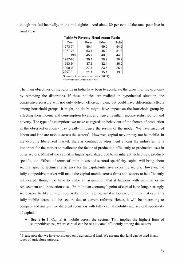
though not full heartedly, in the mid-eighties. And about 80 per cent of the total poor live in

rural areas.

Table 9: Poverty Head-count Ratio Year Rural Urban Total

1973-74 56.4 49.0 54.91977-78 53.1 45.2 51.3

1983 45.7 40.8 44.51987-88 39.1 38.2 38.91993-94 37.3 32.4 36.01999-00 27.1 23.6 26.12007 * 21.1 15.1 19.3

The main objectives of the r

by removing the distortio

competitive pressure will n

among household groups. I

affecting their income and

poverty. The type of assump

in the observed economy m

labour and land are mobile

the evolving liberalized m

important for the market to

other sectors. Most of the c

specific, etc. Effects of term

sectoral specific technical e

fully competitive market wi

reallocated, though we ha

replacement and transaction

sector-specific like during i

fully mobile across all the

compare and analyse two di

of capital.

• Scenario 1. Capitalcompetitiveness, wh

8 Please note that we have contypes of agriculture purpose.

Source: Government of India (2003)*Poverty projection for 2007

eforms in India have been to accelerate the growth of the economy

ns. If these policies are realized in hypothetical situation, the

ot only deliver efficiency gain, but could have differential effects

t might, no doubt might, have impact on the household group by

consumption levels, and hence, resultant income redistribution and

tions we make as regards to behaviour of the factors of production

ay greatly influence the results of the model. We have assumed

across the sectors8. However, capital may or may not be mobile. In

arket, there is continuous adjustment among the industries. It is

reallocate the factor of production efficiently to productive uses in

apital is highly specialized due to its inherent technology, product-

s of trade in case of sectoral specificity capital will bring about

fficiency for the capital-intensive exporting sectors. However, the

ll make the capital mobile across firms and sectors to be efficiently

ve to make an assumption that it happens with minimal or no

costs. From Indian economy’s point of capital is no longer strongly

mport-substitution regime, yet it is too early to think that capital is

sectors due to current reforms. Hence, it will be interesting to

fferent scenarios with fully capital mobility and sectoral specificity

is mobile across the sectors. This implies the highest form of ere capital can be re-allocated efficiently among the sectors.

23

sidered only agricultural land. We assume that land can be used in any

• Scenario 2. Capital is immobile and sector specific. In this case, we may lose the

degree of efficiency due to constraint on capital re-allocation. If the economy is operating under a competitive spirit with free trade and all the factors of

productions are mobile, as in Scen.1, the expansion factor of the frontier at the optimal solution

is 1.64 as compared to one in the benchmark. The total efficiency of the economy is 1/1.46 =

0.68, indicating that economy would achieve its potential 68 percent more than the observed

performance. Despite the productivity growth, the inequality as represented by Gini coefficient

has significantly increased to 0.3675 at the optimum from 0.2739 at the actual level. Poverty as

measure of head-count ratio (P0), as defined in the Section4 declines sharply urban households,

while it has deteriorated for rural households (Table 11). This is because of the adverse income

distribution of rural households against the urban households. Except for the rural artisans,

income ratio of optimum to observed decline for all other rural household groups.

Our observed Indian economy has around 6 percent of unemployment rate in the labour force

and sector specific unutilised capital. When the economy is allowed to be competitive to

operate at the optimum, the mobile factors are reallocated themselves to the sectors where

demand for demand for respective factor is more. Shadow prices of labour and capital are

picked up by the two factor constrains. The factor mobility gives rise to one competitive factor

price for each factor. In this scenario, we observe that demand for capital has been higher than

that of labour. The removal of slack in the capital constraint results in more efficient use of

unutilised capital. Land is seen to be non-binding at the optimum, yielding a zero shadow price.

This hints at the fact that there is no scope to improve the efficiency of agricultural land use.

Factor prices of capital and labour have increased at the optimum. The ratios of optimum factor

prices to observed for capital and labour are 2.24 and 0.73 respectively (Table 10). Lagrange

multipliers to the material balance and balance of constraints in the primal give the commodity

prices and exchange rate respectively under competitive conditions, which are determined in

the dual constraint. As we have already discussed in the model that cost and revenue of the

sector must equate in the dual program. When the factors are binding, rise in the factor prices

must either raise in the optimal commodity price or output. In our case, prices of tradable

commodities are the same as the optimal exchange rate as the benchmark terms of trade is

assumed to be one. It should also be noted that if there is an increase in price of non-tradable

commodity, it must be driven by at the cost of price of commodities produced by the tradable

sectors.

24

At this point it’s important to mention that our kind of linear programming models give rise to

specialisation in the production sectors. Theoretically, we have three factor constraints and two

constraints for non-tradable sectors and hence, we expect five active sectors in the economy.

However, land is found to be non-binding, resulting in four active sectors in Indian economy,

viz. ‘food grains’ (S15), ‘construction’ (S17), ‘electricity’ (S18) and ‘other services’ (S21), of

which construction and electricity are non-tradable sectors (Table 10). The ‘other service

sector’, which includes information technology, (IT) shows a significant performance in the

productivity at the optimum level with 7.72 times better than the actual. Free movement of

factors, particularly capital, and free trade is expected to give boost to the service sector in the

economy, which has already started realizing in India. The ‘construction’ comes next in the

increase in the output followed by ‘food grains’. Output declines for ‘electricity’ sector, while

the price of this domestic non-tradable sector increases by factor 1.33. Productivity growth in

other three active sectors results in decrease in their prices. Ever since the reform process

started, globalizing of the agriculture sector has been a moot issue. In this perspective, our

result that the ‘food grains’ as an important sub-sector of agriculture becoming active with

increasing growth would support the globalizers. However, the most important question is

which household group benefits from this.

As factor price of capital increases more than that of the labour, we expect that household

groups owning more capital would gain in this allocation process. Table 4 shows that among

rural household groups, the ‘cultivator’ households have highest capital as well as land

ownership. Their consumption weight has declined due to zero land prices at the optimum.

However, only ‘artisan’ household group gains in weight due to capital reward. The worst

affected household group in the economy is the rural ‘agricultural labour’, which has very low

share of capital and large labour endowment. On the other hand, among urban household

groups, ‘salaried class’ has maximum contribution of labour, which contributes to its decline in

consumption share and maximum gain incurs to the ‘non-agricultural self-employed’ household

group. The wide income disparity between rural and urban household groups has given rise to

increase in the Gini coefficient, the measure of inequality. Within rural household groups,

income distribution is strongly biased towards the ‘artisan’ group and against the ‘agricultural

labour’.

25

Change in poverty ratio is reflected by the inter-play of change in price and income. Adverse

income effect among most of the rural household groups dominantly explains the increase in

rural poverty ratio. While only the ‘artisan’ household group shows a significant decline in

poverty, the ‘ agricultural labour’ suffers heavily from increase in poverty ratio. Poverty ratio

increases by around 17 percent for rural ‘agriculture labour’ household group. With already

high existing poverty ratio for this group, i.e. 0.55, the significant rise in poverty will certainly

have disastrous effect on them. On the other hand, there is a sharp decline in the urban poverty.

However, decline in poverty ratio is the least for the highly labour-endowed salaried class,

because of its lower increase in income.

In the Scen.2, we consider capital is sector-specific and it is difficult to reallocate them among

sectors. We take the same rate of capacity utilization as Scen.1. The basic differences of this

scenario from the earlier one are that in present scenario, economy experiences less expansion

vector due to lack of re-allocation of capital in the observed economy and unlike earlier case,

there are not any more few specialized sector, rather all sectors are active. The expansion factor

is now 1.42 and total efficiency is 1/1.42 = 0.70. There is also an increase in inequality in the

economy. But it is interesting to see that the increase in inequality has been less than the earlier

scenario. Gini coefficient is now 0.3448. This less degree of inequality vis-à-vis the previous

scenario could be assigned to the marginal improvement in the income distribution among the

rural household groups. On the other hand poverty head-count ratio (P0) declines for overall

rural and urban households (Table 11). The decline is quite significant for the urban household

as against the marginal decline for the overall rural households. Like the Scenario 1, this case

also change in poverty ratio seems to be dominated by the income effect of household groups.

Each production activity has to produce within its fixed amount of capital along with mobile

labour and land. There may be more extensive use of capital at the optimum, as the competition

would lead to exploitation of unutilised capital till its full utilization. Rent to capital is

determined by interplay of demand and supply of each industry; therefore, we get different

optimum rent for different industries. Fixed supply of capital as against the flexible labour

drives the capital price more than the wage for most of the sector. In fact, the competitive wage

has declined with respect to benchmark. On the other hand, capital rent has declined

significantly for most labour-intensive primary sectors: ‘food grains, ‘crude oil and natural gas’

and ‘other mining and quarrying’ (Table 10). Even we notice non-binding in the capital

constraint for ‘other agriculture’ sector (S2). We also observe two more non-bindings in the

26

capital constraints of two non-tradable sectors, viz. ‘construction’ (S17) and ‘electricity’ (S18).

Like the earlier scenario, land constraint is found to be non-binding yielding zero shadow price.

We see that sectors pay higher rents to capital because of their increased use of industry-

specific capital. At the same time, sectors with low initial utilization rates, experience growth in

output. Sector like ‘food and food products’ (S5) has shown significant increase in output with

respect to observed level, 2.04, followed by ‘other services’ (S21), 1.92, and ‘metallic products’

(S14), 1.81. It should be kept in mind that these sectors are also open to free trade. Though the

‘electricity’ sector (S18), which is not tradable, has the lowest initial capacity utilization rate, it

shows relatively much less increase in output. This could draw upon the fact that when capital

is sector-specific, efficiency due to re-orientation of trade plays a significant role in sectoral

growth. The relative prices of commodities produced under free trade go up marginally vis-à-

vis lower prices of non-tradable commodities. Increase in domestic production has resulted in

the marginal increase in exchange rate.

Decline in competitive wage, i.e. with ratio of optimum to observed wage being 0.92, combined

with the variation of rent to capital would influence the change in income of household groups

at the optimum solution. The slump in wage and capital rent in agricultural sectors has adverse

effect on income of rural ‘agriculture labour’ and ‘cultivator’ class respectively. Among the

rural household groups, ‘artisan’ household group gains in income distribution and

consumption weight. On the other hand, urban household groups have shown relatively better

performance in income and hence, consumption weights except for the ‘salaried class’, who has

got highest endowment of labour. Income inequality has also increased, but less than the earlier

scenario. The reason for less increase in inequality as compared to earlier scenario is that rural

household groups, especially the lowest income groups who are responsible for the rural

welfare distribution, viz. the ‘agriculture labour’ and other household’, performed better in

income ratio and consumption weight distribution than in the previous scenario. This is mainly

because of lower decline in wage than in the previous case of capital mobility across sectors.

Income effect again plays a significant role in influencing household poverty head count ratio.

Rural household groups, engaged in the agriculture sectors, viz. ‘cultivator’ and ‘agricultural

labour’, have experienced increase in poverty ratio. However, the increase in poverty for

agricultural labour is much significantly less than that of in case of mobility mobile capital due

to improvement in their income level as compared to earlier case. Urban household groups

enjoy the decline in poverty ratio, with marginally better than the earlier scenario.

27

6. Conclusion

This paper discusses the efficiency gain of Indian economy due to efficient re-allocation

internal resources as well as re-orientation of free trade. However, we do not direct our analysis

towards the degree of contribution of various efficiencies. We go further to look into the impact

of the efficiency gain on the income distribution of household groups and their poverty. Income

of households changes with the new competitive factor prices. Given the fixed savings rate for

individual household group, there is scope for readjustment of consumption weights of

household groups until ratio of new optimal propensity consume to observed one equals for all

the household groups.

As the economic theory suggest, welfare maximization may not result in positive income

distribution in the first best case. Indian economy, so far, has been operating below the efficient

resource allocation and lack of competition. Its pursuit for welfare maximization under

competitive spirit has no doubt resulted in efficiency gain, but at the cost of adverse income

distribution. Rural household groups suffer more than the urban ones. Poverty head-count ratio

as measure of poverty of household groups is determined by change in price and income

distribution. The study shows that the income effect dominates the in influencing poverty ratio

at the optimum allocation. Income distribution worsens in both the cases of capital mobility and

sector specificity. This could also be traced in the variation in the poverty ratio across the

household groups. Urban household groups, in general gain in welfare distribution with

significant decline in poverty headcount ratio as against the rural household groups. The only

rural household group, who experiences significant decline in poverty, is the ‘artisan’. But, the

worst sufferers in all accounts are rural ‘agricultural labour’ due to resultant poor wage rate at

the optimum allocation. Among the urban household groups, relative gain for ‘salaried class’ is

very low. Though degree of inequality and poverty varies with our assumption pertaining to

factor capital mobility across the sectors, the intensity of variation is not strikingly different

from each other. Nevertheless, capital mobility results in higher productivity growth due to

efficient utilization of resources with resultant higher degree of inequality. On the other hand,

poverty salutation is marginally better in case sectoral specificity of capital.

The study is, no doubt, not without having some shortcomings. Like many other applied

models, our model is great constrained by proper data availability, particularly for the sector-

28

wise capacity utilization rate of capital. We have simplified our model by not incorporating the

taxes in the material balance constraint as well as in the objective function. We allowed for free

trade without any tariff or non-tariff barriers, which is not very realistic in Indian situation. Our

iteration for readjustment of our consumption weights is limited by the fixed saving rate of

household group and not allowing for any income transfer among inter-household groups. We

take very simplified measure income distribution, Gini, which should have considered large

number of household groups. Besides, it does not take into account the intra-household group

distribution. Despite all these admitted shortcomings, the study gives a basis to explore more

interesting possibilities to link between productivity-efficiency gain and household conditions.

Given the vastness of Indian economy and heterogeneous household characteristics, general

equilibrium analysis has, no doubt, been appropriate to capture the impacts on the household

groups through inter-linkages in the economy.

29

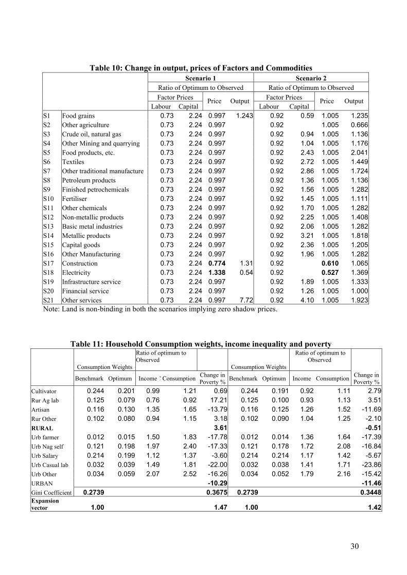
Table 10: Change in output, prices of Factors and Commodities Scenario 1 Scenario 2 Ratio of Optimum to Observed Ratio of Optimum to Observed

Factor Prices Factor Prices Labour Capital

Price Output Labour Capital

Price Output

S1 Food grains 0.73 2.24 0.997 1.243 0.92 0.59 1.005 1.235S2 Other agriculture 0.73 2.24 0.997 0.92 1.005 0.666S3 Crude oil, natural gas 0.73 2.24 0.997 0.92 0.94 1.005 1.136S4 Other Mining and quarrying 0.73 2.24 0.997 0.92 1.04 1.005 1.176S5 Food products, etc. 0.73 2.24 0.997 0.92 2.43 1.005 2.041S6 Textiles 0.73 2.24 0.997 0.92 2.72 1.005 1.449S7 Other traditional manufacture 0.73 2.24 0.997 0.92 2.86 1.005 1.724S8 Petroleum products 0.73 2.24 0.997 0.92 1.36 1.005 1.136S9 Finished petrochemicals 0.73 2.24 0.997 0.92 1.56 1.005 1.282S10 Fertiliser 0.73 2.24 0.997 0.92 1.45 1.005 1.111S11 Other chemicals 0.73 2.24 0.997 0.92 1.70 1.005 1.282S12 Non-metallic products 0.73 2.24 0.997 0.92 2.25 1.005 1.408S13 Basic metal industries 0.73 2.24 0.997 0.92 2.06 1.005 1.282S14 Metallic products 0.73 2.24 0.997 0.92 3.21 1.005 1.818S15 Capital goods 0.73 2.24 0.997 0.92 2.36 1.005 1.205S16 Other Manufacturing 0.73 2.24 0.997 0.92 1.96 1.005 1.282S17 Construction 0.73 2.24 0.774 1.31 0.92 0.610 1.065S18 Electricity 0.73 2.24 1.338 0.54 0.92 0.527 1.369S19 Infrastructure service 0.73 2.24 0.997 0.92 1.89 1.005 1.333S20 Financial service 0.73 2.24 0.997 0.92 1.26 1.005 1.000S21 Other services 0.73 2.24 0.997 7.72 0.92 4.10 1.005 1.923Note: Land is non-binding in both the scenarios implying zero shadow prices.

Table 11: Household Consumption weights, income inequality and poverty

Consumption Weights

Ratio of optimum to Observed Consumption Weights

Ratio of optimum to Observed

Benchmark Optimum Income C Consumption Change in Poverty % Benchmark Optimum Income Consumption Change in

Poverty %Cultivator 0.244 0.201 0.99 1.21 0.69 0.244 0.191 0.92 1.11 2.79Rur Ag lab 0.125 0.079 0.76 0.92 17.21 0.125 0.100 0.93 1.13 3.51Artisan 0.116 0.130 1.35 1.65 -13.79 0.116 0.125 1.26 1.52 -11.69Rur Other 0.102 0.080 0.94 1.15 3.18 0.102 0.090 1.04 1.25 -2.10RURAL 3.61 -0.51Urb farmer 0.012 0.015 1.50 1.83 -17.78 0.012 0.014 1.36 1.64 -17.39Urb Nag self 0.121 0.198 1.97 2.40 -17.33 0.121 0.178 1.72 2.08 -16.84Urb Salary 0.214 0.199 1.12 1.37 -3.60 0.214 0.214 1.17 1.42 -5.67Urb Casual lab 0.032 0.039 1.49 1.81 -22.00 0.032 0.038 1.41 1.71 -23.86Urb Other 0.034 0.059 2.07 2.52 -16.26 0.034 0.052 1.79 2.16 -15.42URBAN -10.29 -11.46Gini Coefficient 0.2739 0.3675 0.2739 0.3448Expansion vector 1.00 1.47 1.00 1.42

30

Chart 1: Benchmark Consumption Weights of

Household Groups

25%

13%

12%10%1%

12%

21%

3% 3% Cultivator

Rur Ag lab

Artisan

Rur Other

Urb farmer

Urb Nag self

Urb Salary

Urb Casual lab

Urb Other

Chart 2 Consumption Weights of Household Groups in Scenario 1

20%

8%

13%

8%1%20%

20%

4% 6% CultivatorRur Ag labArtisanRur OtherUrb farmerUrb Nag selfUrb SalaryUrb Casual labUrb Other

Chart 3: Consumption Weights of Household groups in Scenario 2

19%

10%

12%

9%1%18%

22%

4% 5%Cultivator

Rur Ag lab

Artisan

Rur Other

Urb farmer

Urb Nag self

Urb Salary

Urb Casual lab

Urb Other

31

References

Adelman, I., and S. Robinson (1978), Income Distribution Policy in developing Countries: A case study of

Korea, Stanford, CA: Stanford University Press. Adelman, I., and S. Robinson (1988), "Macro economic Adjustment and Income Distribution- Alternative

Models Applied to Two Economies", Journal of Development Economics, Vol. 29, 23-44. Annual Survey of Industries, Central Statistical Organisation (Various Issues), Department of Statistics,

Ministry of Planning and Programme Implementation, Govt. of India. Armington, P.S. (1969), "A Theory of Demand for Products Distinguished by Place of Production",

International Monetary Fund Staff Papers, Vol. 16, 159-76. Armington, P.S. (1969), " The Geographic Pattern of Trade and the Effects of Price Changes", International

Monetary Fund Staff Papers 16, 176-199. Armington, P.S. (1970), "Adjustment of trade Balances: Some Experiments with a Model of Trade

Among Major Countries", International Monetary Fund Staff Papers, Vol. 17, 488-523. Bajpai, N. and J. D. Sachs (1997), “India’s Economic Reforms: Some Lessons from East Asia”, Journal

of International Trade and Economic Development, Vol. 6(2), 135-164. Bhagwati, J. and T.N. Srinivasan (1993), “India’s Economic Reform”, Paper prepared for the Ministry

of Finance, Government of India, Delhi. Bhagwati, J. (1994), “Free Trade: Old and New Challenges”, Economic Journal, Vol.104 (423), 231-

246. Cogneau, D. and C. Guenard (2002), Can “Relationship be found between Inequality and Growth”,

Documents de travail DIAL, in Dial- Paris Development Seminar, Paris. Debreu, G. (1959), Theory of value, Yale University Press, New Haven, CT. Dervis, K. J. de Melo and S. Robinson (1982), General Equilibrium Models for Development Policy,

Cambridge, Cambridge University Press. Datt, G. and M. Ravallion, 1992, "Growth and redistribution components of changes in poverty measures: a

decomposition with applications to Brazil and India in the 1980s", Journal of Development Economics 38, 275-295.

Datt, G. 1998. Poverty in India and Indian States: An Update. Discussion Paper No. 47. Washington,

D.C.: IFPRI Edwards, S. (1992), “Trade Orientation, Distortions, and Growth in Developing Countries”, Journal of

Development Economics, Vol. 39(1), 31-57. Fields, G.S. (1991), “Growth and Income distribution”, in Psacharopoulos, G (ed), Essays on Poverty,

Equity and Growth, Oxford: Pergamon Press. Fischer, Stanley (2002), Breaking out of the Third World: India’s Economic Imperative”, A speech

prepared for delivery at the India Today Conclave, New Delhi, January 22.

32

Foster, J.E., J.Greer and E.Thorbecke, 1984, "A class of decomposable poverty measures", Econometrica

52(3), 761-766. Government of India, Seventh Five-Year Plan (1985-1990), Planning Commission, New Delhi. Government of India (1987-88), All India Census for SSI, Hand book of Industrial Policy and Statistics,

Office of Economic Advisor, Ministry of Commerce and Industry. Government of India, 1993, Report of the Expert Group on Estimates of Proportion and Number of poor,

Planning Commission, New Delhi. Government of India (1996), Public Sector Undertakings: A Case for Autonomy in Pricing, Ministry of

Personnel, Public Grievances and Pensions, New Delhi. Government of India (1999), The Economic Survey 1999-2000, Ministry of Finance, New Delhi. Government of India (2003), The Economic Survey 2002-2003, Ministry of Finance, New Delhi. Gupta, S.K., P.S. Minhas, S.K. Sondhi, N.K. Tyagi and J.S.P. Yadav (2000), Water Resource Management,

International Conference of Managing Natural Resources for the 21st Century, in J.S.P. Yadav and G.B. Sing (eds.), Proceedings Natural Resource Management for Agricultural Production in India, New Delhi.

Handbook of Industrial Policy and Statistics (various Issues), Office of Economic Adviser, Ministry of

Commerce and Industry, Government of India. Indiainfoline.com (September, 2003), Indiainfoline Debate on Construction and Infrastructure. Jain, L.R. and S. D. Tendulkar, 1990, "The role of growth and distribution in the observed change in

headcount ratio measure of poverty: A decomposition excercise for India", Indian Economic Review 25(2) (July-December), 165-205.

Kakwani, N. and K. Subarao, 1990, "Rural poverty and its alleviation in India", Economic and Political

Weekly 25, A2-A16. Kaldor, N. (1956), “Alternative Theories of Distribution”, Reviews of Economic Studies, Vol. 23(2),

94-100. Kuznets, S. (1955), “Economic Growth and Income Inequality”, American Economic Review, Vol.45(1),

1-28. Leontief, W.W. (1937), "Inter-relation of Prices, Output, Savings and Investment", Review of Economics

and Statistics, 19, pp 109-32. NCAER (2000), MIMAP-India Survey Report, National Council of Applied Economic Research, Vol. 2,

New Delhi. Mattey, H. and Thijs ten Raa (1997), “Primary versus Secondary Production Techniques in U.S.

Manufacturing”, Review of Income and Wealth, Vol.43 (4), 449-64. Negishi, T. (1960), “Welfare Economics and Existence of an Equilibrium for a Competitive Economy”,

Metrorconomica, Vol.12, 92-97.

33

Pananek, G., O. Kyn (1986), “The Effect on Income Distribution of Development, the Groth Rate and Economic Strategy, Journal of Development Economics, Vol. (23), 55-65.

Pradhan, B.K., A. Sahoo and M. R. Saluja (1999), “A Social Accounting Matrix for India, 1994-95”,

Economic and Political Weekly, November 27. Pradhan, B.K., A. Sahoo and M. R. Saluja (2003), “Impact of Trade Liberalization on Household Welfare

and Poverty”, Forth coming MIMAP Volume, IDRC, Ottawa, Canada Ravallion, M. and G. Datt, 1996, "How important to India's poor Is the sectoral composition of economic

growth?" World Bank Economic Review 10 (1), p1-25. Rodriguez, F. and D. Rodrik (1999), “Trade Policy and Economic Growth: A Skeptic’s Guide to Cross-

National Evidence, “ NBER Working paper No. W7081. Rodrik, D. (1999), “Making Openness Work: The New Global Economy and thee Developing Countries,

Washington, D.C.: The Overseas Development Council. Sachs, J.D. and A. Warner (1995), “Economics Reforms and the Process of Global Integration”, Brookings

Paper on Economic Activity, 1-118. Shestalova, V. (2002), Essays in Productivity and Efficiency, Ph.D. Thesis, CentER, University of Tilburg,

The Netherlands. Solow, R. (1957), “Technical Change and the Aggregate Production Function”, Review of Economic and

Statistics, 39(3), 312-320. Srinivasan, T.N. Nad J. Bhagwati (1999), “Outward-Orientation and Development: Are Revisionists

Right?” Center Discission Paper No. 806, Economic Growth Center, Yale University. Ten Raa, Thijs (1995), Linear Anaylysis of Competitive Economics, LSE Hand books in Economics,

Prentice Hall-Harvester Wheatsheaf, Hempstead. Ten Raa, Thijs (2002), A Neoclassical Analysis of TFP using Input-Output Prices.

Ten Raa, Thijs and Debesh Chakraborty (1991) Indian Comparative Advantage vis-à-vis Europe as

Revealed by Linear Programming of the two Economies. Economic Systems Research, Volume 3, No.2.

Ten Raa, Thijs, H. Pan (2002), “Competitive Pressure on China: Income Inequality” Ten Raa, Thijs and P. Mohnen (2001), “The Location of Comparative Advantages on the Basis of

Fundamentals Only”, Economic system Research, Vol. 13 (1). Ten Raa, Thijs and P. Mohnen (2002), “Neoclassical Growth Accounting and Frontier analysis: A

synthesis”, Journal of Productivity analysis. Trivedi, A.N., J. Sathaye and M. Mukhopadhaya, (1998), Energy Efficiency and Environmental

Management Options in the Indian Fertilizer Industry, ADB Technical Assistance Project (TA-2403-IND), Forest Knol, California.

34

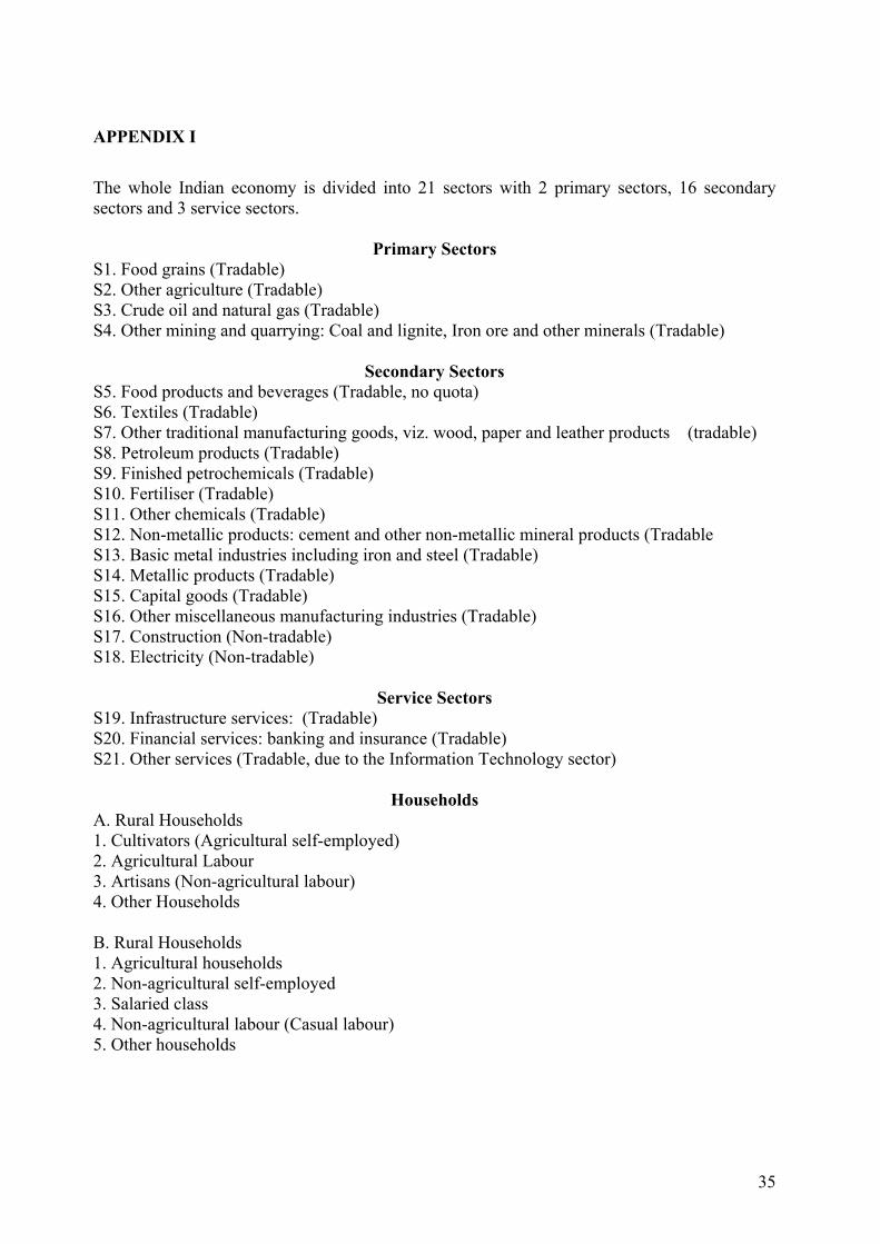
APPENDIX I

The whole Indian economy is divided into 21 sectors with 2 primary sectors, 16 secondary sectors and 3 service sectors.

Primary Sectors S1. Food grains (Tradable) S2. Other agriculture (Tradable) S3. Crude oil and natural gas (Tradable) S4. Other mining and quarrying: Coal and lignite, Iron ore and other minerals (Tradable)

Secondary Sectors S5. Food products and beverages (Tradable, no quota) S6. Textiles (Tradable) S7. Other traditional manufacturing goods, viz. wood, paper and leather products (tradable) S8. Petroleum products (Tradable) S9. Finished petrochemicals (Tradable) S10. Fertiliser (Tradable) S11. Other chemicals (Tradable) S12. Non-metallic products: cement and other non-metallic mineral products (Tradable S13. Basic metal industries including iron and steel (Tradable) S14. Metallic products (Tradable) S15. Capital goods (Tradable) S16. Other miscellaneous manufacturing industries (Tradable) S17. Construction (Non-tradable) S18. Electricity (Non-tradable)

Service Sectors S19. Infrastructure services: (Tradable) S20. Financial services: banking and insurance (Tradable) S21. Other services (Tradable, due to the Information Technology sector)

Households A. Rural Households 1. Cultivators (Agricultural self-employed) 2. Agricultural Labour 3. Artisans (Non-agricultural labour) 4. Other Households B. Rural Households 1. Agricultural households 2. Non-agricultural self-employed 3. Salaried class 4. Non-agricultural labour (Casual labour) 5. Other households

35

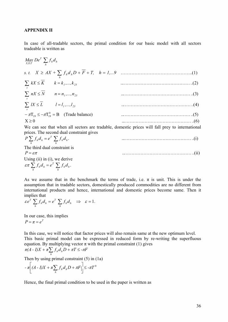
APPENDIX II

In case of all-tradable sectors, the primal condition for our basic model with all sectors tradeable is written as

∑h

hhT

TD,X,dfDeMax

s. t. 1,...9hT,FDdf +AXX h

hh =++≥ ∑ ………………………………………..(1)

)4(..

)3(..

)2(..

..l,...,llLlX

..n,...,nnNnX

..k,...,kkKkX

231s

231s

231s

………………………………………=≤

………………………………………=≤

………………………………………=≤

∑

∑

∑

)5(..)balanceTrade(BTT 01919 ..………………………………………=−≤− ππ

)6(..0X ..………………………………………≥ We can see that when all sectors are tradable, domestic prices will fall prey to international prices. The second dual constraint gives

)(i... ..dfedfPh

hhT

hhh ………………………………………= ∑∑

The third dual constraint is )(ii.. ..P ………………………………………= επ

Using (ii) in (i), we derive ∑∑ =

hhh

T

hhh dfedf .επ

As we assume that in the benchmark the terms of trade, i.e. π is unit. This is under the assumption that in tradable sectors, domestically produced commodities are no different from international products and hence, international and domestic prices become same. Then it implies that

∑∑ =⇒=h

hhT

hhh

T dfedfe .1εε

In our case, this implies

TeπP == In this case, we will notice that factor prices will also remain same at the new optimum level. This basic primal model can be expressed in reduced form by re-writing the superfluous equation. By multiplying vector π with the primal constraint (1) gives

F-TDdfπI)X-π(Ah

hh ππ ≤++ ∑

Then by using primal constraint (5) in (1a) 0T-FDdfπI)X-(Aπ-

hhh ππ ≤

++ ∑

Hence, the final primal condition to be used in the paper is written as

36

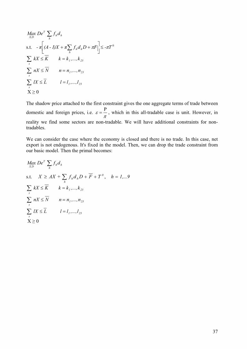
∑h

hhT

DX,dfDeMax

s.t. - 0T-FDdfπI)X-(Aπh

hh ππ ≤

++ ∑

231s

231s

231s

l,...,llLlX

n,...,nnNnX

k,...,kkKkX

=≤

=≤

=≤

∑

∑

∑

X ≥ 0 The shadow price attached to the first constraint gives the one aggregate terms of trade between

domestic and foreign prices, i.e. π

ε P= , which in this all-tradable case is unit. However, in

reality we find some sectors are non-tradable. We will have additional constraints for non-tradables. We can consider the case where the economy is closed and there is no trade. In this case, net export is not endogenous. It's fixed in the model. Then, we can drop the trade constraint from our basic model. Then the primal becomes:

∑h

hhT

DX,dfDeMax

s.t. 1,...9hTFDdf +AXX 0

hhh =++≥ ∑ ,

231s

231s

231s

l,...,llLlX

n,...,nnNnX

k,...,kkKkX

=≤

=≤

=≤

∑

∑

∑

X ≥ 0

37