Embed Size (px)
Citation preview

Impact of energy efficiency and renewable energy on electricity master
planning and design parameters
JA Alberts
11223871
Dissertation submitted in fulfilment of the requirements for the degree Master of Engineering in Electrical and Electronic
Engineering at the Potchefstroom Campus of the North-West University
Supervisor: Prof JA de Kock
May 2017

i
Preface
I am a director and professional engineer at a consulting engineering firm and liaise with clients
on a continuous basis, while also guiding staff in the execution of projects to meet client needs.
This research topic was selected based on the following considerations:
• the present working environment as a consulting electrical engineer;
• experience gained to date;
• a curiosity for the underlying interdependency of planning and design parameters
including the assumptions we make when planning future networks;
• a changing environment brought about by an increased drive for energy efficiency and the
implementation of renewable energy projects;
• a vision that the industry, especially the South African electricity distribution network
sphere at municipal and Eskom distribution level, requires a pro-active approach to deal
with this changing environment;
• my opinion that the industry may be tampering unknowingly with past assumptions without
revisiting and revising those assumptions, especially in terms of future load forecasting
and past designed and installed networks, while venturing into a new and unknown
territory; and
• my opinion that we may have already done so through existing initiatives.
I delivered a paper at the AMEU convention in 2014 [1] during the early stages of this research
and I plan to publish more papers on completion of the work.
Acknowledgements
I would like to thank my wife and children for their patience and understanding over the past three
years. Without my wife’s support, I would not have found the time to complete this study.
A special word of thanks to some of my clients and work colleagues for listening to my ideas.
I would like to acknowledge my study leader, Prof de Kock, for his guidance during the study.
Lastly, I would like to give thanks to God for the talents he bestowed upon us, without which this
research would have been impossible.

ii
Abstract
At the core of network planning and designs, after diversity maximum demand (ADMD) is routinely
used to define network conditions at peak periods. This dissertation explores the impact of
distributed generation and energy efficient measures on the parameters used in the planning and
design of residential distribution networks through an appliance-based load profile simulation and
load flow studies.
Traditionally, low voltage networks are operated radially in South Africa and the power flow
direction is from the utility source to the customer load. Networks are designed for compliance
with the lower end of the voltage regulation requirement (0.9 per unit) and to ensure that currents
do not exceed transformer capacity, cable or line ratings. With distributed generation, especially
when the load is low and generation is not restricted, voltage may rise and the power flow direction
may be reversed so that it flows towards the utility source. Not all utilities have policies in place,
and in many instances, distributed generation is implemented by households without knowledge
of the utility.
Methods to determine ADMD when it is not directly calculated through measurement of the
maximum demand, involves using a load factor and estimated energy consumption, or the
application of coincidence factors to individual household maximum demand. Load factor, as seen
by the utility, generally reduces when energy is generated during periods not coinciding with peak
demand, for example when electricity is generated by photo voltaic panels in a predominantly
evening-peak network. Off-peak generation will result in lower load factor and energy
consumption. When the utility is unaware of the distribution generation embedded in the network
and the ADMD is calculated using the load factor and energy consumption method and, the
calculated ADMD will be lower than required for design purposes of similar areas. Similarly, too
much distributed generation increases the coincidence factors. Increased coincidence factors
indicate a lack of diversity, which may result in a reverse ADMD higher than the original ADMD
for which the network was designed. This may lead to previously acceptable networks no longer
complying with regulations.
Key terms
Distributed generation, after diversity maximum demand, ADMD, reverse power flow

iii
Opsomming
Na-verskeidenheid maksimum-aanvraag (NVMA) vorm die kern van beplannings- en
ontwerpberekeninge om die netwerktoestande tydens piektye te definieer. Hierdie verhandeling
ondersoek die impak wat hernieubare energie en energie-effektiwiteitsmetodes het op die faktore
en aannames wat gebruik word tydens beplanning en ontwerp van residensiële kragnetwerke
deur middel van toestelgebaseerde lasprofielsimulasie en lasvloeistudies.
Laagspanningsnetwerke in Suid-Afrika word histories as radiale netwerke bedryf en die
drywingsvloeirigting is vanaf die voorsieningsowerheidsbron na die verbruikerslas. Derhalwe
word netwerke ontwerp om te voldoen aan die onderste grens van die spanningsregulasievereiste
(0.9. per eenheid) en om te verseker dat stroomwaardes nie die transformator-, kabel- of
lynvermoëns oorskry nie. Wanneer die las laag is en kragopwekking nie beperk word nie, kan die
spanning styg en die drywingsvloeirigting omkeer sodat dit in die rigting van die
voorsieningsowerheidsbron vloei. Nie alle voorsieningsowerhede het beleide in plek nie, en in
baie gevalle implementeer huishoudings verspreide opwekking sonder die medewete van die
voorsieningsowerheid.
Metodes om NVMA te bepaal wanneer dit nie direk bereken kan word deur middel van meting
van die maksimum-aanvraag nie, behels die gebruik van lasfaktor en energieverbruik, of die
toepassing van gelyktydigheidsfaktore en individuele maksimum aanvraag. In ʼn netwerk met ʼn
dominerende aandpiek vind die kragopwekkingspiek vir sonkrag plaas wanneer die las laag is. In
so ‘n netwerk verminder die lasfaktor en die energieverbruik, terwyl die gelyktydigheidsfaktore
onder sommige omstandigehde kan verhoog as gevolg van ‘n gebrek aan diversiteit tussen
generators. Die NVMA berekening deur middel van ‘n lasfaktor aanname en
energieverbruiklesings lewer ʼn laer waarde as wat dit werklik tydens die aandpiek is, omdat
kragopwekking deur middel van die son nie noodwendig die aandpiek verminder nie. Waar daar
geen beperking op kragopwekking geplaas word nie en meer krag word opgewek as wat die las
benodig, vloei krag terug na die voorsieningsowerheid. Onder sekere omstandighede kan daar
selfs meer krag terugvloei na die voorsieningsowerheid as waarvoor die netwerk ontwerp was,
en die netwerk sal nie meer aan die regulasies voldoen nie.
Sleutelterme
Verspreide generasie, na-verskeidenheid maksimum-aanvraag, NVMA, terugwaartse
drywingsvloei

iv
Table of Contents
Preface ........................................................................................................................................i
Acknowledgements .....................................................................................................................i
Abstract ...................................................................................................................................... ii
Key terms ................................................................................................................................... ii
Opsomming ............................................................................................................................... iii
Sleutelterme .............................................................................................................................. iii
Table of Contents ...................................................................................................................... iv
List of Tables ............................................................................................................................. xi
List of Figures .......................................................................................................................... xiii
Abbreviations ......................................................................................................................... xvii
Definitions .............................................................................................................................. xvii
Chapter 1: Background............................................................................................................ 19
Introduction .................................................................................................... 19
Energy efficiency and demand side management ....................................... 19
Renewable energy generation, embedded generation and distributed
generation ....................................................................................................... 21
Research questions ........................................................................................ 23
Research objective ......................................................................................... 24
Hypothesis ...................................................................................................... 24
Research methodology and approach .......................................................... 25
Dissertation structure .................................................................................... 27
Chapter 2 Literature study ................................................................................................. 29

v
Overview ......................................................................................................... 29
Theory: planning parameters ........................................................................ 31
2.2.1 Overview .......................................................................................................... 31
2.2.2 Load profile ....................................................................................................... 32
2.2.3 Load factor ....................................................................................................... 33
2.2.4 ADMD ............................................................................................................... 34
2.2.5 Demand factor, coincidence and diversity ......................................................... 39
2.2.6 Unbalance and diversity correction factors ....................................................... 42
2.2.7 Relationship between coincidence and load factor ........................................... 43
2.2.8 Load loss factor ................................................................................................ 46
2.2.9 Load growth ...................................................................................................... 47
2.2.10 LV feeder design methods ................................................................................ 50
Design and planning parameters informed by law, regulations,
standards and guidelines in South Africa..................................................... 50
2.3.1 Overview .......................................................................................................... 50
2.3.2 Grid code .......................................................................................................... 51
2.3.3 Standards and specifications overview ............................................................. 53
2.3.4 NRS 048: Quality of supply ............................................................................... 53
2.3.5 SANS 507 / NRS 034 ....................................................................................... 53
2.3.6 NRS 097 ........................................................................................................... 57
2.3.7 SANS 10142 ..................................................................................................... 59
2.3.8 Planning Guidelines - overview ......................................................................... 60
2.3.9 Guideline for Human Settlement Planning ........................................................ 61

vi
2.3.10 Parameters for non-domestic load .................................................................... 62
2.3.11 DGL 34-431 Eskom Methodology for Network Master Plans and Network
Development Plans .......................................................................................... 63
2.3.12 DGL 34-1284 Geo-based Load Forecast Guideline .......................................... 64
Impact of historic EEDSM initiatives ............................................................. 65
Distributed generation ................................................................................... 66
2.5.1 Overview .......................................................................................................... 66
2.5.2 European case study ........................................................................................ 67
2.5.3 Benefits of introducing DG ................................................................................ 69
2.5.4 Grid problems introduced by DG....................................................................... 69
2.5.5 Impact of uncontrolled actions .......................................................................... 74
2.5.6 Solutions proposed in the literature ................................................................... 74
Chapter summary ........................................................................................... 75
Chapter 3 Analysis and modelling ..................................................................................... 77
Review of the findings from the literature study .......................................... 77
Review of research questions and basic approach ..................................... 77
3.2.1 RQ4, 7, 8: Relationship between diversity and load factor, impact on ADMD
and traditional diversity factors ......................................................................... 77
3.2.2 RQ5, 6, 9, 10: Solar PV impact on LV and MV network performance,
system losses and fault levels .......................................................................... 78
3.2.3 Approach summary .......................................................................................... 78
Load profile simulation .................................................................................. 78
3.3.1 General considerations ..................................................................................... 78
3.3.2 Load profile composition ................................................................................... 79

vii
3.3.3 Appliance load profile considerations ................................................................ 80
3.3.4 Algorithm to calculate a load profile based on appliances per household.......... 80
3.3.5 Parameters that can be calculated from the constructed load profiles .............. 82
Matrices required to simulate the appliance model ..................................... 82
Application of matrices / vectors to develop the profile .............................. 84
3.5.1 Household type ................................................................................................. 84
3.5.2 Households ...................................................................................................... 85
3.5.3 Appliance list .................................................................................................... 85
3.5.4 Appliances per household type ......................................................................... 85
3.5.5 Appliances active per household ...................................................................... 87
3.5.6 Appliance_Probability_On ................................................................................ 90
3.5.7 Appliance_Minute_Start .................................................................................... 90
3.5.8 Appliance_Minute_On and Appliance_Load_Minute ......................................... 90
3.5.9 Appliance_Summated_Profile_Minute, T and Total_Domestic_Profile .............. 91
3.5.10 Typical “per-minute” appliance profiles generated ............................................ 91
3.5.11 Total profile generated ...................................................................................... 92
Base model validation .................................................................................... 92
Introducing energy efficiency and renewable energy measures ................ 93
3.7.1 Solar PV curve .................................................................................................. 93
3.7.2 Gas-cooking – stove-top ................................................................................... 94
3.7.3 Gas-cooking - oven .......................................................................................... 94
3.7.4 Load shifting ..................................................................................................... 95
3.7.5 Load reduction .................................................................................................. 95

viii
3.7.6 Adjusted profile calculation ............................................................................... 95
3.7.7 Study case generation ...................................................................................... 96
Load flow model ............................................................................................. 97
3.8.1 Load flow model requirements .......................................................................... 97
3.8.2 Load flow model design .................................................................................... 98
3.8.3 Load flow modelling scenarios ........................................................................ 102
Chapter summary ......................................................................................... 103
Chapter 4 Findings and results........................................................................................ 104
Introduction .................................................................................................. 104
Load profile validation and verification ...................................................... 104
4.2.1 General considerations ................................................................................... 104
4.2.2 Load profile shape .......................................................................................... 105
4.2.3 ADMD ............................................................................................................. 107
4.2.4 Diversity / Coincidence ................................................................................... 108
4.2.5 Load factor ..................................................................................................... 109
4.2.6 Effect of “green” measures ............................................................................. 110
4.2.7 Validation and verification conclusion ............................................................. 110
Analysis of results obtained through appliance model simulation ........... 110
4.3.1 Case studies ................................................................................................... 110
4.3.2 Impact of green measures on ADMD .............................................................. 111
4.3.3 Impact of green initiatives on coincidence ....................................................... 114
4.3.4 Impact of green initiatives on load factor ......................................................... 116
4.3.5 Summary of initiatives and interdependent impact .......................................... 118

ix
4.3.6 Analysis of the distribution of peak current ...................................................... 123
Load flow analysis ........................................................................................ 126
4.4.1 Analysis presented previously ........................................................................ 126
4.4.2 Baseline analysis ............................................................................................ 127
4.4.3 Comparison of results with different DG control algorithms: voltage ............... 131
4.4.4 Comparison of results with different DG control algorithms: current ................ 132
4.4.5 Comparison of results with different DG control algorithms: total power flow .. 138
Chapter summary ......................................................................................... 140
Chapter 5 Conclusion ...................................................................................................... 141
Load profile modelling conclusion .............................................................. 141
Load flow study conclusion ......................................................................... 141
Summarized conclusion............................................................................... 142
Review of research questions and associated findings ............................ 144
Review of findings against original hypothesis ......................................... 145
Chapter 6 Recommendation for further study / work ....................................................... 148
Simulation model .......................................................................................... 148
Reactive power and power factor ................................................................ 149
Protection ...................................................................................................... 149
Thermal cycling ............................................................................................ 149
REFERENCES ...................................................................................................................... 150
Appendix A: Appliance model load simulation tool: User Interface ........................................ 154
Overview ....................................................................................................... 154
7.1.1 User interface outline ...................................................................................... 154

x
7.1.2 Application usage ........................................................................................... 154
7.1.3 Application routines ........................................................................................ 155
Profile tab: The main user interface (UI) sub-tab........................................ 158
7.2.1 Main components ........................................................................................... 158
7.2.2 Button functions .............................................................................................. 160
7.2.3 Input variables ................................................................................................ 160
Profile tab: Total load profile data ............................................................... 160
Profile tab: Graphs sub-tab .......................................................................... 162
Profile tab: Study cases ............................................................................... 163
Profile tab: Sorted study case ..................................................................... 164
Hourly tables ................................................................................................. 165
7.7.1 Appliance Present .......................................................................................... 165
7.7.2 Appliance Active ............................................................................................. 167
7.7.3 Appliance load (kW)........................................................................................ 168
7.7.4 Appliance “On” Duration (Minutes) .................................................................. 169
MINUTE TABLES .......................................................................................... 170
7.8.1 Households .................................................................................................... 170
7.8.2 Appliance_Probability_On .............................................................................. 171
7.8.3 Appliance_Minute_Start .................................................................................. 172
7.8.4 Appliance_Minute_On .................................................................................... 173
7.8.5 Appliance_Load_Minute ................................................................................. 174
7.8.6 Profile per household (T) ................................................................................ 175
EE/DSM Green measures ............................................................................. 176

xi
List of Tables
Table 1-1: Methodology to investigate respective research questions .................................... 26
Table 2-1: Master planning process – alternatives (Source: [2], [6]) ........................................ 30
Table 2-2: Diversity factors as tabled by the Standard Handbook for Electrical Engineers,
Table 18-26 [15] .................................................................................................... 40
Table 2-3: Peak contribution of non-domestic loads (Source: Eskom [10], table in par
3.1b) ...................................................................................................................... 41
Table 2-4: Historical empirical diversity correction and unbalance correction factors used
in South Africa, available with ReticMaster simulation software ............................. 42
Table 2-5: South African Grid Code components..................................................................... 51
Table 2-6: NRS 034-recommended Herman-Beta parameters for various income classes
for residential load estimation – 15-year forecast values [3] .................................. 56
Table 2-7: Allowable LV DG connections (individual limits) [29], [30] ....................................... 58
Table 2-8: SANS 10142-1 Coincidence factors for residential units [31] .................................. 59
Table 2-9: Neutral unbalance multiplication factors for calculating volt drop (refer to [31]
Table E3) .............................................................................................................. 60
Table 2-10: Consumption classes (refer to [8] table 12.1.1) ..................................................... 61
Table 2-11: Consumption classes (refer to [10] table 3) ........................................................... 61
Table 2-12: Domestic density classification ([8] table 12.1.2, [10] table 4) ............................... 62
Table 2-13: Maximum energy demand per building classification for each climatic zone
([33] table 1) .......................................................................................................... 62
Table 2-14: Maximum annual consumption per building classification for each climatic
zone in South Africa ([33] Table 2 ......................................................................... 63
Table 3-1: Matrices / Vectors used in profile calculation .......................................................... 83

xii
Table 3-2: Household type definition ....................................................................................... 84
Table 3-3: Household type characteristics, indicating number of occupants, age of
occupants, household size .................................................................................... 84
Table 3-4: Example of appliance presence, seasonality and appliance load rating .................. 86
Table 3-5: Example of the Appliance_Active matrix ................................................................. 88
Table 3-6: Simplified solar PV parabola coefficients ................................................................ 93
Table 4-1: Validation and verification methodology ................................................................ 104
Table 4-2: Study scenarios with appliance model simulation tool .......................................... 110
Table 4-3: Impact on parameters for simulations of 100 households or more ........................ 118
Table 4-4: Summary of impact to ADMD, coincidence and load factor due to
implementation of various green initiatives .......................................................... 122
Table 4-5: Distribution of peak currents under various scenarios ........................................... 123
Table 4-6: Load flow scenarios .............................................................................................. 126
Table 7-1: Matlab application file list ...................................................................................... 156
Table 7-2: Column headings related to time of the day .......................................................... 161

xiii
List of Figures
Figure 1-1:Typical daily load profile in Ghana for a typical 33 kV feeder over a randomly
selected period of 3 days inclusive of a weekend .................................................. 20
Figure 1-2: Traditional power flow ........................................................................................... 21
Figure 1-3: Power flow with smaller scale, distributed and embedded generation, with the
possibility of reverse power flow indicated ............................................................. 22
Figure 1-4: South African peak demand declines and Eskom tariff increases (derived from
tabular data published in the NERSA System Adequacy Outlook report – table
1 [4], and the Eskom Tariff Book [5]) ..................................................................... 22
Figure 2-1: Master planning and design in context .................................................................. 29
Figure 2-2: Eskom master planning methodology [2] ............................................................... 31
Figure 2-3: Typical load profiles, also illustrating the concept of composite load profiles ......... 32
Figure 2-4: Load factor defined (Source: Guideline for Human Settlement Planning) [8] ......... 33
Figure 2-5: Measurement error of the maximum demand of a 10 MVA network, expressed
as a percentage, as a result of integration over time compared to one-minute
measurements for (a) seven consecutive days and (b) one month ....................... 37
Figure 2-6: Diversity factors for a power system (derived from Table 2-2) ............................... 40
Figure 2-7: Bary's curve for various measurements of coincidence against load factor [13] ..... 44
Figure 2-8: Bary coincidence factors related to load factor [18] ............................................... 45
Figure 2-9: Growth S-curves illustrating variance in growth rate (calculated) ........................... 48
Figure 2-10: Example of growth curves with different future maximum demand ...................... 48
Figure 2-11: Example of a beta distribution curve that is left skewed ....................................... 55
Figure 2-12: NRS097 proposed limits of embedded generation (based on values
contained in [30]) ................................................................................................... 57
Figure 2-13: Effect of ripple control on maximum demand and ADMD [1] ................................ 65

xiv
Figure 2-14: Figures 1,3, 4 and 6 of Derlab Study indicating solar PV expansion per year
per EU country, network connectivity, penetration levels and German export
scenario respectively [34] ...................................................................................... 68
Figure 2-15: Fault currents during a fault with DG present [39] ................................................ 72
Figure 2-16: Effect on power factor through active power DG generation ................................ 73
Figure 2-17: Proposed solutions by an European study [34], table 10 ..................................... 75
Figure 3-1: Load profile appliance-based model algorithm ...................................................... 81
Figure 3-2: Typical appliance model extract ............................................................................ 91
Figure 3-3: Extract of appliance model applied to multiple households .................................... 92
Figure 3-4: Solar PV per unit curve.......................................................................................... 94
Figure 3-5: LV feeder configuration for load flow studies for tapered feeder (scenario A1)
and one size feeder (Scenario A2) [1] ................................................................... 99
Figure 3-6: Reticmaster model for test LV feeder network ..................................................... 100
Figure 3-7: Digsilent Powerfactory model for test LV feeder network ..................................... 101
Figure 4-1: Calculated load profile (black) compared to a reference curve (magenta) with
load control (sub-figure a) and without load control (sub-figure b) ....................... 106
Figure 4-2: ADMD vs number of households (simulated) ....................................................... 107
Figure 4-3: Coincidence vs number of households (simulated) .............................................. 108
Figure 4-4: Load factor vs number of households (simulated) ............................................... 109
Figure 4-5: Effect of various green measures on ADMD, compared to a baseline without
any interventions ................................................................................................. 112
Figure 4-6: ADMD change in number of households for green interventions relative to a
baseline without any form of intervention............................................................. 113
Figure 4-7: Percentage change in ADMD per number of households in the simulation
group relative to a baseline without any form of intervention ............................... 114

xv
Figure 4-8: Impact on coincidence for green interventions relative to a baseline without
any form of intervention ....................................................................................... 115
Figure 4-9: Percentage coincidence change for green interventions relative to a baseline
without any form of intervention ........................................................................... 116
Figure 4-10: Impact on load factor for green interventions relative to a baseline without
any form of intervention ....................................................................................... 117
Figure 4-11: Percentage change in load factor for green interventions relative to a
baseline without any form of intervention............................................................. 118
Figure 4-12: Impact of various green interventions: (a) ADMD change in kVA, (b) ADMD
% change, (c) Coincidence % change and (d) Load factor percentage change ... 120
Figure 4-13: Additional findings: (a) ADMD vs Load factor; (b) ADMD vs Coincidence; (c)
Coincidence vs Load factor ................................................................................. 121
Figure 4-14: Baseline Digsilent Powerfactory voltage profile for the red, white and blue
phases respectively along test feeder under high load conditions for a) tapered
feeder, and b) one-size feeder ............................................................................ 129
Figure 4-15: Baseline Digsilent Powerfactory voltage profile for the red, white and blue
phases respectively along test feeder under low load conditions for a) tapered
feeder, and b) one-size feeder ............................................................................ 130
Figure 4-16: Comparison of various inverter control methods and sizes for a) high load
conditions and b) low load conditions. Red arrows point to violation of voltage
limits. ................................................................................................................... 131
Figure 4-17: Cable loading (percentage of rated current for the highest loaded phase)
along feeder for the tapered feeder under high load conditions ........................... 132
Figure 4-18: Cable loading (percentage of rated capacity for the highest loaded phase) for
the one-size feeder under high load conditions ................................................... 133
Figure 4-19: Cable loading (percentage of rated capacity for the highest loaded phase)
along feeder for the tapered feeder under low load conditions. Scenarios
marked with a red dashed box failed on cable overloading. ................................ 134

xvi
Figure 4-20: Cable loading (percentage of rated capacity for the highest loaded phase) for
the one-size feeder under low load conditions. Scenarios marked with a red
dashed box failed on cable overloading............................................................... 135
Figure 4-21: Protection device arrangement for a tapered and one-size LV cable feeder ...... 136
Figure 4-22: Power flow conditions through the transformer for various load flow scenarios . 138
Figure 4-23: Power flow conditions through the transformer for various load flow scenarios . 139
Figure 5-1: 24-hour load profile with reverse power flow as a result of DG ............................ 143
Figure 7-1: Main User Interface (UI) screen / start-up screen ................................................ 159
Figure 7-2: One-minute calculated profile screen .................................................................. 161
Figure 7-3: Graphs screen ..................................................................................................... 162
Figure 7-4: Study cases sub-tab screen ................................................................................ 164
Figure 7-5: Sorted study cases sub-tab screen ..................................................................... 164
Figure 7-6: Appliance Present sub-tab screen ....................................................................... 165
Figure 7-7: Appliance Active sub-tab screen ......................................................................... 167
Figure 7-8: Appliance load sub-tab screen ............................................................................ 168
Figure 7-9: Appliance "On" duration sub-tab screen .............................................................. 169
Figure 7-10: Households sub-tab screen ............................................................................... 170
Figure 7-11: Appliance_Probability_On sub-tab screen ......................................................... 171
Figure 7-12: Appliance_Minute_Start sub-tab screen ............................................................ 172
Figure 7-13: Appliance_Minute_On sub-tab screen ............................................................... 173
Figure 7-14: Appliance_Load_Minute sub-tab screen ............................................................ 174
Figure 7-15: Profile per household (T Matrix) sub-tab screen ................................................ 175
Figure 7-16: Appliance modify sub-tab screen ....................................................................... 176

xvii
Abbreviations
ADMD After diversity maximum demand
DG Distributed Generation
EEDSM Energy Efficiency and Demand Side Management
EHV Extra High voltage
HV High voltage
LV Low voltage
MV Medium voltage
RPP Renewable Power Plants
SADC South African Distribution Code
SAGC South African Grid Code
Definitions
Embedded generator / Distributed generator
A grid-tied generator over which the system operator has no dispatching control because it is
embedded in a customer’s network, such as a solar roof-top photo voltaic system, or a diesel
generator set.
Small-scale renewable energy
Energy generation through solar, wind, biomass or any other form of renewable energy smaller
than or equal to 100 kW.
System operator
The party responsible for dispatching electricity from generators belonging to licensed generators,
whether national or as independent power producers

xviii
Extra High voltage
A voltage (Un) exceeding 220 kV1
High voltage
A voltage (Un) exceeding 44 kV, but not exceeding 220 kV2
Medium voltage
A voltage (Un) exceeding 1000 V, but not exceeding 44 kV3
Low voltage
A voltage (Un) not exceeding 1000 V4
.
1 According to SANS 1019 of 2001 and the South African Grid Code. 2 According to SANS 1019 of 2001 and the South African Grid Code. The South African Grid Code for
RPPs indicate the lower limit as 33kV 3 According to SANS 1019 of 2001 and the South African Grid Code. The South African Grid Code for
RPPs indicate the upper limit as 33kV 4 According to SANS 1019 of 2001

19
Chapter 1: Background
Introduction
Throughout the world there is a drive to improve energy efficiency, to reduce electricity demand
and to encourage renewable energy generation. Various sources inform the public that this is
good for the environment, will prolong generation and grid assets and natural resources such as
fossil fuels and water. However, it may be possible that these initiatives change the performance
of planned (future) and designed (existing) networks without engineers reconsidering past
assumptions or traditional design methods.
In electricity distribution network master planning and designs, the planner or designer must make
various assumptions while considering future loading and scenarios. The planning window is
generally 20 years for master planning [2] and 15 years for electrification planning [3]. A few
factors stand out in such planning exercises, namely diversity factors, load factors, load profiles,
loss factors, growth rate and after diversity maximum demand (ADMD). Several assumptions are
made in the selection of suitable parameters and combinations of parameters to predict future
load and to plan and design infrastructure accordingly. If parameters are affected and the impact
of a change is not considered, unexpected or even degraded performance of networks may result,
while utilities and municipal electricity re-sellers may have to lay out unplanned capital to rectify
or address the resulting problems.
Energy efficiency and demand side management
A recorded load profile for a 33 kV feeder in Ghana in 2011 (refer to Figure 1-1 below) revealed
that the typical daily load profile has a load factor of approximately 80%. From a South African
perspective, typical municipal load factors are approximately 50%. The Ghana feeder supplies
predominantly residential customers with negligible commercial and industrial activity. Residential
load factors in South Africa are lower than 50%. The high load factor and load profile shape raised
questions about typical coincidence factors to be used for future load estimates while planning
two new cities in Ghana.

20
It was observed while visiting Ghana in 2011 and 2012 that electricity is neither used for water
and space heating, nor for cooking. Standby loads are usually switched off after use (e.g.
televisions and cell phone chargers) due to the high cost of electricity and limited supply. It
therefore appears that climate and consumer behaviour will affect a load profile, which is reflected
in the load factor. This poses a few questions, namely:
• Does a more efficient use of electricity, or a use influenced by behavioural change improve
load factor?
• If it does, how does it change coincidence factors? In other words, is there a relationship
between coincidence and load factor?
Another observation was that a ripple relay installation increases the maximum demand of a 45
MVA transformer from 42 MVA to 47 MVA. The new peak was due to the so-called “cold pick-up”
load stage occurring when ripple relays switch hot water cylinders back on. The ADMD of the
network increases and the load profile shape changes because the controlling algorithm is not
properly configured to prevent such a scenario. Apart from the transformer, which is loaded in its
emergency loading range for a short period every 24 hours, it is possible that network MV and LV
feeders operate under stress or under overloaded conditions, while voltage drop limits could be
0
1
2
3
4
5
6
7
8
9
10
00
:00
01
:00
02
:00
03
:00
04
:00
05
:00
06
:00
07
:00
08
:00
09
:00
10
:00
11
:00
12
:00
13
:00
14
:00
15
:00
16
:00
17
:00
18
:00
19
:00
20
:00
21
:00
22
:00
23
:00
De
man
d (
MV
A)
33 kV feeder load profile for period 6 to 8 Aug 2011
Sa 2011/08/06
Su 2011/08/07
Mo 2011/08/08
Time of day
Figure 1-1:Typical daily load profile in Ghana for a typical 33 kV feeder over a
randomly selected period of 3 days inclusive of a weekend
21
exceeded. This is a good example of a DSM initiative that has changed a designed network and
that would have rendered future load forecasts insufficient.
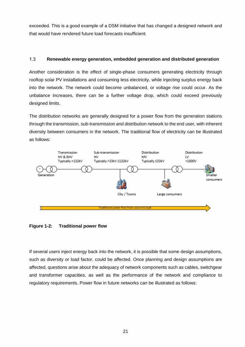
Renewable energy generation, embedded generation and distributed generation
Another consideration is the effect of single-phase consumers generating electricity through
rooftop solar PV installations and consuming less electricity, while injecting surplus energy back
into the network. The network could become unbalanced, or voltage rise could occur. As the
unbalance increases, there can be a further voltage drop, which could exceed previously
designed limits.
The distribution networks are generally designed for a power flow from the generation stations
through the transmission, sub-transmission and distribution network to the end user, with inherent
diversity between consumers in the network. The traditional flow of electricity can be illustrated
as follows:
Figure 1-2: Traditional power flow
If several users inject energy back into the network, it is possible that some design assumptions,
such as diversity or load factor, could be affected. Once planning and design assumptions are
affected, questions arise about the adequacy of network components such as cables, switchgear
and transformer capacities, as well as the performance of the network and compliance to
regulatory requirements. Power flow in future networks can be illustrated as follows:

22
~
TransmissionHV & EHVTypically >132kV
DistributionMVTypically ≤33kV
DistributionLV<1000V
Sub-transmissionHVTypically >33kV ≤132kV
Generation
City / Towns Large consumers
Smaller consumers
Traditional power flow from source to load
~
Large scale renewable energy
generation
~
Medium scale renewable energy
generation
Smaller scale generated power flows according to impedance of network and load required
Figure 1-3: Power flow with smaller scale, distributed and embedded generation, with
the possibility of reverse power flow indicated
When considering the South African peak demand, a decline in the annual demand since 2007 is
observed:
Figure 1-4: South African peak demand declines and Eskom tariff increases (derived
from tabular data published in the NERSA System Adequacy Outlook report – table 1 [4],
and the Eskom Tariff Book [5])
100
200
300
400
500
600
700
31000
32000
33000
34000
35000
36000
37000
2007 2008 2009 2010 2011 2012 2013 2014 2015
An
nu
al E
sko
m t
arif
f in
crea
se(2
007
= b
ase
of 1
00)
Pea
k d
eman
d (M
W)
Year
South African annual peak demand versus tariff increases
Peak demand (MW) Total tariff increase

23
The decline may be attributed to a decline in economic activity, rising electricity costs and the
rapid expansion of renewables. In 2008, load shedding took place, which resulted in an abnormal
decline in peak demand. Electricity costs in South Africa have risen with 637% since 2007
(calculated from electricity increases published by Eskom [5]). The rapid expansion of renewables
emphasizes the need to study the impact this technology will have on the South African networks.
Research questions
The questions that are investigated in this study, are:
(1) Which planning and design parameters are affected by EEDSM initiatives and small-scale
renewable energy generation?
(2) How are these parameters affected?
(3) Is there an interdependency between these parameters, and if so, how sensitive would a
change in one or more parameters be to other interdependent parameters?
Questions 2 and 3 above can be considered in lieu of the following questions:
(4) What is the relationship between coincidence or diversity and load factor?
(5) How does single-phase injection on the low voltage network affect the low voltage network’s
performance and integrity?
(6) How does generation from LV and MV embedded/distributed generation in general affect
the network up- and downstream from the point of generation?
(7) How will ADMD factors be influenced by EEDSM and renewable energy generation at low
voltage level / distributed generation?
(8) How are traditional diversity factors between LV feeders, transformers on medium voltage
feeders, feeders at a substation and further upstream networks affected?
(9) How are system losses affected when load profiles are altered through EEDSM initiatives
and reverse power flow due to renewable energy generation?

24
(10) How are fault-levels affected by renewable energy injection on the low voltage, medium
voltage and high voltage networks respectively, and what is the impact on protection
systems and equipment ratings?
The study excludes the following:
• impact on utility revenue streams,
• impact on health and safety, and
• impact on power quality.
Research objective
The objective is to investigate the impact, if any, on electricity network planning and design
parameters and factors when energy efficiency, demand side management or renewable energy
projects are implemented. In other words, are original planning and design assumptions still valid
after implementation of EEDSM measures or renewable energy, or is there risk that “green
measures” may affect the grid negatively?
Hypothesis
The following is postulated:
• Energy efficiency generally reduces the system peak and therefore ADMD. Technical losses
will also be reduced.
• Load shifting techniques, when not properly controlled, can increase the ADMD, especially if
the load is associated with thermal storage.
• Improving the load factor reduces the diversity of similar load class consumers.
• Reducing the diversity of consumers will impact designed and constructed networks by
increasing the voltage drop experienced by consumers. However, the reduced energy
consumption and demand could mean that the effect is cancelled out or reduced.
• Uncontrolled solar PV injection into the network may cause network unbalance, which will
affect a voltage drop in designed and constructed networks. LV networks are designed for a
diversified power flow in one direction. A reverse power flow in a high penetration solar PV

25
network, producing excess energy during solar peak, will exceed the power a LV feeder can
handle due to a lack of diversity during reverse power flow.
Research methodology and approach
The research entailed a literature review and simulations and calculations. A literature study was
conducted to:
• review the basic regulatory requirements for planning compliance in South Africa and any
prescribed parameters;
• review the planning standards applicable in South Africa;
• review theory;
• review historic and present methods for distribution network planning and design; and to
• review research conducted in the specific field.
On completion of the literature review, the research questions were further investigated by
creating a load profile simulation and a load flow simulation model of a representative network.
Parameters will be varied to determine impact, sensitivity as well as interdependency.
The methodology can be outlined as follows:

26
Table 1-1: Methodology to investigate respective research questions
ITEM RESEARCH QUESTION METHODOLOGY TO INVESTIGATE
RQ4 What is the relationship
between diversity and load
factor?
An analysis of the various formulae for the
various parameters. This also involved an
analysis of the summation of individual load
profile curves per load class, with load
factors per load class.
The aim was to determine whether diversity
is affected by changes in load profile. This
was examined by considering e.g. ripple
control demand side management altered
profiles, subtracting solar PV renewable
energy superimposed profiles and solar
thermal water heating effects, gas cooking
etc.
RQ5 How does single-phase
injection on the low voltage
network affect the low voltage
network’s performance and
integrity?
Simulate by means of a network model for a
typical designed network.
RQ6 How does generation from LV
and MV embedded/distributed
generation in general affect the
network up- and downstream
from the point of generation?
Simulate by means of a network model.
RQ7 How will ADMD factors be
influenced by energy efficiency
and renewable energy
generation at low voltage level?
Perform calculations on load profiles, and
supplement with load profiles from recently
commissioned solar farms, NWU-measured
data or simulated data.

27
ITEM RESEARCH QUESTION METHODOLOGY TO INVESTIGATE
RQ8 How are traditional diversity
factors affected between LV
feeders, transformers on MV
feeders, between feeders at a
substation and further
upstream?
Detailed load data on 132 kV, 66 kV and 11
kV MV feeder level are available from a
recent master plan study. This can be used
to model diversity factors at various levels,
compare with literature, international and
South African “experience” values, where
after profile changes can be applied.
RQ9 How are system losses
affected by load profiles altered
by energy efficiency and
reverse power flow due to
renewable energy generation?
Assess loss factor through its relationship to
technical (I2R) losses, its link to load factor
and its link to diversity and changes to load
profiles and these parameters.
RQ10 How are fault levels affected by
renewable energy injection on
the low voltage, medium
voltage and high voltage
networks respectively, and
what is the impact on protection
systems and equipment
ratings?
Fault levels would generally increase at the
point of power injection. The point at which it
injects relative to previously existing critical
elements and protection systems will be
evaluated.
Dissertation structure
The dissertation is structured as follows:
• Preface
• Abstract
• Chapter 1: Introduction - In this chapter the reader is introduced to the problem, the research
questions, the hypothesis and the proposed research methodology.

28
• Chapter 2: Literature Study - This chapter includes a review of local regulatory frameworks
and standards as far as planning parameters are concerned, a review of theory and a review
of review of research already conducted concerning the research questions.
• Chapter 3: Analyses and modelling - This chapter discusses the models generated, any data
sets used and the analyses conducted.
• Chapter 4: Findings and results - This chapter documents the findings of all the simulations
and analysis.
• Chapter 5: Conclusion
• Chapter 6: Recommendation for further studies / work - Should the research indicate that past
assumptions are impacted and that design and planning methods or parameters have to
change, this chapter offers recommendations for further investigation into new planning or
design methods.
• Bibliography
• Appendices

29
Chapter 2 Literature study
Overview
A holistic understanding of the planning and design processes is crucial prior to investigating each
aspect in more detail.
Eskom Distribution has provided a methodology for network master plans (NMPs) and network
development plans (NDPs) under document number DGL 34-431 [2]. The NMP is the long-term
plan with a 20-year horizon, while the NDP focuses on shorter horizons – typically five years.
Shorter horizons (two to three years) are labelled as project planning.
Graphically, considering Figure 1-3, the master planning and design scope can be illustrated in
Figure 2-1:
~
TransmissionHV & EHVTypically >132kV
DistributionMVTypically ≤33kV
DistributionLV<1000V
Sub-transmissionHVTypically >33kV ≤132kV
Generation
City / Towns Large consumers
Smaller consumers
Traditional power flow from source to load
~
Large scale renewable energy
generation
~
Medium scale renewable energy
generation
Smaller scale generated power flows according to impedance of network and load required
Traditionally, municipalities in South Africa do not separate their master plans into multiple
studies, but compile the short, medium and long-term plans as part of one master plan study.
Generation and
Transmission master plan
Distribution master plan
(NMP & NDP)
Distribution master plan
(NDP)
LV feeder
design *
Figure 2-1: Master planning and design in context
Designed during Generation or Transmission project
implementation
MV design during Distribution
project implementation
Excluded from
master planning

30
Consulting engineers mostly execute these studies for municipalities and they lately follow the
same methodology as Eskom.
H. Lee Willis explains the evaluation of alternatives for the master planning process in general
[6], while Eskom [2] incorporated problem identification and goals with the evaluation of
alternatives (see table 2-1):
Table 2-1: Master planning process – alternatives (Source: [2], [6])
Willis also outlines a spatial approach to load forecasting [7] and Eskom has considered the
international best practice outlined by Willis and refined it further for their needs [2]. Figure 2-2
illustrates the Eskom master planning process (which is generally accepted as best practice in
South Africa):

31
Figure 2-2: Eskom master planning methodology [2]
Using Figure 2-2 as a frame of reference, the master planning areas covered by this dissertation
are:
• 5.3: Load (MD) profiles
• 5.4: Demand & Energy forecast (Load forecast in the diagram refers to the geographic location
of the load and type of load)
The LV feeder design parameters are discussed in their entirety, as this is where most small scale
distributed and embedded generation may have an impact. LV feeder, MV feeder and MV/LV
transformer design involve the sizing of conductors to transfer the required load while maintaining
the voltage within limits, sizing of transformers and other equipment, and protection and earthing
arrangements. Earthing and protection arrangements are not discussed in this dissertation,
except for fault level implications, or where power quality aspects caused by small scale
distributed or embedded generation have an impact on energy and demand aspects.
Theory: planning parameters
2.2.1 Overview
Planning parameters refer to certain parameters required to do planning. Planning involves the
sizing of equipment based on future loading requirements. Knowledge of planning parameters
and how they relate to one another makes it possible to assess the impact new industry initiatives

32
such as deploying DG or changing electrical geysers with solar geysers will have on past
assumptions. It also provides guidance on how future thinking should change.
2.2.2 Load profile
The network’s load profile is the sum of individual load class load profiles.
Figure 2-3: Typical load profiles, also illustrating the concept of composite load profiles
The residential and commercial load class load profiles in Figure 2-3 summate to produce the
total load profile. The commercial load profile peaks around noon, while the residential profile
peaks in the morning and the evening, but with the evening peak being the highest. When the two
profiles are summated, the new peak is neither in the afternoon, nor in the evening, but rather in
the morning.
Figure 2-3 shows the apparent demand in kVA. When the demand is shown in kW, the area under
the line is the energy consumption. The load factor can be determined from the load profile if the
maximum demand and the average demand are known, or if the maximum demand and the
energy consumption are known.
0
200
400
600
800
1000
1200
1400
1600
1 2 3 4 5 6 7 8 9 10 11 12 13 14 15 16 17 18 19 20 21 22 23 24
Dem
and
(kV
A)
Time of day in hours
Typical winter day profile
6A commerce retail winter weekday UrbEst 10h+ winter weekday Total winter weekday
C=A+B
B
A
33
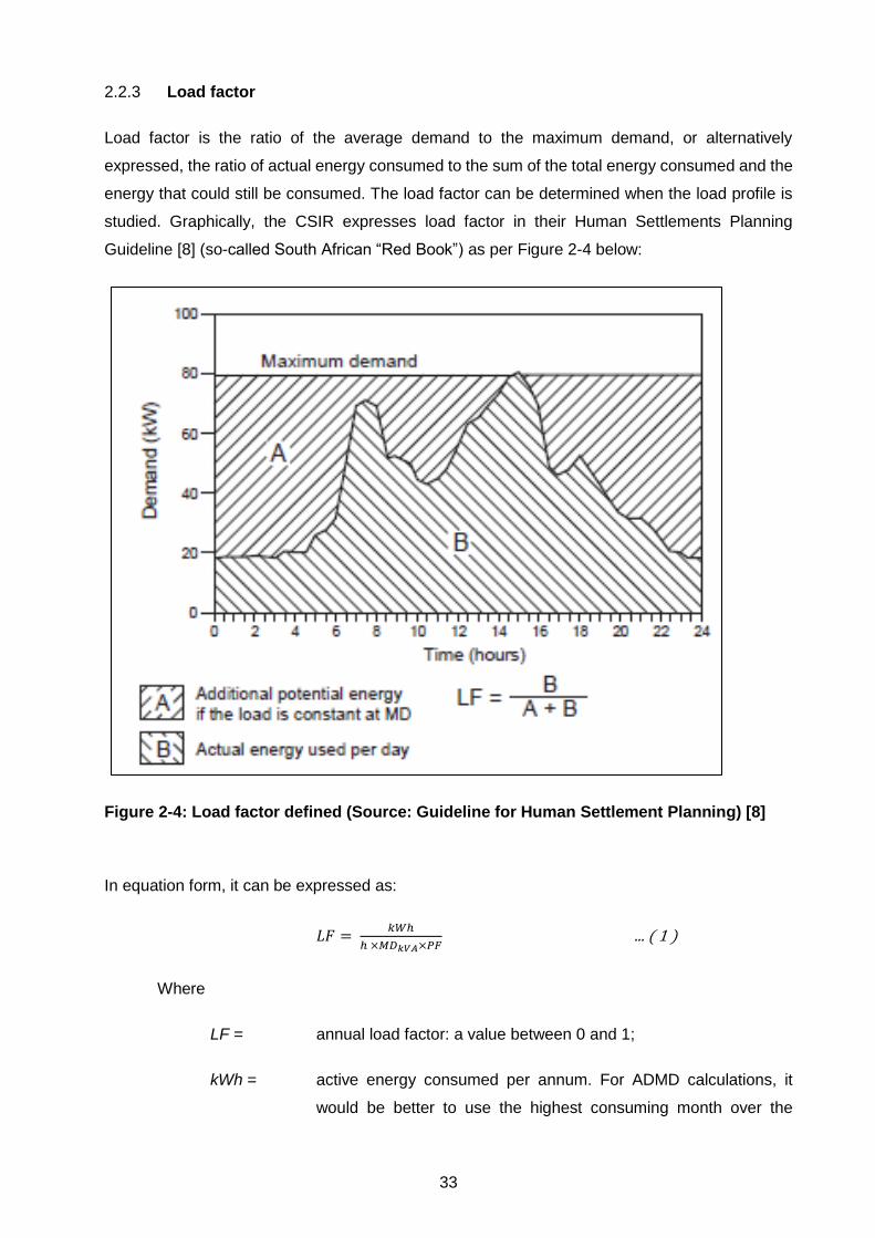
2.2.3 Load factor
Load factor is the ratio of the average demand to the maximum demand, or alternatively
expressed, the ratio of actual energy consumed to the sum of the total energy consumed and the
energy that could still be consumed. The load factor can be determined when the load profile is
studied. Graphically, the CSIR expresses load factor in their Human Settlements Planning
Guideline [8] (so-called South African “Red Book”) as per Figure 2-4 below:
Figure 2-4: Load factor defined (Source: Guideline for Human Settlement Planning) [8]
In equation form, it can be expressed as:
𝐿𝐹 = 𝑘𝑊ℎ
ℎ ×𝑀𝐷𝑘𝑉𝐴×𝑃𝐹 ... ( 1 )
Where
LF = annual load factor: a value between 0 and 1;
kWh = active energy consumed per annum. For ADMD calculations, it
would be better to use the highest consuming month over the

34
design lifespan of the load under consideration and to reduce the
hours accordingly;
h = hours per month;
MDkVA = Maximum demand in kVA;
PF = Power factor, a value between 0 and 1. For residential purposes
this can be assumed to be > 0.95, provided that the load has not
become too inductive. Residential load historically is assumed to be
near unity power factor, but the use of compact fluorescent lamps,
switch mode power supplies, heat pumps and air-conditioners will
change residential load from resistive to inductive.
By assuming a load factor, the maximum demand can be calculated if the energy consumption is
known, and the energy consumption can be calculated if the maximum demand is known. As this
dissertation shows, the maximum demand is a very important design parameter and it is important
to understand the factors that are used to calculate it or that have an effect on it.
The CSIR’s Human Settlements Planning and Design Guideline [8] indicates that the load factor
for high consumption load classes could be changed by demand side management techniques,
such as ripple control to control hot water or other non-essential loads.
A study by Mistry and Roy [9] indicates that the load factor grows as load grows. This implies that
energy consumption grows faster than maximum demand.
2.2.4 ADMD
The previous section mentioned the importance of the maximum demand. When the maximum
demand of a network is related to the maximum demand per consumer, the after diversity
maximum demand (ADMD) is calculated. This dissertation furthermore shows that the ADMD is
one of the key parameters that is central to long-term load forecasting and network design.
The CSIR’s Guidelines for Human Settlement Planning and Design [8] and Eskom [10] defined
ADMD as the average maximum demand of a simultaneous group of consumers. Per definition,
the equation for ADMD may be written as:
𝐴𝐷𝑀𝐷(𝑛) = 𝑀𝐷(𝑛)
𝑛 ... ( 2 )
Where

35
ADMD(n) = ADMD for n customers
MD(n) = Maximum demand for n customers
n = Number of consumers
A study by McQueen et al [11] refers to the related formulae used in the electricity industry for
determining the demand of a group of consumers as Prevalent Engineering Practice (PEP), and
states the origins of these formulae as the work of JG Boggis, published in 1953. Boggis [12]
states these PEP formulae in principle as follows:
𝑀𝐷 = 𝑛 ×𝐷𝐹 ×𝐴𝐷𝑀𝐷 ... ( 3 )
𝐴𝐷𝑀𝐷 = lim𝑛→∞
1
𝑛∑ 𝑀𝐷𝑖𝑛𝑖=0 ... ( 4 )
𝐷𝐹 = 1 + 𝑘
𝑛 ... ( 5 )
Where
ADMD = After Diversity Maximum Demand
MD = Maximum demand, usually over a year
MDi = Maximum demand of ith consumer
n = Number of similar consumers
DF = Diversity factor
k = Coincidence factor
It is interesting to note the slight variance in the approach to the ADMD calculation when
considering equations 2 and 4.
The literature studied contained variances in the number of consumers for which the ADMD
stabilized. While McQueen [11] and Boggis [12] use the definition that the ADMD is accurate for
a very large group (i.e. close to infinity), the Human Settlement Planning Guideline [8] and Eskom
[10] generally accept that the ADMD for residential consumers is constant for a 1000 or more
consumers. Boggis does state that 100 households are a large enough group. Prior to the work
of Boggis, Bary [13] also indicated through studies conducted in the late 1930s and early 1940s
that a group of 100 similar load-class consumers are sufficient, and even observed that groups

36
as small as 30 to 50 consumers are sufficient to conclude an ADMD value that would not vary
much when the number of consumers increases. Gaunt et al [14] observe that beyond
approximately 150 consumers, the ADMD does not change.
In the author’s experience, a group of 100 consumers is a conveniently sized group. One hundred
consumers can still conveniently be connected to a 500 kVA transformer. One thousand
consumers dictate that the ADMD applies to MV feeder or substation level, but should not differ
much from the ADMD of a 100 or 150 consumers.
Generally, the ADMD increases as the number of consumers decreases due to a lack of diversity.
Apart from the formulae above, ADMD can otherwise be determined through direct measurement,
the energy load factor method or through appliance modelling. A discussion of each method
follows.
Direct measurement
Direct measurement is perhaps the best method, but the maturity of the network and any non-
residential loads must be known, as the non-residential loads should be deducted to obtain the
residential portion. The CSIR’s Guidelines for Human Settlement Planning and Design [8]
provides the formula for determining domestic maximum demand when non-domestic load is also
present:
𝑀𝐷𝑟𝑒𝑠𝑖𝑑𝑒𝑛𝑡𝑖𝑎𝑙 = 𝑀𝐷𝑡𝑜𝑡𝑎𝑙 − 𝑀𝐷𝑛𝑜𝑛−𝑟𝑒𝑠𝑖𝑑𝑒𝑛𝑡𝑖𝑎𝑙 ... ( 6 )
Where
MD = Maximum demand
This formula is flawed due to diversity between load classes (refer to figure 2-3). The formula is
only valid if the domestic and non-domestic loads have coinciding maximum demands, meaning
the maximum demands must take place at the same time. Vectorial subtraction should take place,
meaning a 18:00 non-domestic load value must be subtracted from the 18:00 total demand value
to yield a 18:00 non-domestic value.
Care should also be taken when measurements are used. The sampling period plays a major
role. Own calculations from one-minute load profiles indicate that there is a margin of error as the
sampling period of measurements is increased. This margin is even larger when load control is
present.

37
Figure 2-5: Measurement error of the maximum demand of a 10 MVA network, expressed
as a percentage, as a result of integration over time compared to one-minute
measurements for (a) seven consecutive days and (b) one month
0.0%
5.0%
10.0%
15.0%
20.0%
25.0%
30.0%
35.0%
40.0%
0 10 20 30 40 50 60 70
Mea
sure
men
t er
ror
(%)
Integration period (minutes)
Measurement error of maximum demand per day for an arbitrary week of a typical 10 MVA network
% error: 2013-05-01 % error: 2013-05-02 % error: 2013-05-03
% error: 2013-05-04 % error: 2013-05-05 % error: 2013-05-06
% error: 2013-05-07
0.0%
5.0%
10.0%
15.0%
20.0%
25.0%
30.0%
35.0%
40.0%
0 10 20 30 40 50 60 70
Mea
sure
men
t er
ror
(%)
Integration period (minutes)
Measurement error of maximum demand per day for a complete month for a 10MVA network
% error: 2013-05-01 % error: 2013-05-02 % error: 2013-05-03 % error: 2013-05-04% error: 2013-05-05 % error: 2013-05-06 % error: 2013-05-07 % error: 2013-05-08% error: 2013-05-09 % error: 2013-05-10 % error: 2013-05-11 % error: 2013-05-12% error: 2013-05-13 % error: 2013-05-14 % error: 2013-05-15 % error: 2013-05-16% error: 2013-05-17 % error: 2013-05-18 % error: 2013-05-19 % error: 2013-05-20% error: 2013-05-21 % error: 2013-05-22 % error: 2013-05-23 % error: 2013-05-24% error: 2013-05-25 % error: 2013-05-26 % error: 2013-05-27 % error: 2013-05-28% error: 2013-05-29 % error: 2013-05-30
Measurement errorat 30-minute integration
(a)
(b)
Sundays – no load control

38
The measurement error was calculated by comparing the average value during an integration
period with the maximum integrated one-minute value recorded during the same integration
period.
In Figure 2-5 (a), the 5th May 2013 was a Sunday. Load control was not implemented on the
Sunday, and a smaller measurement error is observed. It is not clear why the Monday (6th May
2013) would calculate much lower errors at 5-minute, 10-minute, 15-minute and 20-minute
integration intervals, as load control was implemented on the 6th May 2013 for the load profiles
studied. When a full month’s data were assessed (refer to Figure 2-5 (b), all the Sundays
displayed the same result, while most days with load control present have increased percentage
errors.
It is interesting to note that a 10% to 15% error is made on 30-minute integration with load control
present. A 30-minute integration period is used for billing purposes in South Africa. When load
control is not implemented, the measurement error will only be approximately 3%.
Therefore, when using measurement values, especially when load control is implemented, the
ADMD will be calculated 10% to 15% lower than what it should be when it is based on 30-minute
integration. In other words, if a network is designed according to the ADMD calculated from this
set of measurement data, the cables and transformers will see a higher load than what the
network will be designed for.
Alberts and De Kock [1] illustrated that load control increased the selected network’s maximum
demand by 11%. The calculation in Figure 2-5 is based on the same network’s load profiles used
by Alberts and De Kock to illustrate the effect of load control on the maximum demand (refer to
Figure 2-13). The compounded effect of load control and the measurement error over a 30-minute
integration period is in the range 21-25% (10 to 15% for measurement error plus 11% for load
control impact on maximum demand). This example clearly illustrates the impact load control has
on ADMD.
Energy load factor method
The energy load factor method uses measured or estimated kWh sales per month and an
estimated load factor to calculate the ADMD. Rewriting Equation 1 for load factor to solve for the
maximum demand, the formula becomes:

39
𝑀𝐷𝑘𝑉𝐴 = 𝑘𝑊ℎ
ℎ ×𝐿𝐹×𝑃𝐹 ... ( 7 )
Load factor per day, per month and per annum will differ due to the weekly cycle of load profiles
and the seasonal changes during the year. In South Africa, the weekend domestic load profile is
generally lower than the weekday profile. In Ghana, the weekend domestic load profile tends to
be the same or slightly higher than weekday profiles on MV feeders with a predominant residential
component (refer to Figure 1-1).
Appliance modelling
Appliance modelling is used to model the contribution of appliances during peak period, which
would make up the maximum demand. However, the Human Settlement Planning guideline [8]
warns that for high and very high-income groups, this method tends to underestimate the demand.
Appliance modelling techniques are most suitable to investigate the effects on load factor and
ADMD when an appliance is changed, for example replacing electrical geysers with solar geysers.
2.2.5 Demand factor, coincidence and diversity
Beaty and Fink [15] in the Standard Handbook for Electrical Engineers define the demand factor,
coincidence and diversity factor, and these definitions can be expressed in formula format as
follows:
𝐷𝑒𝑚𝑎𝑛𝑑 𝑓𝑎𝑐𝑡𝑜𝑟 = 𝑀𝑎𝑥𝑖𝑚𝑢𝑚 𝑑𝑒𝑚𝑎𝑛𝑑
𝑇𝑜𝑡𝑎𝑙 𝑐𝑜𝑛𝑛𝑒𝑐𝑡𝑒𝑑 𝑙𝑜𝑎𝑑 ... ( 8 )
𝐶𝑜𝑖𝑛𝑐𝑖𝑑𝑒𝑛𝑐𝑒 = 𝑀𝑎𝑥𝑖𝑚𝑢𝑚 𝑑𝑒𝑚𝑎𝑛𝑑
∑𝑆𝑦𝑠𝑡𝑒𝑚 𝑐𝑜𝑚𝑝𝑜𝑛𝑒𝑛𝑡 𝑚𝑎𝑥𝑖𝑚𝑢𝑚 𝑑𝑒𝑚𝑎𝑛𝑑 ... ( 9 )
𝐷𝑖𝑣𝑒𝑟𝑠𝑖𝑡𝑦 = 1
𝐶𝑜𝑖𝑛𝑐𝑖𝑑𝑒𝑛𝑐𝑒 ... ( 10 )
The demand factor is expressed as a percentage. It expresses the ratio of maximum demand to
total connected load as a percentage. The value is between 0% and 100%. This value can never
be more than 100% due to the diversity between loads.
Coincidence is expressed as a percentage and can never be more than 100%. Typically, the
coincidence for a group of consumers would be the maximum demand as measured for such a
group of consumers, divided by the sum of the individual consumer maximum demands. The

40
maximum demand will generally be lower than the sum of the maximum demands, since it is
unlikely that consumer maximum demands will coincide on day and time.
Beaty and Fink [15] provide the following table of diversity factors:
Table 2-2: Diversity factors as tabled by the Standard Handbook for Electrical
Engineers, Table 18-26 [15]
Elements of system between which diversity factors are stated
Residential lighting
Commercial lighting
General power
Large users
Per level
Between individual users 2.0 1.46 1.45
Between transformers 1.3 1.3 1.35 1.05
Between feeders 1.15 1.15 1.15 1.05
Between substations 1.1 1.10 1.1 1.1
Between users and a particular point in the network
From users to transformer 2.0 1.46 1.44
From users to feeder 2.6 1.90 1.95 1.15
From users to substation 3.0 2.18 2.24 1.32
From users to generating station 3.29 2.40 2.46 1.45
The diversity factors (or its reciprocal, coincidence) between users and a particular point in the
network from Table 2-2 can be plotted as follows:
Figure 2-6: Diversity factors for a power system (derived from Table 2-2)
It is important to understand that consumer behaviour and the utilization of electricity would differ
from country to country and are dependent on factors such as climate, pricing signals, consumer
0.00.10.20.30.40.50.60.70.80.91.0
1.01.21.41.61.82.02.22.42.62.83.0
fro
m u
sers
to
MV
/LV
tran
sfo
rme
rs
fro
m u
sers
to
MV
fee
der
s
fro
m u
sers
to
HV
.MV
su
bst
atio
n
fro
m u
sers
to
gen
erat
ors
Co
inci
den
ce
Div
ersi
ty
Diveristy and coincidence factors in a power system
Diversity (Beaty & Fink) Coincidence (Beaty & Fink)

41
behaviour and EEDSM policies. Therefore, published factors should be considered against the
background of the environment for which it has been published (in the case of the Standard
Handbook for Electrical Engineers [15]: against conditions prevailing in the United States of
America). They should be adjusted for instance where the climate is different, or where electricity
is used for water heating if published figures excluded for argument sake water heating.
When considering losses, a load would not necessarily contribute its loss measured at maximum
demand to the system peak, since the peaks do not necessarily coincide. This factor is referred
to as the peak responsibility factor.
Eskom recommends the coincidence factors in Table 2-3 in electrification projects for non-
residential load [10].
Table 2-3: Peak contribution of non-domestic loads (Source: Eskom [10], table in par
3.1b)
Type of load Typical peak time coincidence factor
Clinic 0.05 to 0.15
School 0.05 to 0.10
Shop 0.50 to 1.00
Hospital 0.50 to 1.00
This means that a school would contribute 5% to 10% of its peak time load to the system evening
peak. Of course, for a morning peak, this factor is different. A school typically peaks around mid-
morning.
Already in the 1930s, Constantine Bary [13] did research on the coincidence factors applicable to
groups of similar consumers and postulated that the relationship of coincidence to the number of
consumers follows the path of a rectangular hyperbola. According to Gaunt et al [16], Rusck
suggests a more refined formula. When comparing these two formulae, the difference in essence
only lies in the treatment of the number of consumers: Bary used it as is, while Rusck uses the
square of the number of consumers:
Bary: 𝐸𝑛 = 𝐸𝑛∞ + 1−𝐸𝑛∞
𝑁 ... ( 11 )
Rusck: 𝑘 = 𝑘∞ + 1−𝐸𝑛∞
√𝑁 ... ( 12 )
In these formulae, En and k have the same meaning.

42
It is important to understand diversity as it allows the planner or engineer to compensate for
coinciding maximum demands. Should an engineer or planner fail to understand the diversified
nature of loads, it may result in under-designed or over-designed networks.
2.2.6 Unbalance and diversity correction factors
Historically, a few empirical formulae were also used to apply diversity and unbalance correction
factors to voltage drop calculations on feeder designs, as summarized by Gaunt et al [16] and
Eskom [17]. The table below contains the author’s summary of these methods.
Table 2-4: Historical empirical diversity correction and unbalance correction factors
used in South Africa, available with ReticMaster simulation software
Formula Diversity correction Unbalance correction
AMEU [17]
𝐷𝐶𝐹(𝑁) = 1 + 2
𝑁 ... ( 13 )
𝑈𝐶𝐹(𝑁) = 1 + 2.8
√𝑁 ... ( 14 )
DT [17] (Eskom)
𝐷𝐶𝐹(𝑁) = 1 + 8
𝐴𝐷𝑀𝐷 ×𝑁
For ADMD ≤ 5 ... ( 15 )
𝐷𝐶𝐹(𝑁) = 1 + 12
𝐴𝐷𝑀𝐷 ×𝑁
For ADMD > 5 ... ( 16 )
𝑈𝐶𝐹(𝑁) = 1 + 2.8
√𝑁 ... ( 17 )
British [16] 𝐹1×𝐹2 = (1 +4.14
√𝑁)× (1 +
𝑘
𝐴𝐷𝑀𝐷×𝑁) ... ( 18 )
where k=8 or 12
User defined [17]
𝐷𝐶𝐹(𝑁) = 1 + 𝑚 ∙ 𝑁𝑐 ... ( 19 ) m,c = user defined variables
𝑈𝐶𝐹(𝑁) = 1 + 𝑥 ∙ 𝑁𝑦... ( 20 ) x, y = user defined variables
Neutral Not applicable Vector sum
Where DCF(N) = Diversity correction function for N consumers UCF(N) = Unbalance correction function for N consumers
Prior to the inclusion of the Herman-Beta voltage drop calculation method in NRS034, the
preferred method by municipalities in South Africa was the AMEU method for diversity and
unbalance correction. The DT formulae were not widely used and were experimental formulae
developed by Eskom.
Voltage drop in empirical form in a balanced multi-phase system is calculated as:

43
∆𝑉𝑠𝑒𝑐𝑡𝑖𝑜𝑛 = 𝐼𝐴𝐷𝑀𝐷 ×𝑛×𝐷𝐶𝐹(𝑛)×𝑍𝑠𝑒𝑐𝑡𝑖𝑜𝑛 ... ( 21 )
Where
ΔVsection = Volt drop of the line or cable section, in volts
IADMD = ADMD current in ampere for a group of 1000 consumers
n= Number of houses or consumers
DCF (n) = Diversity correction factor as per unbalance and diversity correction
factors
Zsection = Impedance of the line or cable section, in ohms
In a single-phase system, the voltage drop will also be experienced over the neutral conductor
and must be added.
The total voltage drop is the sum of the voltage drop of each of the sections along a feeder. A
section is the section of a line or cable between distribution points. On a line, it would be between
pole-top boxes and on a cable feeder between distribution or metering kiosks.
At present, the Herman-Beta method is used in load flow software such as Reticmaster.
Reticmaster calculates unbalance through vectorial summation.
2.2.7 Relationship between coincidence and load factor
Bary [13] also related coincidence to load factor. His measurements were done prior to and during
World War II in the United States of America during December (American winters) and he found
that the relationship held true during the peace, defence (period leading up to the war) and war
periods.
Bary [13] published his curves in the late 1930s and early to mid-1940s. Bary composed the
following curves from measurements:

44
Figure 2-7: Bary's curve for various measurements of coincidence against load factor
[13]
The Bary curve appeared in an unpublished version of NRS058 [18] as part of the South African
electricity consumption tariff design methodology (unpublished as at date of compiling this
dissertation).
The US Department of Defence [19] declassified a standard that contained a similar graph for
use at its facilities. Although the document is labelled as “cancelled”, it still illustrates how widely
Bary’s work has been adopted.

45
Figure 2-8: Bary coincidence factors related to load factor [18]
The Bary curve is applicable to the conditions that prevailed in the United States of America during
the 1930s and 1940s, so the formulae may not necessarily hold true under different circumstances
(i.e. different control and limiting strategies, appliance design, consumer behaviour, climate
conditions etc.).
At a load factor of 80%, it does confirm the expectation that the coincidence in Ghana for similar
residential consumers is high (±87%). However, the same also holds true for any load factor
between 40% and 70%, which still yields a coincidence factor of 80%.
What is significant of Bary’s work, is that a change in load factor will change the coincidence
factors and vice versa, especially at low load factors (<40%). The Human Settlement Planning
Guideline [8] and Eskom [10] indicate that load factors for domestic load is generally 40% and
less.
A load shift or energy efficiency exercise will change the load profile and the load factor associated
with it. This implies that a change in coincidence factors can be expected.

46
2.2.8 Load loss factor
Technical losses are inherent to any transmission or distribution system due to the energy lost as
a result of the impedance of a network. Technical losses can be empirically calculated (I2R, I2Z,
etc.), or it can be estimated using the load loss factor. The Standard Handbook for Electrical
Engineers [15] defines the load loss factor as follows:
𝐹𝐿 = 𝐴𝑣𝑒𝑟𝑎𝑔𝑒 𝑝𝑜𝑤𝑒𝑟 𝑙𝑜𝑠𝑠 𝑜𝑣𝑒𝑟 𝑝𝑒𝑟𝑖𝑜𝑑 𝑜𝑓 𝑡𝑖𝑚𝑒
𝑀𝑎𝑥𝑖𝑚𝑢𝑚 𝑝𝑜𝑤𝑒𝑟 𝑙𝑜𝑠𝑠 𝑜𝑣𝑒𝑟 𝑝𝑒𝑟𝑖𝑜𝑑 𝑜𝑓 𝑡𝑖𝑚𝑒 ... ( 22 )
Where
FL = Loss factor: a value between 0 and 1. It is also sometimes referred
to as the load factor of losses. The symbol LLF is sometimes used
instead of FL
The loss factor only refers to technical losses and excludes non-technical losses. Non-technical
losses include all losses not due to the impedance of the system, for example theft, billing errors,
CT or VT ratio errors, faulty meters, faulty CTs, faulty VTs, meter reading errors, unmetered load
etc. Beaty and Fink [15] provide the following formula relating the two factors based on studies of
various load profiles:
𝐹𝐿 = 0.15𝐿𝐹 + 0.85𝐿𝐹2 ... ( 23 )
Where
LF = Annual load factor: a value between 0 and 1.
FL = Loss factor: a value between 0 and 1.
Technical losses are usually estimated over a year, for example 8760 hours. The loss factor and
the load factor can be related and the loss factor is usually less than the load factor. Mistry and
Roy [9] report these values to be 0.2 and 0.8 instead of 0.15 and 0.85 respectively.
The cost of losses is determined as follows:
𝐶𝑜𝑠𝑡 𝑜𝑓 𝑙𝑜𝑠𝑠𝑒𝑠 𝑝𝑒𝑟 𝑘𝑊ℎ = 𝐹𝑠𝑃
8760 𝐹𝐿+ 𝐸 ... ( 24 )
Where
FS = Responsibility factor
FL = Loss factor: a value between 0 and 1

47
E = Energy cost (R/kWh)
P = Annual cost of system capacity (R/kW-year)
Should the losses be incorrectly calculated, the life cycle costing would be incorrect. The cost of
losses forms an important part of the evaluation of masterplan alternatives where full life cycle
costs should rather be one of the key considerations as opposed to capital cost only.
2.2.9 Load growth
Load growth is modelled using S-curve behaviour. A typical S-curve formula used by Eskom is
the Gompertz curve [20].
𝑓(𝑥) = 1
1+10𝐶[(2 + 10𝐶) (𝐴 +
(1−𝐴)
1+10𝐶𝑒−7𝑥/𝐵) − 1] . .. ( 25 )
Where
f(x) = Unitized annual peak load estimate in year x, a value between 0
and 1. The value can be multiplied by the future estimated load to
scale it to the correct future load in year x.
A = The base load expressed as a fraction of the future load, between
0 and 1.
B = The number of years until saturation, usually 20, but can be any
positive value. The value is usually an integer.
C = A figure between 1 and 10 indicating the growth rate. 1 means fast
initial growth, while 10 means slow initial growth.
x = The year of calculation.
An example of a growth forecast based on different growth rates is illustrated in Figure 2-9 for a
1000 residential units at a final ADMD of 1.3 kVA per residential unit, 20-year saturation and an
initial load of 50 residential units at 0.7 kVA per unit:
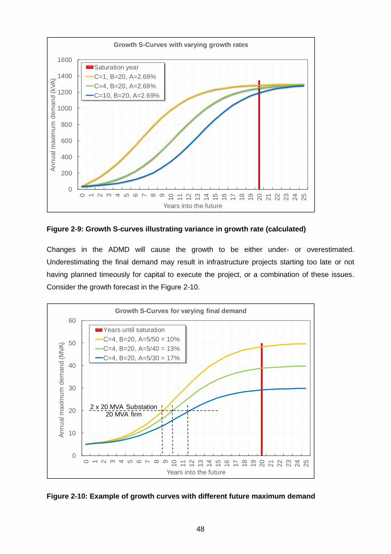
48
Figure 2-9: Growth S-curves illustrating variance in growth rate (calculated)
Changes in the ADMD will cause the growth to be either under- or overestimated.
Underestimating the final demand may result in infrastructure projects starting too late or not
having planned timeously for capital to execute the project, or a combination of these issues.
Consider the growth forecast in the Figure 2-10.
Figure 2-10: Example of growth curves with different future maximum demand
0
200
400
600
800
1000
1200
1400
1600
0 1 2 3 4 5 6 7 8 9
10
11
12
13
14
15
16
17
18
19
20
21
22
23
24
25
An
nu
al m
axi
mu
m d
em
an
d (kVA
)
Years into the future
Growth S-Curves with varying growth rates
Saturation year
C=1, B=20, A=2.69%
C=4, B=20, A=2.69%
C=10, B=20, A=2.69%
0
10
20
30
40
50
60
0 1 2 3 4 5 6 7 8 9
10
11
12
13
14
15
16
17
18
19
20
21
22
23
24
25
An
nu
al m
axi
mu
m d
em
an
d (M
VA
)
Years into the future
Growth S-Curves for varying final demand
Years until saturation
C=4, B=20, A=5/50 = 10%
C=4, B=20, A=5/40 = 13%
C=4, B=20, A=5/30 = 17%
2 x 20 MVA Substation20 MVA firm

49
In Figure 2-10, a 2 x 20 MVA substation operated within firm capacity means that the substation
load must not exceed 20 MVA. When the load exceeds 20 MVA, either a third transformer must
be installed, the existing transformers replaced with larger transformers, or load must be shifted
to another substation. Should a planner have forecasted the load incorrectly by using an
inappropriate ADMD value, typical scenarios may play out as follows:
a) Underestimating the ADMD:
i. Suppose the planner estimated the ADMD to be 3 kVA per residential unit for
10 000 residential units. The planner will reach an ADMD of 30 MVA and will
propose that an upgrade or strengthening project must be completed by year 11.
ii. Suppose, however, that the planner missed critical information and the ADMD
should have been calculated as 5 kVA per unit. In such a case the strengthening
project for the substation should have been implemented by year 9. The project
may have started two years too late.
b) Overestimation of the ADMD:
i. If, for instance, the correct future forecast was 30 MVA, but the planner initially
predicted it to be 50 MVA, the two 20 MVA transformers would have been replaced
by three 40 MVA transformers by year 9, but the future load of 30 MVA is less than
a third of the newly installed capacity of 120 MVA (80 MVA firm).
ii. The substation will consume no-load losses on two spare transformers and would
have laid out unnecessary capital, which may be subjected to interest payments
over a 20-year period for a loan.
iii. Additional insurance costs for unnecessary equipment will also be paid.
iv. Due to the long lead times on transformers, the decision to procure the
transformers would have been taken up to 24 months earlier - too late to stop the
process if it is later discovered to have been an error.
As is illustrated in the example above, it is important to understand load growth techniques, as it
enables an engineer or planner to determine the future load of a network. Knowing the future load
allows for the sizing of equipment. Again, maximum demand is the important factor calculated
through this method. The base load (i.e. in year 0) affects the position along the S-curve for the
present moment in time. If the base load is very low, the position is closer to the start of the S-
curve. If a development is 75% developed, the position is closer to the saturation point.
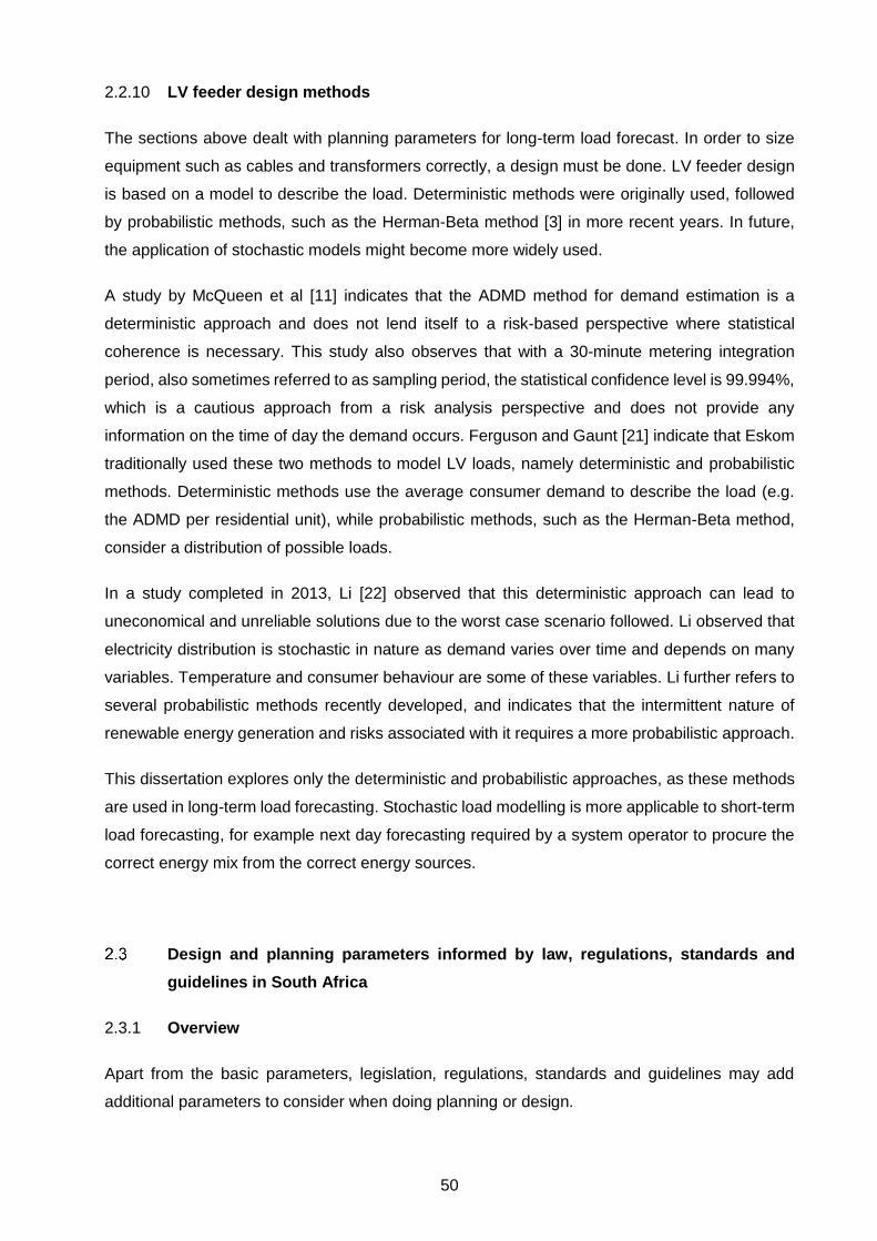
50
2.2.10 LV feeder design methods
The sections above dealt with planning parameters for long-term load forecast. In order to size
equipment such as cables and transformers correctly, a design must be done. LV feeder design
is based on a model to describe the load. Deterministic methods were originally used, followed
by probabilistic methods, such as the Herman-Beta method [3] in more recent years. In future,
the application of stochastic models might become more widely used.
A study by McQueen et al [11] indicates that the ADMD method for demand estimation is a
deterministic approach and does not lend itself to a risk-based perspective where statistical
coherence is necessary. This study also observes that with a 30-minute metering integration
period, also sometimes referred to as sampling period, the statistical confidence level is 99.994%,
which is a cautious approach from a risk analysis perspective and does not provide any
information on the time of day the demand occurs. Ferguson and Gaunt [21] indicate that Eskom
traditionally used these two methods to model LV loads, namely deterministic and probabilistic
methods. Deterministic methods use the average consumer demand to describe the load (e.g.
the ADMD per residential unit), while probabilistic methods, such as the Herman-Beta method,
consider a distribution of possible loads.
In a study completed in 2013, Li [22] observed that this deterministic approach can lead to
uneconomical and unreliable solutions due to the worst case scenario followed. Li observed that
electricity distribution is stochastic in nature as demand varies over time and depends on many
variables. Temperature and consumer behaviour are some of these variables. Li further refers to
several probabilistic methods recently developed, and indicates that the intermittent nature of
renewable energy generation and risks associated with it requires a more probabilistic approach.
This dissertation explores only the deterministic and probabilistic approaches, as these methods
are used in long-term load forecasting. Stochastic load modelling is more applicable to short-term
load forecasting, for example next day forecasting required by a system operator to procure the
correct energy mix from the correct energy sources.
Design and planning parameters informed by law, regulations, standards and
guidelines in South Africa
2.3.1 Overview
Apart from the basic parameters, legislation, regulations, standards and guidelines may add
additional parameters to consider when doing planning or design.

51
The following documents govern compliance with technical and supply quality performance
requirements in South Africa in the electricity supply industry:
• South African Grid Code (consisting of multiple sub-codes);
• NRS specifications and SANS standards, and
• Guidelines for Human Settlement Planning [8].
These documents are briefly discussed in the following paragraphs:
2.3.2 Grid code
The South African Grid Code (SAGC) [23] is a collection of smaller codes. The Grid Code is the
result of a legal requirement in the Electricity Regulation Act, Act 4 of 2006. This Act determines
that the National Energy Regulator of South Africa (NERSA) should determine rules for
compliance by licensees.
Table 2-5: South African Grid Code components
Grid Code document Basic contents / Scope
Transmission system – Version 8, July 2010
Grid Code Preamble Sets out context of Grid code Definition of terms used in Grid Code
Governance Code Provisions necessary for overall administration of the Grid Code
Network Code Connection conditions for generators, distributors and end-use customers Standards for the transmission system
System Operation Code Responsibilities and roles for operation, maintenance and outage planning
Metering Code Transmission tariff and energy trading metering requirements Responsibility for metering installations
Transmission Tariff Code Objectives of transmission service pricing
Information Exchange Code Requirements for exchange of planning, operational and maintenance information
Renewable Power Plant, Version 2.8, November 2012
Grid Connection Code for Renewable Power Plants
Minimum technical and design requirements for grid connection of renewable power plants
Distribution system, Version 6, July 2014
Distribution Code Glossary and Definitions
Definitions applicable to Distribution Code
Distribution Code - Network Code
Set basic rules of connecting to the distribution system. Specify technical requirements to ensure safety and reliability
Distribution Code - System Operating Code
Sets out responsibilities and roles for operation of distribution system
Distribution Code - Tariff Code
Sets out objectives for pricing and tariff structures

52
Grid Code document Basic contents / Scope
Distribution Code - Metering Code
Compliance requirements for tariff and energy trading metering, responsibilities for metering installations Appropriate procedures for maintenance, testing, collection, validation and verification of metering data
Distribution Code - Information Exchange Code
Requirements for exchange of planning, operational and maintenance information
The following criteria are extracted to emphasize the factors that can be altered through the
application of distributed generation (DG) (e.g. voltages may rise above limits set by the Grid
Code).
The Transmission Network Code [23] requires that load forecasts be done every year for the ten
years ahead and that load forecasts of end-users and distributors be obtained. It states that
diversity factors as measured or calculated may be applied to the data to provide sufficient
planning information at higher levels. Therefore, it is important to ensure that selected diversity
factors are not adversely influenced by for instance the roll-out of solar PV systems.
The Transmission Network Code further defines the minimum and maximum voltages to which
systems must comply, the target voltages when performing planning actions, power factor,
protection requirements, fault level management obligations, reliability and contingency planning
requirements. The minimum and maximum voltages will perhaps always remain the main criteria
for design compliance.
Power factor limits are stated and rules for engagement with stakeholders when fault level
variations take place, are provided. Power quality and protection requirements are provided.
These are all important aspects when considering the implementation of DG.
The Transmission Tariff Code [24] provides a section on loss charges through the application of
loss factors. When loss factors change, the underlying basis of a tariff design may be influenced.
The South African Distribution Code (SADC) [25] is a part of the SAGC and applies to all
distributors. As for the Transmission Network Code, the important parameters governed by the
SADC Network Code is voltage and power factor and it states further that fault levels as agreed
through contracts must not be exceeded. Adding DG has the potential to raise fault levels above
contractual limits.
The Grid Connection Code for Renewable Power Plants [26] supplements the Transmission and
Distribution Network Codes and provides the compliance requirements of Renewable Power
Plants (RPPs). This section of the Grid Code provides criteria for operation and control of

53
renewable power plants. These criteria are provided to protect the grid and to ensure proper
quality of supply.
Unregistered solar PV systems are already installed and the present effects of excess energy
injected into the grid are most likely negligible or overlooked due to the isolated occurrence
thereof. However, as the tariff or pricing signals change and the risk of unavailable electricity to
the general user increases, the occurrence of solar rooftop PV is expected to increase. These
effects may cause unwanted performance of the grid as the system operators are unaware of it,
and have not tested or simulated the effects of connection or disconnection.
2.3.3 Standards and specifications overview
The South African Bureau of Standards (SABS) regulates all the standards for compliance in the
electricity supply industry. Most standards are IEC standards, which are adopted as SANS
standards, while Rationalized User Specifications (NRS) guide further specific requirements. The
most notable standards and specifications are:
• NRS 048: Quality of supply
• SANS 507 / NRS 034: Guidelines for the provision of electrical distribution networks in
residential areas
• SANS 10142: The wiring code of premises
2.3.4 NRS 048: Quality of supply
NRS 048, especially Part 2, deals with the quality of supply voltage and frequency requirements
for electricity networks in South Africa. NRS 048 is also referenced by the Grid Code and the
criteria highlighted for the Grid Code are not repeated here again.
2.3.5 SANS 507 / NRS 034
NRS 034 [3] defines the network voltage drop calculation methodology in use at present in South
Africa for low voltage installations through application of the Herman-Beta voltage drop method.
This method uses a beta distribution curve with α and β parameters, an ADMD (kVA / household)
and the limiting circuit breaker current rating (defined by the symbol c). ADMD can be related to
the mean and standard deviation of a Beta distribution curve. The Beta distribution curve was
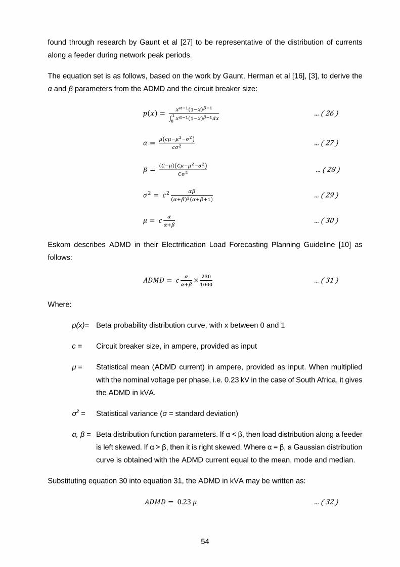
54
found through research by Gaunt et al [27] to be representative of the distribution of currents
along a feeder during network peak periods.
The equation set is as follows, based on the work by Gaunt, Herman et al [16], [3], to derive the
α and β parameters from the ADMD and the circuit breaker size:
𝑝(𝑥) = 𝑥𝛼−1(1−𝑥)𝛽−1
∫ 𝑥𝛼−1(1−𝑥)𝛽−1𝑑𝑥1
0
... ( 26 )
𝛼 = 𝜇(𝑐𝜇−𝜇2−𝜎2)
𝑐𝜎2 ... ( 27 )
𝛽 = (𝐶−𝜇)(𝐶𝜇−𝜇2−𝜎2)
𝐶𝜎2 ... ( 28 )
𝜎2 = 𝑐2𝛼𝛽
(𝛼+𝛽)2(𝛼+𝛽+1) ... ( 29 )
𝜇 = 𝑐𝛼
𝛼+𝛽 ... ( 30 )
Eskom describes ADMD in their Electrification Load Forecasting Planning Guideline [10] as
follows:
𝐴𝐷𝑀𝐷 = 𝑐𝛼
𝛼+𝛽×230
1000 ... ( 31 )
Where:
p(x)= Beta probability distribution curve, with x between 0 and 1
c = Circuit breaker size, in ampere, provided as input
μ = Statistical mean (ADMD current) in ampere, provided as input. When multiplied
with the nominal voltage per phase, i.e. 0.23 kV in the case of South Africa, it gives
the ADMD in kVA.
σ2 = Statistical variance (σ = standard deviation)
α, β = Beta distribution function parameters. If α < β, then load distribution along a feeder
is left skewed. If α > β, then it is right skewed. Where α = β, a Gaussian distribution
curve is obtained with the ADMD current equal to the mean, mode and median.
Substituting equation 30 into equation 31, the ADMD in kVA may be written as:
𝐴𝐷𝑀𝐷 = 0.23 𝜇 ... ( 32 )
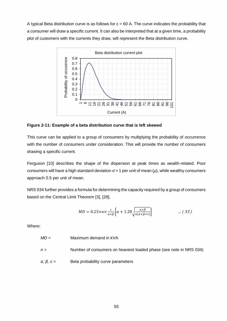
55
A typical Beta distribution curve is as follows for c = 60 A. The curve indicates the probability that
a consumer will draw a specific current. It can also be interpreted that at a given time, a probability
plot of customers with the currents they draw, will represent the Beta distribution curve.
Figure 2-11: Example of a beta distribution curve that is left skewed
This curve can be applied to a group of consumers by multiplying the probability of occurrence
with the number of consumers under consideration. This will provide the number of consumers
drawing a specific current.
Ferguson [10] describes the shape of the dispersion at peak times as wealth-related. Poor
consumers will have a high standard deviation σ > 1 per unit of mean (μ), while wealthy consumers
approach 0.5 per unit of mean.
NRS 034 further provides a formula for determining the capacity required by a group of consumers
based on the Central Limit Theorem [3], [28].
𝑀𝐷 = 0.23×𝑛×𝑐
𝛼+𝛽[𝛼 + 1.28√
𝛼×𝛽
𝑛(𝛼+𝛽+1)] ... ( 33 )
Where:
MD = Maximum demand in kVA
n = Number of consumers on heaviest loaded phase (see note in NRS 034)
α, β, c = Beta probability curve parameters
0
0.1
0.2
0.3
0.4
0.5
0.6
0.7
0.8
1 6
11
16
21
26
31
36
41
46
51
56
61
66
71
76
81
86
91
96
10
1
Pro
babili
ty o
f occure
nce
Current (A)
Beta distribution current plot

56
Equation 33 includes a 10% risk (90% confidence level), represented by the value 1.28 for an
infinite number of degrees of freedom, calculated using published tables for Student’s5 t-
distribution [28]. For different values of confidence, a different value must be selected, e.g. a 95%
confidence level will result in the 1.28 being replaced by 1.65.
Although this formula compensates for lack of diversity for a reduced number of consumers, NRS
034 cautions that this formula is generally not suitable for fewer than 10 consumers per phase.
NRS 034 [3] recommends the following values for the Herman-Beta voltage drop method:
Table 2-6: NRS 034-recommended Herman-Beta parameters for various income
classes for residential load estimation – 15-year forecast values [3]
Consumer class Living Standard Measure
α β c
(A)
ADMD
(kVA)
Rural settlement LSM1 0.35 2.88 20 0.50
Rural village LSM1&2 0.48 2.13 20 0.84
Informal settlement LSM3&4 0.91 8.80 60 1.30
Township area LSM5&6 1.22 5.86 60 2.37
Urban residential I LSM7 1.25 3.55 60 3.59
Urban residential II LSM7&8 1.42 4.10 80 4.72
Urban township complex LSM8 1.42 4.13 80 4.70
Urban multi-storey estate LSM 8 1.37 3.39 80 5.30
NRS 034 indicates that these parameters are for the interior of South Africa. Where cold wet
winters are found, as in the case of the Western Cape, ADMDs are approximately 12% higher.
For coastal areas similar to the climate of Durban, the ADMD can be 12% lower. With a different
ADMD or circuit breaker size, the α and β values will be different.
5 Student was the pseudonym for William Sealy Gosset (1876–1937)

57
2.3.6 NRS 097
NRS 097-2-1 [29] mainly focuses on small scale embedded generation within a utility and
attempts to regulate the connection of small scale embedded generation to the distribution
network. Small scale is defined as smaller than 100 kW and is connected at the LV level. The
document does not have the status of a national standard. It mainly describes metering
arrangements, earthing and synchronization requirements. It does not provide any further
information applicable to this study.
NRS097-2-3 [30] sets simplified connection criteria for low voltage connected generators for
households with a Living Standard Measure (LSM) larger than 7. These criteria attempt to limit
the amount of PV that a utility should allow on feeders (refer to Figure 2-12).
Figure 2-12: NRS097 proposed limits of embedded generation (based on values
contained in [30])
General NRS 097 requirements are:
• Generally, generator sizes should be limited to less than 350 kVA.
• The LV fault level of the customer must be larger than 210 A.
• The total DG that is supplied by a MV feeder should be restricted to 15% of the feeder’s
peak load.
• The total DG connected to a MV/LV transformer should not exceed 75% of the transformer
rating.
For shared LV feeders, the requirements are:
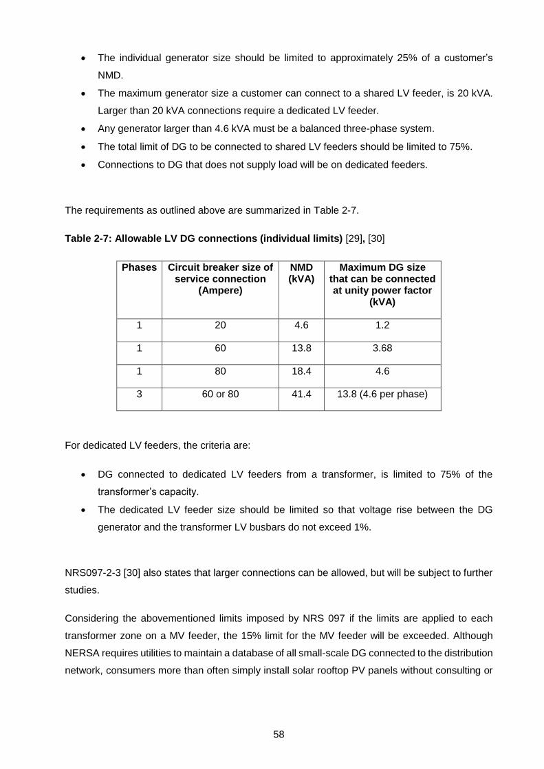
58
• The individual generator size should be limited to approximately 25% of a customer’s
NMD.
• The maximum generator size a customer can connect to a shared LV feeder, is 20 kVA.
Larger than 20 kVA connections require a dedicated LV feeder.
• Any generator larger than 4.6 kVA must be a balanced three-phase system.
• The total limit of DG to be connected to shared LV feeders should be limited to 75%.
• Connections to DG that does not supply load will be on dedicated feeders.
The requirements as outlined above are summarized in Table 2-7.
Table 2-7: Allowable LV DG connections (individual limits) [29], [30]
Phases Circuit breaker size of service connection
(Ampere)
NMD (kVA)
Maximum DG size that can be connected at unity power factor
(kVA)
1 20 4.6 1.2
1 60 13.8 3.68
1 80 18.4 4.6
3 60 or 80 41.4 13.8 (4.6 per phase)
For dedicated LV feeders, the criteria are:
• DG connected to dedicated LV feeders from a transformer, is limited to 75% of the
transformer’s capacity.
• The dedicated LV feeder size should be limited so that voltage rise between the DG
generator and the transformer LV busbars do not exceed 1%.
NRS097-2-3 [30] also states that larger connections can be allowed, but will be subject to further
studies.
Considering the abovementioned limits imposed by NRS 097 if the limits are applied to each
transformer zone on a MV feeder, the 15% limit for the MV feeder will be exceeded. Although
NERSA requires utilities to maintain a database of all small-scale DG connected to the distribution
network, consumers more than often simply install solar rooftop PV panels without consulting or

59
informing the utility. This aspect was investigated by means of simulations to indicate what impact
may be experienced, and is discussed in Chapters 3, 4 and 5.
2.3.7 SANS 10142
SANS 10142 consists of two parts: Part 1, covering the low voltage networks on premises, and
Part 2, covering the medium voltage networks on premises. A Part 3 is envisaged, which will
regulate DC distribution. DC distribution is used typically with solar PV plants between the PV
panels and the inverters. At the time of preparing this dissertation, it had not been published.
SANS 10142-1 [31] defines mostly the requirements for the low voltage wiring of a premises.
Diversity factors for groups of consumers on premises are provided over and above the technical
requirements for design and wiring of electrical reticulation on premises, such as a block of flats
or a cluster housing development (refer to Table 2-8).
Table 2-8: SANS 10142-1 Coincidence factors for residential units [31]
Units per phase
Coincidence factor
Units per phase
Coincidence factor
1 1.00 9 0.46 2 0.72 10 0.45 3 0.62 15 0.42 4 0.57 20 0.40 5 0.53 30 0.38 6 0.50 40 0.37 7 0.48 50 0.36 8 0.47 100 0.34
In SANS 10142, these factors are incorrectly referred to as diversity factors. Coincidence is
smaller than 1, while diversity factors are larger than 1.
SANS 10142 also describes a method for neutral current unbalance calculation, and provides
multiplication factors for use when calculating voltage drop. The formula for voltage drop
published in SANS10142-1 is:
𝑉𝑑 = 𝐹𝑣×𝐼×(𝑅 cos𝜃+𝑋 sin𝜃)𝑥 𝐿
1000 ... ( 34 )
Where
Vd = Voltage drop, in volts
Fv = Multiplication factor for unbalance correction (see table 2-9)

60
I = Current, in amperes
L = Length of conductor / cable, in metres
R = Resistance of conductor, in ohms per kilometre
X = Reactance of conductor, in ohms per kilometre
θ = The phase angle of the load (power factor = cos θ)
Table 2-9: Neutral unbalance multiplication factors for calculating volt drop (refer to [31]
Table E3)
Type of supply and mode of connection Multiplication factor Fv
Direct current load across two conductors 2
Single-phase load between phase and neutral 2
Single-phase load between two phases only 2
Balanced three-phase load on all three phases, neutral unconnected 1
Three identical single-phase loads, one between each phase and connected neutral
1
Unbalanced loads between all three phases and connected neutral:
a) Unbalanced < 75% 1
b) Unbalanced > 75% 2
Unbalanced loads between all three phases and unconnected neutral:
a) Unbalanced < 75% 1
b) Unbalanced > 75% 1.2
2.3.8 Planning Guidelines - overview
Distribution Network Planning in South Africa is guided by the following documents:
• Guideline for Human Settlement Planning, volume II [8]
• DGL 34-431 Eskom Methodology for Network Master Plans and Network
Development Plans [2]
• DGL 34-1284 Geo-based Load Forecast Guideline [20]
• DGL 34-450 Network Planning Reliability Guideline [32]
Although the Reliability Planning Guideline contains critical information when compiling master
plans, it does not contain planning parameters applicable to this study and will not be discussed
further.
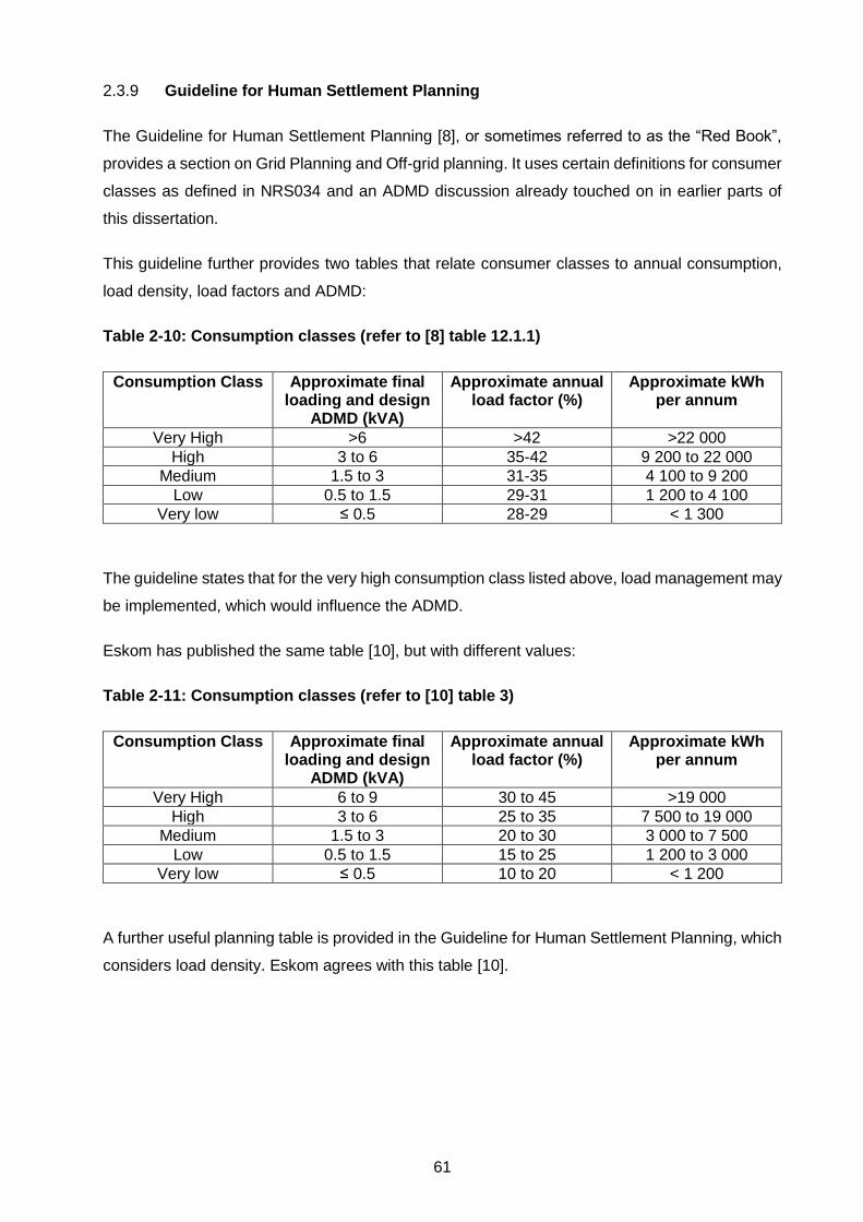
61
2.3.9 Guideline for Human Settlement Planning
The Guideline for Human Settlement Planning [8], or sometimes referred to as the “Red Book”,
provides a section on Grid Planning and Off-grid planning. It uses certain definitions for consumer
classes as defined in NRS034 and an ADMD discussion already touched on in earlier parts of
this dissertation.
This guideline further provides two tables that relate consumer classes to annual consumption,
load density, load factors and ADMD:
Table 2-10: Consumption classes (refer to [8] table 12.1.1)
Consumption Class Approximate final loading and design
ADMD (kVA)
Approximate annual load factor (%)
Approximate kWh per annum
Very High >6 >42 >22 000
High 3 to 6 35-42 9 200 to 22 000
Medium 1.5 to 3 31-35 4 100 to 9 200
Low 0.5 to 1.5 29-31 1 200 to 4 100
Very low ≤ 0.5 28-29 < 1 300
The guideline states that for the very high consumption class listed above, load management may
be implemented, which would influence the ADMD.
Eskom has published the same table [10], but with different values:
Table 2-11: Consumption classes (refer to [10] table 3)
Consumption Class Approximate final loading and design
ADMD (kVA)
Approximate annual load factor (%)
Approximate kWh per annum
Very High 6 to 9 30 to 45 >19 000
High 3 to 6 25 to 35 7 500 to 19 000
Medium 1.5 to 3 20 to 30 3 000 to 7 500
Low 0.5 to 1.5 15 to 25 1 200 to 3 000
Very low ≤ 0.5 10 to 20 < 1 200
A further useful planning table is provided in the Guideline for Human Settlement Planning, which
considers load density. Eskom agrees with this table [10].

62
Table 2-12: Domestic density classification ([8] table 12.1.2, [10] table 4)
Domestic density classification
Stand size (m2) Average load density (kW / km2)
Urban 0.5 ≤ ADMD ≤ 4.5
High density < 1000 400 to 30 000
Medium density 1 000 to 4 000 300 to 5 000
Low density 4 000 to 20 000 100 to 1 500
Rural > 20 000 0.5 to 250
2.3.10 Parameters for non-domestic load
SANS 204 [33] details energy efficiency requirements in non-domestic buildings and lists
maximum demand and energy per annum. Below are average demand values (maximum per
month summed over 12 months, divided by 12).
Table 2-13: Maximum energy demand per building classification for each climatic zone
([33] table 1)
It must be noted that the maximum demand stated above is an annual average maximum
demand, and not the maximum to be expected in the year.
SANS 204 also lists the target energy consumption per m2 per year, as per the table below, with
a footnote that any fossil-fuel non-electrical consumption should be converted to an electrical
equivalent. This statement implies that any energy generated by another energy source will
potentially distort the load factor calculation if not accounted for.

63
Table 2-14: Maximum annual consumption per building classification for each climatic
zone in South Africa ([33] Table 2
SANS 204 annual demand values are achievable with enough effort (and the client’s budget) and
incorporated into the design. However, the energy consumption targets are difficult to achieve.
2.3.11 DGL 34-431 Eskom Methodology for Network Master Plans and Network
Development Plans
Following on the earlier introduction in Paragraph 2.1, the Eskom methodology for Network
Master Plans and Network Development Plans [2] also describes the demand forecast and growth
calculation processes.
The saturation demand forecast and the growth rate are key components of the Eskom planning
process and define how much capacity will eventually be required. The saturation demand is
derived by considering various load classes and their respective load profiles at a lower level.
Since load growth is not uniform across a planning area, the load forecast is further derived
through a geographic approach. The Geographic Load Forecasting (GLF) method employed by
Eskom is discussed in the next section.
The process makes use of ADMD values and load profile shapes per load class at the lowest
level chosen by the planner. Usually, the lowest planning level is selected as MV feeder level, as
MV feeder load readings as a base are available, but it can be taken as low as erven level. An
MV feeder is still made up of the composite load of various load classes. It is critical to understand
that appropriate ADMD values must be applied to the load profile shapes. The ADMD of a

64
residential area for instance is much lower at MV feeder level than at LV feeder or distribution
transformer (MV/LV transformer) level. No diversity values are explicitly stated or used as input
parameters by the GLF tool, as loads are mathematically and geographically summated using the
base values provided from MV feeder level to substation level to HV feeder level to Main
Transmission Substation (MTS) level, assuming that the MV feeder was the lowest level used.
GLF makes provision for a scaling factor, which can be applied to adjust for diversity between
hierarchy items (e.g. feeders, substations, load zones).
2.3.12 DGL 34-1284 Geo-based Load Forecast Guideline
Eskom has compiled a Geo-based Load Forecast Guideline [20] that explains the approach. The
guideline states that geo-based load aggregation is much more accurate than using diversity or
coincidence factors. While this is true, based on experience, geo-based load aggregation
methods take long to populate, and quicker methods based on diversity or coincidence factors
are still considered when a geo-based load aggregation study cannot be performed.
Various load forecast methods are listed in the Eskom guideline. Since the future saturation load
value is not always known, a combination of these methods must be deployed to forecast the
future load. Very often, only the base value (present load), the boundaries of the forecast area
and the forecast method is required to estimate the future load. Some of these methods are:
• Land use-based forecast, which uses a saturation value per unit of land, for instance 40 kVA
per hectare for residential load. Usually, an S-curve growth rate is applied to a base value,
with a specified growth rate and saturation period. Land use for master planning purposes is
obtained from spatial development frameworks compiled by municipalities and serves a long-
term purpose. Therefore, basing the load forecast on proposed future land use is relatively
safe as the envisaged land use and density will not vary. Master plans should be reviewed
every five years, and should future land use requirements change, the master plan can be
adapted. A change in land use will change the future saturation load.
• Customer-based forecast, which uses a kVA per customer basis. These ADMD values can
be measured from existing data, or must be calculated. Usually, an S-curve growth rate is
applied to a base value.
• Percentage growth - This is usually a fixed percentage per year, which provides an
exponential growth pattern.
• Custom defined growth curve.

65
• Trending (curve fitting).
• Fixed increment - This adds a fixed demand value per year, and provides a straight-line growth
approach. The value in kVA added every year to the previous year’s load is the same for every
year.
Impact of historic EEDSM initiatives
In a paper [1] investigating among other things the impact that ripple geyser control can have on
ADMD, the ADMD increased by approximately 11% in the particular case that was studied. This
increase may cause designed networks designed near the limit of operation to violate voltage
regulation limits and cause conductors to be overloaded.
Figure 2-13: Effect of ripple control on maximum demand and ADMD [1]
Celli, Gaunt et al [16] reported that an Italian utility recommended an increase in 25% of the ADMD
when planning networks that will have load control present.
Generally, cold-pickup load in demand-controlled networks with load of a thermal nature, such as
hot water geysers, refrigerators, freezers etc., may cause the peak demand to increase drastically
0
1000
2000
3000
4000
5000
6000
7000
8000
9000
00
:01
02
:01
04
:01
06
:01
08
:01
10
:01
12
:01
14
:01
16
:01
18
:01
20
:01
22
:01
Maxi
mu
m d
em
an
d (kVA
)
Time of day
Effect of load control on maximum demand and ADMD(one-minute resolution)
2013/05/05 (no load control)
2013/05/25 (load controlled day)
8 498 kVA
7 617 kVA

66
if control algorithms are not designed to restore load over a longer period, in other words to reduce
the demand (see figure 2-13).
Distributed generation
2.5.1 Overview
Distributed generators can be connected at various grid locations. Figure 1-3 shows generators
connected to the HV, MV and LV networks. Large scale solar and wind farms, for example
100 MW, will be connected to the HV network, while smaller systems such as 2 MW systems can
be economically connected to the MV network. Small systems under 1MW are connected to LV
networks.
A DG system typically has the following components:
• Energy generation (e.g. solar PV panels, wind turbine)
• DC to AC converter
• Optional storage, such as batteries
• Control system
Generators connected to the distribution network are referred to as distributed generation (DG),
or embedded generation. The most common form of distributed generation is the solar photo
voltaic (PV) panels mounted on rooftops. This type of system can be off-grid or grid-tied. Off-grid
systems are typically found in areas where grid electricity is not available, such as deep rural
villages. Where installations have access to grid electricity, grid-tie inverters are required to
connect the solar PV to the local distribution system of a facility. Depending on how the inverter
is configured, excess power may flow back into the grid.
The RPP Grid Code [26] requires that RPPs be equipped with control functions for categories A3,
B and C. The Code stipulates the following:
• Unity power factor for categories A1 and A2.
• Voltage controlled mode (categories B and C). During voltage control, the reactive power
is varied proportional to the voltage.
• Frequency control (category C only). The RPP must be able to respond to high and low
frequencies according to rules outlined in the Grid Code.
• Q control (categories B and C). During Q control (also referred to as reactive power
control), the reactive power is kept constant irrespective of the voltage or the active power.

67
• Power factor control (categories B and C). During this mode of control, the reactive power
is controlled proportional to the active power so that a constant power factor is achieved
at all values of active power.
• Production control modes:
o Absolute production constraint (categories A3, B and C): This is used to limit the
production output of the RPP.
o Delta production constraint (category C): Production is limited proportional to the
possible active power.
o Power gradient control (categories A3, B and C): This form of control limits the rate
of change of RPP production to changes in setpoint or available energy.
For categories A3, B and C, RPPs are required to control according to one or more of the modes
discussed above.
This dissertation focusses on the LV domestic part of the network, and will therefore consider
category A1.
2.5.2 European case study
A study conducted by DERlab [34] indicates the level of DG for various countries in terms of
penetration and size. Consider the following extracts from this study:

68
Figure 2-14: Figures 1,3, 4 and 6 of Derlab Study indicating solar PV expansion per year
per EU country, network connectivity, penetration levels and German export scenario
respectively [34]

69
Figure 2-14 illustrates the rapid growth experienced in the European Union. It is clear that
Germany and Italy have the most installed PV capacity, of which approximately 49% is connected
to the LV networks and 45% to the MV networks. Although PV only contributes 5% of the
generated capacity, the penetration level reaches 40%. In the Bayern region in Germany, 10 GW
of electricity is generated through PV. On 12 August 2012, Germany exported 40% of its base
load generation to other countries, as it had an excess of base load once the PV and wind load
was utilized at local levels. The Derlab study further referenced a grid study, compiled by Dena
on the German grid, estimating that Germany in certain scenarios will have to invest
approximately €42billion between 2012 and 2030 to reinforce its network to deal with reverse
power flows.
The proportion of the networks in the European case study consisting of LV renewable energy
generation illustrates that it is necessary to ensure that South African utilities catch up in time to
ensure networks can cope with such levels of penetration.
2.5.3 Benefits of introducing DG
Consumers providing their own DG will reduce their utility bills and reduce the demand required
by utilities to service their consumer loads. Balamurugan et al [35] proved through simulation that
losses are reduced since less current will flow through the distribution network.
2.5.4 Grid problems introduced by DG
Studies by DERLab [34] and Balamurugan et al [35] found that the problems typically experienced
by networks with DG connected are:
• Voltage rise
• Network feeder and transformer congestion
• Potential increased harmonics
• Increased fault level
• Increase in unbalance if single phase injection is done on LV feeders
• Power factor worsens
Apart from the issues listed above, there are more issues, namely safety concerns, billing and
metering, as well as grid stability, but these issues are beyond the scope of this dissertation.
Voltage rise
Voltage rise occurs when the local connected load is less than the local generated capacity. The
excess energy is supplied back into the grid (reverse power flow). When the feeders are long, the
voltage rise can cause a violation of the upper voltage limit set by power quality standards

70
(NRS048 in the case of South Africa, EN50160 in the case of the EU). In South Africa, as with
most EU countries, the LV voltage regulation is 90% < Vnom < 110%. Furthermore, MV/LV
transformers have fixed taps and cannot adjust to compensate for voltage rise. On HV networks,
the voltage regulation is 95% < Vnom < 105% and tap changers are available.
Suppose that a tap-changer for a HV/MV transformer has 17 taps with tap 5 being the nominal
tap. There is a possibility that this tap-changer cannot reduce the voltage within voltage regulation
limits when the voltage rises due to excess MV and LV grid-tied generators.
Congestion
Congestion occurs when the feeder or transformer is not rated for the current that flows through
it. With high PV penetration and high PV sizes, there is no diversity in reverse power flows and
feeders are generally designed with diversity in mind during peak periods. The level of reverse
power flow combined with high penetration can cause a peak in the reverse direction in excess
of the peak the network was designed for in the forward (traditionally normal) power flow direction.
Harmonics
Although harmonics is more of a power quality issue than an issue affecting maximum demand,
this study investigates the contribution of harmonics to the maximum demand. If an increase in
harmonics increases the maximum demand, it means that the ADMD has increased. An increased
ADMD could mean that a system design no longer complies with its design conditions.
A study by Arghandeh et al [36] offer a few conclusions relating to harmonics, phase angle and
phase balancing:
• Distortion caused by harmonic sources cause deviations in phase angle. The deviations
in phase angle can either increase or decrease the harmonics in the network.
• Phase balancing can help reduce harmonic distortion. It follows that unbalance will
increase harmonic distortion.
• Current harmonic distortion increases closer to the substation, while voltage harmonic
distortion increases closer to the loads.
A guide developed by Leonardo Energy [37], an initiative managed by the European Copper
Institute, indicates that electronics increase voltage harmonic levels at the point of connection
even though electronics provide advanced system support capabilities.
Farhoodnea et al [38] indicate that harmonic distortion can increase the risk of parallel and series
resonance and cause capacitor banks and transformers to overheat. It may also cause mal-

71
operation of protection devices. This study further shows that the severity of parallel resonance
is increased with increased levels of penetration.
There is very little indication in the literature that harmonics contributes adversely to the maximum
demand. The issues found in the literature are related to power quality issues.
Fault level
The fault level increases with the addition of generators connected to a network. This holds true
for generators connected to the transmission system and the distribution system. The fault
contribution of a typical diesel generator is generally accepted as three times the running current,
while for a solar PV plant, the fault current is limited by the inverter power electronic components.
Balamurugan et al [35] indicate that the short circuit current of a solar PV plant is not more than
twice the rated current of the inverter.
In a distribution system with a connected PV array, current will be drawn from the PV array and
the grid during a network fault. This reduces the fault current seen by protective devices on the
upstream grid network. The possibility exists that fault currents are masked by DG plant and may
not operate as supposed to. Grid-tied DG controllers and inverters are supposed to disconnect
within a very short time (200ms) according to the Grid Code [26] to prevent them from
unintentional islanding.
As a rule of thumb, the fault current must be more than twice a circuit breaker rating, or 1.6 times
the fuse rating for the protective device to operate fast enough in the event of a fault. If the fault
current is too low, it may be construed as load and could take a while to operate. It is often said
in protection circles that more than three seconds becomes an eternity during which damage to
equipment can occur.
It can also happen that the presence of DG causes previously coordinated protection devices
(prior to the installation of DG) to lose coordination. Consider the scenario in the diagram below
from a study by Sarabia [39] where a fault occurs on a MV feeder where a recloser is present, as
well as a fuse on T-off section. Sarabia explains that during a fault near Load 3, the fault current
flowing through the recloser is contributed to only by the substation. The fault current drawn from
the DG source will not flow through the recloser. However, current from the substation and the
DG system will flow through the fuse. In Sarabia’s opinion, this may cause the fuse to blow instead
of the recloser to trip.

72
Figure 2-15: Fault currents during a fault with DG present [39]
In the event that the recloser trips as it should and the DG does not disconnect from the grid, it
may reclose onto a live system, since the DG may still be active. The DG system will most likely
be damaged if synchronization does not take place.
Farhoodnea et al [38] indicate that unintended islanding of parts of the grid may occur at the time
of a fault, during which time the DG may carry on feeding the faulted network.
Power factor
When DG is connected to the network at unity power factor, it reduces the active power provided
by the utility, but the reactive power stays the same. This implies a worsening of the power factor.
This is typical in the case of RPPs categorized as category A1 and A2 according to the South
African Grid Code [26].
If for instance an installation can generate 100% of the real power it requires through PV and
storage, the utility will be left with providing only the reactive power. In a domestic installation, this
means that the utility earns no revenue through selling active power (kWh), but must still maintain
networks and provide the reactive energy (kvarh) and resulting demand (refer to Figure 2-16).

73
Figure 2-16: Effect on power factor through active power DG generation
Figure 2-16 shows an example with calculations for four cases. In each case, the DG system
generates active power only. The reactive power must be provided by the utility. The power factor,
as seen by the utility, is reduced in all instances.
Balamurugan et al [35] indicate that the inverters are normally set to operate at unity power factor.
A study by Hung et al [40] shows that a proper dispatched system with control over active and
Cases 1, 2, 3
Q0= Q
2
Q1= 0
P2 = P0 - P1
Case 4
φ 0φ 2
P0
S0
Q0
P2
S2
Q2
P1=S1, Q1=0,
Case No. Case Scenario P(kW)
Q(kvar)
S(kVA)
Powerfactor
1 750 kW DG Commercial
Before DG 800 140 812 0.99
After DG 50 140 149 0.34
2 9 kW DG Residential
Before DG 10.0 1.4 10.1 0.99
After DG 1.0 1.4 1.7 0.57
3 3 kW DG Residential
Before DG 5.3 0.8 5.4 0.99
After DG 2.3 0.8 2.4 0.95
4 9 kW DG Residential
Before DG 6.0 0.9 6.1 0.99
After DG -3.0 0.9 3.1 0.96

74
reactive power control of optimally located PV can significantly reduce system losses and improve
voltage stability, compared to DG at unity power factor.
The general problem with embedded DG is that it cannot be properly dispatched by a System
Operator. A further problem, considering the requirements of the South African Grid Code, is that
the Grid Code does not require categories A1 and A2 to have any reactive power generation, and
it will be difficult to enforce this unless the Grid Code is amended. It may not be economically
viable to deploy reactive power capable inverters for category A1 and A2.
2.5.5 Impact of uncontrolled actions
A study by Lacey et al [41] on electrical vehicle charging for the British environment found that
uncontrolled charging of electrical vehicles may exceed thermal and voltage limits.
This dissertation draws a parallel to the work by Lacey by considering the uncontrolled penetration
of DG. When DG is properly designed, its position and size can be influenced. However, a
customer who simply connects his equipment to the grid without consultation with the utility does
so in an uncontrolled manner, and may cause undesirable effects.
2.5.6 Solutions proposed in the literature
A study conducted by DERlab [34] listed and evaluated several solutions that may be deployed
to cope with both MV and LV solar PV grid connected systems.

75
Figure 2-17: Proposed solutions by an European study [34], table 10
This guide points in the right direction, but does not give guidance on the impact on design and
planning parameters.
Chapter summary
This chapter outlined the theory of planning and design parameters. A literature review on the
impact of DG of MV and LV networks indicates that:

76
• Guidelines are provided to limit the impact on existing networks, e.g. NRS 097;
• There is no indication as to how planning and design methods should change, should the
circumstances change; and
• Numerous papers have investigated some or other aspect of DG impact on distribution
networks.
A study by Di Gangi et al [42] indicates that the “worries” of utilities about the impact of DG are
exaggerated and that DG penetration levels will be limited by economic viability. However, the
rising cost of electricity and a decreasing levelized cost of DG, will for the short to medium term
not slow down. The difficulty in policing which devices customers connect to the grid inside their
homes must be recognized and the impact of such actions should be considered.

77
Chapter 3 Analysis and modelling
Review of the findings from the literature study
Several references can be found in the literature, as examined in the previous chapter,
speculating or predicting the effect some “green” measures may have on transmission and
distribution systems. However, very little is known about the exact impact that energy efficiency
and renewable energy has on our traditional planning and design methods. Literature indicates
that voltage rise and fault levels increase at the point of renewable energy injection. It does not
say how the design or planning in future should be approached. The question arises whether
design and planning formulae should be adapted when DG is incorporated into the design. There
is no indication in the literature that formulae should change.
In this chapter, a simulation approach is outlined to analyse the impact of “green” measures on
design and planning parameters. This analysis can hopefully help to answer the research
questions posted in Chapter 1. The term “green” measures are used collectively for energy
efficiency, demand side management and renewable energy measures.
Review of research questions and basic approach
3.2.1 RQ4, 7, 8: Relationship between diversity and load factor, impact on ADMD and
traditional diversity factors
Research questions 4, 7 and 8 are related to the load profile. The effects can be studied by
evaluating many low voltage measurements at household level, or by simulating a load profile
model based on appliance usage for a group of consumers. Due to the lack of sufficient low
voltage measurements at household levels to generate profiles, it was decided to develop a
simulation model and then vary the appliance profile or load parameters. Installing 500 data
loggers was not deemed feasible. Downloading load profile data from smart metering installations
covering each house on a large network (> 2000 houses) is not readily available either.
Appliance parameter variance may take on forms such as reducing the load for a more energy
efficient approach, or omitting the appliance entirely when it is substituted with other forms of
energy, for instance electric cooking versus cooking by gas. The effects can be studied by
comparing a new resulting load profile to an original load profile and by calculating factors such
as ADMD, load factor and diversity.

78
3.2.2 RQ5, 6, 9, 10: Solar PV impact on LV and MV network performance, system losses
and fault levels
Research questions 5, 6, 9 and 10 can be evaluated by analyzing a network simulation or load
flow model. A sample network was simulated in Digsilent Powerfactory. The effects can be studied
by comparing a network simulation containing various penetration levels of embedded generation
against a network containing none.
3.2.3 Approach summary
The basic approach for analysis is twofold, and this chapter deals with the design of the simulation
for each of the following two approaches:
• Load profile simulation; and
• Load flow analysis.
Load profile simulation
3.3.1 General considerations
A load profile (e.g. 24-hour profile) for a MV feeder is the summation of MV/LV transformer
profiles. A MV/LV transformer load profile is the summation of LV feeder profiles. An LV feeder
profile is the summation of individual LV customer profiles.
Customer profiles, whether HV, MV or LV, consist of domestic and non-domestic profiles. A total
load profile, as seen by a utility, is a composite profile consisting of the summation of domestic
and non-domestic loads at the same time.
Individual domestic customer load profiles in turn are the summation of appliance loads
associated per domestic household. This is a bottom-up approach, which allows for modification
to appliances or their profiles to study the effect on the cumulative composite profile used when
doing planning studies and designs.
An appliance load profile consists of load consumption over time. A typical 24-hour day load
profile is considered. An hourly profile is considered too coarse for accurate modelling, and
therefore 1-minute modelling is proposed. With a one-minute load profile, the nature of the use of
appliances can be more accurately modelled, for example a kettle, which boils water for a few
minutes. When viewed over an hour, the kWh value can only be related back to an average

79
consumption over an hour, and does not give an indication exactly when during the hour the
appliance was used in relation to other appliances.
Even if individual household LV load profiles were available, for example through smart metering
technology, it is unlikely that one-minute profiles will be available due to the lack of storage space
for such data.
A minute-based appliance model would consist of at least four dimensions, namely loads per
appliance per household per 1440 one-minute timeslots (60 minutes x 24 hours). Such a four-
dimensional array or matrix cannot be constructed in a spreadsheet since a spreadsheet can only
represent a three-dimensional matrix (columns for time, rows for appliances and values for loads).
It is therefore advisable to harness the multi-dimensional capabilities of Matlab.
A Matlab User Interface (UI) can display model input parameters, calculated parameters and
graphs, as well as the adjustment of these parameters. The design of the user interface is not the
objective of this study, and details of the user interface is attached in Appendix A. It is more
important to focus on the algorithm, the validation of a base to compare with, and results obtained
when varying the base profile with “green” measures such as replacing electric geysers with solar
geysers.
3.3.2 Load profile composition
With a view of validation in mind, it is advisable to model both domestic and non-domestic load
to obtain a composite load profile at utility scale or substation level. The shape of the profile will
indicate whether the model provides a valid base to proceed. The shape of the calculated or
simulated load must resemble a familiar shape obtained from metering data.
In essence, a typical 24-hour load profile on a one-minute basis consists of load per minute, which
can be expressed as follows:
𝑇𝑜𝑡𝑎𝑙 𝐿𝑜𝑎𝑑 𝑃𝑟𝑜𝑓𝑖𝑙𝑒𝑡 = 𝐷𝑜𝑚𝑒𝑠𝑡𝑖𝑐 𝐿𝑜𝑎𝑑 𝑃𝑟𝑜𝑓𝑖𝑙𝑒𝑡 + 𝑁𝑜𝑛𝐷𝑜𝑚𝑒𝑠𝑡𝑖𝑐 𝐿𝑜𝑎𝑑 𝑃𝑟𝑜𝑓𝑖𝑙𝑒𝑡 ... ( 35 )
where
t = timeslot per day (in minutes), represented by a value
between 1 and 1440 for a 24-hour day
Total Load Profilet = Composite load at time t,
Domestic Load Profilet = Domestic load and time t

80
NonDomestic Load Profilet = Non-domestic load and time t
The concept of composite load profiles as the summation of individual load-class profiles is
illustrated in Figure 2-3. The main focus though, is the domestic profile.
3.3.3 Appliance load profile considerations
When considering a large group of households, it is not possible to predict which household is
using what appliance at any given time. There are simply too many parameters involved to predict
it correctly. The average behaviour across a 24-hour day is similar and can be guessed for a large
group of consumers
The probability that a certain household is using a certain appliance is somewhat random.
However, it can most likely be assumed that a stove will not be used in the middle of the night
when people are generally sleeping. Lights should not be burning during daytime. Some
constraints or boundaries can therefore be set to limit the variables based on typical human
behaviour, such as sleep and work patterns.
Even though it can be estimated when it is dinnertime for most households, it is still difficult to
predict which household has an oven and/or stove switched on, or who has a refrigerator door
open. The variation between households is still vested in random usage patterns between
households. It is certain that a refrigerator door on a typical weekday will be opened when dinner
is prepared. But exactly when, and exactly how many times, cannot be predicted. A household
may be opening the refrigerator today at 17:37, and tomorrow at 17:45. Today the refrigerator
door may be opened five times, and tomorrow seven times. There are similar uncertainties for
each household. The uncertainties can be modelled using random numbers, such as selecting a
random starting minute for an appliance within an hour.
3.3.4 Algorithm to calculate a load profile based on appliances per household
The algorithm to construct the household-appliance based model for a group of consumers of
varying household sizes is as follows:

81
Figure 3-1: Load profile appliance-based model algorithm

82
3.3.5 Parameters that can be calculated from the constructed load profiles
It is possible to calculate ADMD, diversity (or its inverse – coincidence) and load factor from the
load profiles of the individual households and the composite load profile.
The distribution of individual household currents as applicable at peak time can be demonstrated,
which should reflect a beta distribution curve – the underlying load distribution model when using
the Herman-Beta voltage drop method.
The relationship between various parameters can be demonstrated by plotting data from a case
study database. A case study database is generated by calculating the load profile several times
with the same set of parameters, where after the parameters are changed and the process
repeated.
Matrices required to simulate the appliance model
The following key matrices have been defined to develop the load profile:

83
Table 3-1: Matrices / Vectors used in profile calculation
Description Non-domestic load Domestic load Adjusted profile
Matrix / Vector name Size Matrix / Vector name Size Matrix / Vector name
Size
Base parameters
List of appliances / Non-domestic load classes NonDomestic_List 10 x 1 Appliance_List 35 x 1 - -
kW value for each appliance or Non-domestic load NonDomestic_Load 10 x 1 Appliance_Load 35 x 1 - -
Duration of load in minutes, from 0 to 60. If the load duration is more than 60 minutes, 60 is selected
NonDomestic_Duration 10 x 1 Appliance_Duration 35 x 1 - -
The season an appliance applies to, e.g. heaters are only used in winter.
NonDomestic_Season 10 x 1 Appliance_Season 35 x 1 - -
Presence and activeness
Presence of appliance per household type NonDomestic_Present 10 x 10 Appliance_Present 35 x 10 - -
Appliances active during specific hours of the day NonDomestic_Active 10 x 24 Appliance_Active 35 x 24 - -
Per household
List of household types for each household in a group of households – random value
- - Households N x 1 - -
Probability that an appliance is switched on per household, random value
- - Appliance_Probability_On 35 x 24 x N - -
Starting minute of an appliance within an hour per household, random value
- - Appliance_Minute_Start 35 x 24 x N - -
Load per minute per appliance per household
Conversion from hours to minutes for appliances being on or off at each minute of the day per household
NonDomestic_Minute_ On
10 x 1440 Appliance_Minute_On
35 x 1440 x N - -
kW value at each minute for each appliance per household
NonDomestic_Load_ Minute
10 x 1440 Appliance_Load_Minute 35 x 1440 x N AdjustedProfile_ Minute
35 x 1440 x N
Total load
Total load per household for each minute of the day - - Appliance_Summated_ Profile_Minute
1 x 1440 x N Adjusted_Appliance_Summated_Profile
1 x 1440 x N
Interim step required to summate per household - - T (Transposed Summation)
N x 1440 T_Adjusted
N x 1440
Total summated load for whole group per minute Non_Domestic_Profile 1 x 1440 Total_Domestic_Profile 1 x 1440 Adjusted_Total_ Domestic_Profile
1 x 1440
Notes: N refers to NumHouseholds, a variable storing the number of households for a profile calculation. 1440 = 60 minutes per hour x 24 hours per day = total minutes per day

84
Application of matrices / vectors to develop the profile
3.5.1 Household type
Ten types of households are defined below. Each type is based on the number and age of
occupants:
Table 3-2: Household type definition
Household type Description
1 the bachelor
2 the young married couple (no children)
3 young couple with one baby
4 young couple with toddler (baby has grown up)
5 the young couple who has the toddler and now has a second child
6 the family of four with the children now both toddlers
7 the family of four with the children now both in primary school
8 the family of four with the children now both in secondary school
9 the family of four with the children now both students
10 the family of four now reduced to two pensioners as the children have left
the house.
Each household type is characterized by the following parameters:
Table 3-3: Household type characteristics, indicating number of occupants, age of
occupants, household size
Occupant /
parameter Units
Household type
1 2 3 4 5 6 7 8 9 10
Adult 1 2 2 2 2 2 2 2 2
Baby
1
1
Toddler
1 1 2
Primary school child
2
Teenager
2
Student
2

85
Occupant /
parameter Units
Household type
1 2 3 4 5 6 7 8 9 10
Retired
2
House size minimum m² 80 80 120 140 140 140 140 140 150 120
House size maximum m² 120 200 200 200 200 250 300 350 400 400
House size average m² 100 140 160 170 170 185 220 245 275 260
Lighting W/m² 12 14 15 15 15 18 18 20 20 15
3.5.2 Households
The Households vector, with its size being the number of households in a study group, lists the
household type for each household such a household belongs to. The household type is a random
number from 1 to 10. For every calculation or study case, the household types are re-assigned to
ensure that each study case is based on a different group of houses. The number of households
is stored in a variable named NumHouseholds, which is used where dimensions of the various
matrices are discussed. The number of households is varied to study the effects on parameters
across a spectrum of households. Typically, the theory of ADMD stabilizing after a certain number
of households can be tested.
3.5.3 Appliance list
The appliance list is a selection of 35 typical appliances found in households. The reader is
referred to Table 3-4 in paragraph 3.5.4 for the list of appliances. There may be many more, but
one of the appliances is listed as “other”. This provides the means to model all the “missing”
appliances to simplify the modelling and incudes only minor appliances. Large appliances are
modelled individually.
3.5.4 Appliances per household type
Different sizes households will contain different types and numbers of appliances. This is defined
in the Appliance_Present matrix. The Appliance_Present matrix is a 35x10 matrix indicating
whether each of the abovementioned 10 household types contains a certain appliance. This
matrix is set only once. The bachelor will have one refrigerator, but as people grow older and the
households become bigger, the old refrigerator is often kept and a second one added. The
bachelor owns one television set, but as the family grows, each child ends up with a television set
in an affluent home.

86
Appliance_Load is represented by a 35x1 vector, indicating the kW rating of an appliance. For
simplicity, all appliance loads are expressed in kW, and power factor is a fixed value applicable
to all households, for example 0.97 or 0.98. It would be inaccurate to assume unity power factor
for all households, since inductive household load is being introduced such as heat pumps,
fluorescent lighting, fans and air-conditioners. Electronic appliances with switch-mode power
supplies tend to have poor power factors as well.
For simplicity, the Appliance_Present matrix and the Appliance_Load and Appliance_Season
vectors are represented below in one table due to the interpretation of the lighting values (refer
to the note at the bottom of the table below):
Table 3-4: Example of appliance presence, seasonality and appliance load rating
Appliance Season Load (kW)
Appliance present per household type 1=appliance present; 0=appliance not present
1 2 3 4 5 6 7 8 9 10
Refrigerator 1 A 0.38 1 1 1 1 1 1 1 1 1 1
Refrigerator 2 A 0.55 0 0 0 0 0 0 1 1 1 0
Electrical Oven A 2 1 1 1 1 1 1 1 1 1 1
Electrical Stove (4xplate) A 2 1 1 1 1 1 1 1 1 1 1
Geyser 1 A 3 1 1 1 1 1 1 1 1 1 1
Geyser 2 A 3 0 0 0 0 0 0 1 1 1 0
Kettle A 2.3 1 1 1 1 1 1 1 1 1 1
Toaster A 0.95 1 1 1 1 1 1 1 1 1 1
Microwave A 1.55 1 1 1 1 1 1 1 1 1 1
Dishwasher A 1.9 0 0 0 0 0 0 0 1 1 1
Washing machine A 0.38 1 1 1 1 1 1 1 1 1 1
Tumble dryer A 2.9 0 0 0 0 0 0 0 1 1 1
Iron A 2.2 1 1 1 1 1 1 1 1 1 1
Television 1 A 0.1 1 1 1 1 1 1 1 1 1 1
Television 2 A 0.12 0 0 0 0 0 0 1 1 1 0
Satellite TV decoder 1 A 0.05 1 1 1 1 1 1 1 1 1 1
Satellite TV decoder 2 A 0.05 0 0 0 0 0 0 1 1 1 0
DVD player A 0.06 1 1 1 1 1 1 1 1 1 1
Amplifier A 0.25 0 0 0 0 0 0 1 1 1 0
Game console 1 A 0.05 0 0 0 0 0 0 1 1 1 0
Game console 2 A 0.05 0 0 0 0 0 0 0 0 1 0
Heater 1 W 1.2 0 0 1 1 1 1 1 1 1 1
Heater 2 W 1.2 0 0 0 0 0 1 1 1 1 1
Air conditioner 1 S 1.5 0 0 0 0 0 0 1 1 1 0
Air conditioner 2 S 1.5 0 0 0 0 0 0 0 1 1 0
Computer 1 A 0.1 1 1 1 1 1 1 1 1 1 1

87
Appliance Season Load (kW)
Appliance present per household type 1=appliance present; 0=appliance not present
1 2 3 4 5 6 7 8 9 10
Computer 2 A 0.25 0 0 0 0 0 0 1 1 1 0
Router A 0.05 1 1 1 1 1 1 1 1 1 1
Alarm system A 0.05 1 1 1 1 1 1 1 1 1 1
Alarm clock 1 A 0.05 0 0 0 0 1 1 1 1 1 1
Cell phone charger 1 A 0.02 1 1 1 1 1 1 1 1 1 1
Cell phone charger 2 A 0.02 0 1 1 1 1 1 1 1 1 1
Instant water heater A 1.4 0 0 0 0 0 0 1 1 1 0
Lights A 1 1.2 1.96 2.4 2.55 2.55 3.33 3.96 4.9 5.5 3.9
Other A 0.5 1 1 1 1 1 1 1 1 1 1
Notes: Season: A = All year
S = Summer W = Winter
Lighting load and lighting present is swapped around in the columns on purpose. Lighting is present for all houses, and since each house’s lighting is different based on size, it has been calculated based on W/m2 as set in the preceding table. The values in general are used as multipliers with the load kW rating, and the swapping around in the lighting row yields the correct answer.
For simplicity, all households had the same load rating for an appliance.
3.5.5 Appliances active per household
An appliance may be present, but is not necessarily always in use. An oven for instance is not
used after 22:00 at night, while lights are not supposed to be burning during the day. Usage
patterns are based on typical behaviour: when people wake up; when people go to work or school;
when people come home from work or school; when meals are taken and when people settle
down for the day.
Usage during a 24-hour day is defined by the Appliance_Active matrix. The Appliance_Active
matrix is defined as a 35x24 matrix, indicating during which hours of the day an appliance may
be used. The duration for which each appliance is typically switched on within active hours is a
35x1 vector, Appliance_Duration. This value is an integer between 0 and 60 minutes. The
Appliance_Active matrix and the Appliance_Duration vector are common to all households.
Initially, the Appliance_Active matrix consisted only of 0 and 1 values, but it was adjusted to
fractional values from 0 to 1 to improve the profile shape compensating for the load duration,
intensity of usage and number of switching “on” times per hour. As an example, for intensity of
usage, a stove may have four plates, but only one plate could be used for a short time, as opposed
to cooking a large meal where two or three plates may be used for longer periods at a time.

88
Refer to Table 3-5 below.
Table 3-5: Example of the Appliance_Active matrix
Appliance Type Load duration (minutes)
Multiplier per hour, starting from the hour preceding up to the hour shown
1 2 3 4 5 6 7 8 9 10 11 12 13 14 15 16 17 18 19 20 21 22 23 24
Refrigerator 1 20 1 1 1 1 1 1 1 1 1 1 1 1 1 1 1 1 1 1 1 1 1 1 1 1
Refrigerator 2 10 1 1 1 1 1 1 1 1 1 1 1 1 1 1 1 1 1 1 1 1 1 1 1 1
Electrical Oven 30 0 0 0 0 0 0.025 0.025 0.025 0 0 0 0 0 0 0 0.05 0.25 0.4 0.4 0.1 0 0 0 0
Electrical Stove (4xplate)
60 0 0 0 0 0 0.2 0.3 0.15 0.05 0 0 0.05 0.05 0.05 0 0 0.3 0.5 0.5 0.3 0 0 0 0
Geyser 1 30 0.2 0.2 0.25 0.45 0.75 1 1 1 0.8 0.5 0.5 0.5 0.5 0.5 0.5 0.5 0.8 1 1 1 0.8 0.4 0.25 0.2
Geyser 2 30 0.2 0.2 0.25 0.45 0.75 1 1 1 0.8 0.5 0.5 0.5 0.5 0.5 0.5 0.5 0.8 1 1 1 0.8 0.4 0.25 0.2
Kettle 5 0 0 0 0 1 1 1 1 1 1 1 1 1 1 1 1 1 1 1 1 0 0 0 0
Toaster 5 0 0 0 0 0 0 1 1 1 0 0 0 0 0 0 0 0 0 0 0 0 0 0 0
Microwave 5 0 0 0 0 0 0 1 1 1 1 1 1 1 1 1 1 1 1 1 0 0 0 0 0
Dishwasher 60 0 0 0 0 0 0 0 0 0 0 0 0 0 0 0 0 0 0 0 1 1 1 0 0
Washing machine 60 0 0 0 0 0.2 0.5 1 1 1 1 1 1 0.5 0.4 0.3 0.2 0.1 0 0 0 0 0 0 0
Tumble dryer 60 0 0 0 0 0 0 0 0.5 0.5 0.5 0.5 0.5 0 0 0 0 1 1 1 1 1 1 1 1
Iron 45 0 0 0 0 0 0 0 0 0 0 0.1 0.1 0.1 0 0 0 0 0 0 0 0 0 0 0
TV 1 60 0 0 0 0 0 1 1 0 0 0 0 0 0 0 0 0 0 1 1 1 1 1 1 1
TV 2 60 0 0 0 0 0 0 0 0 0 0 0 0 0 0 1 1 1 1 1 1 1 0 0 0
Satellite TV decoder 1
60 0.1 0.1 0.1 0.1 0.1 1 1 0.1 0.1 0.1 0.1 0.1 0.1 1 1 1 1 1 1 1 1 1 0.1 1
Satellite TV decoder 2
60 0.1 0.1 0.1 0.1 0.1 0.1 0.1 0.1 0.1 0.1 0.1 0.1 0.1 0.1 0.1 0.1 0.1 0.1 1 1 0.1 0.1 0.1 1
DVD player 60 0.1 0.1 0.1 0.1 0.1 0.1 0.1 0.1 0.1 0.1 0.1 0.1 0.1 0.1 0.1 0.1 0.1 0.1 0.1 0.1 0.1 1 1 1
Amplifier 60 0 0 0 0 0 0 0 0 0 0 0 0 0 0 1 1 1 1 1 1 1 0 0 0
Game console 1 30 0 0 0 0 0 0 0 0 0 0 0 0 0 0 1 1 1 0 0 0 0 0 0 0
Game console 2 20 0 0 0 0 0 0 0 0 0 0 0 0 0 0 0 0 0 0 0 0 0 0 0 0

89
Appliance Type Load duration (minutes)
Multiplier per hour, starting from the hour preceding up to the hour shown
1 2 3 4 5 6 7 8 9 10 11 12 13 14 15 16 17 18 19 20 21 22 23 24
Heater 1 60 1 1 1 1 1 1 1 0 0 0 0 0 0 0 0 0 1 1 1 1 1 1 1 1
Heater 2 60 1 1 1 1 1 1 1 0 0 0 0 0 0 0.5 1 1 1 1 1 1 1 1 1 1
Air-conditioner 1 0 0 0 0 0 0 0 0 0 0 0 0 0 0 0 0 0 0 0 0 0 0 0 0 0
Air-conditioner 2 0 0 0 0 0 0 0 0 0 0 0 0 0 0 0 0 0 0 0 0 0 0 0 0 0
Computer 1 60 0 0 0 0 0 0 0 0 0 0 0 0 0 0 0 0 0 1 1 1 1 1 1 1
Computer 2 60 0 0 0 0 0 0 0 0 0 0 0 0 0 1 1 1 1 1 1 1 1 0 0 0
Router 60 1 1 1 1 1 1 1 1 1 1 1 1 1 1 1 1 1 1 1 1 1 1 1 1
Alarm system 60 1 1 1 1 1 1 1 1 1 1 1 1 1 1 1 1 1 1 1 1 1 1 1 1
Alarm clock 1 60 1 1 1 1 1 1 1 1 1 1 1 1 1 1 1 1 1 1 1 1 1 1 1 1
Cell phone charger 1
60 1 1 1 1 1 1 0 0 0 0 0 0 0 0 0 0 1 1 1 1 1 1 1 1
Cell phone charger 2
60 1 1 1 1 1 1 0 0 0 0 0 0 0 1 1 1 1 1 1 1 1 1 1 1
Instant Water Heater
0 0 0 0 0 0 0 0 0 0 0 0 0 0 0 0 0 0 0 0 0 0 0 0 0
Lights 60 0.2 0.2 0.2 0.2 0.5 0.7 0.1 0 0 0 0 0 0 0 0 0 0 0.1 0.8 0.8 0.7 0.4 0.3 0.2
Other 60 1 1 1 1 2 2 2 2 1 1 1 1 1 1 1 1 1 2 2 2 1 1 1 1

90
3.5.6 Appliance_Probability_On
Even though a house may have an appliance, and the appliance may be active (i.e. it can be
switched on), it is not to say that the appliance is in fact switched on. The status of the appliance
(whether switched on or off) is selected at random for each appliance, for each hour of the day,
for each household for every profile calculated. The Appliance_Probability_On matrix is a 35 x 24
x NumHouseholds matrix where each value is generated between 0 and 100 at random, divided
by 100 and then rounded to the nearest integer. This produces a value of 0 or 1, with sufficient
randomness.
3.5.7 Appliance_Minute_Start
Even though a house may have an appliance that is within its active period, and it has the
probability to be on, the appliance can still be switched on for example at 5 minutes into the hour
or at 40 minutes into the hour. A random generated value between 0 and 60, representing the
minute within the hour when an appliance is switched on, is generated at random per appliance,
per hour, per household and stored in the Appliance_Minute_Start matrix with dimensions 35 x
24 x NumHouseholds. The model is limited to one “switching on” scenario per hour. Multiple
switching per hour can be modelled by adjusting the values in the Appliance_Active matrix.
3.5.8 Appliance_Minute_On and Appliance_Load_Minute
Using the values in Appliance_Minute_Start matrix and the Appliance_Duration vector, a value
between 0 and 1 is calculated per minute for a 24-hour day per appliance per household,
indicating whether an appliance is switched on or off, and stored in the Appliance_Minute_On
matrix with dimensions of 35 x 1440 x NumHouseholds. Checking is done to allow “on-minutes”
to roll over to the next hour where the starting minute and the duration is more than 60.
The calculation for the Appliance_Minute_On matrix is effectively the multiplication of the
Appliance_Probability_On, Appliance_Active and Appliance_Present matrices, using the
checking rules, starting minute and duration as outlined above. The Appliance_Active matrix
effectively scales the calculated load value between 0 and full load as outlined in Paragraph 3.5.5.
The Appliance_Minute_On matrix is multiplied with the Appliance_Load vector to obtain the
Appliance_Load_Minute matrix – a matrix with dimensions 35 x 1440 x NumHouseholds, storing
the kW per minute per appliance per household. This operation forms the core of the algorithm.

91
The number of households in the group should be kept below 1500 unless calculations per study
case above 10 minutes can be accepted, as this core calculation is done against each appliance
per household per minute with rule checking.
3.5.9 Appliance_Summated_Profile_Minute, T and Total_Domestic_Profile
The Appliance_Load_Minute matrix can be summated for each minute to obtain a minute load
profile per household, which is stored in the Appliance_Summated_Profile_Minute matrix with
dimensions 1 x 1440 x NumHouseholds. Summation is limited to 60A (13.8kW) only to ensure
that the same limitation applies as in a normal household with a 60A single phase main circuit
breaker.
The total group load profile is calculated by summating the load per minute of all households in
the group. The result is stored after a transposition process using matrix T with dimensions
NumHouseholds x 1440 in the Total_Domestic_Profile matrix with dimensions 1 x 1440.
It is now relatively easy to determine the maximum demand for each household and for the total
group. All the important parameters (ADMD, diversity or coincidence, load factor as well as kWh
per day, per month or per annum) can now be calculated and the relationship between parameters
can now be studied.
3.5.10 Typical “per-minute” appliance profiles generated
A typical appliance model can be represented as:
Figure 3-2: Typical appliance model extract

92
When combining the above per household for a number of households, the household model can
be expressed as:
Figure 3-3: Extract of appliance model applied to multiple households
The combined load per minute can be determined easily by summating each minute column for
each household, and by summating all households’ total loads for the same minute.
3.5.11 Total profile generated
The total profile generated can be plotted against time to provide the simulated 24-hour day.
Base model validation
The model is simply validated against measured 24-hour residential load profile graphs, as well
as the relationship of some of the parameters. As an example, the ADMD of a group of consumers
exponentially decays as the group of consumers increase. This same phenomenon should also
be observed in the coincidence calculation. The load profile shape and typical expected

93
characteristics are well known from recorded load profiles. Load profile characteristics include the
time of peaks and the expected time of steep load increases and decreases.
Introducing energy efficiency and renewable energy measures
The effect of various “green” measures can be studied by varying one or many appliances. The
appliance-based energy efficiency measures that can be introduced and studied, are:
• Solar PV
• Replace electric stove with gas stove
• In addition, replace the electric oven with gas oven
• Geyser control (ripple control) – this has been illustrated already. A typical notch profile
can be used from historic tests.
• Move loads to different time slots, e.g. swimming pool pump.
3.7.1 Solar PV curve
A solar PV curve resembles a parabola of the form y = ax2+bx+c. The coefficients a, b and c can
be determined by solving the roots of the parabola. A simplified form of the solar PV curve is when
the sun rises at 06:00 and sets at 18:00 when PV output is 0, and is at peak at noon. Solving for
the roots, the following parabolic formula coefficients are obtained.
Table 3-6: Simplified solar PV parabola coefficients
Coefficient Minute basis Hourly basis Minute to hour
conversion
a -1/3602 -1/36 3600
b 1/90 2/3 60
c -3 -3 1

94
Figure 3-4: Solar PV per unit curve
The impact of solar PV was tested for various penetration levels and size combinations. For
various sizes, the unity curve is simply scaled. Penetration levels were determined by specifying
a percentage value.
Households were then selected at random, whether it has PV or not, by considering the
penetration percentage value. As an example, consider the following: a 20% penetration has to
be modelled. Generate a random number between 0 and 100, and then only assign PV to
households where a number larger than 80 (=100-20) was generated, where 20 represents the
20% selected. If a 13% penetration level has to be simulated, then PV will be assigned to all
households where a random number above 87 (=100-13) was assigned.
3.7.2 Gas-cooking – stove-top
With gas being used for cooking purposes for the stove-top, the stove top kW load is set to 0.
3.7.3 Gas-cooking - oven
With gas being used for cooking purposes for the oven, the oven kW load is set to 0.
0
0.2
0.4
0.6
0.8
1
1.2
01
:00
02
:00
03
:00
04
:00
05
:00
06
:00
07
:00
08
:00
09
:00
10
:00
11
:00
12
:00
13
:00
14
:00
15
:00
16
:00
17
:00
18
:00
19
:00
20
:00
21
:00
22
:00
23
:00
00
:00
Per
un
it d
eman
d
Time of day
Per unit solar PV curve
Solar PV p.u.

95
3.7.4 Load shifting
Load shifting can be modelled by modifying the Appliance_Active matrix.
3.7.5 Load reduction
Load reduction can be modelled by modifying the Appliance_Load vector.
3.7.6 Adjusted profile calculation
The adjusted profile is calculated similarly to the original profile where the changes required are
applied to the Appliance_Load_Minute matrix values. Changes are in the form of modified load
values for each of the appliances where values are either reduced, higher or lower. If there is no
change in the value, then no energy efficiency measure is applied. The adjusted appliance loads
are stored in a vector AppGreenLoad with dimensions 35 x 1. Adjusted appliances are marked
in a vector AppGreenSelected with dimensions 35 x 1, and values are either 0 or 1 (where 1
indicates that changes are applicable).
The AppGreenSelected vector is used as a multiplier with the AppGreenLoad vector:
AdjustedProfile_Minute = Appliance_Load_Minute
– (Appliance_Minute_On x AppGreenSelected x Appliance_Load)
+ (Appliance_Minute_On x AppGreenSelected x AppGreenLoad) ... ( 36 )
The adjusted appliance load is then summated per household (limited to 13.8 kW per household
at any given minute to correspond to a 60 A circuit breaker limit) and stored in the
Adjusted_Appliance_Summated_Profile_Minute matrix with dimensions 1 x 1440 x
NumHouseholds. Similar to the load profile without any form of intervention, the transposition of
the Adjusted_Appliance_Summated_Profile_Minute matrix is obtained and stored in matrix
T_Adjusted with dimensions NumHouseholds x 1440.
The effect of solar PV is introduced only once the load per minute per household is summated by
subtracting the PV profile per household from the transposed summated profile per household.
The solar PV profile per household is stored in matrix PVProfile with dimensions NumHouseholds
x 1440. At this stage, the model is simplified by assuming that all households with solar PV
installed will have the same solar PV capacity.
Once the PV effect is applied, the adjusted transposed profile per household is summated to
obtain the total adjusted load profile, stored in the Adjusted_Total_Domestic_Profile matrix – a
matrix with dimensions 1 x 1440.

96
Changes to the ADMD, load factor, diversity or coincidence, kWh per day, month and annum
parameters can now be calculated and the results compared to draw conclusions about the
effects of “green” intervention measures.
3.7.7 Study case generation
Study cases are generated by storing the results of each calculation. Each study case stores the
following:
• the number of households per study case;
• parameters calculated from the profile without interventions and the profile after “green”
interventions;
• the interventions which took place, the size and penetration level of PV applied;
• the calculated profiles Total_Domestic_Profile and Adjusted_Total_Domestic_Profile;
• the transposed interim matrices T and T_Adjusted; and
• the non-domestic profile and the total composite profile prior to interventions.
Storing the profiles in .MAT variable files requires relatively large storage space, which resulted
in results being lost in some cases – especially where the number of households in the study
group became relatively large (>1500). The creation of duplicate back-ups of the stored variable
files at regular intervals were built into the program so that all results would not be lost. Study
cases were set up to run unattended during the night when the computer was not required.
However, storing the large matrices as outlined above is necessary to scroll through the various
study cases to observe the effects of “green measures”.
Variable files were created for the following:
• Excel variables: the data originally populated in Excel and imported into Matlab
• Profile variables: the calculated profiles and parameters
• Study case, with parameters stored per case, except the matrices.
• Case data, storing the matrices per study case.

97
• Reference profile, storing the data for several reference profiles – one month’s daily profiles
of a selected measured one-minute load profile with maximum demand in the order of 9 MVA
to be exact. The period selected was in May 2013 – the month during which the coldest
temperature in 2013 occurred.
Load flow model
3.8.1 Load flow model requirements
A simple load flow model has to be constructed to allow adjustment of parameters and test the
outcome.
Load flow studies are generally performed as balanced load flow in MV and HV studies, but for
single-phase low voltage networks, unbalanced load flow studies must be performed. Domestic
network coincidence is hardly used at higher voltage networks, but forms the underlying basis of
the calculation at low voltage single-phase installations.
The load flow model should model low voltage networks where loads can be assigned to each
phase along an LV feeder. Solar PV should be introduced at each house as well, and therefore
the load flow model must be constructed to include the service cable or overhead conductor to
the house. It will also be necessary to model the transformer and study the effects of possible
voltage rise, fault level variation and reverse power flow at the transformer up to its MV terminals.
ReticMaster is used in South Africa for studies where unbalanced networks have to be modelled.
ReticMaster does not model solar PV inverters through a built-in model. A model has to be
constructed. A generator can be added, or a negative load can be used. ReticMaster further has
a built-in Herman-Beta voltage drop calculation method, which has been verified through the
author’s own projects with the NRS034 test cases.
Digsilent Powerfactory on the other hand has proper built-in models for solar PV inverters, which
allows different forms of control to be selected. It also allows for unbalanced network modelling
on the low voltage networks. The Herman-Beta method is calculated using a built-in script issued
with the software. The script did not work and has been referred back to the software suppliers in
Germany. The built-in load-flow functionality for low-voltage analysis for unbalanced systems was
used instead.
The Digsilent Powerfactory model was verified by comparing it with the ReticMaster model’s
results prior to introducing solar PV. Effects on voltage, reactive power and fault level can be

98
studied. The modified parameters based on adjusted load profile simulation were introduced as
well to compare effects on network performance.
3.8.2 Load flow model design
It was decided to select a LV feeder, designed up to its limits at an ADMD of 5.3 kVA / household.
Each distribution kiosk along the feeder fed four feeders to ensure the voltage are unbalanced at
each distribution point. The total number of households was a multiple of three so that the feeder
phase connections are balanced. One distribution kiosk fed five households, and was placed at
the end of the feeder. Additional feeders were simply modelled as bulk loads to ensure a
sufficiently loaded transformer to introduce sufficient voltage drop over the transformer. A total of
three feeders were modelled, and the total load as seen from the transformer was balanced based
on the number of connections.
The same feeder configuration was used to assess two cable sizing scenarios: a tapered LV
feeder size (Scenario A1) and one LV feeder size throughout (Scenario A2).
The same feeder design was used in a paper presented at the AMEU convention in 2014 [1]. The
selected feeder design is as follows:

99
Figure 3-5: LV feeder configuration for load flow studies for tapered feeder (scenario A1)
and one size feeder (Scenario A2) [1]
All primary LV cables are PVC/SWA/PVC 600/1000V 4-core Cu cables, with size in mm2 as
indicated, while secondary LV cables are 16 mm2 2-core Cu cables.
The transformer supplies three feeders with 33, 27 and 18 houses each, and each phase as seen
from the transformer per feeder, is balanced based on the number of connections per phase.
The ReticMaster and Digsilent Powerfactory models are illustrated in Figures 3-6 and 3-7
respectively:
Scenario A1 Scenario A2

100
Figure 3-6: Reticmaster model for test LV feeder network
Main feeder. Model was replicated to change
conductor type
Generators can be switched in or out to
model penetration. The switch is used to
simulate presence.
Loads at House distribution board level
Enlarged portion of network diagram
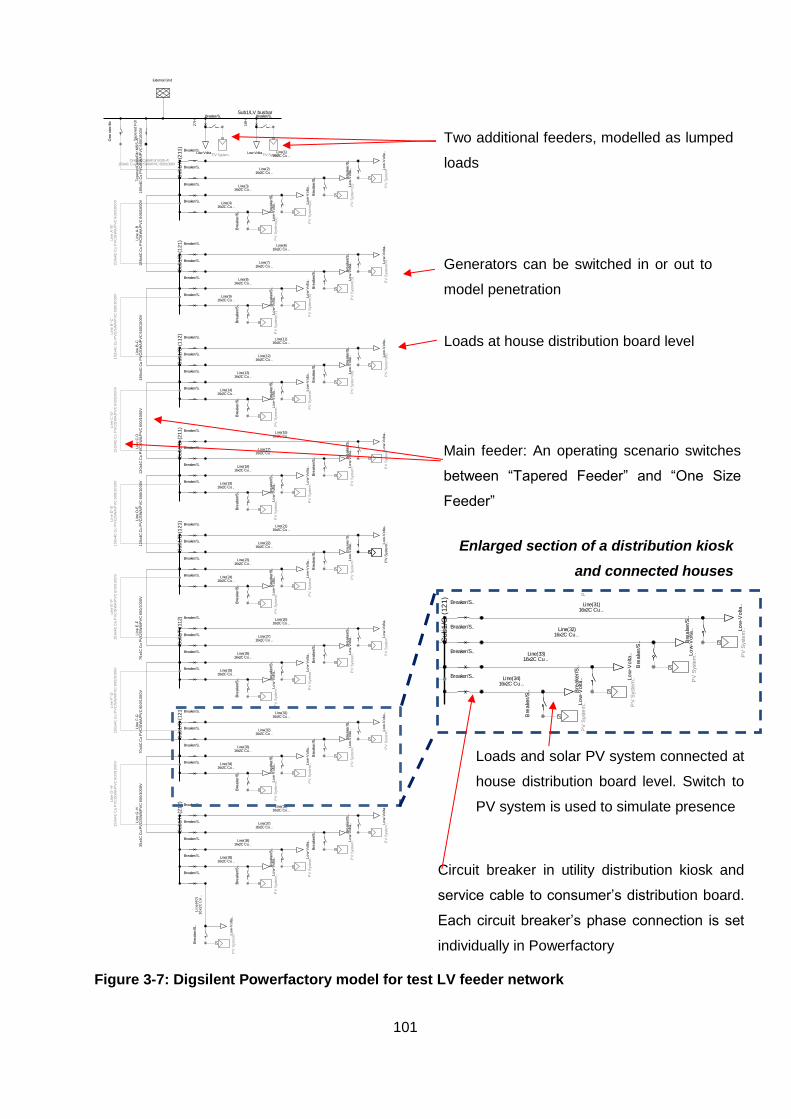
101
Figure 3-7: Digsilent Powerfactory model for test LV feeder network
Inactive
Out of Calculation
De-energised
Su
b1
/H (
21
2)
Sub
1/G
(12
1)
Sub1/F
(112)
Su
b1
/E (
12
1)
Su
b1
/D (
21
1)
Su
b1
/B (
12
1)
Su
b1
/C (
11
2)
Su
b1
/A (
21
1)
Sub1/LV busbar
~
PV System..
~
PV System..
Breaker/S..Breaker/S..Breaker/S..Breaker/S..
Low-Volta..Low-Volta..
18
H
27
H
~
PV
Syste
m..
Bre
ake
r/S
..B
rea
ke
r/S
..
Bre
ake
r/S
..B
rea
ke
r/S
..
~
PV
Syste
m..
Bre
ake
r/S
..B
rea
ke
r/S
..
~
PV
Syste
m..
Bre
ake
r/S
..B
rea
ke
r/S
..
~
PV
Syste
m..
Bre
ake
r/S
..B
rea
ke
r/S
..
~
PV
Syste
m..
Bre
ake
r/S
..B
rea
ke
r/S
..
~
PV
Syste
m..
Bre
ake
r/S
..B
rea
ke
r/S
..
~
PV
Syste
m..
Bre
ake
r/S
..B
rea
ke
r/S
..
~
PV
Syste
m..
Bre
ake
r/S
..B
rea
ke
r/S
..
~
PV
Syste
m..
Bre
ake
r/S
..B
rea
ke
r/S
..
~
PV
Syste
m..
Bre
ake
r/S
..B
rea
ke
r/S
..
~
PV
Syste
m..
Bre
ake
r/S
..B
rea
ke
r/S
..
~
PV
Syste
m..
Bre
ake
r/S
..B
rea
ke
r/S
..
~
PV
Syste
m..
Bre
ake
r/S
..B
rea
ke
r/S
..
~
PV
Syste
m..
Bre
ake
r/S
..B
rea
ke
r/S
..
~
PV
Syste
m..
Bre
ake
r/S
..B
rea
ke
r/S
..
~
PV
Syste
m..
Bre
ake
r/S
..
~
PV
Syste
m..
Bre
ake
r/S
..B
rea
ke
r/S
..
~
PV
Syste
m..
Bre
ake
r/S
..B
rea
ke
r/S
..
~
PV
Syste
m..
Bre
ake
r/S
..B
rea
ke
r/S
..
~
PV
Syste
m..
Bre
ake
r/S
..B
rea
ke
r/S
..
~
PV
Syste
m..
Bre
ake
r/S
..B
rea
ke
r/S
..
~
PV
Syste
m..
Bre
ake
r/S
..B
rea
ke
r/S
..
~
PV
Syste
m..
Bre
ake
r/S
..B
rea
ke
r/S
..
~
PV
Syste
m(9
)
Bre
ake
r/S
..B
rea
ke
r/S
..
~
PV
Syste
m(8
)
Bre
ake
r/S
..B
rea
ke
r/S
..
~
PV
Syste
m(7
)
Bre
ake
r/S
..B
rea
ke
r/S
..
~
PV
Syste
m(6
)B
rea
ke
r/S
..B
rea
ke
r/S
..
~
PV
Syste
m(5
)
Bre
ake
r/S
..B
rea
ke
r/S
..
~
PV
Syste
m(4
)
Bre
ake
r/S
..B
rea
ke
r/S
..
~
PV
Syste
m(3
)
Bre
ake
r/S
..B
rea
ke
r/S
..
~
PV
Syste
m(2
)B
rea
ke
r/S
..B
rea
ke
r/S
..
~
PV
Syste
m(1
)
Lin
e G
'-H
'1
50
x4
C C
u P
VC
/SW
A/P
VC
60
0/1
00
0V
Lin
e F
'-G
'1
50
x4
C C
u P
VC
/SW
A/P
VC
60
0/1
00
0V
Lin
e E
'-F
'1
50
x4
C C
u P
VC
/SW
A/P
VC
60
0/1
00
0V
Lin
e D
'-E
'1
50
x4
C C
u P
VC
/SW
A/P
VC
60
0/1
00
0V
Lin
e C
'-D
'1
50
x4
C C
u P
VC
/SW
A/P
VC
60
0/1
00
0V
Lin
e B
'-C
'1
50
x4
C C
u P
VC
/SW
A/P
VC
60
0/1
00
0V
Lin
e A
'-B
'1
50
x4
C C
u P
VC
/SW
A/P
VC
60
0/1
00
0V
OneSizeCableFdr MSS-A'150x4C Cu PVC/SWA/PVC 600/1000V
On
e s
ize
fd
rO
ne
siz
e fd
r
Bre
ake
r/S
..B
rea
ke
r/S
..
~
PV
Syste
m
Lo
w-V
olta
..
Lin
e(4
0)
16
x2
C C
u ..
Breaker/S..
Lo
w-V
olta
.. Lo
w-V
olta
.. Lo
w-V
olta
.. Lo
w-V
olta
..
Line(39)16x2C Cu ..
Line(38)16x2C Cu ..
Line(37)16x2C Cu ..
Line(36)16x2C Cu ..
Lin
e G
-H3
5x4
C C
u P
VC
/SW
A/P
VC
60
0/1
00
0V
Breaker/S..
Breaker/S..
Breaker/S..
Breaker/S..
Lo
w-V
olta
.. Lo
w-V
olta
.. Lo
w-V
olta
.. Lo
w-V
olta
..
Line(34)16x2C Cu ..
Line(33)16x2C Cu ..
Line(32)16x2C Cu ..
Line(31)16x2C Cu ..
Lin
e F
-G7
0x4
C C
u P
VC
/SW
A/P
VC
60
0/1
00
0V
Breaker/S..
Breaker/S..
Breaker/S..
Breaker/S..
Lo
w-V
olta
.. Lo
w-V
olta
.. Lo
w-V
olta
.. Lo
w-V
olta
..
Line(29)16x2C Cu ..
Line(28)16x2C Cu ..
Line(27)16x2C Cu ..
Line(26)16x2C Cu ..
Lin
e E
-F7
0x4
C C
u P
VC
/SW
A/P
VC
60
0/1
00
0V
Breaker/S..
Breaker/S..
Breaker/S..
Breaker/S..
Lo
w-V
olta
.. Lo
w-V
olta
.. Lo
w-V
olta
.. Lo
w-V
olta
..
Line(24)16x2C Cu ..
Line(23)16x2C Cu ..
Line(22)16x2C Cu ..
Line(21)16x2C Cu ..
Lin
e D
-E1
20
x4
C C
u P
VC
/SW
A/P
VC
60
0/1
00
0V
Breaker/S..
Breaker/S..
Breaker/S..
Breaker/S..
Lo
w-V
olta
.. Lo
w-V
olta
.. Lo
w-V
olta
.. Lo
w-V
olta
..
Line(19)16x2C Cu ..
Line(18)16x2C Cu ..
Line(17)16x2C Cu ..
Line(16)16x2C Cu ..
Lin
e C
-D1
20
x4
C C
u P
VC
/SW
A/P
VC
60
0/1
00
0V
Breaker/S..
Breaker/S..
Breaker/S..
Breaker/S..
Lo
w-V
olta
.. Lo
w-V
olta
.. Lo
w-V
olta
.. Lo
w-V
olta
..
Line(14)16x2C Cu ..
Line(13)16x2C Cu ..
Line(12)16x2C Cu ..
Line(11)16x2C Cu ..
Lin
e B
-C1
85
x4
C C
u P
VC
/SW
A/P
VC
60
0/1
00
0V
Breaker/S..
Breaker/S..
Breaker/S..
Breaker/S..
Lo
w-V
olta
.. Lo
w-V
olta
.. Lo
w-V
olta
.. Lo
w-V
olta
..
Line(9)16x2C Cu ..
Line(8)16x2C Cu ..
Line(7)16x2C Cu ..
Line(6)16x2C Cu ..
Lin
e A
-B1
85
x4
C C
u P
VC
/SW
A/P
VC
60
0/1
00
0V
Breaker/S..
Breaker/S..
Breaker/S..
Breaker/S..
Lo
w-V
olta
.. Lo
w-V
olta
.. Lo
w-V
olta
.. Lo
w-V
olta
..
Line(4)16x2C Cu ..
Line(3)16x2C Cu ..
Line(2)16x2C Cu ..
Line(1)16x2C Cu ..
External Grid
Ta
pe
red
Ca
ble
Fd
r M
SS
-A1
85
x4
C C
u P
VC
/SW
A/P
VC
60
0/1
00
0V
Breaker/S..
Breaker/S..
Breaker/S..
Breaker/S..
Ta
pe
red
Fd
r
DIg
SIL
EN
T
Generators can be switched in or out to
model penetration
Loads at house distribution board level
Main feeder: An operating scenario switches
between “Tapered Feeder” and “One Size
Feeder”
Two additional feeders, modelled as lumped
loads
Inactive
Out of Calculation
De-energised
Su
b1
/H (
21
2)
Sub
1/G
(12
1)
Sub1/F
(112)
Su
b1
/E (
12
1)
Su
b1
/D (
21
1)
Su
b1
/B (
12
1)
Su
b1
/C (
11
2)
Su
b1
/A (
21
1)
Sub1/LV busbar
~
PV System..
~
PV System..
Breaker/S..Breaker/S..Breaker/S..Breaker/S..
Low-Volta..Low-Volta..
18
H
27
H
~
PV
Syste
m..
Bre
ake
r/S
..B
rea
ke
r/S
..
Bre
ake
r/S
..B
rea
ke
r/S
..
~
PV
Syste
m..
Bre
ake
r/S
..B
rea
ke
r/S
..
~
PV
Syste
m..
Bre
ake
r/S
..B
rea
ke
r/S
..
~
PV
Syste
m..
Bre
ake
r/S
..B
rea
ke
r/S
..
~
PV
Syste
m..
Bre
ake
r/S
..B
rea
ke
r/S
..
~
PV
Syste
m..
Bre
ake
r/S
..B
rea
ke
r/S
..
~
PV
Syste
m..
Bre
ake
r/S
..B
rea
ke
r/S
..
~
PV
Syste
m..
Bre
ake
r/S
..B
rea
ke
r/S
..
~
PV
Syste
m..
Bre
ake
r/S
..B
rea
ke
r/S
..
~
PV
Syste
m..
Bre
ake
r/S
..B
rea
ke
r/S
..
~
PV
Syste
m..
Bre
ake
r/S
..B
rea
ke
r/S
..
~
PV
Syste
m..
Bre
ake
r/S
..B
rea
ke
r/S
..
~
PV
Syste
m..
Bre
ake
r/S
..B
rea
ke
r/S
..
~
PV
Syste
m..
Bre
ake
r/S
..B
rea
ke
r/S
..
~
PV
Syste
m..
Bre
ake
r/S
..B
rea
ke
r/S
..
~
PV
Syste
m..
Bre
ake
r/S
..
~
PV
Syste
m..
Bre
ake
r/S
..B
rea
ke
r/S
..
~
PV
Syste
m..
Bre
ake
r/S
..B
rea
ke
r/S
..
~
PV
Syste
m..
Bre
ake
r/S
..B
rea
ke
r/S
..
~
PV
Syste
m..
Bre
ake
r/S
..B
rea
ke
r/S
..
~
PV
Syste
m..
Bre
ake
r/S
..B
rea
ke
r/S
..
~
PV
Syste
m..
Bre
ake
r/S
..B
rea
ke
r/S
..
~
PV
Syste
m..
Bre
ake
r/S
..B
rea
ke
r/S
..
~
PV
Syste
m(9
)
Bre
ake
r/S
..B
rea
ke
r/S
..
~
PV
Syste
m(8
)
Bre
ake
r/S
..B
rea
ke
r/S
..
~
PV
Syste
m(7
)
Bre
ake
r/S
..B
rea
ke
r/S
..
~
PV
Syste
m(6
)B
rea
ke
r/S
..B
rea
ke
r/S
..
~
PV
Syste
m(5
)
Bre
ake
r/S
..B
rea
ke
r/S
..
~
PV
Syste
m(4
)
Bre
ake
r/S
..B
rea
ke
r/S
..
~
PV
Syste
m(3
)
Bre
ake
r/S
..B
rea
ke
r/S
..
~
PV
Syste
m(2
)B
rea
ke
r/S
..B
rea
ke
r/S
..
~
PV
Syste
m(1
)
Lin
e G
'-H
'1
50
x4
C C
u P
VC
/SW
A/P
VC
60
0/1
00
0V
Lin
e F
'-G
'1
50
x4
C C
u P
VC
/SW
A/P
VC
60
0/1
00
0V
Lin
e E
'-F
'1
50
x4
C C
u P
VC
/SW
A/P
VC
60
0/1
00
0V
Lin
e D
'-E
'1
50
x4
C C
u P
VC
/SW
A/P
VC
60
0/1
00
0V
Lin
e C
'-D
'1
50
x4
C C
u P
VC
/SW
A/P
VC
60
0/1
00
0V
Lin
e B
'-C
'1
50
x4
C C
u P
VC
/SW
A/P
VC
60
0/1
00
0V
Lin
e A
'-B
'1
50
x4
C C
u P
VC
/SW
A/P
VC
60
0/1
00
0V
OneSizeCableFdr MSS-A'150x4C Cu PVC/SWA/PVC 600/1000V
On
e s
ize
fd
rO
ne
siz
e fd
r
Bre
ake
r/S
..B
rea
ke
r/S
..
~
PV
Syste
m
Lo
w-V
olta
..
Lin
e(4
0)
16
x2
C C
u ..
Breaker/S..
Lo
w-V
olta
.. Lo
w-V
olta
.. Lo
w-V
olta
.. Lo
w-V
olta
..
Line(39)16x2C Cu ..
Line(38)16x2C Cu ..
Line(37)16x2C Cu ..
Line(36)16x2C Cu ..
Lin
e G
-H3
5x4
C C
u P
VC
/SW
A/P
VC
60
0/1
00
0V
Breaker/S..
Breaker/S..
Breaker/S..
Breaker/S..
Lo
w-V
olta
.. Lo
w-V
olta
.. Lo
w-V
olta
.. Lo
w-V
olta
..
Line(34)16x2C Cu ..
Line(33)16x2C Cu ..
Line(32)16x2C Cu ..
Line(31)16x2C Cu ..
Lin
e F
-G7
0x4
C C
u P
VC
/SW
A/P
VC
60
0/1
00
0V
Breaker/S..
Breaker/S..
Breaker/S..
Breaker/S..
Lo
w-V
olta
.. Lo
w-V
olta
.. Lo
w-V
olta
.. Lo
w-V
olta
..
Line(29)16x2C Cu ..
Line(28)16x2C Cu ..
Line(27)16x2C Cu ..
Line(26)16x2C Cu ..
Lin
e E
-F7
0x4
C C
u P
VC
/SW
A/P
VC
60
0/1
00
0V
Breaker/S..
Breaker/S..
Breaker/S..
Breaker/S..
Lo
w-V
olta
.. Lo
w-V
olta
.. Lo
w-V
olta
.. Lo
w-V
olta
..
Line(24)16x2C Cu ..
Line(23)16x2C Cu ..
Line(22)16x2C Cu ..
Line(21)16x2C Cu ..
Lin
e D
-E1
20
x4
C C
u P
VC
/SW
A/P
VC
60
0/1
00
0V
Breaker/S..
Breaker/S..
Breaker/S..
Breaker/S..
Lo
w-V
olta
.. Lo
w-V
olta
.. Lo
w-V
olta
.. Lo
w-V
olta
..
Line(19)16x2C Cu ..
Line(18)16x2C Cu ..
Line(17)16x2C Cu ..
Line(16)16x2C Cu ..
Lin
e C
-D1
20
x4
C C
u P
VC
/SW
A/P
VC
60
0/1
00
0V
Breaker/S..
Breaker/S..
Breaker/S..
Breaker/S..
Lo
w-V
olta
.. Lo
w-V
olta
.. Lo
w-V
olta
.. Lo
w-V
olta
..
Line(14)16x2C Cu ..
Line(13)16x2C Cu ..
Line(12)16x2C Cu ..
Line(11)16x2C Cu ..
Lin
e B
-C1
85
x4
C C
u P
VC
/SW
A/P
VC
60
0/1
00
0V
Breaker/S..
Breaker/S..
Breaker/S..
Breaker/S..
Lo
w-V
olta
.. Lo
w-V
olta
.. Lo
w-V
olta
.. Lo
w-V
olta
..
Line(9)16x2C Cu ..
Line(8)16x2C Cu ..
Line(7)16x2C Cu ..
Line(6)16x2C Cu ..
Lin
e A
-B1
85
x4
C C
u P
VC
/SW
A/P
VC
60
0/1
00
0V
Breaker/S..
Breaker/S..
Breaker/S..
Breaker/S..
Lo
w-V
olta
.. Lo
w-V
olta
.. Lo
w-V
olta
.. Lo
w-V
olta
..
Line(4)16x2C Cu ..
Line(3)16x2C Cu ..
Line(2)16x2C Cu ..
Line(1)16x2C Cu ..
External Grid
Ta
pe
red
Ca
ble
Fd
r M
SS
-A1
85
x4
C C
u P
VC
/SW
A/P
VC
60
0/1
00
0V
Breaker/S..
Breaker/S..
Breaker/S..
Breaker/S..
Ta
pe
red
Fd
r
DIg
SIL
EN
T
Enlarged section of a distribution kiosk
and connected houses
Loads and solar PV system connected at
house distribution board level. Switch to
PV system is used to simulate presence
Circuit breaker in utility distribution kiosk and
service cable to consumer’s distribution board.
Each circuit breaker’s phase connection is set
individually in Powerfactory

102
3.8.3 Load flow modelling scenarios
LV feeders in residential areas mostly experience peak loading conditions during the evening. As
such, a feeder at high load conditions will not experience an impact from solar PV on the Gauteng
Highveld, but may very well experience some impact in the Western Cape where the sun sets
later.
The baseline for comparison at high load conditions and low load conditions will be with no form
of distributed or embedded generation present.
Suppose the test feeder is somewhere in the Gauteng province where solar PV will have no effect
during high load conditions. A micro wind turbine may still have an effect during the evening peak
and the effects of generating during high load conditions were investigated.
During a typical load condition, solar PV might be at its maximum output, and voltage rise is
expected.
The Herman-Beta method may not necessarily apply during low load conditions, since the load
distribution may be different. An empirical approach may be necessary where an average demand
per household is determined equal to the load profile’s low load around the solar peak.
Simulating renewable power generation at the time of the feeder’s peak, however, will indicate for
instance, what will happen if wind generation is deployed and sufficient wind is available to
produce say 1.5 kW, or 3 kW, or even 9 kW at domestic level.
It was also assumed that utilities may not have control over what consumers do, and the
restrictions as imposed by NRS097 [30] may not be adhered to. The assumption was made that
consumers are ignorant and do not pay attention to NRS 097 and install any size system they
prefer or can afford. Therefore, DG systems larger than 4.6 kW were not modelled as three-phase,
but rather as a 9kW single phase system
The scenarios to be investigated are each of the two feeder configurations (Scenario A1 and
Scenario A2), for both DG active during high demand and low demand scenarios. Generally, solar
PV will be active during low demand periods, but a wind turbine may be generating electricity
during the evening peak.

103
Chapter summary
In this chapter, a simulation tool was described that allows the ability to simulate changes in
ADMD’s after intervention of EEDSM and RPP type projects.
A load flow model was also described through which the impact on network performance can be
quantified. The next chapter presents the findings and results.

104
Chapter 4 Findings and results
Introduction
In the previous chapter, the design of analysis and simulation tools were described in an effort to
quantify the impact EEDSM and DG have on our grid networks.
Load profile validation and verification
4.2.1 General considerations
Validation in plain terms is defined as doing “the right thing”, while verification is defined in plain
terms as doing “the thing right”.
When applying it to the process at hand, it means that validation focuses on the correlation of the
calculated profile with actual profiles (to demonstrate that it is the right thing), and verification
focuses on whether the calculations derived are done right (i.e. how it measures up to known
theory and expected results). Aspects of validation and verification are summarized in the
following table.
Table 4-1: Validation and verification methodology
Test aspect Validation
Doing the right thing
Verification
Doing it right
Load profile
shape
Is the reference load profile
used for comparing purposes
appropriate?
Does the simulated profile compare or
correlate with the reference profile?
ADMD Is it calculated using correct
formula?
Does ADMD reduce as the number of
consumers increase?
Diversity /
Coincidence
Is it calculated using correct
formula?
Does coincidence decrease or diversity
increase as the number of consumers
increase?
Load factor Is it calculated using correct
formula?
Is the load factor representative of
expected loads, i.e. not too high, or not
too low?

105
Test aspect Validation
Doing the right thing
Verification
Doing it right
Applying green
measures
Are the typical measures to be
investigated representative of
what one would expect to find
on a domestic network?
Does the peak load reduce when geysers
for instance are omitted (e.g. replaced
with solar geysers without electrical back-
up elements)?
4.2.2 Load profile shape
A reference load profile was selected from available one-minute load profiles representing mostly
domestic load. In any load measured at substation level for predominantly domestic load, there
will always be non-domestic load such as street and area lighting, possibly traffic signals, a few
small shops, schools and other community facilities such as churches, a police station etc.
The network as measured in the reference curve, has ripple control present and the effects thereof
is easily demonstrated comparing days when ripple control is active (e.g. weekdays) against days
when the ripple control is inactive (e.g. typical Sunday). An inactive day was selected as reference
curve, although any of the other days can also be selected by scrolling on the interface through
the 31 imported daily profiles. May 2013 recorded the coldest day during 2013, or at least the
maximum demand for many utilities. From experience, the coldest week of the year on the South
African Highveld is experienced in July, and normally coincides with the annual Eskom maximum
demand.
The calculated composite load profile, consisting of a domestic load component and a non-
domestic load component, is compared to two reference profiles as follows:

106
Notes pertaining to figures
on this page:
Number of households
simulated = 500.
Reference curve for top
graph (a) = weekday curve
with ripple control active.
Reference curve for
bottom graph (b) = Sunday
curve with no load control.
Simulated curve =
weekday curve.
In the top graph the
morning profile rise and
the evening load coincides
with the reference curve.
For the bottom reference
profile, the late rising of
people on a Sunday as
opposed to a normal
weekday is observed.
However, what is
important here is the
coincidence of the rise and
drop of the evening peak.
The high noon peak for the
reference curve is due to
home cooking on a
Sunday, but for the
weekday curve, it is not
applicable.
Figure 4-1: Calculated load profile (black) compared to a reference curve (magenta) with
load control (sub-figure a) and without load control (sub-figure b)
(a)
(b)

107
The selected reference profiles were scaled on the y-axis such that its maximum demand equals
the simulated profile maximum demand (without interventions).
It is possible that the non-domestic load in the reference load profile is higher than anticipated. It
was not verified. The “double hump” load profile constructed (black line) is considered satisfactory
for further use. Only the domestic portion (blue line) is of interest in this study and the non-
domestic load portion is not considered further. The reference curve is only used to verify that the
calculated composite load profile (black line) is representative (i.e. as to where it calculates the
peaks compared to an actual situation).
4.2.3 ADMD
It is expected that ADMD will decay as the number of households increase up to a point where
after it does not decay substantially. From the simulated results, the following scatter plot is
derived:
Figure 4-2: ADMD vs number of households (simulated)
0
1
2
3
4
5
6
7
8
0 100 200 300 400 500
AD
MD
(kVA
)
Number of households
ADMD per number of households
ADMD

108
The graph shows ADMD calculated results from 744 case study profiles ranging from 10 to 500
households. It is evident from the graph that the ADMD decays as the number of households
increase and stabilizes for high household numbers. The number of low ADMDs for households
below 50 is simply an indication that ADMD is in general not very accurate when based on small
quantities due to lack of diversity. Even NRS034 [3] indicates an upward adjustment of ADMD
(refer to Equation 33), to compensate for a lack of diversity.
It is concluded that the study cases and model provide useful ADMD values for comparison
purposes.
The same case study data is used for all graphs following.
4.2.4 Diversity / Coincidence
It is expected that coincidence will decay as the number of households increase up to a point,
where after it does not decay substantially. Figure 4-3 illustrates a coincidence scatter plot from
the simulated results:
Figure 4-3: Coincidence vs number of households (simulated)
0.40
0.45
0.50
0.55
0.60
0.65
0.70
0.75
0.80
0 100 200 300 400 500
Coin
cid
en
ce
Number of households
Coincidence per number of households
Coincidence

109
From the simulated results, it is evident that the coincidence indeed decays over time and reaches
a stabilizing level. The simulation achieves slightly higher than anticipated results. It was expected
to stabilize around 0.42, based on experience.
4.2.5 Load factor
Load factor (average demand divided by maximum demand) is a function of the maximum
demand and it is expected that the load factor will follow the stabilizing pattern of the ADMD,
which is also based on the maximum demand. The calculated results from the simulated profiles
in the study case files are observed on the following scatter plot:
Figure 4-4: Load factor vs number of households (simulated)
The load factor is within acceptable limits for affluent residents.
0.3
0.4
0.5
0.6
0 100 200 300 400 500
Load
facto
r
Number of households
Load factor per number of households
Load factor

110
4.2.6 Effect of “green” measures
Figure 4-1 in Paragraph 4.2.2 indicated a load curve in a red line after adjustment. In this instance,
the following was applicable:
• 3 kW solar PV for 20% of the 500 households
• 100% electrical stoves replaced by gas stoves
• 100% replacement of all electrical geysers per household with solar geysers.
From the adjusted profile, it is evident that the profile reduces as electricity is generated by a solar
PV system, especially during the middle of the day, and that the peaks are considerably lower,
as will be expected when electrical geysers are replaced with solar geysers. The reduction
technique applied therefore is acceptable for the purposes of modelling. Since the base profile
was acceptable, it can be concluded that the calculation of an adjusted profile provides
satisfactory results for comparison to conventional scenarios.
4.2.7 Validation and verification conclusion
It can be concluded that the simulation produces satisfactory results for studying the effects of
renewable energy, energy efficiency and demand side management measures on planning
parameters such as ADMD, coincidence and load factor.
Analysis of results obtained through appliance model simulation
4.3.1 Case studies
The following scenarios were investigated with the appliance model simulation tool.
Table 4-2: Study scenarios with appliance model simulation tool
Study scenario PV penetration level
PV Size Electric stoves replaced with
gas stoves
Electric geysers
replaced with solar geysers
A 10% 1.5 kW X
B 10% 1.5 kW X
C 10% 1.5 kW X X

111
Study scenario PV penetration level
PV Size Electric stoves replaced with
gas stoves
Electric geysers
replaced with solar geysers
D 20% 1 kW X X
E 20% 3 kW X X
F 40% 3 kW X X
G 50% 5 kW X X
These scenarios were chosen as follows:
• A, B & C: study the effects of replacement of appliances with appliances reducing energy
and demand such as replacement of electric stoves and geysers with gas appliances. The
PV effect was kept the same.
• D & E: Keep PV penetration level the same, but vary the PV size.
• E & F: Keep PV size the same, but vary penetration level.
• G: Simulate high PV penetration with high PV size.
In Germany, the maximum solar PV penetration level reached on a macro scale is 45% [34], but
on a localized scale, generation may exceed demand.
On the graphs that follow in Figures 4-5 to 4-13, the colours assigned to these scenarios are:
• Baseline = Grey circles
• A = Green
• B = Purple
• C = Cyan
• D = Red
• E = Orange
• F = Dark blue
• G = Maroon.
4.3.2 Impact of green measures on ADMD
The ADMD for the profile without intervention was illustrated in Figure 4-2. The same data in the
graph below is represented by the grey circles. For each profile calculated, a “green” profile was
also calculated.

112
Figure 4-5: Effect of various green measures on ADMD, compared to a baseline without
any interventions
The impact of various measures on ADMD is illustrated in figures 4-6 and 4-7.
2
3
4
5
6
7
8
0 100 200 300 400 500
AD
MD
(kVA
/ h
ou
seh
old
)
Number of households
ADMD per number of households
No intervention A B C D E F G
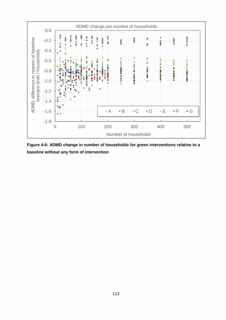
113
Figure 4-6: ADMD change in number of households for green interventions relative to a
baseline without any form of intervention
-1.8
-1.6
-1.4
-1.2
-1.0
-0.8
-0.6
-0.4
-0.2
0.0
0 100 200 300 400 500
AD
MD
diffe
ren
ce in
resp
ect of
baselin
e
scen
ario (
kVA
/ h
ou
seh
old
)
Number of households
ADMD change per number of households
A B C D E F G

114
Figure 4-7: Percentage change in ADMD per number of households in the simulation
group relative to a baseline without any form of intervention
4.3.3 Impact of green initiatives on coincidence
The impact on coincidence is expressed in Figures 4-8 and 4-9.
-40%
-35%
-30%
-25%
-20%
-15%
-10%
-5%
0%
0 100 200 300 400 500
Ch
an
ge in
resp
ect of
baselin
e s
cen
ario
(% k
VA
/ h
ou
seh
old
)
Number of households
% ADMD change per number of households
A B C D E F G

115
Figure 4-8: Impact on coincidence for green interventions relative to a baseline without
any form of intervention
-0.10
-0.05
0.00
0.05
0.10
0.15
0 100 200 300 400 500
Coin
cid
en
ce d
iffe
ren
ce in
resp
ect
of a b
aselin
e s
cen
ario
Number of households
Change in coincidence per number of households
A B C D E F G

116
Figure 4-9: Percentage coincidence change for green interventions relative to a baseline
without any form of intervention
4.3.4 Impact of green initiatives on load factor
The impact on load factor is observed in Figures 4-10 and 4-11.
-25%
-20%
-15%
-10%
-5%
0%
5%
10%
15%
0 100 200 300 400 500
Coin
cid
en
ce c
han
ge in
resp
ect
of
a b
aselin
e s
cen
ario (
%)
Number of households
% Change in coincidence per number of households
A B C D E F G

117
Figure 4-10: Impact on load factor for green interventions relative to a baseline without
any form of intervention
-0.35
-0.30
-0.25
-0.20
-0.15
-0.10
-0.05
0.00
0.05
0 100 200 300 400 500
Load
facto
r d
iffe
ren
ce in
resp
ect
of
a b
aselin
e s
cen
ario
Number of households
Change in load factor per number of households
A B C D E F G

118
Figure 4-11: Percentage change in load factor for green interventions relative to a
baseline without any form of intervention
4.3.5 Summary of initiatives and interdependent impact
The impact of the various green initiatives on ADMD, coincidence and load factor is summarized
in Table 4-3.
Table 4-3: Impact on parameters for simulations of 100 households or more
Study scenario
PV penetration
level
PV Size
kW
Gas stoves
Solar geysers
ADMD change
kVA
ADMD change
%
Coin-cidence change
%
Load factor
change %
A-Green 10% 1.5 X -0.52 to
-0.85
-11 to
-20
-1 to
-11
-4 to
-13
B-Purple 10% 1.5 X -0.1 to
-0.36
-2 to
-8
0 to
+5
-3.5 to
+2.4
C-Cyan 10% 1.5 X X -0.66 to
-1.09
-16 to
-28
-1 to
0
-1 to
-10
-180%
-160%
-140%
-120%
-100%
-80%
-60%
-40%
-20%
0%
20%
0 100 200 300 400 500
Load
facto
r ch
an
ge in
resp
ect
of
a b
aselin
e s
cen
ario (
%)
Number of households
% Change in load factor per number of households
A B C D E F G

119
Study scenario
PV penetration
level
PV Size
kW
Gas stoves
Solar geysers
ADMD change
kVA
ADMD change
%
Coin-cidence change
%
Load factor
change %
D-Red 20% 1 X X -0.74 to
-1.18
-18 to
-29
-10 to
+2.5
-2 to
-12
E-Orange
20% 3 X X -0.73 to
-1.09
-18 to -29
-9 to
0
-24 to
-9
F-Dark blue
40% 3 X X -0.69 to
-1.07
-16 to
-27
-9 to
0
-25 to
-53
G-Maroon
50% 5 X X -0.63 to
-1.00
-14 to
-26
-13 to
-1
-54 to
-127
Negative change indicates a reduction in value. This table is perhaps better illustrated graphically
in Figure 4-12 (a)-(d):

120
Figure 4-12: Impact of various green interventions: (a) ADMD change in kVA, (b) ADMD % change, (c) Coincidence % change and (d)
Load factor percentage change
-1.4 -1.2 -1 -0.8 -0.6 -0.4 -0.2 0
A
B
C
D
E
F
G
ADMD variation range relative to baseline (kVA)
Sce
na
rio
(a)
-35 -30 -25 -20 -15 -10 -5 0
A
B
C
D
E
F
G
ADMD variation range relative to baseline (%)
Sce
na
rio
(b)
-15 -12 -9 -6 -3 0 3 6
A
B
C
D
E
F
G
Coincidence variation range relative to baseline (%)
Sce
na
rio
(c)
-140 -120 -100 -80 -60 -40 -20 0
A
B
C
D
E
F
G
Load factor variation range relative to baseline (%)S
ce
na
rio
(d)
PV Size
kW
A 10% 1.5 X
B 10% 1.5 X
C 10% 1.5 X X
D 20% 1 X X
E 20% 3 X X
F40% 3 X X
G 50% 5 X X
Scenario PV
penetra-
tion
level
Gas
stoves
Solar
geysers

121
The load factor was further investigated in respect of coincidence. The graphs in Figure 4-12 illustrate the findings:
Key for scenarios of intervention combinations:
Figure 4-13: Additional findings: (a) ADMD vs Load factor; (b) ADMD vs Coincidence; (c) Coincidence vs Load factor
2
3
4
5
6
7
8
9
0.1 0.2 0.3 0.4 0.5 0.6
AD
MD
(kVA
/ h
ou
seh
old
)
Load factor
ADMD vs Load factor
No intervention A B C D E F G (a)
2
3
4
5
6
7
8
9
0.4 0.5 0.6 0.7 0.8
AD
MD
(kVA
/ h
ou
seh
old
)
Coincidence
ADMD vs Coincidence
No intervention A B C D E F G (b)
0.4
0.5
0.6
0.7
0.8
0.1 0.2 0.3 0.4 0.5 0.6
Coin
cid
en
ce
Load factor
Coincidence vs Load factor
No intervention A B C D E F G (c)
PV Size
kW
A 10% 1.5 X
B 10% 1.5 X
C 10% 1.5 X X
D 20% 1 X X
E 20% 3 X X
F40% 3 X X
G 50% 5 X X
Scenario PV
penetra-
tion
level
Gas
stoves
Solar
geysers

122
In summary, the following conclusions can be drawn:
Table 4-4: Summary of impact to ADMD, coincidence and load factor due to
implementation of various green initiatives
Variance in or application of green initiatives
Impact on ADMD, Coincidence and Load factor
Replacing electrical geysers
with solar geysers
Largest reduction in ADMD through appliance replacement.
Increase in coincidence, i.e. provide less diversity. Less
coincidence is usually associated with higher ADMDs.
Slight decrease in load factor due to lower energy usage.
Replacing electrical stoves with
gas stoves
Reduces ADMD only slightly.
Almost the same deviation from original coincidence in either
direction. It is concluded that replacement of stoves with gas
stoves does not significantly impact coincidence.
Slight decrease in load factor due to lower energy usage.
Replacing electrical geysers
with solar geysers and
electrical stoves with gas
stoves
Combined effect yields significant ADMD reduction.
Combined effect causes little to no change in coincidence.
Small change in load factor.
Increase solar PV penetration
level
ADMD and coincidence levels do not change if reverse power
flow does not cause ADMD to shift from evening peak to
midday peak.
Load factor reduces significantly due to reduction in energy
consumption
Increase solar PV size ADMD and coincidence levels do not change if reverse power
flow does not cause ADMD to shift from evening peak to
midday peak.
Load factor reduces significantly due to reduction in energy
consumption.

123
Variance in or application of green initiatives
Impact on ADMD, Coincidence and Load factor
Increase solar PV penetration
level and size
ADMD and coincidence levels do not change if reverse power
flow does not cause ADMD to shift from evening peak to
midday peak.
Load factor reduces significantly due to reduction in energy
consumption
4.3.6 Analysis of the distribution of peak current
The model also allows for the analysis of the distribution of currents. The theory associated with
the Herman-Beta voltage drop method states that the currents at peak time follows a Beta
distribution curve. Using the T and Adjusted_T matrices, the current distribution at the time of
coincident maximum demand can be observed. The current distribution is best viewed in the form
of a histogram, where the frequency of occurrence of a current can be displayed against the
current. The model assumes that the load has no dependency on voltage.
In the diagrams in Table 4-5, the peak current distribution is displayed in blue for a conventional
case (no “green” measures), while the current distribution when adjustments through “green”
measures are made, is displayed in red. Where the two scenarios overlap, it displays in maroon.
Table 4-5: Distribution of peak currents under various scenarios
Distribution of peak currents Scenario summary
Conventional ADMD: 4.7 kVA Adjusted ADMD: 3.97 kVA Conditions for adjusted curve: Solar PV 3 kW, 20% penetration Two geysers replaced with solar geysers. Stove replaced with gas stove. Conventional load factor: 0.47 Adjusted load factor: 0.39 Conventional coincidence: 0.51 Adjusted coincidence: 0.56

124
Distribution of peak currents Scenario summary
Conventional ADMD: 4.8 kVA Adjusted ADMD: 3.96 kVA Conditions for adjusted curve: Solar PV 5 kW, 50% penetration. Two geysers replaced with solar geysers. Stove replaced with gas stove. Conventional load factor: 0.46 Adjusted load factor: 0.24 Conventional coincidence: 0.53 Adjusted coincidence:0.57
Conventional ADMD: 4.8 kVA Adjusted ADMD: -7.3 kVA Solar PV 7.5 kW 100% penetration Two geysers replaced with solar geysers. Stove replaced with gas stove. Conventional load factor: 0.46 Adjusted load factor: 0.13 Conventional coincidence: 0.54 Adjusted coincidence:1.0

125
Distribution of peak currents Scenario summary
Conventional ADMD: 5.9 kVA Adjusted ADMD: -7.45 kVA Solar PV 7.5 kW 100% penetration Two geysers replaced with solar geysers. Stove replaced with gas stove. Conventional load factor: 0.41 Adjusted load factor: 0.1 Conventional coincidence: 0.59 Adjusted coincidence: 0.94 Note: The narrow distribution cause the red bars to display the black boundaries close to one another and appears black.
From these results, the following observations are made:
• For the first and second graphs, there is a slight shift towards the left on the graph from the
conventional scenario to the adjusted load profile scenario. The mean of a beta distribution
represents the ADMD, and a mean shifting left is indicative of an ADMD reduction, which was
confirmed through calculation.
• It is also observed that for the first and second graphs in the table, the load factor decreases,
and the coincidence increases. An increase in coincidence is indicative of the reduction in
diversity. With less geysers and stoves in the network, there is less variability in the load
composition as seen from a supply transformer point of view.
• For the third and fourth graphs in the table above, there is a total lack of diversity when the
peak currents flow in the reverse direction. The lack of diversity is observed through the lack
of a wide distribution of currents. A larger number of the households draw the same current.
The peak has shifted from 18:00 to 12:00 due to solar PV power in excess of own usage, and
excess power is exported to the grid. Since this is the case in 100% of the households in the
simulation, all the excess energy will flow back to MV/LV transformer and into the MV network.
This may lead to LV feeder overloading in the reverse direction.

126
Load flow analysis
4.4.1 Analysis presented previously
The test feeder system in Chapter 3 was analysed in ReticMaster and presented in a paper at the
AMEU convention in 2014, a paper delivered as part of this research [1]. The paper investigated
the effects of increased ADMD as a result of ripple control and basic solar PV effects. In
Reticmaster, the generated PV power was modelled as a pure active power generator without
any reactive power capabilities. This is typical of an inverter with cos-phi control set at unity power
factor where the current generated is in phase with the voltage.
However, Reticmaster does not have built-in inverter control functions, and Digsilent Powerfactory
was used to investigate different forms of inverter control algorithms. This allowed for the
investigation of inverters delivering reactive power, even for RPP categories A1 and A2
Digsilent Powerfactory allows for different forms of control, such as Q-control, Q-V control, Q-I
control etc. The effects on voltage due to the deployment of different types of inverters or control
algorithms were studied. The load flow studies also allow for the investigation of the research
questions.
Table 4-6 below lists the scenarios investigated for two test feeders, a tapered cable feeder and
a one size cable feeder, under high and low load conditions.
Table 4-6: Load flow scenarios
Scenario No.
Scenario High load
Tapered feeder
High load
One size feeder
Low load
Tapered feeder
Low load
One size feeder
A1 & 2 No renewables (baseline)
HL-A1 HL-A2 LL-A1 LL-A2
E1 One DG unit close to transformer – 3 kW
HL-E1 LL-E1
E3 One DG unit midway along feeder – 3 kW
HL-E3 LL-E3
E2 One DG unit at the end of the feeder – 3 kW
HL-E2 LL-E2

127
Scenario No.
Scenario High load
Tapered feeder
High load
One size feeder
Low load
Tapered feeder
Low load
One size feeder
C, D 100% DG penetration –
3 kW
HL-D2,3,4,6,7 HL-C2,3,4,6,7 LL-D2,3,4,6,7 LL-C2,3,4,6,7
F, G 100% DG penetration –
9 kW
HL9-G2,3,4,6,7 HL9-F2,3,4,6,7 LL9-G2,3,4,6,7 LL9-F2,3,4,6,7
Control Algorithms 2, 3, 4, 6 and 7 for scenarios C, D, F and G in Table 4-6 are:
• 2: Voltage Q-droop: Reactive power is controlled proportionally to the voltage deviation
from a set-point.
• 3: Voltage Iq-droop: Reactive current is controlled proportionally to the voltage deviation
from a set-point.
• 4: Constant Q: The active and reactive power outputs are fixed according to user criteria
specified.
• 6: Q(V) characteristic: Reactive power controller with a variable set-point. Within the set-
point voltage limits, the reactive power output is maintained.
• 7: Cos phi (P) characteristic: Power factor controller.
Methods 1 and 5 in Digsilent Powerfactory were not investigated. Method 1 is for constant voltage
control, where the voltage is controlled by varying the reactive power to maintain a setpoint
voltage at the busbar. Method 5 is a Q(P) characteristic where the reactive power is varied
according to the power output of the inverter.
Residential PV systems are generally controlled at unity power factor and the inverter will provide
active power only to the network. Larger generation plant is required to be able to implement
multiple control algorithms and the system operator may switch between these control functions.
4.4.2 Baseline analysis
To compare results, load flow studies under high and low load conditions were conducted for the
two test feeders (tapered cable size feeder, and one cable size feeder) as per the scenarios listed

128
in Table 4-6. Figures 4-14 and 4-15 illustrate the baseline voltage profiles along the two test
feeders (tapered feeder and one-size feeder) under high and low load conditions respectively.
The analysis was done in Digsilent Powerfactory, using the unbalanced low voltage load flow
settings. The coincidence factors required for high load conditions and low load conditions were
calculated as follows:
• For high load conditions: ADMD = 13.8 kVA maximum demand x coincidence factor of
0.384058 = 5.3 kVA per house. 13.8 kVA is equivalent to a 60 A single-phase connection
at 230 V at unity power factor. This represents the evening load.
• For low load conditions: Demand = 13.8 kVA maximum demand x coincidence factor of
0.17 = 2.346 kVA per house. This represents the midday load as baseline before adding
solar PV to the network.
Of the two test feeder systems under high load conditions, the tapered cable feeder performed
the worst although, both comply with legal limits (i.e. a voltage above 0.9 p.u. at the house).
A notable slight voltage rise in the blue phase is observed at the end of the feeder without any
form of DG present. This was somewhat unexpected as one expects the voltage to drop
continuously over the feeder length and this was noted in both Reticmaster and Digsilent
Powerfactory. It can only be concluded that it is caused by a momentary unbalance at that
particular point along the feeder.

129
0.60000.48000.36000.24000.12000.0000 [km]
1.13
1.08
1.03
0.98
0.93
0.88
[p.u.]
m:u:A m:u:B
Line-Ground Voltage, Magnitude C
Y1 = 0.900 p.u.
Y1 = 1.000 p.u.
Y1 = 1.100 p.u.
DIg
SIL
EN
T
0.60000.48000.36000.24000.12000.0000 [km]
1.13
1.08
1.03
0.98
0.93
0.88
[p.u.]
m:u:A m:u:B
Line-Ground Voltage, Magnitude C
Y1 = 0.900 p.u.
Y1 = 1.000 p.u.
Y1 = 1.100 p.u.
DIg
SIL
EN
T
Figure 4-14: Baseline Digsilent Powerfactory voltage profile for the red, white and blue
phases respectively along test feeder under high load conditions for a) tapered feeder,
and b) one-size feeder
(a)
(b)
Voltage (
p.u
.)
Voltage (
p.u
.)
Feeder length (km)

130
0.60000.48000.36000.24000.12000.0000 [km]
1.13
1.08
1.03
0.98
0.93
0.88
[p.u.]
m:u:A m:u:B
Line-Ground Voltage, Magnitude C
Y1 = 0.900 p.u.
Y1 = 1.000 p.u.
Y1 = 1.100 p.u.
DIg
SIL
EN
T
0.60000.48000.36000.24000.12000.0000 [km]
1.13
1.08
1.03
0.98
0.93
0.88
[p.u.]
m:u:A m:u:B
Line-Ground Voltage, Magnitude C
Y1 = 0.900 p.u.
Y1 = 1.000 p.u.
Y1 = 1.100 p.u.
DIg
SIL
EN
T
Figure 4-15: Baseline Digsilent Powerfactory voltage profile for the red, white and blue
phases respectively along test feeder under low load conditions for a) tapered feeder,
and b) one-size feeder
(a)
(b)
Voltage (
p.u
.)
Voltage (
p.u
.)
Feeder length (km)

131
4.4.3 Comparison of results with different DG control algorithms: voltage
Even though solar PV will generate very little to nothing during the evening peak (high demand),
other forms of DG may be present, such as micro wind turbines. The impact to voltage at the end
of LV feeders for the two test feeder systems, when adding DG, were investigated considering
various DG inverter control algorithms and penetration levels (refer to Table 4-6 for scenario
descriptions). The results compared against the baselines are illustrated in Figure 4-16.
Figure 4-16: Comparison of various inverter control methods and sizes for a) high load
conditions and b) low load conditions. Red arrows point to violation of voltage limits.
0.80
0.85
0.90
0.95
1.00
1.05
1.10
1.15
HL-
A1
HL-
A2
HL-
C2
HL-
C3
HL-
C4
HL-
C6
HL-
C7
HL-
D2
HL-
D3
HL-
D4
HL-
D6
HL-
D7
HL-
E1
HL-
E2
HL-
E3
HL9
-F2
HL9
-F3
HL9
-F4
HL9
-F6
HL9
-F7
HL9
-G2
HL9
-G3
HL9
-G4
HL9
-G6
HL9
-G7
Vo
ltag
e (p
er u
nit
)
Scenarios
Comparison of voltage at end of a LV feeder under high load conditions with DG (various control options) at 100% penetration (3 & 9 kW units) against a baseline
without DG
Phase A Phase B Phase C At house Vmin Vmax
0.80
0.85
0.90
0.95
1.00
1.05
1.10
1.15
LL-A
1
LL-A
2
LL-C
2
LL-C
3
LL-C
4
LL-C
6
LL-C
7
LL-D
2
LL-D
3
LL-D
4
LL-D
6
LL-D
7
LL-E
1
LL-E
2
LL-E
3
LL9
-F2
LL9
-F3
LL9
-F4
LL9
-F6
LL9
-F7
LL9
-G2
LL9
-G3
LL9
-G4
LL9
-G6
LL9
-G7
Vo
ltag
e (p
er u
nit
)
Scenario
Comparison of voltage at end of a LV feeder under low load conditions with DG (various control options) at 100% penetration (3 & 9 kW units) against a baseline
without DG
Phase A Phase B Phase C At house Vmin Vmax
(a)
(b)

132
Scenarios A1 and A2 are the baseline scenarios for the tapered and one-cable-size feeders
respectively. Under high load conditions, adding one 3 kW LV generator close to the transformer
(scenario HL-E1), results in a voltage at the end of the feeder below 0.9 p.u. at the distribution
kiosk and at the house on one of the phases.
Under low load conditions, the voltage at the end of the feeder rises once DG is introduced. As
the size of DG increases, the voltage may rise to the point where the upper voltage limit is reached
or exceeded (see scenarios LL9-F4 and LL9-G4).
4.4.4 Comparison of results with different DG control algorithms: current
The impact on the current carrying capacity of the cable for the test feeders for the various
scenarios evaluated is graphically illustrated in Figures 4-17 and 4-18 for high load conditions,
and Figures 4-19 and 4-20 for low load conditions.
Figure 4-17: Cable loading (percentage of rated current for the highest loaded phase)
along feeder for the tapered feeder under high load conditions
0
20
40
60
80
100
120
M/S
ub-A
A-B
B-C
C-D
D-E
E-F
F-G
G-H
Cab
le c
urr
en
t lo
ad
ing
(% o
f ra
ted
cu
rren
t)
Cable section
Cable loading along feeder (max. phase per section): tapered feeder
HL-A1 HL-D2 HL-D3 HL-D4 HL-D6 HL-D7 HL-E1
HL-E2 HL-E3 HL9-G2 HL9-G3 HL9-G4 HL9-G6 HL9-G7

133
Figure 4-18: Cable loading (percentage of rated capacity for the highest loaded phase) for
the one-size feeder under high load conditions
0
20
40
60
80
100
120
M/S
ub-A
A-B
B-C
C-D
D-E
E-F
F-G
G-H
Cab
le c
urr
en
t lo
ad
ing
(% o
f ra
ted
cu
rren
t)
Cable section
Cable loading along feeder (max. phase per section): one size feeder
HL-A2 HL-C2 HL-C3 HL-C4 HL-C6 HL-C7
HL9-F2 HL9-F3 HL9-F4 HL9-F6 HL9-F7
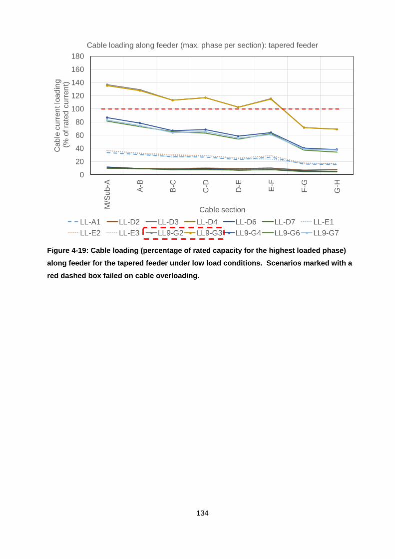
134
Figure 4-19: Cable loading (percentage of rated capacity for the highest loaded phase)
along feeder for the tapered feeder under low load conditions. Scenarios marked with a
red dashed box failed on cable overloading.
0
20
40
60
80
100
120
140
160
180
M/S
ub-A
A-B
B-C
C-D
D-E
E-F
F-G
G-H
Cab
le c
urr
en
t lo
ad
ing
(% o
f ra
ted
cu
rren
t)
Cable section
Cable loading along feeder (max. phase per section): tapered feeder
LL-A1 LL-D2 LL-D3 LL-D4 LL-D6 LL-D7 LL-E1
LL-E2 LL-E3 LL9-G2 LL9-G3 LL9-G4 LL9-G6 LL9-G7

135
Figure 4-20: Cable loading (percentage of rated capacity for the highest loaded phase) for
the one-size feeder under low load conditions. Scenarios marked with a red dashed box
failed on cable overloading.
Under high load conditions, injecting large quantities of energy from the load’s side does not
adversely affect the cables in terms of their rating. Should DG larger than 9 kW be deployed,
problems closer to the transformer may be experienced.
Under low load conditions the cable will be overloaded due to power flow in the reverse direction
when deploying large DG systems, for example a 9 kW solar PV system at 100% penetration
level, should inverters be capable of Voltage Q-droop and Voltage Iq-droop control algorithms be
utilized. 100% penetration of 3 kW systems will typically not cause problems in a 5.3 kVA ADMD
conventional network.
Similar than the tapered feeder, Voltage Q-droop and Voltage Iq-droop control algorithms for large
DG systems deployed in residential systems, for example 100% penetration of 9 kW solar PV
systems, also cause high cable loading due to reverse power flow.
Assuming that the utility was not consulted in the implementation of a large PV system
implementation in a community, it is necessary to carefully consider past protection philosophies.
0
20
40
60
80
100
120
140
160
180
M/S
ub-A
A-B
B-C
C-D
D-E
E-F
F-G
G-H
Cab
le c
urr
en
t lo
ad
ing
(% o
f ra
ted
cu
rren
t)
Cable section
Cable loading along feeder (max. phase per section): one size feeder
LL-A2 LL-C2 LL-C3 LL-C4 LL-C6 LL-C7
LL9-F2 LL9-F3 LL9-F4 LL9-F6 LL9-F7

136
Considering the currents that can flow under overloaded cable conditions by studying Figure 4-
21 below.
Figure 4-21: Protection device arrangement for a tapered and one-size LV cable feeder
The protection arrangement for both feeders are acceptable in the industry. A municipality in the
North-West province of South Africa implements the one-size cable feeder philosophy with
aluminium primary LV cables. The circuit breaker at the transformer protects the full cable. In a
tapered cable feeder system, a circuit breaker is required each time the cable size is reduced.
For a 9 kW system, where the consumers have implemented single phase systems in contrast to
the Grid Code requirement of a three-phase system, the original 60 A or 80 A circuit breakers are
still adequately rated for current flowing into the grid.
The current direction for the primary cables is reversed, and the circuit breaker initially specified
to protect the cable downstream from it is now located downstream from the cable it must protect.
A circuit breaker in general will trip at 130% of its current rating (In). The cable will be subject to a
higher current for a while. For the cable overload scenario in figure 4-20, the following question
arises: if CBTRF is a 250 A circuit breaker, does the cable burn off before the circuit breaker trips?
If all feeders on the transformer exceed their limits by the same margin, the design current

137
capacity of the transformer is exceeded. NRS097 attempts to prevent exactly this scenario by
limiting LV current flowing to the MV network.
To determine the burn-off time of the cable, the following formula is generally used:
𝐼𝑆𝐶 = 𝐾 × 𝐴
√𝑡 ... ( 37 )
Where
ISC = Short circuit current in ampere
t = duration of short circuit in seconds
K = a constant depending on the conductor material used. K =
115 for copper PVC / SWA / PVC cables and 76 for
aluminium PVC /SWA /PVC cables.
A = cable cross section in mm2.
Replacing the short circuit current ISC with the current that will flow under overload conditions (I),
and rewriting Equation 37, the time in seconds the cable can withstand the current that will flow
under such overload conditions becomes:
𝑡 = (𝐾 × 𝐴
𝐼)2 ... ( 38 )
Using a current of 1.3 x 250 A for a 95 mm² cable, the cable will burn off in 18 minutes. For a 150
mm² cable, the burn-off time is 47 minutes. If the circuit breaker CBTRF is rated at 250A, and the
current that will flow through a 95 mm² copper cable is 160% of rated current, (refer to Figure 4-
20), the cable burn-off time is 12 minutes, but the circuit breaker will trip in 2 minutes. A general
check for cable burn-off against the circuit breaker tripping curve indicates that the risk of cable
burn-off is low, when circuit breakers are selected according to the cables it should protect. This
condition will hold true for tapered as well as one-size cable feeders.
In case of a fault, between distribution box A and B in Figure 4-1, in the case of the tapered feeder,
circuit breakers CBAB and CBBC will trip. The circuit breakers feeding the houses (in the reverse
power flow situation, the houses are feeding into the grid) should not trip, since the inverters must
disconnect within approximately 200ms, if the inverters are complying with Grid Code
requirements. In the case of the one-size feeder, CBTRF will trip.

138
4.4.5 Comparison of results with different DG control algorithms: total power flow
The power flow that occurs because of the different DG control algorithms are illustrated in
Figures 4-21 and 4-22 for the two test feeders under high load and low load conditions:
Figure 4-22: Power flow conditions through the transformer for various load flow
scenarios
-500
-400
-300
-200
-100
0
100
200
300
400
500
HL
-A1
HL
-A2
HL
-C2
HL
-C3
HL
-C4
HL
-C6
HL
-C7
HL
-D2
HL
-D3
HL
-D4
HL
-D6
HL
-D7
HL
-E1
HL
-E2
HL
-E3
HL
9-F
2
HL
9-F
3
HL
9-F
4
HL
9-F
6
HL
9-F
7
HL
9-G
2
HL
9-G
3
HL
9-G
4
HL
9-G
6
HL
9-G
7
Active
Pow
er
(kW
), r
eactive
pow
er
(kVA
r)an
d a
pp
are
nt p
ow
er
(kVA
)
Scenario
Demand requirements for various scenarios during high demand conditions
Total Active Power kW Total Reactive Power kvar
Total Apparent Power kVA
Scenariogroup
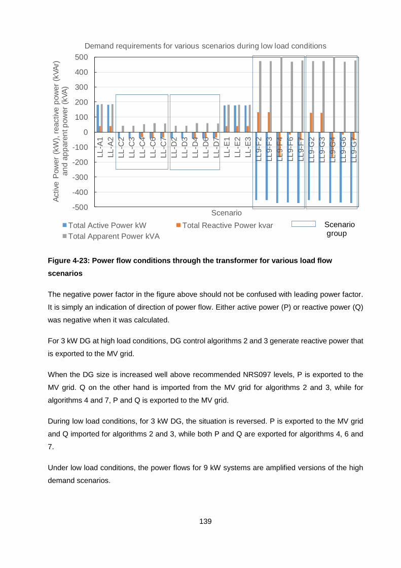
139
Figure 4-23: Power flow conditions through the transformer for various load flow
scenarios
The negative power factor in the figure above should not be confused with leading power factor.
It is simply an indication of direction of power flow. Either active power (P) or reactive power (Q)
was negative when it was calculated.
For 3 kW DG at high load conditions, DG control algorithms 2 and 3 generate reactive power that
is exported to the MV grid.
When the DG size is increased well above recommended NRS097 levels, P is exported to the
MV grid. Q on the other hand is imported from the MV grid for algorithms 2 and 3, while for
algorithms 4 and 7, P and Q is exported to the MV grid.
During low load conditions, for 3 kW DG, the situation is reversed. P is exported to the MV grid
and Q imported for algorithms 2 and 3, while both P and Q are exported for algorithms 4, 6 and
7.
Under low load conditions, the power flows for 9 kW systems are amplified versions of the high
demand scenarios.
-500
-400
-300
-200
-100
0
100
200
300
400
500
LL
-A1
LL
-A2
LL
-C2
LL
-C3
LL
-C4
LL
-C6
LL
-C7
LL
-D2
LL
-D3
LL
-D4
LL
-D6
LL
-D7
LL
-E1
LL
-E2
LL
-E3
LL
9-F
2
LL
9-F
3
LL
9-F
4
LL
9-F
6
LL
9-F
7
LL
9-G
2
LL
9-G
3
LL
9-G
4
LL
9-G
6
LL
9-G
7
Active
Pow
er
(kW
), r
eactive
pow
er
(kVA
r)an
d a
pp
are
nt p
ow
er
(kVA
)
Scenario
Demand requirements for various scenarios during low load conditions
Total Active Power kW Total Reactive Power kvar
Total Apparent Power kVA
Scenariogroup

140
High levels of exported power to the MV grid will be in violation with NRS097, which determines
that only 15% of power should flow in the reverse direction for MV feeders.
Chapter summary
In this chapter, the findings from the load profile simulation indicate that changes to load profiles
can be studied and ADMD’s calculated when circumstances change. The changes to ADMD, load
factor and coincidence were studied when energy efficiency and DG is implemented. This aids
the understanding of how design assumptions change when circumstances change on the
distribution networks for which it was not designed.
These assumptions can be reviewed by a utility in a controlled environment where consumers
approach the utility before they add DG to the network.
The load flow analysis in this chapter demonstrates that utilities can expect degraded
performance of their LV networks when consumers deploy DG in an uncontrolled manner. When
consumers simply add DG without consultation with the utility, the risk exists that voltages may
rise along LV feeders above 1.1 p.u. or cables may be overloaded.

141
Chapter 5 Conclusion
Load profile modelling conclusion
The research and simulations showed that the impact of appliance type and rating changes to a
load profile can be demonstrated by an appliance-based modelling approach.
The load factor reduces when distributed generation takes place. Using the load factor and
average energy consumption to calculate or estimate an ADMD may produce incorrect results if
the designer or planner is not aware that DG is present in the system.
Diversity is severely impacted when DG is deployed, especially when high levels of penetration
occurs. This may have an impact on diversity factors used to determine maximum demand or
equipment ratings when considering historical knowledge of diversity factors present in a
distribution system.
In general, energy consumption is reduced when DG is used, but when DG is not used during
peak loading conditions, assumptions about ADMD reductions are not necessarily valid.
Although harmonics may increase, it will not impose a severe contribution to peak demand.
Load flow study conclusion
The load flow studies show that renewables, when used during high loading conditions, even
when penetration levels are low and installed close to a transformer, may cause unbalance and
consequently voltage drop below legal limits at the end of the LV feeder.
Renewables, when implemented during low load conditions at LV level at high penetration levels
and sizes not limited by NRS097 or similar standards, may cause voltage rise at the transformer
to exceed 1.1 p.u. If the deployment of DG is not managed well by a utility, systems may be
deployed by residents that may adversely affect the LV networks feeding them. The deployment
of DG during low demand scenarios may result in a reverse power flow condition. Increased DG
sizes well above NRS097 recommended levels may impact the designed conditions of LV
feeders. Voltage may rise and conductors may be overloaded, resulting in primary LV cable
feeder circuit breakers tripping.
Under low load conditions, when reverse power flow occurs because of solar PV generated, the
Herman-Beta voltage drop method cannot be used when the reverse power-flow ADMD is higher

142
than the normal power flow direction ADMD. New parameters must be calculated because the
ADMD has changed.
Summarized conclusion
3 kW solar PV systems are not a concern under low load conditions for a 5.3 kVA ADMD network.
However, a high penetration of 9 kW solar PV systems in a 5.3 kVA ADMD network will cause
problems. Limiting the PV system sizes to the NRS 097 limits of 4.6 kW in a 1.3 kVA ADMD
network will also cause problems, indicating that limiting a solar PV system to 25% of the
consumer’s potential maximum demand will also not be sufficient. The consumer load profile,
knowledge of the load at low load conditions under DG peak conditions, and designed network
ADMD are important information to consider when adding DG to the network. The study can be
concluded by formulating a formula to check whether problems may be encountered.
Generally, the network will perform satisfactorily if the following condition is met:
𝐴𝐷𝑀𝐷𝑓𝑜𝑟𝑤𝑎𝑟𝑑 ≥ 𝐴𝐷𝑀𝐷𝑟𝑒𝑣𝑒𝑟𝑠𝑒 ... ( 39 )
The ADMD in the reverse power flow direction is a function of the DG size and the demand at the
time. Equation 39 then becomes:
𝐴𝐷𝑀𝐷𝑓𝑜𝑟𝑤𝑎𝑟𝑑 ≥ (𝑃𝑉 𝑠𝑖𝑧𝑒
𝑝𝑜𝑤𝑒𝑟 𝑓𝑎𝑐𝑡𝑜𝑟−𝐷𝑒𝑚𝑎𝑛𝑑𝑆𝑜𝑙𝑎𝑟 𝑚𝑎𝑥) ... ( 40 )
Where
ADMD forward = Designed ADMD when no DG is present (normal power flow
direction from utility source to load), in kVA.
ADMD reverse = Maximum demand in reverse power flow direction divided
by the number of consumers, in kVA.
Demand solar max = Demand recorded at the time of solar maximum (generally
at the time of relative low domestic load conditions), in kVA.
PV Size = Size of PV system installed (AC output), in kW.
Power factor = Power factor of load.

143
Solar PV is only one case of DG where residential systems experience a minimum load
requirement during DG maximum output. Consider the following diagram:
Figure 5-1: 24-hour load profile with reverse power flow as a result of DG
Equation 40 may be generalized further for any form of DG at any time during the day:
𝐴𝐷𝑀𝐷𝑓𝑜𝑟𝑤𝑎𝑟𝑑 ≥ (𝐷𝐺𝑜𝑢𝑡𝑝𝑢𝑡(𝑡)
𝑝𝑜𝑤𝑒𝑟 𝑓𝑎𝑐𝑡𝑜𝑟−𝐷𝑒𝑚𝑎𝑛𝑑𝑡) ... ( 41 )
Where
Demand t = Average demand recorded at time t (total demand at time t
divided by number of consumers), in kVA, prior to any DG
connected.
DG output (t) = DG system output at time t, in kW
If Equation 39, or expanded as Equation 41, yields a true result, the network design will still comply
in both the forward and reverse directions.
-8
-6
-4
-2
0
2
4
6
8
10
-8
-6
-4
-2
0
2
4
6
8
10
00
:30
01
:30
02
:30
03
:30
04
:30
05
:30
06
:30
07
:30
08
:30
09
:30
10
:30
11
:30
12
:30
13
:30
14
:30
15
:30
16
:30
17
:30
18
:30
19
:30
20
:30
21
:30
22
:30
23
:30
DG
ou
tpu
t (kW
)
AD
MD
(kV
A /
ho
use
ho
ld)
Time
Period during which network problems may occur
Period during which reverse ADMD > original designed ADMD Solar PV 9 kW
Conventional profile (No DG) Adjusted profile after DG
( )

144
Review of research questions and associated findings
1) Research Question 4 (RQ4) - What is the relationship between diversity and load factor?
Finding - The Bary curve as indicated during the literature review stage, illustrates the relationship.
The appliance modelling profile simulation study found a relationship that produced a line in the
opposite direction than Bary found.
2) Research Question 5 (RQ5) - How does single-phase injection on the low voltage
network affect the low voltage network’s performance and integrity?
Finding - The effects of DG on unbalance during high load conditions have been demonstrated
through the load flow analysis. DG closer to the transformer under high load conditions at low
penetration may cause unbalance and a voltage drop towards the end of the feeder. During low
load conditions, voltage rise and cable or line overload may be experienced at high penetration
levels when the size of DG is not within NRS 097 recommended limits.
3) Research Question 6 (RQ6) - How does generation from LV and MV
embedded/distributed generation in general affect the network up- and downstream from the point
of generation?
Finding - Embedded generation reduce the real power required from the grid. However, with unity
power factor DG, as is typical with category A1 & A2 inverters, the grid must still produce reactive
power, and as a result, the utility’s power factor will worsen drastically.
4) Research Question 7 (RQ7) - How will ADMD factors be influenced by energy efficiency
and renewable energy generation at low voltage level?
Finding - Load shifting of thermal load can increase the ADMD. Generally, energy efficiency will
reduce the ADMD. Under reverse power flow conditions, the network may be characterized by a
new and higher ADMD at a different time of the day under high DG levels under low load
conditions so that network failures may occur. This will occur only where the utility does not
exercise control over the size of equipment being installed by consumers.
5) Research Question 8 (RQ8) - How are traditional diversity factors affected?
Finding - Diversity factors will decrease or coincidence factors will increase due to a lack of
diversity between remaining type of loads when large loads such as geysers and stoves are
replaced with alternative energy source appliances. The ADMD generally still reduces and the
consumers’ 60 A connections almost becomes an overkill.
6) Research Question 9 (RQ9) - How are system losses affected by load profiles altered by
energy efficiency and reverse power flow due to renewable energy generation?

145
Finding - When the load factor decreases, the losses will decrease through the application of the
load loss factor formula, which is only dependent on the load factor.
The load factor for most of the case studies decreased where large appliances have been
removed, indicating that losses inherently reduced as well, since less current flows.
The load factor also decreased when DG is deployed at the load. The load loss factor will therefore
also decrease, indicating that losses are reduced.
When DG is deployed elsewhere on the grid, the loads will require the same currents to flow
and the same losses will still occur.
7) Research Question 10 - (RQ10) - How are fault levels affected by renewable energy
injection, and what is the impact on protection systems and equipment ratings?
No adverse changes to fault levels were found during simulation. The inverter contribution to fault
current on the primary LV grid is relative small.
However, protection coordination must be reviewed when adding DG to the network.
Review of findings against original hypothesis
The original expected findings compared with findings after completion of the research and
analysis are summarized as follows:
Hypothesis - Energy efficiency generally reduces the system peak and therefore ADMD.
Technical losses would also be reduced.
Finding - The expected finding was confirmed through load profile simulation.
Hypothesis - Load-shifting techniques, when not properly controlled, can increase the ADMD,
especially if the load is associated with thermal storage.
Finding – The analysis conducted by the author for a paper [1] published during the early stages
of the research and analysis confirmed the expected increases in ADMD.

146
Hypothesis - Improving the load factor reduces the diversity between similar load class
consumers.
Finding - The coincidence versus load factor graph indicates that the coincidence factor remained
the same or increased, but hardly decreased for a reduction in load factor. An increasing
coincidence factor is indicative of a loss of diversity, which confirms the initial expected
postulation.
Hypothesis - Reducing the diversity between consumers will impact designed and constructed
networks by increasing the voltage drop experienced by consumers. However, the reduced
energy consumption and demand could mean that the effect is cancelled out or reduced.
Findings:
For a high concentration of reverse power flow there is very little diversity between PV systems.
Resulting excess DG capacity greater than the designed ADMD will cause cables to overload.
Voltage drop is not the concern, but rather voltage rise and equipment loading.
A reduction in energy consumption combined with large PV systems during low load conditions
may still cause overloading of conductors and voltage rise nearing upper limits.
A high penetration of PV is not likely, although localized cases may occur, such as a developer
installing PV in a housing complex for all the residential units.
PV systems designed at NRS097 recommended upper limits may still cause problems where the
ADMD is lower than the excess DG capacity. The key factor is to not only consider NRS 097 limits
in isolation, but also the localized network ADMD and the customer profiles.
Hypothesis - Uncontrolled solar PV injection into the network may cause network unbalance,
which will affect voltage drop of designed and constructed networks. LV networks is designed for
a diversified power flow in one direction.
Finding - Network unbalance can occur with only one distributed generator connected close to
the transformer. DG located closer to the transformer have a larger effect on unbalance and
voltage drop at the end of the feeder, than DG located closer to the end of the feeder.

147
Hypothesis - A reverse power flow in a high penetration solar PV network producing excess
energy during solar peak will exceed the power a LV feeder can handle due to a lack of diversity
during reverse power flow.
Finding - The load flow studies for 9 kW solar PV systems illustrated that a network’s performance
may be adversely affected when DG sizes are not limited by a utility.

148
Chapter 6 Recommendation for further study / work
It is recommended that the following future work be considered:
Simulation model
Improvements to the Matlab model can be made as follows:
• Appliance modelling in this study assumed a fixed usage duration. The model may be
improved by varying the usage duration.
• The list of appliances is fixed in the model. Make the list of appliances editable to allow
appliances to be added or removed.
• Ten household types are predefined in the model. Make the list of household types
editable. This can perhaps be combined with further classification using the Living
Standard Measure (LSM).
• Expand the appliance model further by modelling duty cycle in more detail, e.g.
refrigerators.
• The model does not group household nodes into transformer zones, MV feeder zones,
substation zones or HV feeder zones. Amend the model to allow higher level network
grouping of loads.
• The model indicated what is to be expected at higher penetration levels of DG. Networks
with high penetration should be considered for detailed measurement and analysis to
compare the modelled results with actual measurements.
• Appliance modelling can be further expanded to not only take active power into
consideration with a fixed power factor, but to also allow for the reactive power
consumption to be modelled.
• The model assumes the same size DG for all households where DG is randomly
introduced. The model can be expanded by allowing variable DG size, as well as variable
type (e.g. solar PV and micro wind turbines).
• NRS097 limits can be introduced in the model for further studies. The primary aim of this
dissertation was to observe the impact of DG when no limitations were in place.

149
Reactive power and power factor
• The economic viability of domestic inverters with reactive power generation capability
should be investigated. Voltage profiles in general may be improved by generation of
reactive power by the consumer. This should also reduce losses on the utility’s side.
• With power factor as viewed from a utility reducing considerably as larger quantities of DG
is implemented, a case may be made for billing kVAh instead of kWh, or utilities will have
to install meters capable of recording both kWh and kvarh consumed and generated.
• The contribution of reactive power to losses was not studied. This should be a study on
its own.
Protection
• LV circuit breaker coordination for reverse feed conditions can be investigated.
Thermal cycling
• The Matlab model did not take thermal cycling of transformers, cables and overhead lines
into consideration. With the variability of DG introduced into the distribution networks, it is
proposed that the thermal cycling of network elements be studied further to obtain a better
understanding of random behaviour of loads with a view on dynamic capacity ratings.

150
REFERENCES
[1] J. A. Alberts and J. A. de Kock, “The impact of small scale embedded generation on
existing networks,” in Proceedings of the 64th AMEU Convention, 2014, pp. 56–60.
[2] E. Bunge and M. du Preez, “Eskom methodology for network master plans and network
development plans.” Eskom, DGL 34-431, 2007.
[3] SANS (South African National Standards), “Electricity distribution — Guidelines for the
provision of electricity distribution networks in residential areas, Part 1 : Planning and
design of distribution networks,” Pretoria: SABS, Standards Division, NRS 034-1 (SANS
507-1), 2007.
[4] NERSA, “System adequacy outook,” Pretoria: NERSA, 2016.
[5] Eskom, “Tariffs & Charges 2016/17,” Eskom, 2016.
[6] H. L. Willis, Power distribution planning reference book, 2nd Ed. New York: Marcel Dekker,
2004, pp. 875–879.
[7] H. L. Willis, Spatial electric load forecasting, 2nd Ed. New York: Marcel Dekker, 2002, pp.
1–127.
[8] CSIR, Guidelines for human settlement planning and design, vol. 2. Pretoria: CSIR,
Building and Construction Technology, 2005.
[9] K. D. Mistry and R. Roy, “Enhancement of loading capacity of distribution system through
distributed generator placement considering techno-economic benefits with load growth,”
International Journal of Electrical Power & Energy Systems, vol. 54, 2014, pp. 505–515.
[10] I. A. Ferguson, “Distribution standard part 1: Planning guidelines, Section 23: Book –
Electrification load forecasting,” Eskom, SCSASAAB0, 2000.
[11] D. McQueen, M. McQueen, P. Hyland, and S. Watson, “Simulation of power quality in
residential electricity networks,” in Proceedings of the 2003 International Renewable
Energies and Power Quality Conference, 2003, pp. 620–627.
[12] J. Boggis, “Diversity, bias and balance,” Distribution of Electricity, 1953, pp. 357–362.
[13] C. Bary, “Coincidence-factor reationships of electric-service-load characteristics,”

151
Transactions of the American Institute of Electrical Engineers, vol. 64, no. 9, 1945, pp.
623–629.
[14] C. T. Gaunt, R. Herman, and H. Kadada, “Design parameters for LV feeders to meet
regulatory limits of voltage magnitude,” in 21st International Conference on Electricity
Distribution, 2011, pp. ?.
[15] H. W. Beaty and D. G. Fink, Standard Handbook for Electrical Engineers, 15th Ed. McGraw
Hill, 2007.
[16] G. Celli, C. T. Gaunt, R. Herman and S. Mocci, “MV and LV distribution feeder design using
probabilistic approaches to load and DG Introduction,” CIRED Tutorial 5, 2011.
[17] Eskom, “Distribution standard part 1: Planning guidelines, Section 44: Tool - Reticmaster,”
Eskom, SCSASABQ6, 2000.
[18] SANS (South African National Standards), “Cost of supply methodology for application in
the electrical distribution industry,” Pretoria: SABS, Standards Division, NRS 058 (Int),
2000.
[19] United States of America (Department of Defense), “Unified facilities criteria - electrical
engineering preliminary considerations,” UFC 3-501-03N, 2004.
[20] S. Hashe, G. Brand, J. Roesch, and A. Senekal, “Geo-based load forecast guideline
reference,” Eskom, DGL 34-1284, 2007.
[21] I. A. Ferguson and C. T. Gaunt, “LV network sizing in electrification projects — replacing a
deterministic method with a probablistic method,” 17th International Conference on
Electricity Distribution, 2003, pp. ?.
[22] Y. Li, “Statistical and probabilistic models for smart electricity distribution networks,” Ph.D.
thesis, Department Electrical and Computer Engineering, Curtin University, Curtin,
Australia, 2013.
[23] NERSA, “The South African grid code: the network code,” Pretoria: NERSA, 2010.
[24] NERSA, “The South African grid code: the transmission tariff code,” Pretoria: NERSA,
2010.
[25] NERSA, “South African distribution code: network code,” Pretoria: NERSA, 2014.

152
[26] NERSA, “Grid connection code for renewable power plants (RPPs) connected to the
electricity transmission system (TS) or the distribution system (DS) in South Africa,”
Pretoria: NERSA, 2014.
[27] C. T. Gaunt, R. Herman, M. Dekenah, R. L. Sellick, and S. W. Heunis, “Data collection,
load modelling and probabilistic analysis for LV domestic electrification,” 15th International
Conference on Electricity Distribution, 1999, pp. ?.
[28] E. Kreyzig, Advanced Engineering Mathematics, 10th Ed. Wiley, 2005.
[29] SANS (South African National Standards), “Grid interconnection of embedded generation,
Part 2 : Small-scale embedded generation, Section 1 : Utility interface,” SABS Standards
Division, Pretoria: SABS, Standards Division, NRS 097-2-1, 2010.
[30] SANS (South African National Standards), “Grid interconnection of embedded generation,
Part 2: Small-scale embedded generation, Section 3: Simplified utility connection criteria
for low-voltage connected generators,” Pretoria: SABS, Standards Division, NRS 097-2-3,
2014.
[31] SANS (South African National Standards), “The wiring of premises, Part 1: low-voltage
installations,” Pretoria: SABS, Standards Division, SANS 10142-1, 2012.
[32] M. van Harte, “Network planning reliability guideline,” Eskom, DGL 34-350, 2007.
[33] SANS (South African National Standards), “Energy efficiency in buildings,” SABS
Standards Division, Pretoria: SABS, Standards Division, SANS 204, 2011.
[34] M. Vandenbergh et al., “Prioritisation of technical solutions available for the integration of
PV into the distribution grid,” DERlab (www.pvgrid.eu), D3.1, 2013.
[35] K. Balamurugan, D. Srinivasan, and T. Reindl, “Impact of Distributed Generation on Power
Distribution Systems,” Energy Procedia, vol. 25, 2012, pp. 93–100.
[36] R. Arghandeh, A. Onen, J. Jung, and R. P. Broadwater, “Harmonic interactions of multiple
distributed energy resources in power distribution networks,” Electric Power Systems
Research, vol. 105, 2013, pp. 124–133.
[37] J. Bloem, “Power quality and utilisation guide: Distributed generation and renewables,”
KEMA Nederland B.V, 8.3.1, 2007.
[38] M. Farhoodnea, A. Mohamed, H. Shareef, and H. Zayandehroodi, “Power quality impacts

153
of high-penetration electric vehicle stations and renewable energy-based generators on
power distribution systems,” Measurement, vol. 46, no. 8, 2013, pp. 2423–2434.
[39] A. F. S. Sarabia, “Impact of distributed generation on distribution system,” Masters
dissertation, Faculty of Engineering, Science and Medicine, Aalborg University, Aalborg,
Denmark, 2011.
[40] D. Q. Hung, N. Mithulananthan, and R. C. Bansal, “Integration of PV and BES units in
commercial distribution systems considering energy loss and voltage stability,” Applied
Energy, vol. 113, 2014, pp. 1162–1170.
[41] G. Lacey, G. Putrus, E. Bentley, D. Johnston, S. Walker, and T. Jiang, “A Modelling Tool
to Investigate the Effect of Electric Vehicle Charging on Low Voltage Networks,” in 27th
International Electric Vehicle Symposium, 2013.
[42] A. Di Gangi and A. Orioli, “Load mismatch of grid-connected photovoltaic systems: Review
of the effects and analysis in an urban context,” Renewable and Sustainable Energy
Reviews, vol. 21, 2013, pp. 13–28.

154
Appendices
Appendix A: Appliance model load simulation tool: User Interface
Overview
7.1.1 User interface outline
The user interface consists of four main tabs, each with sub-tabs as follows:
• Profile
o Main UI
o Total Load Profiles
o Graphs
o Study cases
o Sorted study case
• Hourly tables
o Appliance Present
o Appliance Active
o Appliance load (kW)
o Appliance “On” Duration (Minutes)
• Minute tables
o Households
o Appliance_Probability_On
o Appliance_Minute_Start
o Appliance_Minute_On
o Appliance_Load_Minute
o Profile per household (T)
• EE / DSM / Green measures
o Appliance Modify
7.1.2 Application usage
The main focus of the application is to calculate load profiles from input parameters. Input
parameters consist of the number of households, as well as a few tables that were originally
generated in Excel and imported into Matlab and stored in a variable file.

155
For every 24-hour load profile calculated, the application also calculates an adjustment profile,
which is based on parameters set on the EE / DSM / Green Measures main tab.
Every calculation’s load profile, adjusted load profile and profile parameters are added to a study
case database. It is also possible to set up a few calculations to run at a time to append the study
case database faster. This is performed on the Study case sub-tab of the main Profile tab.
Histograms and scatter plots are provided to display the study case database data.
Table views are provided of the imported Excel vectors and matrices, which can be edited in
Matlab, as well as the calculated matrices (which cannot be edited). The calculated matrices are
mostly displayed for diagnostic purposes. The calculated matrices displayed are only for the last
profile calculated. The displayed matrices are scrollable for all the households, allowing viewing
each household’s calculated profile, as well as how it was derived. The Excel imported vectors
and matrices remain the same throughout, unless edited, while the calculated matrices are re-
calculated for every calculation. This is mainly due to the random numbers generated for
probability that an appliance is on, the household type a household belongs to as well as the
starting minute within an hour for an appliance.
In study case mode, the detail tables are only stored for the last calculation executed. The case
study variable file otherwise would have become very large. It has been observed that variable
files in the order of 500MB generally can be handled, but larger files tend to become corrupt (in
the order of 200 case studies depending on the number of households selected). The case study
database was built up after many executions of the program and data copied to Excel where the
main parameters were analyzed. 744 case studies were transferred to Excel for further analysis.
Only the calculated parameters (ADMD, load factor, coincidence, diversity, kWh / day etc.) as
well as the state of the appliances were transferred to Excel. The stored profiles are only available
for the last 443 study cases (543 MB) since the previous corrupted case file.
The main UI and the various routines it calls send feedback messages to the Matlab command
window. This was mainly built in for diagnostic purposes or to know what it is busy with during
lengthy calculations. Selected messages are also displayed within the main UI.
7.1.3 Application routines
The following Matlab files form part of this application:

156
Table 7-1: Matlab application file list
No. File name Description
1. USER INTERFACE (UI)
1.1 LoadProfileSimUI.m Main UI file
2. PROFILE AND STUDY CASE CALCULATIONS
2.1 Load_profile_calcuations.m Calculates the load profile. Called from the main UI
by either the Calculate or the Generate study
cases buttons. Generates a study case each time
it is executed and calls the AdjustProfile routine
2.2 ExtractParameters.m Extracts the parameters for the study case and is
called from the Load_Profiles_Calculation routine
2.3 CreateStudycase.m Creates the study case and is called from the
Load_Profiles_Calculation routine
2.4 AdjustProfile.m This makes the adjustments to the load profile
based on green measures selected. This is called
by the Load_Profile_Calculations routine, but can
also be called directly from the main UI through the
Adjust Load Profile button on the EE / DSM / Green
measures tab. When called from the UI, it does not
add to the study cases.
2.5 GeneratePVprofile.m This generates a solar PV "parabolic" simulated
profile with no shade. This is called by the
AdjustProfile routine. It can also be called from the
main UI. When called from the main UI, it only
calculates the PV curve and plots it.
3. GRAPH PLOTTING CUSTOMIZED ROUTINES
3.1 PlotTimeArray.m This is a customized graph plotting function that
can plot a time-based graph on either hourly or
minute based X-axis and can scale the X and Y
axis based on variable data

157
No. File name Description
3.2 PlotHistogram.m This plots a customized histogram – at this stage
it only plots the current distribution at peak time
across the set of households.
3.3 PlotScatter.m This plots a customized scatter plot of study case
parameters, e.g. ADMD vs number of households
4. IMPORT AND EXPORT (FROM AND TO EXCEL)
4.1 ReadDataFromExcel.m This reads the Bottom-up load profile modelling
Excel spreadsheet. It was only used once to create
the ExcelVariables.mat file. Thereafter the
parameters are edited in the main UI and stored in
the ExcelVariables.mat file.
4.2 WriteData2Excel.m Not really used, but can be used to export tables
back to Excel. It creates a different file named
Test.xlsx and does not overwrite data in the main
Excel parameters file.
4.3 ReadReferenceProfilefromExcel.m This reads 31 reference profile days from a load
profile spreadsheet (already processed to isolate
the 31 days’ one-minute profiles). Creates the
ReferenceProfile.mat variable set. The Reference
Profile is used to compare against the calculated
profile.
5. STORED VARIABLES
5.1 ExcelVariables.mat Stores the original few tables imported from Excel,
and is updated when modified in the main UI. This
update is not automatic.
5.2 ProfileVariables.mat Stores the calculated profile variables. The
application automatically generates a backup
profile data set as well, appended by the number
of study cases in it, so that a manual replacement
of a corrupted profile variable set can be made.

158
No. File name Description
5.3 ReferenceProfile.mat Creates the ReferenceProfile.mat variable set.
The Reference Profile is used to compare against
the calculated profile. Contains 31 reference
profile days from a load profile spreadsheet
downloaded from meters and processed to isolate
the 31 days’ 1-minute profiles.
5.4 CaseProfileVariables.mat Stores the study case database as well as
calculated profiles for each study case. The
application automatically generates a backup
profile data set as well, appended by the number
of study cases in it, so that a manual replacement
of a corrupted profile variable set can be made.
Study case parameters can be manually copied
from the main UI to Excel where further analysis
can take place.
Profile tab: The main user interface (UI) sub-tab
7.2.1 Main components
The main user interface screen has the following components:
• Tabs and sub-tabs
• Graph screen displaying measurement reference and simulated load profile curves
• Buttons for various functions
• Parameter display
• Scroll bars to select different reference profile curves and stored case-file profile curves.
• Message display

159
Figure 7-1: Main User Interface (UI) screen / start-up screen
The application displays graphs of the last profile calculated. The following graphs are displayed:
• Calculated composite load profile for a group of consumers: Black curve
• Reference load profile: Magenta curve, from actual, one-minute measured data
• Calculated domestic load profile: Blue curve (the main focus curve for the baseline)
• Calculated adjusted domestic load profile: Red curve (the main focus curve for the
adjusted profile)
• Calculated non-domestic load profile: Green curve.
When the application starts up, the last profile previously calculated and stored in the
ProfileVariables.mat file is displayed. In the event that it is the first profile to calculate, it calculates
a profile for 50 households by default, and an adjusted profile for 10% PV penetration with 1.5kW
solar PV systems. No solar geysers or gas stoves are applied to the initial start-up adjustment
profile. 50 households were chosen so that the program does not take too long to load. Calculating
e.g. 1500 households take a considerable time (> 5 minutes).
Calculated profiles are stored in the variable files ExcelVariables.mat and ProfileVariables.mat.
Reference profiles are stored in the variable file ReferenceProfile.mat, while case study data are
stored in CaseProfileVariables.mat.
The ExcelVariables.mat and ReferenceVariables.mat files must exist. Any of these files do not
exist, it is imported from Excel. If the Excel files do not exist, the program cannot function. A

160
default reference profile is selected (Profile 6 of 31). Thereafter, the user can change the
reference profile viewed from a selection of 31 consecutive day profiles. If the ProfileVariables.mat
file does not exist, the program creates it as well as the CaseProfileVariable.mat file and initializes
it with default values required to perform the first calculation.
7.2.2 Button functions
The Main UI screen contains the following buttons with functions as described:
• Calculate: This button calls the profile calculation routine which calculates a profile as
well as an adjusted profile based on the “number of households” input parameter specified
on the main UI screen. The adjusted profile takes effects such as solar PV, replacement
of appliances with more energy efficient appliances etc. into consideration, while the
normal profile is calculated without any form of intervention.
• Quit: This quits the application
• Write to Excel: This button calls a routine to write out the various matrices to Excel. It was
used for diagnostic purposes.
• Read From Excel: This button calls a routine which reads the Excel variables required
initially, and stores the results in the ExcelVariables.mat file.
• Clear Variables: This button calls a routine which clears the variables from memory.
• Save Variables: This button saves the variables to ProfileVariables.mat.
7.2.3 Input variables
The only input variable on this screen at this stage is the number of households. It is best to keep
the input value below 1500. A large household quantity takes a considerable amount of time to
calculate. Once the value is edited, a feedback message indicates that a calculation is required.
Profile tab: Total load profile data
The Total load profile data sub-tab displays the total composite, domestic and non-domestic load
profile matrix data calculated by the application. Only the last profile calculated is displayed. This
data corresponds to the graph plotted on the Main UI sub-tab.

161
Figure 7-2: One-minute calculated profile screen
The profiles display 1440 columns, one for every minute in a 24-hour day. Column references for
the various hours of the day are listed in Table 2.2-1:
Table 7-2: Column headings related to time of the day
Time Column Time Column Time Column Time Column
01:00 60 07:00 420 13:00 780 19:00 1140
02:00 120 08:00 480 14:00 840 20:00 1200
03:00 180 09:00 540 15:00 900 21:00 1260
04:00 240 10:00 600 16:00 960 22:00 1320
05:00 300 11:00 660 17:00 1020 23:00 1380
06:00 360 12:00 720 18:00 1080 24:00 1440
Total Non-Domestic load profile (kW values) for each minute of the day

162
Profile tab: Graphs sub-tab
The Graphs sub-tab of the Profile main tab displays a histogram as well as scatter plots of the
study case database.
Figure 7-3: Graphs screen
Histograms, scatter plots and two scroll bars are displayed.
The scroll bar to the left is used to select the study case number for the histogram. Text messages
display the time of the day (in minutes6) the peak was recorded for the Conventional profile (i.e.
the profile without any interventions, indicated in blue) as well as the adjusted profile (after “green”
interventions, indicated in red). The scroll bar to the right is used to scale the x-axis of the scatter
plots.
The histogram displays the current at the time of maximum demand. The time of the maximum
demand for the two Conventional and Adjusted profiles may be different. It especially becomes
clear when a new peak occurs as a result of excess energy generated by a solar PV system.
6 The time is displayed in minutes counting from midnight to ensure that the corresponding column in the data tables can be located easily.

163
Due to limitations by Matlab for the legend, scatter plots were re-generated in Excel from the
study case database. The Conventional profile data is displayed in grey dots on the scatter plots,
while PV, solar geysers and gas stoves, and the respective combinations, produced different
colours using the status indicators in the study case database as RGB bit indicators.
A curve fitting algorithm was used to plot a trend. The conventional load profile trend is displayed
using blue while the adjusted profile trend is displayed using red.
Profile tab: Study cases
The Study cases sub-tab shows the study case data. The study case data displays the study case
number, the number of households, the profile parameters for a profile without any energy
efficiency applied, as well as a modified profile with green measures active. Record of each
appliance’s status (whether modified or not) is also recorded, as well as PV penetration level and
size.
Three input boxes allow the user to select a lower and upper limit for household quantities to
generate study cases, as well as the number of simulations per household quantity. The
household quantities are increased in steps as follows:
• 0-199: steps of 20
• 200-499: steps of 50
• 500-999: steps of 100
• ≥1000: steps of 1000.

164
Figure 7-4: Study cases sub-tab screen
Profile tab: Sorted study case
This display is similar to the Study cases sub-tab with the exception that study cases cannot be
generated from this tab. It simply shows the study cases sorted according to the number of
households.
Figure 7-5: Sorted study cases sub-tab screen

165
Hourly tables
7.7.1 Appliance Present
The Appliance Present sub-tab lists two table views: one for the non-domestic load, and one for
the domestic load. A check-box is provided to select whether the non-domestic data as listed in
the table view should be used, or as built-in. When selected, the table-view is used. When it is
not selected, the built-in parameters as obtained from town planners are used.
The Appliance Present sub-tab displays the appliance present per type of household. Household
types are defined in table 0.
Figure 7-6: Appliance Present sub-tab screen
These two tables can be edited.

166
The built-in data was obtained from a town-planner, and is as follows:
Type of installation or
parameter
Criteria
Household Size 3.2 persons per household
Population (persons) Number of Households multiplied by Household Size
Creches 1 per 5 000 persons
Primary Schools 1 per 3 300 persons
Secondary Schools 1 per 6 600 persons
Clinics 1 per 5 000 persons
Hospitals 1 per 10 000 persons
Libraries 1 per 25 000 persons
Community Centers 1 per 22 000 persons
Churches 1 per 2 000 persons
Municipal Offices 1 per 50 000 persons
Police Stations 1 per 25 000 persons
Fire Stations 1 per 60 000 persons
Retail Floor Area 1 m2 per 2 persons - not according to any guideline. Based on
actual projects
Business Floor Area 1 m2 per 1.25 persons - not according to any guideline. Based
on actual projects

167
7.7.2 Appliance Active
The Appliance Active sub-tab indicates the appliances which can be switched on during certain
times of the day. The table lists 24 hour slots horizontally. Values represent a value between 0
and 1 which effectively doubles as a scaling factor of the full load. Values were initially chosen as
either 0 or 1, but modified later to be any value between 0 and 1.
Values are shown for non-domestic as well as domestic load. These two tables can be edited.
Figure 7-7: Appliance Active sub-tab screen

168
7.7.3 Appliance load (kW)
The appliance load in kW is shown for domestic appliances and non-domestic load classes.
These values can be edited.
Figure 7-8: Appliance load sub-tab screen

169
7.7.4 Appliance “On” Duration (Minutes)
The appliance load duration, in minutes, from the moment it is switched on, is displayed for non-
domestic load classes and domestic appliances. The duration of non-domestic load classes is by
default 60 minutes. Random starting minutes are not generated for load with a 60-minute or longer
duration per hour. In such a case the load starts at minute and continues for 60 minutes.
These two tables can be edited.
Figure 7-9: Appliance "On" duration sub-tab screen

170
MINUTE TABLES
7.8.1 Households
The Households sub-tab shows the table after the random values of household types it belongs
to, has been generated. The table is generated for every profile or case study calculated. The
table cannot be edited.
Figure 7-10: Households sub-tab screen

171
7.8.2 Appliance_Probability_On
The Appliance_Probability_On sub-tab shows the matrix once random numbers have been
generated. The random numbers are generated between 0 and 100, then divided by 100 and
rounded to the nearest integer. Either a 0 or 1 will be obtained. This table cannot be edited. The
random numbers are generated for every profile calculation or study case. The user can scroll
through each household’s table.
Figure 7-11: Appliance_Probability_On sub-tab screen
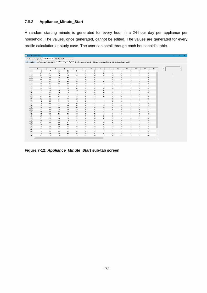
172
7.8.3 Appliance_Minute_Start
A random starting minute is generated for every hour in a 24-hour day per appliance per
household. The values, once generated, cannot be edited. The values are generated for every
profile calculation or study case. The user can scroll through each household’s table.
Figure 7-12: Appliance_Minute_Start sub-tab screen

173
7.8.4 Appliance_Minute_On
The Appliance_Minute_On sub-tab shows the result of the conversion from hourly tables to a
minute table. This table cannot be edited, and is recalculated for every profile calculation or study
case. The user can scroll through each household’s table. The table has 1440 columns
horizontally, representing 60 minutes per hour for 24 hours.
Figure 7-13: Appliance_Minute_On sub-tab screen

174
7.8.5 Appliance_Load_Minute
The Appliance_Load_Minute is simply the product of the Appliance_Minute_On matrix with the
Appliance_Load vector. The values cannot be edited by the user, and are recalculated for every
profile or study case calculation. The user can scroll through each household’s table. The table
has 1440 columns horizontally, representing 60 minutes per hour for 24 hours.
Figure 7-14: Appliance_Load_Minute sub-tab screen
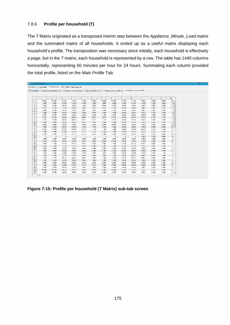
175
7.8.6 Profile per household (T)
The T Matrix originated as a transposed interim step between the Appliance_Minute_Load matrix
and the summated matrix of all households. It ended up as a useful matrix displaying each
household’s profile. The transposition was necessary since initially, each household is effectively
a page, but in the T matrix, each household is represented by a row. The table has 1440 columns
horizontally, representing 60 minutes per hour for 24 hours. Summating each column provided
the total profile, listed on the Main Profile Tab.
Figure 7-15: Profile per household (T Matrix) sub-tab screen

176
EE/DSM Green measures
The Appliance Modify sub-tab allows the user to adjust appliance loads. A load can only be edited
if it has been selected. A check box exists to include or omit PV. The PV curve is adjusted by
changing the size of the PV. The display shows only integer values, although the actual value
entered, e.g. 1.5 will be used (will show as 2 after entering the value of 1.5). The PV penetration
level is entered as a value without a percentage sign (e.g. to enter 20%, enter the value 20).
Figure 7-16: Appliance modify sub-tab screen