i

Impact of Financial variables on the

production efficiency of Pangasius farms

in An Giang province, Vietnam

Bui Le Thai Hanh

FSK-3911: Master Thesis in Fisheries and Aquaculture

Management and Economics

(30 ECTS)

The Norwegian College of Fishery Science

University of Tromso, Norway

&

Nha Trang University, Vietnam

May 2009

i

ACKNOWLEDGMENTS

I would like to express special appreciation to my supervisor, Professor Terje Vassdal who

I have learned a lot from his guidance, useful recommendations and valuable comments.

I would like to thank my mother, Dr Le Thi Men, and her undergraduate students who

helped me to collect the data during my field trip in An Giang province.

I am grateful to the NOMA FAME programme and NORAD for sponsoring my study and

stay in Nha Trang city.

This thesis is dedicated to my parents, parents in-law and my husband who always love,

support, and concern me during my studying in Nha Trang. Especially, thank to my unborn

baby, who accompanied and encouraged me a lot in working hard last 3 months!

Nha Trang, May 15th 2009

Bui Le Thai Hanh

ii

CONTENTS

CHAPTER 1: INTRODUCTION ....................................................................................... 1

OBJECTIVES OF THE THESIS: ....................................................................................... 2

HYPOTHESES ..................................................................................................................... 2

PROCEDURE AND METHODOLOGY: ............................................................................ 3

EXPECTED RESULTS: ....................................................................................................... 3

ORGANIZATION OF THE THESIS: ................................................................................. 3

CHAPTER 2: LITERATURE REVIEW ........................................................................... 5

2.1. Basic efficiency concepts: ............................................................................................. 5

2.2. Techniques of efficiency measurement........................................................................ 5

2.3. The DEA approach to efficiency measurement. ......................................................... 7

2.4. DEA applications in Aquaculture ................................................................................ 9

2.5. The relationship of Financial variables and technical efficiency: .......................... 10

CHAPTER 3: MODEL DEVELOPMENT AND DATA ............................................... 15

3.1. METHODOLOGY ...................................................................................................... 15

3.1.1. STEP 1: Efficiency measurement......................................................................... 15

3.1.2: STEP 2: Sources of Technical Efficiency............................................................ 19

3.2. DATA DESCRIPTION ............................................................................................... 21

CHAPTER 4: RESULTS ................................................................................................... 25

4.1. Efficiency Scores ......................................................................................................... 25

4.1.1. Technical eficiency scores by region ................................................................... 27

4.1.2. Efficiency – Pond size relationship ..................................................................... 31

4.2. Technical Efficiency and Farm-Specific Factors ....................................................... 35

4.2.1. Test for the heteroscedasticity of the errors by the Goldfeld-Quandt test: .... 36

4.2.2. Test for omitted regressors and/or wrong functional form .............................. 37

4.2.3. Ordinary least squares estimation: .................................................................... 38

CHAPTER 5: SUMMARY AND CONCLUSIONS ....................................................... 41

Thesis Summary .................................................................................................................. 41

Results and discussions ....................................................................................................... 41

Conclusion remarks: ........................................................................................................... 43

REFERENCES ................................................................................................................... 45

iii

LIST OF TABLES

Table 3.1: Summary Statistics of Input and Output Variables for Pangasius farms in

AnGiang province .......................................................................................................... 22

Table 3.2: Summary Statistics of data of Farm characteristics Variables for Pangasius

farms in AnGiang province .................................................................................................. 23

Table 4.1: Distribution of Farm Technical and Scale Efficiency Scores: DEA input

orientation ...................................................................................................................... 26

Table 4.2: Technical efficiency and Scale efficiency scores of Region 1 .......................... 28

Table 4.3: Technical efficiency and Scale efficiency scores of Region 2 .......................... 29

Table 4.4: Technical efficiency and Scale efficiency scores of Region 3 .......................... 30

Table 4.5: Mean of technical efficiency scores between regions ...................................... 31

Table 4.6: Efficiency scores of Pangasius farmers according to Pond size less than 4000m2

............................................................................................................................ 32

Table 4.7: Efficiency scores of Pangasius farmers according to Pond size less than 7000m2

............................................................................................................................ 33

Table 4.8: Efficiency scores of Pangasius farmers according to Pond size larger than

7000m2 ............................................................................................................................ 34

Table 4.9: Mean of technical efficiency scores between different group of pond size ... 35

Table 4.10: Parameter estimate and test statistics of Ordinary least squares model ..... 38

iv

ABSTRACT

This research provides the first analysis of the relationship between farm financial exposure

and technical efficiency in the Pangasius farming in An Giang province, in the Mekong

Delta of Vietnam. A nonparametric DEA approach has been applied to estimate technical

and scale efficiency scores of 61 Pangasius farms in An Giang province in the year 2008.

The mean technical efficiencies under assumption of constant returns to scale and variable

returns to scale and scale efficiency were measured to be 0.595, 1.058 and 0.58

respectively. The decomposition of the technical efficiency measure shows that scale

inefficiency is the primary cause of technical inefficiency in the the case of Pangasius

farming as about 92% of the sample Pangasius farms exhibits increasing returns to scale

(IRS). Then, estimated technical efficiency (TE) scores under assumption of variable

returns to scale are used in a regression analysis to investigate the relationship between the

efficiency measures and different farm characteristics, including financial considerations.

Research results suggest that technical efficiency is influenced by investment level of farms

as well as by farm operator‟s experience. The farms are invested more will be more

efficient. The experience measured as the years of operator in farming Pangasius also

suggests that the farmers having more experience may have better decisions in farm

operating and more efficient in using inputs, thus, their farms are more efficient. Technical

efficiency is positively influenced by the debt-to-asset ratio and also by the debt-to-equity

ratio, while no statistically significant relationship is found between technical efficiency

and the bank debt-to asset ratio. The other factors (age and education levels of the houshlod

head) are found to have no effects on the technical efficiency in the sample farms.

Key words: Pangasius farms, Data envelopment analysis, Technical efficiency, Scale

efficiency, Farm debt, Financial variables.

1

CHAPTER 1: INTRODUCTION

Pangasius is one of species of fish that have economic value raised popularly in the

Mekong delta of Vietnam and some countries in Asian (i.e., Cambodia, Thailan, Indonesia).

In recent years, Pangasius is becoming one of the main sectors of the Vietnam aquaculture

and seafood export industry. In ten years, from 1997 to 2006, the farming areas increased

only 7 times, but the annual commercial production of raw fish increased by 36 times from

22,500 to 825,000 metric tones and the volume of exported Pangasius fillets jumped up

more than 40 times, from 7,000 to 286,000 metric tones. In the year 2008, the raw fish

production was 1.65 million M.T and contribute to 657 thousands tons proccessing

products to export to 117 countries and territories and got US$ 1.48 billions of export turn-

over.

In Vietnam, farm-raised Pangasius now are produced in most of provinces in the Mekong

Delta with two species which are Pangasius Bocourti (Basa) and Pangasius Hypophthalmus

(Tra). The water surface areas under Pangasius production totaled about 6,000 hectares at

the end of the year 2008 and created 16 millions jobs relating to the Pangasius industry.

This contributes considerably in the reforms and economic developing in the Mekong Delta

in general. Three provinces of An Giang, Can Tho and Dong Thap are leading culture

regions for Pangasius in the Mekong Delta, accounted for 80% of entire Pangasius

production. An Giang province is the leading with 1.600ha of ponds areas and the

production estimated to the end of October 2008 is 282,000 tons and export turn-over is

about US$ 347 millions.

However, challenges remain. Some problems relating to this industry are out of controlling

in term of zoning and planning from government of different levels, unsustainable

development of this industry relating to environmental impact, crises and fluctuations of

price - production, price competition, conflicts between farmers and producers, and lack of

sustainable financing for farmers.

Nowadays, besides the four countries Thailand, Cambodia, Laos and Vietnam where

Pangasius has raised traditionally, this kind of fish is continued raising in the other

countries and becoming one of the most important rased-fishes in the Southest Asisa.

Assume that the seafood market demand of the world to Pangasius is still large and the

2

imports of aquacultural products are expected to grow, in the long run, the survival of

Vietnam Pangasius may depend firstly on farmer‟s abilities to produce raw fish efficiently.

Pangasius farming requires the huge cultivating and investment costs. Most of Pangasius

farmers have to base their activity on the debt which is mainly bank debt to operate their

farms. Assess to credit has been one of the main constraints to farm operating, restructuring

and technological improvement. Due to this constraint, it may lead to be unsustainable

financing for Pangasius production system and hence decrease the productive efficiency of

Pangasius farming in The Mekong Delta of Vietnam.

OBJECTIVES OF THE THESIS:

The objectives of this research are twofold: to understand the existing Pangasius

farming system in An Giang province, in the Mekong Delta of Vietnam and to investigate

how financial variables affect production efficiency in the case of Pangasius farming.

The specific objectives are:

- to estimate technical and scale efficiency for a selection of Pangasius farms in An

Giang province, to know what are the exhibitions of returns to scale for this sector.

- to examine which factors play an important role in determining farm technical

efficiency.

- and to identify whether there is a relationship between a farm‟s financial variables

and Pangasius production efficiency.

HYPOTHESES

- The variation in technical efficiency scores is considerable among farms with

different input use and technology.

- The variation in technical efficiency scores between the different regions and

different group of pnd sizes.

- There is scale inefficiency of the existing Pangasius farming. This hypothesis is

supported by the statistical follwing information from the Departments of Agriculture and

Rural Development of An Giang province. Pangasius farming areas enlarged and there is

3

farm integration trend, number of bigger farms with farm size 20-40 ha and production of

5,000 to 15,000 metric tones increased in recent time.

- Farm – specific factors are significant factors affecting the efficiency of Pangasius

production.

- There is a positive relationship between a farm‟s technical and scale efficiency and

farm financial variables.

PROCEDURE AND METHODOLOGY:

- Data for conducting research is cross-sectional data (61 samples for the crop in year

2008). Primary data are collected by interviewing directly operators of Pangasius ponds

farms in An Giang province in January 2009. Secondary data are obtained from Department

of Aquaculture of An Giang province.

- A Data Envelopment Analysis (DEA) input-oriented model is employed to measure

pure technical and scale efficiencies of each farm. Resulting estimates of farm technical

efficiency scores are regressed by Ordinary Least Square (OLS) on some financial variables

(Debt - to - asset ratio; Bank debt - to - asset ratio; Debt - to - asset ratio in addition to

other specific factors hypothesized to affect farm efficiency (Investment level of farm, Age

of household head (operator), Education level of household head; household head; in order

to determine the importance of those different factors in explaining efficiency levels.

EXPECTED RESULTS:

- The technical best practice levels of Pangasius production system in An Giang

province of Vietnam.

- The positive effects of financial variables on the production efficiency.

- Policy implications for efficiency improvement on Pangasius farming in Vietnam.

ORGANIZATION OF THE THESIS:

Chapter 2 provides an overview of the existing literature on production efficiency and

measurement, Data Envelopment Analysis (DEA) method to measure the efficiency and

4

applications of DEA in aquaculture. This chapter also present the summay and results

of the recent studies relating to the relationship between financial eposure and

production efficiency.

Chapter 3 desribes methods used to analysis the technical and scale efficiency of

selected farms of Pangasius in An Giang province and to estimate the effects of farm-

specific factors including the farm‟s financial variables on the productive efficiency.

The data used in two steps of analysis also are described fully in this chapter.

Chapter 4 presents results of the thesis.

Chapter 5 includes the summary, discussions and conclusions of the thesis.

5

CHAPTER 2: LITERATURE REVIEW

2.1. Basic efficiency concepts:

Economic efficiency has technical and allocative components. The technical component

refers to the ability to avoid waste, either by producing as much output as technology and

input usage allow or by using as little input as required by technology and output

production. Therefore, the analysis of technical efficiency can have an output-augmenting

orientation or input-conserving orientation.

Koopmans (1951) provided a formal definition of technical efficiency: A producer is

technically efficient if an increase in any output requires a reduction in at least one other

output or an increase in at least one input, and if a reduction in any input requires an

increase in at least one other input or a reduciton in in at least one output. Thus, a

technically inefficiency producer could produce the same output with less of at least one

input or could ues the same inputs to produce more of at least one output.

The preceding definition is replaced by emphasizing its uses with only the information that

is empirically available as in the following definition: (Relative efficiency): A decision

making unit is to be rated as fully (100%) efficiency on the basis of available evidence if

and only if the performances of other DMUs does not show that some of its inputs or

outputs can be improved without worsening some of its other inputs or outputs (Cooper,

Seiford, and Zhu (2004)).

Farrell (1957) introduced a measure of technical efficiency. With an input-conserving

orientation, this measure is defined as one minus the maximum equiproportionare reduction

in all inputs that is feasible with given technology and outputs. With an output-augmenting

orientation, this measure is defined as the maximum radial expansion in all outputs that is

feasible with given technology and inputs. In both orientations, a score of unity means a

firm is technical efficient and a value different from unity indicates the extent of a firm‟s

technical inefficiency.

2.2. Techniques of efficiency measurement

The measurement of productive efficiency is based on deviation of observed performance

from optimal performance located on the efficient frontier. If a firm belongs to the frontier,

it is considered perfectly efficient. In contrast, if a firm is beneath the efficiency frontier,

6

then it is considered inefficient. Because the true frontier is unknown, an empirical

approximation is needed. We estimate a hypothetical frontier that defines the position of

hypothetical most efficinent firms against which positions of actual observations can be

estimated (or calculated). The hypothetical frontier has been estimated using many different

methods over the past 40 years, under different assumptions and implications. The two

principal methods that have been used are data envelopment analysis (DEA) and stochastic

frontier analysis (SFA), which involve mathematical programming and econometric

methods, respectively, according to their assumptions about the functional form of

production (or cost) frontier.

The DEA method is computationally simple and has the advantage that it can be

implemented without knowing the algebraic form of the relationship between outputs and

inputs (i.e., we can estimate the frontier without knowing whether output is a linear,

quadratic, exponential or some other function of inputs).

The second approach (SFA), the contribution of Aigner, Lovell and Schmidt (1977),

simultaneously Meeusen and van den Broeck (1977) and Battese and Corra (1977) is the

introduction of the composed error model, where both stochastic and error components can

be included separately in the error term. This method involves the estimation of a stochastic

function, where besides incorporating the efficiency term into the analysis (as do the

deterministic approaches) also captures the effects of exogenous shocks beyond the control

of the analysed units. When the functional form is specificed then the unknown parameters

of the function need to be estimated using econometric techniques.

The two approaches use different techniques to envelop data in different ways. The

differences between the two approaches can be seen in two essential characteristics and

also the sources of advantages of one approach to the other:

* The econometric is stochastic. This enables it to attempt to distinguish the effects of

noise from those of inefficiency, thereby providing the basis for statistical inference.

* The mathematical programming approach is nonparametric. This enables it to avoid

confounding of effects of misspecification of the functional form (of both technology and

inefficiency) with those of inefficiency.

7

2.3. The DEA approach to efficiency measurement.

The DEA technique uses the linear programming methods to construct a non-parametric

piece-wise surface (or frontier envelopment) for all sample observations, which provides a

yardstick for all DMUs in a sample. This surface is determined by those units that lie on it,

that is the efficient DMUs. Efficiency measures are then calculated relative to this surface.

A unit on the efficient frontier is given a score of 1. Units that do not lie on that surface can

be considered as inefficient and an individual inefficiency score will be calculated for each

one of them, given a score between 0 and 1.

The piece-wise-linear convex hull approach to frontier estimation, proposed by Farrell

(1957), was considered by only a few authors in the two decades following Farrell‟s paper.

The mathematical programming method did not receive wide attention until the paper by

Charnes, Cooper and Rhodes (1978), in which the term Data envelopment analysis (DEA)

was first used. These authors proposed a model that had an input orientation and output

orientation under assumption of constant returns to scale (CRS) and how both models

follows from different fractional programming models.

Since the initial study by Charnes, Cooper and Rhodes, some 2000 articles have appeared

in the literature. Such rapid growth and widespread of DEA is testimony to its strengths and

applicability. At present, DEA actually encompasses a variety of alternative (but related)

approaches to evaluating performance. Some popular extensions of the basic DEA (CRS

and VRS) models so far involve non-discretionary variables, environmental variables,

weights restrictions, super efficiency and bootstrap methods.

The uncontrolled or discretionary variables are an important weakness of model developed

in Charnes, Cooper, and Rhodes (1978). Some variables are outside the control of manager.

Maximization of equi-proportionate contraction should be made by omitting these variables

to obtain more precise efficiency scores. However, in order to get more realistic individual

efficiency scores, one might isolate in some way this type of variable, known as non-

discretionary variables, and their effects on the final performance of the observed units.

Banker and Morey (1986) adapt the mathematical programming treatment of DEA models

to allow a partial analysis of efficiency on the basis of what they initially termed

exogenously and non-exogenously fixed inputs and outputs.

8

Adjusting for the environmetal variables is another extensions of the basic DEA model to

evaluate some factors that could influence the efficiency of a firm, where such factors are

not traditional inputs and are assumed not under the control of the manager. There are a

number of possible approaches to the consideration of environmental variables such as the

“three stages” method proposed by Charnes, Cooper and Rhodes (1981), the possible

method is to include the environmental variable(s) directly into the linear programming

formulation (Ferrier and Lovell (1990). The two-stage approach involving a DEA problem

in the first stage analysis and regressing the efficiency score from the first stage in the

second stage by OLS or Tobit regression is recommended in most cases. Some considerable

advantages of this approach are that both continuous and categorical variables can be easily

accommodated in the second step and hypothesis test to see if the variables have a

significant influence upon efficiencis can be conducted.

The flexibility of the frontier that is constructed using DEA is one of the advantages of this

method. However, this aspect of the method can also create problems, especially when

dealing with small data sets. One can find that the weights assigned to the various input and

output variables are not realistic for some firms since they are too large or too small. A

variety of methods have been proposed to remedy this. Among them, the most relevant are

the Assurance Region (AR) method developed by Thompson, Singleton, Thrall and Smith

(1986) and the Cone-Ratio (CR) method developed by Charnes, Cooper, Wei and Huang

(1989) and Charnes, Cooper, Sun and Huang (1990). The AR approach deals with the

existence of large differences in input/output weights from DMU to another by imposing

additional constraints on the relative magnitude of the weights for some particular

inputs/outputs into the initial DEA model. More general than the AR method, the cone-ratio

approach extends the Charnes, Cooper and Rhodes (1978) model by using constrained

multipliers, which are constrained to belong to closed cones (Murillo-Zamorano, 2004).

Supere fficiency relaten to an DEA model which firms can obtain efficiency scores greater

than one. To calculate a super efficiency score for the i- th firm, the data for the i- th firm is

removed from matrixes of inputs and outputs. Thus, when running the LP, if the i- th firm

was a fully-efficient frontier firm in the original standard DEA model, it may not have an

efficiency score greater than one. This method was originally proposed by Andersen and

Petersen (1993). The problem of infeasibility in that model has been discussed and removed

by Lovell and Rouse (2003), Zhu (2004) and Chen ( 2004).

9

Other extensions to the DEA basic model include the measurement of allocative efficiency

on the basis of price information and the assumption of a behavioural objective such as cost

minimization in Ferrier and Lovell (1990), revenue maximisation in Fare, Grosskopf and

Lovell (1985) or profit maximization in Fare, Grosskopf and Weber (1997); the treatment

of panel data by means of the window analysis developed in Charnes, Clark, Cooper, and

Golany (1985) or the Malmquist index approach of Fare, Grosskopf, Lindgren and Roos

(1994).

2.4. DEA applications in Aquaculture

A great variety of applications of DEA have been conducted in many of studies to

investigate technical, allocative, cost and scale efficiency by applying input and output

oriented models in many different activities in many different contexts in many different

countries. Areas where DEA applied can be mentioned as hospitals, universities, cities,

courts, business firms, banks and others, including the performance of countries, regions,

etc.

There are a number of efficiency studies applying DEA conducted on agricultural sector in

many countries. However, DEA applications on aquaculture are relatively low in

comparison to the other areas.

Sharma et al. (1999) applied a nonparametric DEA technique for multiple outputs to

measure economic or “revenue” efficiency and its technical and allocative components for

a sample of Chinese polyculture fish farms and to derive the optimum stocking densities for

different fish species for Chinese polyculture farms.

Using a weight-restricted DEA technique, Kaliba and Engle (2006) estimate technical,

allocative and cost efficiency of a sample of small- and medium-sized catfish farms in

Chicot County, Arkansas. These authors then regress the cost efficiency score in Tobit

model on operator characteristics, farm practices, and institutional support services to

determine whether these factors lead to a higher level of efficiency. An important finding of

this research is the authors found that higher cost efficiency of catfish farm efficiency in

Chicot County, Arkansas, can be achieved by adjusting inputs used in production to

optimal levels rather than by adjusting the scale of operation.

Also using a two-step procedure, Cinemre et al. (2006) measured the cost efficiency of

trout farms and explored determinants of cost inefficiencies in the Black Sea Region,

10

Turkey. The decomposition of the technical efficiency measure showed that pure technical

inefficiency was the primary cause of technical inefficiency in the sample of trout farms.

Research results also suggested that there were positive relationships between cost

efficiency and pond tenure, farm ownership, experiences of the operators, education level

of the operators, contact with extension services, off-farm income and credit availability

while feeding intensity, pond size, and capital intensity had negative effects on cost

efficiency.

Ferdous Alam, Murshed-e-Jahan, K. (2008) employed DEA technique in evaluating the

resource allocation efficiency of prawn-carp polyculture systems by making use of the data

of 105 farmers of Bangladesh. The results showed that 50 percent of prawn-carp farmers

displayed full technical efficiency whereas only 9 percent were cost efficiency. Technical

and allocative efficiencies showed a positive and negative correlation with pond size,

respectively. Labor, fingerlings and feed were overused while organic and inorganic

fertilizers were underused in general.

In Vietnam, DEA has been applied in several studies in rice farms of the Mekong Delta, the

construction firms, aquaculture processing and food processing companies. So far no study

has been conducted in Vietnam that addressed the aquaculture in general and the Pangasius

farming to evaluate TE, AE, CE and SE.

2.5. The relationship of Financial variables and technical efficiency:

* Theoretical approach:

The seminal work of Modigliani and Miller (1958) on the irrelevance of debt structure to

firm value has prompted numerous continuations in the literature addressing its strong

assumption of perfect capital markets. Under the hypothesis of perfect financial markets,

investment and financing decisions are separable. Thus, a firm should have the same

efficiency level regardless of the way it is capitalized and, consequently, there should not

be any significant statistical impact of leverage on technical efficiency.

Alternatively, economics literature provides arguments for a negative as well as positive

impact of high indebtedness on firm performance. Several hypotheses have been advanced

to explain the positive relationship between efficiency and indebtedness.

The agency theory approach, is based on Jensen and Meckling‟s (1976) agency cost

concept. They defined an agency relationship as a contract under which one or more

11

persons (the principal (s)) engage another person (the agent) to perform some service on

their behalf which involves delegating some decision making authority to the agent. In most

agency relationship, the principal and the agent will incur positive monitoring and bonding

costs and in addition there will be some divergence between the agent‟s decisions and those

decisions which would maximize the welfare of the principal. The agency cost concept

implies that because of the asymmetric information and misaligned incentives between

lenders and borrowers, it requires the monitoring of borrowers by lenders. Lenders may

pass on the monitoring and adverse incentive costs (e.g., high risk taking or unintended use

of loans by the borrower) to the farmers in the form of higher interest rates adjustments,

collateral requirements, etc. (Ellinger and Barry, 1991). As a result, highly indebted farmers

might incur higher costs and, thus, be less technically efficient. Therefore, the agency

theory implies the negative impact of indebtedness on technical efficiency.

The free cash flow concept, developed by Jensen (1986), proposes that issuing large

amounts of debt sets up the required organizational incentives to motivate managers and to

help them overcome normal organizational resistance to retrenchment which the payout of

free cash flow often requires. Debt raise the pressure of managers and serves as an effective

motivating force to make such organizations more efficient. Applied to the agricultural

sector, this concept suggests that farmers with higher debt obligations will be motivated to

improved their efficiency in order to pay their financial obligations. Therefore, the free cash

flow concept implies a positive relationship between technical efficiency and indebtedness.

The third main approach, the credit evaluation concept suggests that lenders will prefer to

finance more efficient farmers because these borrowers are lower credit risks. In addition to

collateral requirements, agricultural bankers often use efficiency variables along with

financial variables in evaluating a farmer's creditworthiness. Thus, the more efficient

farmers might have higher indebtedness because they are selected by banks as good risks.

* Empirical works:

The previous theories are test in the empirical literature by both parametric and

nonparametric approaches that are usual in applications. Following are summarizations and

the main results of recent studies research on the relationship between efficiency and

indebtedness.

12

DEA one stage model was applied in the research of Andreu et al. (2006) which establishes

the cost-efficiency frontier and its variation over time for a sample of 610 farms in Kansas

for ten consecutive years (1995 to 2004) to examine how financially constrained firms

affect cost efficiency and its components, allocatice, technical and scale efficiency. They

employed an output-oriented analysis for model 1 uses DEA in the basic multi-

output/multi-input (7 outputs, 10 inputs) cost minimization problem to estimate TE, AE,SE

and CE. Model 2 and model 3 use DEA in the same context as model 1, except that a

financial constraint is added by the total amount of annual debt and the amount of working

capital for each farm, respectively. Each of the three models were estimated seperately for

each year and then the efficiency scores were compared for each model each year to

investigate if any the two financial constraints imposed are binding. These authors also

compared the efficiency scores each year in terms of farm size and determine if the

difference is statistically significant. The results showed that the farms appear to achieve

the same level of cost efficiency and scale efficiency despite being debt constrained or

working capital constrained in any of the years from 1995 to 2004. However, financially

constrained model 2 and 3 differ in the estimates of technical efficiency and allocative

efficiency. The results for the statistically significant difference in technical efficiency and

allocative efficiency scores between financially-constrained models 2 and 3 and base model

1 suggest that there exists a negative relationship between technical efficiency and the cost

structure of a farm.In contrast, allocative efficiency seems to be positively related to more

indebted farms or those with negative working capital. The results suggest that for farms in

the sample, the financial constraints did not prevent farm from achieving overall cost

efficiency. The authors explained that when farms were constrained by debt or negative

working capital, they compensated the level of technical efficiency and allocative

efficiency to maintain the level of cost efficiency. On the relationships of farm size with

cost and production efficiency measures, there appears a pattern of change for Kansas

farms between 1995 and 2004, where larger farms score higher in the most efficiency

scores except for scale efficiency.

Another group of applications use nonparametric methods to calculate efficiency of firms

in the first stage, and then these values are regressed on various explicative variables. In the

second stage, the tobit regression is used more extensively since it overcome the problems

of data censoring and truncation from DEA analysis. Chavas and Aliber (1993) use

13

information on 545 Wisconsin farms (two output and seven inputs in 1987) and run

different nonparametric models to obtain technical, allocative, scale and scope efficiency

scores. The tobit regression indicate that short-run debt to-asset ratios have no significant

effect on any of the efficiency indexes whereas intermediate and long-run debt to-asset

ratios present positive and significant effects on technical and allocative efficiency. The

results also showed that intermediate and long-run debt to-asset ratios have the effects on

scale efficiency but more complex when such ratios are found to have no significant

relationship with scale efficiency under decreasing returns to scale but have a significant

negative (positive) relationship with scale efficiency under increasing returns to scale.

Those results indicate that there is no statiscal evidence that the financial structure of the

larger farms affects their scale efficiency, however, the financial structure of the smaller

farms affects their ability to attain an efficient scale. In this line, Bezlepina et al. (2004)

examine the impact of debts on managerial performance by using a panel of 144 dairy

farms in the Moscow region over the period 1996-2000. This research considered different

sources of debts (banks, state, suppliers) as well as the different role of debts in poorly and

well performing enterprises. The results suggested that debts, which were mainly the loans

from suppliers in the form of trade credit, were positively related to manageral efficiency.

In addition, a positive effect of debt payables on manageral efficiency was observed. Also

to determine the relationship between farm efficiency and farm debt, Lambert and Bayda

(2005) studied in a panel of 54 North Dakota crop farms in seven years (1995 to 2001).

Farm technical efficiency was found to be influenced by debt structure. A significant

negative relationship was found between technical efficiency and the current debt-to-asset

ratio. The negative relationship supports the agency-cost concept, in which technically

inefficient farmers may not able to generate internal financial resourses to cover operating

expenses so are forced to increase borrowing. At the same time, lenders may impose a

higher proportion of collateral and adverse incentive costs (higher interest rate, servicing

fees) on those producers, therefore, increases their operating costs and lowers their

technical efficiency. The positive relationship between the intermediate debt-to-asset ratio

and technical efficiency supports the credit-evaluation concept, indicating that bankers may

prefer to extend intermediate-term capital to more-efficient farmers. These authors also

examine the effects of farm-specific factors on scale efficiency for farms. Similar to the

results found by Chavas and Aliber, nostatiscally significant relationship existed between

debt structure and scale efficiency for the 205 observations exhibiting decreasing returns to

14

scale. For the 94 observations characterized by increasing returns to scale, there was also no

significant relationship between intermediate- or long-term debt and scale efficiency,

however, current debt-toasset ratio was negatively related to scale efficiency.

Other empirical studies use a stochastic parametric function in the “one stage procedure”

proposed by Battese and Coelli (1995) that include explicative variables to model the error

term and it is estimated by using maximum likelihood techniques. Weill (2001) provided

new empirical evidence on a major corporate governance issue: the relationship between

leverage and corporate performance. The author applied frontier efficiency techniques to

measure performance of medium-sized firms from seven European countries and observed

a positive and significant relationship between leverage and efficiency in four countries

(Belgium, France, Germany, and Norway), while it is negative and significant in Italy and

Spain, and finally not significant in Portugal. He concludes that institutional factors

influence the relationship between leverage and performance. Considering the role of the

access to bank credit on the relationship between leverage and performance, Weill found

that the countries with the lowest access-to-credit-ratio do not have a significantly positive

relationship between leverage and performance. Furthermore, the country with the highest

access-to-credit-ratio, Germany, has the highest significantly positive coefficient for the

Leverage variables. Within agricultural economics, Hadley et al. (2001) contribute to

empirical literature regarding to relationship of financial exposure and farm efficiency by a

study of the England and Wales dairy sector on a panel of 601 dairy farms covering the

production years from 1984 to 1997. A translog distance function is employed representing

one output (revenue) and multiple inputs (rent and land charges, family labour hours, hired

labour hours, feed costs, vet and med costs, crop input costs, misc costs,capital and dairy

hezd size) to study the efficiency. As determinants of technical inefficiency, a number of

variables are incorporated the ratio of total debt to total assets, short-term loans and debt to

total assets and the ratio of long and and medium term loans and debts to total assets were

hypothesised as possibly having a role in explaining differences in levels of technical

efficiency among farms. The results point out that negative estimated coefficients are

related to increases in levels of technical inefficiency, so that increases in the size of the

various debt ratio are all likely to decrease the technical efficiency of farms.

15

CHAPTER 3: MODEL DEVELOPMENT AND DATA

The objective of this research is to examine the production efficiency of Pangasius farms in

Angiang province and to identify whether there is a relationship between a farm's

production efficiency and its financial variables. In the first stage of the analysis, the

technical efficiency and scale efficiency of individual farms is assessed by the data

envelopment (DEA) super-efficiency approach. The second stage consists of a description

of econometric models. A OLS model is employed to assess the influence of selected farm-

specific factors including financial variables on estimated technical efficiency scores.

Finally, data used in the research is described fully in the final part of the chapter.

3.1. METHODOLOGY

3.1.1. STEP 1: Efficiency measurement

The technique of data envelopment analysis (DEA) introduced by Charnes, Cooper and

Rhodes (CCR) (1978) is widely employed for estimation of multiple input, multiple output

production correspondences and the evaluation of the productive efficiency of decision

making units (DMUs). They provided linear programming formulation to measure the

productive efficiency (CCR efficiency) of a DMU relative to a set of referent DMUs.

Banker, Charnes and Cooper (BCC) (1984) showed that the CCR efficiency measure can be

regarded as the product of technical efficiency (BCC efficiency) measure and a scale

efficiency measure.

Technical efficiency is considered in terms of the optimal combination of inputs to achieve

a given level of output (an input-orientation) or the optimal output that can be produced

given a set of inputs (an output-orientation). The envelopment surface of the oriented

models can be either constant returns-to scale (CRS) or variable returns-to-scale (VRS).

Under CRS, the form of the envelopment surface of the constructed production frontier is a

conical hull, while under VRS, it is a convex hull.

The input-oriented models is used for this research since in agriculture, farmers have more

control over their inputs than their outputs. In the case of Pangasius farming in An Giang

province in particular and general, under some certain constraints of financing and the high

16

costs for farming, especially the cost for feed, the choice of the DEA input-oriented models

is make sense.

Suppose we have n DMUs (DMUj : j = 1,2, …, n), which produce s outputs yrj (r = 1,2,…,

s) by utilizing m inputs, xij (I = 1,2,…, m). An input-oriented model which exhibits CRS,

developed by Charnes, Cooper and Rhodes (CCR) (1978) and referred to in the literature as

the CCR model, can be written as

Min θo

n

s.t ∑ λjxij ≤ θoxio, i = 1,2, …, m,

j=1

n

∑ λjyrj ≥ yro r = 1,2, …, s,

j=1

λj ≥ 0, j = 1, …, n, (3.1)

where, xio and yro are, respectively, the ith input and rth output for a DMUo under

evaluation.

Solving that model n times results in optimal values of the objective function and the

elements of intensity variables vector λ for each farm. For the DMUo the optimal value θ*o

measures the maximal proportional input reduction without altering the level of outputs.

The vector λ*

j indicates participation of each considered farm in the construction of the

virtual reference farm that the DMUo is compared with.

Solving the CCR model, the total technical efficiency measure θ*

o (CCR) is obtained by

comparing small scale units with large scale units and vice versa without considering the

economies of scale. This may be inappropriate for all of the farms in the sample. Therefore,

the BCC model, developed by Banker, Charnes and Cooper (BCC) (1984) and called the

input-oriented BCC model, allows for variations in the returns to scale is considered.

The input-oriented VRS model is obtained from the CRS model by adding a convexity

constraint ∑λ = 1 to the CCR model (3.1), , can be written as

Min θo

n

s.t ∑ λjxij ≤ θoxio, i = 1,2, …, m,

17

j=1

n

∑ λjyrj ≥ yro r = 1,2, …, s,

j=1

n

∑ λj = 1, (3.2)

j=1

λj ≥ 0, j = 1, …, n,

The BCC model formulation allows to calculate the pure technical efficiency and

decompose the technical efficiency score into pure technical efficiency ands scale

efficiency (SE).

The Variable returns to scale input-oriented models is used for this research since in

agriculture, farmers have more control over their inputs than their outputs. The CRS

assumption is appropriate when all farms are operating at an optimal scale. However,

imperfect competition, constraints on finance, government regulations, etc., may cause a

farm to be not operating at optimal scale.

The scale efficiency measures is computed as the ratio of the measure of technical

efficiency calculated under the assumption of CRS to the measure of technical efficiency

calculated under the assumption of VRS (Banker et al., 1984; Fare et al., 1985). The value

of the SE is interpreted: if SEj = 1, then DMUo is considered as a scale efficient unit and

this unit shows the constant returns to scale property (CRS); if SEj < 1, then the production

mix of DMUo is not scale efficiency.

One shortcoming of this measure of scale efficiency is that the value does not indicate

whether the farm is operating in an area of increasing or decreasing returns to scale. This

issue can be determined by running an additional DEA problem with non-increasing returns

to scale (NIRS) or non-decreasing returns to scale (NDRS) imposed. This is done by

substituting the ∑λ = 1 restriction in model (3.2) with ∑λ ≤ 1 or ∑λ ≥ 1 . By seeing whether

the NIRS TE or NDRS TE score is equal to the VRS TE score, one can determined the

nature of the scale inefficiencies for a particular farm. If NIRS and VRS scores are unequal

then increasing returns to scale exist for that farm. If they are equal then decreasing returns

to scale apply. Similarly, if NDRS and VRS are unequal then decreasing returns to scale

exist for that farm. If they are equal then increasing returns to scale apply.

18

Super efficiency: Super-efficiency data envelopment analysis (DEA) model was originally

proposed by Andersen and Petersen (1993) to provide a ranking system that would help

them discriminate between frontier firms. When a DMU under evaluation is not included in

the reference set of the original DEA models, the resulting DEA models are called super-

efficiency DEA models. The super-efficiency method has subsequently been used in a

number of alternative ways such as for sensitivity testing (Zhu, 2001) or outlier

identification (Banker and Chang, 2006). This model also can be used as a method of

circumventing the bounded-range problem in a second stage regression methods can be

used instead of Tobit regression.

From (3.2), all the frontier DMUs (efficient DMUs) have θ*

o = 1. In order to discriminate

the performance of efficient DMUs, we use the VRS super-efficiency DEA model where

DMUo is not included in the reference set

Min θoVRS-super

n

s.t ∑ λjxij ≤ θoVRS-super

xio, i = 1,2, …, m,

j=1

j≠ 0

n

∑ λjyrj ≥ yro r = 1,2, …, s,

j=1

j≠ 0

n

∑ λj = 1, (3.3)

j=1

j≠ 0

λj ≥ 0, j ≠ 0

Adler et al. (2002) showed the three problems with this methodology. Thrall (1996) noted

that the super-efficiency CCR model may be infeasible. Zhu (1996), Dula and Hickman

(1997), Seiford and Zhu (1999) prove under which conditions various super-efficiency

models are infeasible. Despite these drawbacks, due to the simplicity of this concept, many

researchers have used this approach. For example, Hashimoto (1997) developed the DEA

super-efficiency model with assurance regions in order to rank DMUs completely. Chen

(2004) proposed a modified super-efficiency DEA model to overcome the infeasibility

19

problem and to correctly capture the possible super-efficiency existing in forms of the input

saving or output surplus.

3.1.2: STEP 2: Sources of Technical Efficiency

Measures of farm technical and scale efficiency obtained from step 1 are used in regression

analysis to estimate the relationship between the efficiency and different farm

characteristics, including farm financial variables. The following translog model is

estimated:

lnTE = α0 + αI lnI + αII lnI 2

+ αA lnA + αAA lnA 2 + αED lnED + αEDED lnED

2 +

αEX lnEX +

αEXEX lnEX 2

+ αDA lnDA + αDADA lnDA

2 + αBDA ln BDA + αBDABDA lnBDA

2 + αDE lnDE +

αDEDE lnDE 2

+ αIA lnI lnA + αIED lnI lnED + αIEX lnI lnEX + αIDA lnI lnDA + αIBDA lnI lnBDA

+ αIDE lnI lnDE + αAED lnA lnED + αAEX lnA lnEX + αADA lnA lnDA + αABDA lnA lnBDA +

αADE lnA lnDE + αEDEX lnED lnEX + αEDDA lnED lnDA + αEDBDA lnED lnBDA + αEDEX lnED

lnDE + αEXDA lnEX lnDA + αEXBDA lnEX lnBDA + αEXDE lnEX lnDE + αDABDA lnDA lnBDA

+ αDADE lnDA lnDE + αBDADE lnBDA lnDE

where TE represents the super efficiency scores obtained from the estimation made in the

previous step. Variables hypothesized to influence technical efficiency include farm

investment (I); age of the household head (A); schoolings of the household head (ED);

experience of the household head, which is measured as a number of years in the farm

business (EX); debt-to-asset ratio (DA); bank debt-to-asset ratio (BDA); debt-to-equity

ratio (DE)

Variable I (Investment) is the capital expenditures to the start of period net physical

property, land, ponds, machines and equipment serve for Pangasius farming. The expected

sign of this variable on technical efficiency scores is positive.

A is a variable included in the model to estimate the impact of age of the household head on

the level of technical efficiency. Age can be a proxy since the Pangasius farming in the

Angiang province is a traditional one. The larger the age, the greater the technical

performance is.

20

Variable education (ED) measured as the number of years of schooling achieved by the

household head. This variable is used as a proxy for input management. The higher level of

educational achievement may lead to the better assessment of farming decision such as the

efficient use of inputs. The expected sign for education variable is positive.

Farmer experience (EX), measured here in terms of years that the producer has been. The

farmers that have been farming for a longer period of time may have learned from past

experiences and thus would have improved management abilities and be more receptive to

innovations, result in a better efficiency

The debt-to-asset ratios (DA) in this research is current debt-to-asset ratios, since only

current debt is used in all samples, measure the impact of financial leverage on technical

efficiency. The debt-to-asset ratios measure the impact of financial leverage on efficiency.

As can be seen in the chapter of literature review, there have been different hypotheses of

the relationship between financial leverage and technical efficiency. This research expect

sign of the estimated coefficient is positive because of the fact that most of Pangasius farms

need to base on current debt which mostly go to the huge cost for fish feeding everyday.

Pangasius farmers have the constraint on operating loans more than capital loans. Most

farms in the sample use their debt to operating their farms more than investing or

improving their fixed assets. The availability of debt or credit will lose the constraints of

farm operating to get the inputs on time and hence is supposed to increase the efficiency of

the farmers.

In Vietnam, the interest rates charged by the formal financing system (including state-

owned and joint-stock commercial banks, local credit funds) are substantially lower than

those charged by moneylenders (including professional moneylenders, relatives and

friends, which are among the popular sources of credit in Vietnam). The bank debt-to-asset

ratios (BDA) was included in the model to explore whether there is a relationship between

financing of banks and farm efficiency.

Variable debt-to-equity ratios (DE) included in the model to estimate more reliably the

impact of Debt on the level of technical efficiency since total assets including the fixed

properties (i.e land, houses, equipment) that are not easy to transform to cash in a short time

to serve the farm operating. Therefore, debt-to-equity ratios is used as an proxy in this

empirical model.

21

3.2. DATA DESCRIPTION

Data collection was carried out in Chau Phu district, An Phu district and Long Xuyen city

of An Giang province. The cross-sectional data was employed in this research with the

results of the crop in year 2008 of these three regions. The household survey was carried

out during the months of January and February, 2009. The structured questionnaire that

meets the objectives of this study was used to collect the primary data. In order to develop

the questionnaire, several pilot surveys were conducted to help to correct mistakes, evaluate

and select relevant questions and information and eliminate ones.

Households were selected randomly. We went to the sites selected beforehand and

approach the farmers and asked if their household heads were willing to co-operate. If they

said “yes”, we started conducting the questionnaire.

The interviewers were selected among the staffs of the Departments of Agriculture and

Rural Development of Chau Phu and An Phu districts. Most of them had the experiences on

collecting data and knowledge of Pangasius farming operations. The selected interviewers

were trained prior conducting the questionnaire to make them acquainted with the

questionnaire.

The survey experienced several problems common to some agricultural sectors

experiences. It took times to approach directly the household head who can supply correctly

the information we need in the questionnaire. Although questionnaire was prepared

carefully, the data collected can be affected by some perception bias of the respondents.

Farmers usually do not keep standard accounting books. Therefore, when asked for some

detailed information about past activities they had to recall what already happened.

However, we feel confident that the answers of he respondents do reflect the characteristics

of Pangasius farming in a sufficient way that warrants us to do empirical analyses because

cross-checking the data during and after the survey did not reveal any extremely incorrect

or impossible answers.

22

Table 3.1: Summary Statistics of Input and Output Variables for Pangasius farms in

An Giang province

Name Mean ST. DEV Minimum Maximum

Labor (persons) 4.0328 2.6455 1.00 15.00

Fuel (million VND) 24.853 40.357 1.50 210.00

Electricity (million VND) 21.939 29.831 1.00 160.00

Chemicals (million VND) 36.656 47.259 5.00 265.00

Seed (units) 259590 275640 35000.00 1200000.00

Feed (tons) 523.89 717.73 50.00 3330.00

Pangasius Production (tons) 285.31 390.90 30.000 2000.00

Table 3.1 summarizes the descriptive statistics of used inputs and output. To estimate farm

technical efficiency, data of farm households and the enterprises were aggregated to obtain

six inputs and one output. Output is Pangasius production. Inputs consist of: Labor, Fuel

and oil, Electricity, Chemicals, Seed and Feed.

Labor includes both full time family and hired labor in pangasius production and is

measured by persons. Only the large farms are mechanized in their operating, the others

need to base on very high labor intensity. Labor is mainly used to prepare the fish feed,

feed pangasius everyday and harvest in the end of crop. In the last months of mature

pangasius, it eat a lot and the number of feeding times everyday also increase. Therefore,

labor is also the important input in pangasius farming. Regarding to labor using, the

minimum value is 1 and maximum arise to 15 which is depended on the scale of farms.

Fuel and oil and Chemicals (including veterinary drugs) and Electricity are aggregated

inputs, and they are measured in monetary value since it was not possible to ask farmers

about these inputs in number. Farmers usually do not remember exactly the amount of these

inputs in comparison to the information of Feed and Seed.

Seed is measured in number of fingerlings and Feed is measured in tons, are the most

important inputs in the model. In practice, the cost of feed and seed are the highest ones

among the costs for all inputs in pangasius farming.

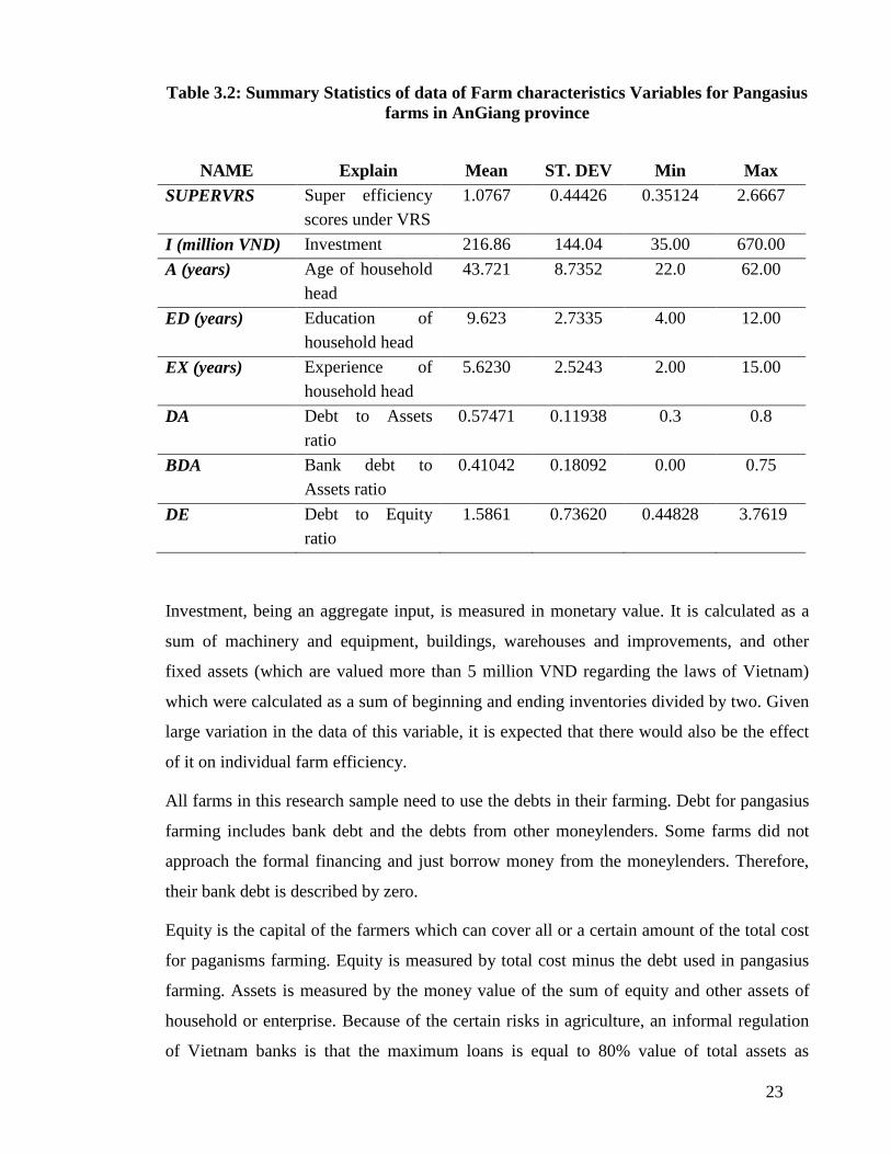
Table 3.2 provides summary-descriptive statistics for variables that were used in the

estimation of the relationship between the farm-specific variables that were hypothesized to

influence technical efficiency and the technical efficiency scores.

23

Table 3.2: Summary Statistics of data of Farm characteristics Variables for Pangasius

farms in AnGiang province

NAME Explain Mean ST. DEV Min Max

SUPERVRS Super efficiency

scores under VRS

1.0767 0.44426 0.35124 2.6667

I (million VND) Investment 216.86 144.04 35.00 670.00

A (years) Age of household

head

43.721 8.7352 22.0 62.00

ED (years) Education of

household head

9.623 2.7335 4.00 12.00

EX (years) Experience of

household head

5.6230 2.5243 2.00 15.00

DA Debt to Assets

ratio

0.57471 0.11938 0.3 0.8

BDA Bank debt to

Assets ratio

0.41042 0.18092 0.00 0.75

DE Debt to Equity

ratio

1.5861 0.73620 0.44828 3.7619

Investment, being an aggregate input, is measured in monetary value. It is calculated as a

sum of machinery and equipment, buildings, warehouses and improvements, and other

fixed assets (which are valued more than 5 million VND regarding the laws of Vietnam)

which were calculated as a sum of beginning and ending inventories divided by two. Given

large variation in the data of this variable, it is expected that there would also be the effect

of it on individual farm efficiency.

All farms in this research sample need to use the debts in their farming. Debt for pangasius

farming includes bank debt and the debts from other moneylenders. Some farms did not

approach the formal financing and just borrow money from the moneylenders. Therefore,

their bank debt is described by zero.

Equity is the capital of the farmers which can cover all or a certain amount of the total cost

for paganisms farming. Equity is measured by total cost minus the debt used in pangasius

farming. Assets is measured by the money value of the sum of equity and other assets of

household or enterprise. Because of the certain risks in agriculture, an informal regulation

of Vietnam banks is that the maximum loans is equal to 80% value of total assets as

24

collateral for the banks. Therefore, the DA ratio and BDA ratio have more small variations

in comparison to DE ratio in this research since they are all less than 1. DE ratio is expected

to have the effect on individual farm efficiency since it has larger variation in the data of

this variable.

25

CHAPTER 4: RESULTS

This chapter consists of two sections. First, the distribution of farm technical and scale

efficiency scores and characteristics of efficiency scores by each region and by pond size

are presented. Then, the relationship between farm super efficiency scores under the

assumption of variable returns-to-scale and farm-specific factors including farm financial

variables are estimated using the OLS model in Shazam. In addition, this chapter present

the results from testing of heteroscedasticity of the errors, test for omitted regressors and/or

wrong functional form and hypothesis testing,

4.1. Efficiency Scores

Farm technical efficiency (TE) scores under the assumptions of CRS and VRS and scale

efficiency (SE) scores were estimated using super DEA input oriented model. The

distributions of the scores are presented in Tables 4.1. Mean, standard deviation, minimum,

and maximum levels of TE and SE scores by regions are reported in Tables 4.2, 4.3, and

4.4 and by pond sizes are presented in Tables 4.5, 4.6 and 4.7.

From Table 4.1, Mean total technical efficiency for all farms is 0.595. It can be said that,

on average, pangasius farmers in An Giang province are producing pangasius at about

59.5% of the potential frontier production levels at the present state of technology and input

levels. It also means that farms can reduce their inputs by 40.5% and still produce the same

level of output. The number of super technically efficient farms (i.e., farms operating on the

production frontier) under the assumption of CRS was 8 (13.12%). Approximately 32.8%

of the farms exhibited TE scores less than 0.40, and 24.6% of the farms exhibited TE scores

from larger than 0.60 to less than 1.

Individual Super TE scores under the assumption of VRS ranged from 0.345 to 2.667

which show considerable variability among farms. Mean total super TE score for all farms

is 1.0576 and standard deviation of 0.443 indicates that farms can increase input usage by

5.76% and still be within the technology defined by the other farms in the sample. As can

be seen in table 4.1, TE scores under the assumption of variable returns-to-scale (TESVRS)

are considerably higher than TESCRS scores. These results suggest that the significant

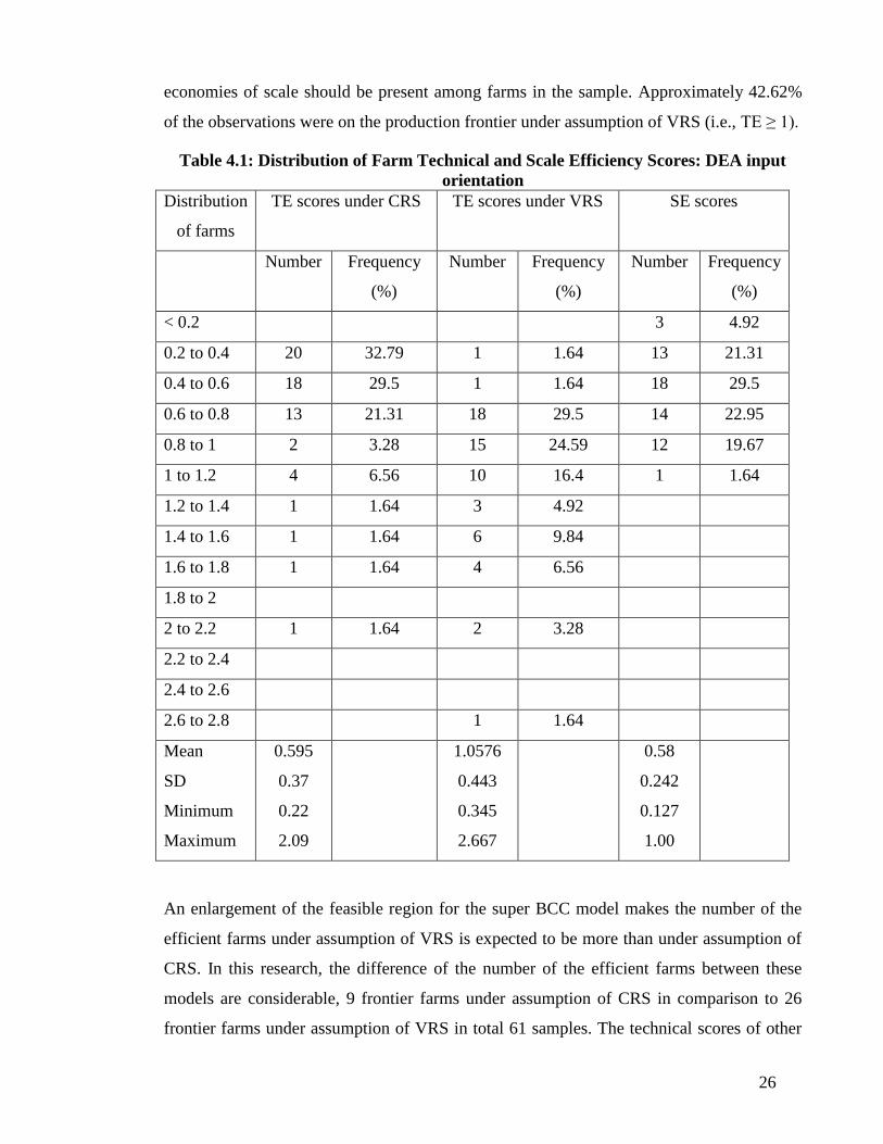
26

economies of scale should be present among farms in the sample. Approximately 42.62%

of the observations were on the production frontier under assumption of VRS (i.e., TE ≥ 1).

Table 4.1: Distribution of Farm Technical and Scale Efficiency Scores: DEA input

orientation

Distribution

of farms

TE scores under CRS TE scores under VRS SE scores

Number Frequency

(%)

Number Frequency

(%)

Number Frequency

(%)

< 0.2 3 4.92

0.2 to 0.4 20 32.79 1 1.64 13 21.31

0.4 to 0.6 18 29.5 1 1.64 18 29.5

0.6 to 0.8 13 21.31 18 29.5 14 22.95

0.8 to 1 2 3.28 15 24.59 12 19.67

1 to 1.2 4 6.56 10 16.4 1 1.64

1.2 to 1.4 1 1.64 3 4.92

1.4 to 1.6 1 1.64 6 9.84

1.6 to 1.8 1 1.64 4 6.56

1.8 to 2

2 to 2.2 1 1.64 2 3.28

2.2 to 2.4

2.4 to 2.6

2.6 to 2.8 1 1.64

Mean

SD

Minimum

Maximum

0.595

0.37

0.22

2.09

1.0576

0.443

0.345

2.667

0.58

0.242

0.127

1.00

An enlargement of the feasible region for the super BCC model makes the number of the

efficient farms under assumption of VRS is expected to be more than under assumption of

CRS. In this research, the difference of the number of the efficient farms between these

models are considerable, 9 frontier farms under assumption of CRS in comparison to 26

frontier farms under assumption of VRS in total 61 samples. The technical scores of other

27

farms in the sample under VRS also were improved in comparison to those under CRS.

There was only 1 farm (1.64%) exhibited TE scores less than 0.4 and 1 farm has score from

0.4 to less than 0.6, which mean 59 on 61 farms exhibited scores from 0.6 to less than 1.

4.1.1. Technical eficiency scores by region

Analyzing TE scores under CRS and VRS by regions are presented in Table 4.2, 4.3 and

4.4. It can be seen that under both CRS and VRS assumption, Region 2 had the highest

mean levels of TE scores, while the lowest cores belong to Region 1. Mean technical

efficiency scores under the assumption of variable returns-to-scale (TESVRS) with the

range goes from 0.945 for Region 1 to 1.036 for Region 3 and 1.2 in Region 2. The number

of frontier farms in Region 2 under VRS and CRS are also highest, 11 and 4 farms,

respectively, in comparison to those of Region 1, 7 and 1 farms, and Region 3, 7 and 3

farms, respectively. These results indicate that Region 2 and 3 exist the potential gains from

improving technical efficiency for farms in the sample, especially for the farms in Region

2, Chau Phu district.

Scale efficiency multiplied by the technical efficiency measured under VRS equals

technical efficiency under assumption of CRS Scale efficiency (SE). A farm can thus be

scale efficient (SE = 1) but not lie on the TEVRS or TECRS efficiency frontiers. There

were differences between TEVRS ands SE in the sample. The correlation coefficient

between technical and scale efficiency is – 0.178, indicating only a moderately negative

relationship between the two measures. The decomposition of the technical efficiency

measure show that pure technical inefficiency was the primary cause of technical

inefficiency. Scale efficiency scores varied from 0.127 to 1.00 with an average measure of

0.58 and standard deviation of 0.242. The scale efficiency level of 0.58 indicates that the

average farm is 42% scale inefficient of Pangasius farming in the sample. Individual

analysis of the farms indicate that 6.56% of the total sample farms had decreasing returns to

scale (DRS), indicating that the output levels of these farms would expand by a smaller

percentage then their inputs. One important finding is 91.8% of the sample pangasius farms

exhibits increasing returns to scale (IRS). This indicates that when these farms expand

their input levels by a certain percentage, their output level would expand by a larger

percentage. This result also indicate that these IRS farms operated at below optimal scale.

The percentage of scale efficient farms were very low : only 1 farm of the farms were fully

scale efficient, and 9.84% of the farms had SE scores higher than 0.95. Over all,

28

approximately 78.7% of the observations exhibited scale measures less than 0.80, and about

9.84% of the farms had SE scores 0.8 and 0.95. These above results mean the largest

increase in technical efficiency in the sample farms could be obtained by eliminating the

problem of increasing return to scales.

Table 4.2: Technical efficiency and Scale efficiency scores of Region 1

DMU

Region 1 – An Phu district

TECRS

scores

TE VRS

Scores and

Ranking

Scale

efficiency

Scores

TE NIRS

Scores

TE NDRS

Scores

Scale

Efficiency

A01 0.46 0.99 (22) 0.47 0.46 0.99 IRS

A02 0.25 0.82 (31) 0.30 0.25 0.82 IRS

A03 0.70 2.14 (2) 0.33 0.70 2.14 IRS

A04 1.14 1.41 (11) 0.81 1.14 1.41 IRS

A05 0.36 1.48 (10) 0.25 0.36 1.48 IRS

A06 0.36 1.13 (18) 0.32 0.36 1.13 IRS

A07 0.41 0.70 (39) 0.59 0.41 0.70 IRS

A08 0.47 0.63 (42) 0.74 0.47 0.63 IRS

A09 0.61 0.61 (44) 1.00 0.61 0.61 CRS

A10 0.56 1.16 (17) 0.48 0.56 1.16 IRS

A11 0.81 0.97 (23) 0.83 0.81 0.97 IRS

A12 0.52 1.41 (11) 0.37 0.52 1.41 IRS

A13 0.24 0.71 (38) 0.34 0.24 0.71 IRS

A14 0.51 1.03 (20) 0.50 0.51 1.03 IRS

A15 0.42 0.64 (41) 0.65 0.42 0.64 IRS

A16 0.22 0.61 (44) 0.36 0.22 0.61 IRS

A17 0.63 0.68 (40) 0.93 0.63 0.68 IRS

A18 0.29 0.62 (43) 0.47 0.29 0.62 IRS

A19 0.39 0.53 (45) 0.74 0.39 0.53 IRS

A20 0.47 0.79 (32) 0.59 0.47 0.79 IRS

A21 0.48 0.78 (33) 0.61 0.48 0.78 IRS

Mean 0.49 0.945 0.555 0.49 0.953

SD 0.212 0.4 0.22 0.218 0.408

Min 0.22 0.53 0.245 0.22 0.533

Max 1.143 2.14 1.00 1.143 2.145

29

Table 4.3: Technical efficiency and Scale efficiency scores of Region 2

DMU

Region 2 - Chau Phu district

TE CRS

scores

TE VRS

Scores and

Ranking

Scale

efficiency

Scores

TE NIRS

Scores

TE NDRS

Scores

Scale

Efficiency

C01 1.09 1.57 (8) 0.69 1.09 1.57 IRS

C02 0.48 1.30 (13) 0.37 0.48 1.30 IRS

C03 0.50 1.19 (15) 0.42 0.50 1.19 IRS

C04 0.68 1.17 (16) 0.58 0.68 1.17 IRS

C05 0.69 0.92 (25) 0.75 0.69 0.92 IRS

C06 0.46 1.19 (15) 0.39 0.46 1.19 IRS

C07 0.43 0.85 (28) 0.50 0.43 0.85 IRS

C08 0.73 0.75 (35) 0.98 0.73 0.75 IRS

C09 0.42 0.74 (36) 0.57 0.42 0.74 IRS

C10 0.37 0.88 (27) 0.42 0.37 0.88 IRS

C11 0.78 1.00 (21) 0.78 0.78 1.00 IRS

C12 0.27 2.09 (3) 0.13 0.27 2.09 IRS

C13 1.26 1.79 (4) 0.70 1.79 1.26 DRS

C14 1.71 1.79 (4) 0.96 1.71 1.79 IRS

C15 0.35 0.84 (29) 0.42 0.35 0.84 IRS

C16 1.15 1.39 (12) 0.83 1.15 1.39 IRS

C17 0.30 1.13 (18) 0.27 0.30 1.13 IRS

C18 0.41 0.84 (29) 0.48 0.41 0.84 IRS

C19 0.61 0.94 (24) 0.65 0.61 0.94 IRS

C20 0.31 1.61 (6) 0.19 0.31 1.61 IRS

Mean 0.65 1.2 0.554 0.676 1.17

SD 0.38 0.39 0.238 0.44 0.367

Min 0.266 0.73 0.127 0.266 0.737

Max 1.707 2.086 0.975 1.79 2.09

30

Table 4.4: Technical efficiency and Scale efficiency scores of Region 3

DMU

Region 3 – Long Xuyen city

TE CRS

scores

TE VRS

Scores and

Ranking

Scale

efficiency

Scores

TE NIRS

Scores

TE NDRS

Scores

Scale

Efficiency

L01 0.32 0.90 (26) 0.35 0.32 0.90 IRS

L02 0.25 1.00 (21) 0.25 0.25 1.00 IRS

L03 0.30 1.76 (5) 0.17 0.30 1.76 IRS

L04 0.86 0.94 (24) 0.92 0.86 0.94 IRS

L05 0.31 0.76 (34) 0.41 0.31 0.76 IRS

L06 0.63 1.58 (7) 0.40 0.63 1.58 IRS

L07 0.76 1.06 (19) 0.72 0.76 1.06 IRS

L08 0.31 0.94 (24) 0.33 0.31 0.94 IRS

L09 0.70 0.94 (24) 0.75 0.70 0.94 IRS

L10 0.29 0.35 (46) 0.85 0.29 0.35 IRS

L11 0.75 0.76 (34) 0.99 0.75 0.76 IRS

L12 0.29 0.68 (40) 0.43 0.29 0.68 IRS

L13 1.47 1.49 (9) 0.99 1.49 1.47 DRS

L14 2.09 2.67 (1) 0.78 2.67 2.09 DRS

L15 0.40 0.85 (28) 0.47 0.40 0.85 IRS

L16 0.29 0.64 (41) 0.44 0.29 0.64 IRS

L17 0.79 0.83 (30) 0.95 0.79 0.83 IRS

L18 0.46 0.63 (42) 0.73 0.46 0.63 IRS

L19 1.16 1.21 (14) 0.96 1.21 1.16 DRS

L20 0.56 0.73 (37) 0.76 0.56 0.73 IRS

Mean 0.65 1.036 0.632 0.682 1.003

SD 0.471 0.513 0.27 0.575 0.423

Min 0.25 0.345 0.17 0.25 0.345

Max 2.09 2.667 0.991 2.667 2.09

Analysis of SE scores by regions indicates that mean SE scores varied from 0.55 to 0.632,

with average standard deviation varying from 0.22 in Region 1 to 0.27 in Region 2. Among

the regions, Region 3 had the highest mean score with 4 farms had SE scores higher than

0.95 while Region 1 had only 1 farm which is scale efficient. These results indicate that

most farms in each region operate at an inefficient scale and, therefore, significant

31

improvements in scale efficiency can be accomplished by most farms in the sample by

changing the scale of their operation.

In order to examine differences in the estimated efficiency between the regions, “ANOVA

Test” for homogeneity of mean scores of TECRS, TEVRS, and SE scores between the

regions were performed in Excel.

The results of the F-tests show that the equality of means for all three regions for TECRS,

TEVRS, and SE could not be rejected at the 5% significance level. These results indicate

that average TECRS, TEVRS and SE scores are statistically similar among all of the

regions.

Table 4.5 reported the results of the tests of comparison the mean of technical efficiency

scores between regions. The same letter by the regions indicates that the mean efficiency

scores of those regions are not significantly different.

Table 4.5: Mean of technical efficiency scores between regions

Region TECRS TEVRS SE

An Phu (1) 0.49 A 0.9447 A 0.5562 A

Chau Phu (2) 0.65 A 1.199 B 0.554 A

Long Xuyen (3) 0.6495 A 1.036 B 0.6325 A

The results for each region indicate that under the assumption of VRS, Region 1 has lower

average TE scores than Region 2 and Region 3. There is no evidence to reject the

hypothesis at the 5% significance level of difference in mean TE scores under CRS and SE

scores between all three regions.

4.1.2. Efficiency – Pond size relationship

In order to examine how efficiency scores vary with pond size, Pangasius ponds were

classified into 3 size groups as can be seen in Table 4.6, 4.7 and 4.8.

As can be seen in tables 4.6 to 4.8, under consumption of CRS, the most efficient farms

were the largest farms, while under VRS, the most efficient farms were the smallest ones.

Turning to the scale efficiency, the smallest farms were in average the least efficient and

the largest farms were the most efficient.

32

ANOVA analysis for each farm size group was conducted and showed that pond size had a

statistically significant impact on efficiency. The results of the F-tests show that the

equality of means for all three pond sizes for TESCRS is rejected at the 1% significance

level. For TESVRS, the equality of the means is rejected at the 5% significance level.

Equality of the means is also rejected for SE. This result indicates that average SE scores

are statistically different among all of the pond sizes.

Table 4.6: Efficiency scores of Pangasius farmers according to Pond size less than 4000m2

DMU Area

(m2)

TECRS

scores

TEVRS

Scores

Scale

efficiency

Scores

TE NIRS

Scores

TE NDRS

Scores

Scale

Efficiency

A01 1000 0.46 0.99 0.47 0.46 0.99 IRS

A06 1000 0.36 1.13 0.32 0.36 1.13 IRS

L03 1000 0.3 1.76 0.17 0.3 1.76 IRS

C02 1200 0.48 1.3 0.37 0.48 1.3 IRS

C12 1800 0.27 2.09 0.13 0.27 2.09 IRS

A02 2000 0.25 0.82 0.3 0.25 0.82 IRS

A03 2000 0.7 2.14 0.33 0.7 2.14 IRS

A10 2000 0.56 1.16 0.48 0.56 1.16 IRS

A16 2000 0.22 0.61 0.36 0.22 0.61 IRS

C06 2000 0.46 1.19 0.39 0.46 1.19 IRS

C20 2000 0.31 1.61 0.19 0.31 1.61 IRS

A13 2200 0.24 0.71 0.34 0.24 0.71 IRS

A05 2500 0.36 1.48 0.25 0.36 1.48 IRS

A18 2500 0.29 0.62 0.47 0.29 0.62 IRS

A20 2500 0.47 0.79 0.59 0.47 0.79 IRS

C03 2500 0.5 1.19 0.42 0.5 1.19 IRS

L06 2500 0.63 1.58 0.4 0.63 1.58 IRS

C18 3000 0.41 0.84 0.48 0.41 0.84 IRS

L02 3000 0.25 1 0.25 0.25 1 IRS

A12 3500 0.52 1.41 0.37 0.52 1.41 IRS

A21 3500 0.48 0.78 0.61 0.48 0.78 IRS

C01 3500 1.09 1.57 0.69 1.09 1.57 IRS

Mean 2236.3 0.4368 1.2168 0.3809 0.4368 1.2168

SD 771.24 0.1973 0.4471 0.1418 0.1973 0.61

Min 1000 0.22 0.61 0.13 0.22 2.14

Max 3500 1.09 2.14 0.69 1.09

33

Table 4.7: Efficiency scores of Pangasius farmers according to Pond size less than 7000m2

DMU Area

(m2)

TECRS

scores

TEVRS

Scores

Scale

efficiency

Scores

TE NIRS

Scores

TE NDRS

Scores

Scale

Efficiency

A07 4000 0.41 0.7 0.59 0.41 0.7 IRS

A15 4000 0.42 0.64 0.65 0.42 0.64 IRS

C04 4000 0.68 1.17 0.58 0.68 1.17 IRS

C15 4000 0.35 0.84 0.42 0.35 0.84 IRS

C17 4000 0.3 1.13 0.27 0.3 1.13 IRS

L05 4000 0.31 0.76 0.41 0.31 0.76 IRS

L08 4000 0.31 0.94 0.33 0.31 0.94 IRS

L18 4000 0.46 0.63 0.73 0.46 0.63 IRS

A14 4800 0.51 1.03 0.5 0.51 1.03 IRS

C05 5000 0.69 0.92 0.75 0.69 0.92 IRS

C07 5000 0.43 0.85 0.5 0.43 0.85 IRS

C10 5000 0.37 0.88 0.42 0.37 0.88 IRS

C16 5000 1.15 1.39 0.83 1.15 1.39 IRS

A08 5500 0.47 0.63 0.74 0.47 0.63 IRS

L16 5500 0.29 0.64 0.44 0.29 0.64 IRS

L01 6000 0.32 0.9 0.35 0.32 0.9 IRS

L09 6000 0.7 0.94 0.75 0.7 0.94 IRS

L12 6000 0.29 0.68 0.43 0.29 0.68 IRS

L20 6000 0.56 0.73 0.76 0.56 0.73 IRS

A11 6080 0.81 0.97 0.83 0.81 0.97 IRS

Mean 4894 0.4915 0.8685 0.564 0.4915 0.8685

SD 842.35 0.2204 0.2046 0.1791 0.2204 0.2046

Min 4000 0.29 0.63 0.27 0.29 0.63

Max 6080 1.15 1.39 0.83 1.15 1.39

34

Table 4.8: Efficiency scores of Pangasius farmers according to Pond size larger than 7000m2

DMU Area

(m2)

TECRS

scores

TEVRS

Scores

Scale

efficiency

Scores

TE NIRS

Scores

TE NDRS

Scores

Scale

Efficiency

A09 7000 0.61 0.61 1 0.61 0.61 CRS

A19 7000 0.39 0.53 0.74 0.39 0.53 IRS

C19 7000 0.61 0.94 0.65 0.61 0.94 IRS

L07 7000 0.76 1.06 0.72 0.76 1.06 IRS

L15 7000 0.4 0.85 0.47 0.4 0.85 IRS

A04 9000 1.14 1.41 0.81 1.14 1.41 IRS

A17 9000 0.63 0.68 0.93 0.63 0.68 IRS

C09 10000 0.42 0.74 0.57 0.42 0.74 IRS

C11 10000 0.78 1 0.78 0.78 1 IRS

L10 15000 0.29 0.35 0.85 0.29 0.35 IRS

L14 15000 2.09 2.67 0.78 2.67 2.09 DRS

C08 16000 0.73 0.75 0.98 0.73 0.75 IRS

L13 18000 1.47 1.49 0.99 1.49 1.47 DRS

L17 18000 0.79 0.83 0.95 0.79 0.83 IRS

L04 20000 0.86 0.94 0.92 0.86 0.94 IRS

C13 30000 1.26 1.79 0.7 1.79 1.26 DRS

C14 30000 1.71 1.79 0.96 1.71 1.79 IRS

L11 30000 0.75 0.76 0.99 0.75 0.76 IRS

L19 30000 1.16 1.21 0.96 1.21 1.16 DRS

Mean 15526.3 0.8868 1.0736 0.8289 0.9489 1.0115

SD 8758.28 0.4773 0.5544 0.1566 0.6004 0.4371

Min 7000 0.29 0.35 0.47 0.29 0.35

Max 30000 2.09 2.67 1 2.67 2.09

Comparison of the mean scores of three pond sizes groups under assumption of CRS

suggests that farms of the smallest size group are 50.56% and farms of 4000 to under 7000

m2

are 45% less than farms above 7000 m2, which are in average the most efficient.

However, farms under 4000 m2 are the best farms under consumption of VRS. They are

28.7% more efficient than farms of 4000- under 7000 m2, and by 12.3% more efficient than

farms above 7000 m2. The highest scale efficiency score was achieved by farms of the

largest size group. Farms under 4000 m2 are 54.2% and farms of 4000- under 7000 m

2 are

32.5% less efficient than farms above 7000 m2.

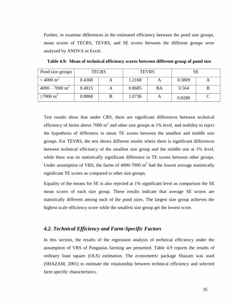
35

Further, to examine differences in the estimated efficiency between the pond size groups,

mean scores of TECRS, TEVRS, and SE scores between the different groups were

analyzed by ANOVA in Excel.

Table 4.9: Mean of technical efficiency scores between different group of pond size

Pond size groups TECRS TEVRS SE

< 4000 m2 0.4368 A 1.2168 A 0.3809 A

4000 – 7000 m2 0.4915 A 0.8685 BA 0.564 B

≥7000 m2 0.8868 B 1.0736 A 0.8289 C

Test results show that under CRS, there are significant differences between technical

efficiency of farms above 7000 m2 and other size groups at 1% level, and inability to reject

the hypothesis of difference in mean TE scores between the smallest and middle size

groups. For TEVRS, the test shows different results where there is significant differences

between technical efficiency of the smallest size group and the middle one at 1% level,

while there was no statistically significant difference in TE scores between other groups.

Under assumption of VRS, the farms of 4000-7000 m2 had the lowest average statistically

significant TE scores as compared to other size groups.

Equality of the means for SE is also rejected at 1% significant level as comparison the SE

mean scores of each size group. These results indicate that average SE scores are

statistically different among each of the pond sizes. The largest size group achieves the

highest scale efficiency score while the smallest size group get the lowest score.

4.2. Technical Efficiency and Farm-Specific Factors

In this section, the results of the regression analysis of technical efficiency under the

assumption of VRS of Pangasius farming are presented. Table 4.9 reports the results of

ordinary least square (OLS) estimation. The econometric package Shazam was used

(SHAZAM, 2001) to estimate the relationship between technical efficiency and selected

farm specific characteristics.

36

The translog production function is tested for significance. First, the null hypothesis that the

interactive terms have significant effects is tested. The F-test statistic, 0.55 with 21 and 25

degrees of freedom, suggests that the interactive terms should be removed from the model.

Then, the F-test is also used to test whether the second order terms have significant effects.

The test statistic, 1.07 with 7 and 46 degrees of freedom, are in favor of the absence of the

second order terms in the model.

4.2.1. Test for the heteroscedasticity of the errors by the Goldfeld-Quandt test:

Regression disturbances whose variances are not constant across observation are

heteroscedastic. Hereroscedasticity arises in numerous applications, in both cross-section

and times-series data. Hereroscedasticity poses potentially severe problems for inferences

based on least squares. It is useful to be able to test for homoscedasticity and if necessary,

modify our estimation procedures accordingly.

Several types of tests have been suggested. The Goldfeld-Quandt test is used to detect the

presence of hereroscedasticity in this research.

For the Goldfeld-Quandt test, we assume that the observations can be divided into two

groups that under the hypothesis of homoscedasticity, the disturbance variances would be

the same in the two groups, whereas under the alternative, the disturbance variances would

differ systematically.

The test is applied by dividing the sample into two subsets with n1 and n2 observations.

Denote the variance in the first subset by σ12 and the variance in the second subset by σ2

2.

The null hypothesis is H0: σ12

= σ22

and the alternative hypothesis is H1: σ12 > σ2

2.

To obtain statistically independent variance estimators, the regression is then estimated

separately with the two sets of observations. The test statistics is calculated as:

RSSE1 / (n 1 – K)

F [n1 – K, n 2 – K] =

RSSE2 / (n 2 – K)

Where RSSE1 and RSSE2 are the sum of squared errors from the first N1 and the last N2

observations respectively. Under the null hypothesis of homoscedasticity, this statistic has

an F distribution with n1 – K and n 2 – K degrees of freedom.

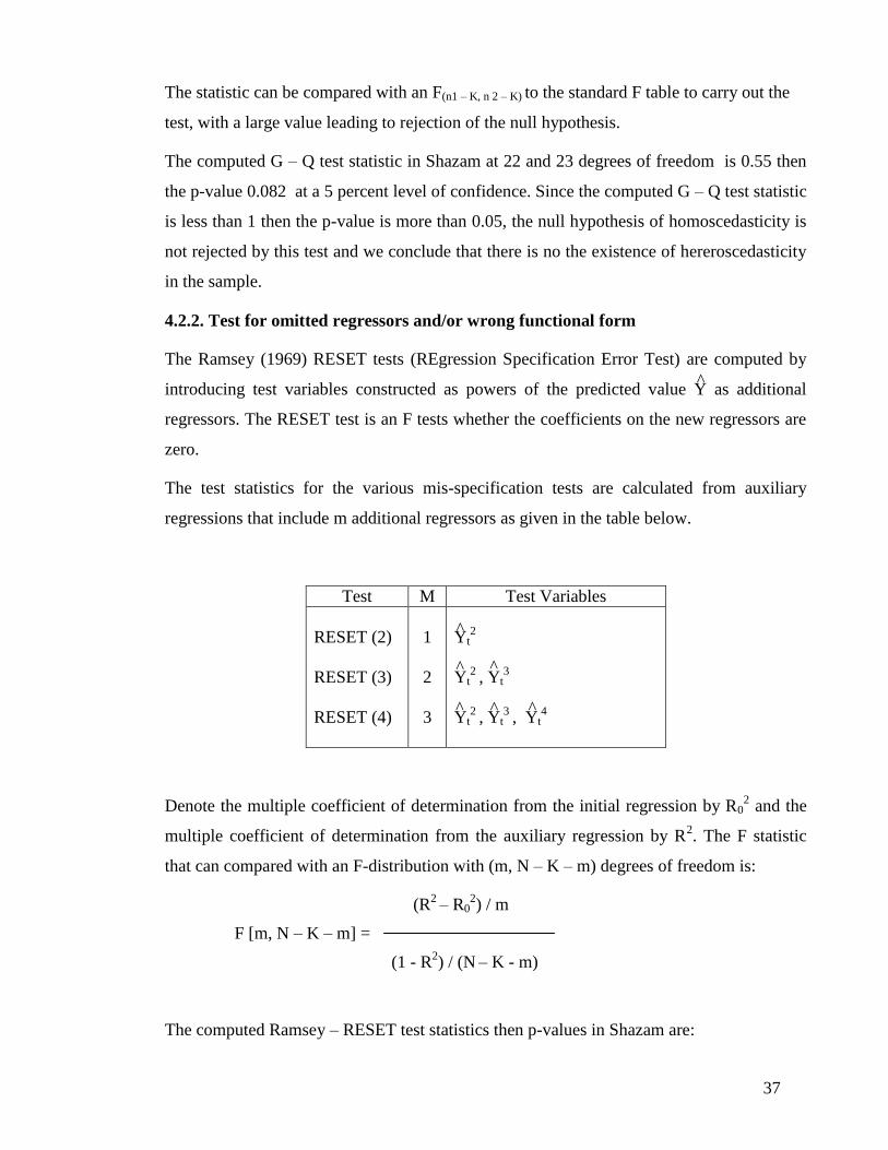
37

The statistic can be compared with an F(n1 – K, n 2 – K) to the standard F table to carry out the

test, with a large value leading to rejection of the null hypothesis.

The computed G – Q test statistic in Shazam at 22 and 23 degrees of freedom is 0.55 then

the p-value 0.082 at a 5 percent level of confidence. Since the computed G – Q test statistic

is less than 1 then the p-value is more than 0.05, the null hypothesis of homoscedasticity is

not rejected by this test and we conclude that there is no the existence of hereroscedasticity

in the sample.

4.2.2. Test for omitted regressors and/or wrong functional form

The Ramsey (1969) RESET tests (REgression Specification Error Test) are computed by

introducing test variables constructed as powers of the predicted value Y as additional

regressors. The RESET test is an F tests whether the coefficients on the new regressors are

zero.

The test statistics for the various mis-specification tests are calculated from auxiliary

regressions that include m additional regressors as given in the table below.

Test M Test Variables

RESET (2)

RESET (3)

RESET (4)

1

2

3

Yt2

Yt2

, Yt3

Yt2

, Yt3

, Yt4

Denote the multiple coefficient of determination from the initial regression by R02 and the

multiple coefficient of determination from the auxiliary regression by R2. The F statistic

that can compared with an F-distribution with (m, N – K – m) degrees of freedom is:

(R2

– R02) / m

F [m, N – K – m] =

(1 - R2) / (N – K - m)

The computed Ramsey – RESET test statistics then p-values in Shazam are:

^

^

^

^

^

^ ^

38

RESET(2)= 2.4253 - F WITH DF1= 1 AND DF2= 52 P-VALUE= 0.125

RESET(3)= 1.9689 - F WITH DF1= 2 AND DF2= 51 P-VALUE= 0.150

RESET(4)= 1.3108 - F WITH DF1= 3 AND DF2= 50 P-VALUE= 0.281

Since the computed p-values are more than 0.05, the null hypothesis of the coefficients on

the new regressors are zero is not rejected by this test and we conclude that the estimated

model is well specified.

4.2.3. Ordinary least squares estimation:

Ordinary least squares (OLS) estimates of the parameters of the model are presented in

Table 4.9. With the R2 value of 0.54, the independent variables used in the model were able

to explain 54% of the variation in the technical efficiency scores under VRS for the study

area.

Table 4.10: Parameter estimate and test statistics of Ordinary least squares model

Variables Parameters Estimated coefficients t-value

Constant α0 - 0.59064 - 0.7926

Investment αI 0.13953 2.083**

Age of household head αA - 0.15084 - 0.8799

Education of household head αED 0.080951 0.6801

Experience in Pangasius farming αEX 0.19583 2.241**

Debt to assets ratio αDA 0.34494 1.895***

Bank debt to asset ratio αBDA 0.000002 1.496

Debt to equity ratio αDE 0.36064 3.550*

* Statistically significant at the level of 1%

** Statistically significant at the level of 5%

*** Statistically significant at the level of 10%

t- statistics are calculated, with the null hypothesis that a parameter is zero, which means

that the estimated variable has no effect on the dependent variable given that the other

variables are in the model.

39

Result indicates that the effect of investment for Pangasius farming is significant at the 5%

level. Increased investment for applying modern machines to mix the feed for fish and

equipment in operating such as the pumps to change water in fish ponds in the last month

of cultivating, warehouses and improvement of ponds before starting the new crop, lead to

better performance of technical efficiency.

Variables Age, Education, which measured by schooling years, and Experience, which

measured in number of years of the head of the household were included in the model to

estimate the effects of socio-economic factors on the level of technical efficiency. It is

believed that increased age and farming experience go together with higher level of

educational achievement may lead to a better assessment in using inputs efficiently and

making complex and important decisions in farm investment or farm operating. Results in

Table 4.9, however, show that only variable of Experience has an expected sign and

statistically significant at the level 5% confidence. This result indicates that farming

experience has an effect on a farmers‟ ability to allocate resources or decision to invest

their farms more efficiently. Variable Education level has an expected sign, but it is not

statistically significant. Variable Age of the head of household has a negative influence on

technical efficiency, but it is also not significant in statistic. These contradictory results

might be explain due to the fact that although older farmers might have more experience

than younger farmers, they may be more careful and conservative in adopting new

technology, therefore, lead to less efficiency.

Leverage variables DA (current debt-to-asset ratios in this research) was statistically

significant at the 10% level, while no significant influence of variable BDA (current bank

debt-to asset ratio) is found in the sample. These results indicate that although total debt to

asset ratios has certain effects on technical efficiency, the level of bank debt in comparison

to the total debt has no effects on technical efficiency. As mentioned in chapter 3, informal

financing is still common in Vietnam, especially in agriculture sector. Besides, the

difficulties in approaching the credit from the bank and constraints of collateral assets are

also the important reasons to explain why farmers do not base their farming in only the

formal financing. However, of course, without or less collateral assets, farmers need to pay

more for the interest rate for the moneylenders.

Variable DA has a positive influence on technical efficiency. The result supports the free

cash flow concept and, contradicts the agency cost concept in finance. The farmers are

40

indebted face to the pressure of their repayment obligations and therefore, they are

motivated to improve their efficiency. In practical, this result suggests that benefits of debt

motivate managers to become more efficient because farmers who are indebted can

generate enough financial resources to cover their operating expenses. It is appropriate in

the case of Pangasius farming which need the high cost for operating.

As expected, the debt to equity ratio (DE) variable has a positive impact on technical

efficiency and is significant at the 1% level. As mentioned before, variable DE has more

potential effect to the technical efficiency in comparison to variable DA. Equity is mainly

kept in cash which is using to buy and pay for inputs serves for farming, while Assets

include the fixed properties (i.e land, houses, equipment) that are not easy to transform to

cash in a short time. Therefore, it is easier to see the effects of DE on technical efficiency

than DA.

In short, the results indicate that financial exposure (as measured by DA and DE) is a

source of efficiency for all pangasius farms in the sample, the increase in indebtedness is

positively related to the technical efficiency scores for those farms.

41

CHAPTER 5: SUMMARY AND CONCLUSIONS

Thesis Summary

This research uses the DEA method to estimate the technical efficiency and scale efficiency

of selected Pangasius farms of the An Giang province, the leading region of Pangasius

farming in the Mekong Delta of Vietnam. Cross-sectional data of directly interviews from

61 farms from three geographic regions were used in the study. To estimate the technical

efficiency, the data for each farm in the sample were aggregated into six inputs (Labor,

Fuel and oil, Electricity, Chemicals, Seed and Feed) and one output (Pangasius production).

Farm individual technical efficiency scores were used in a regression model to reveal the

relationship between the technical efficiency under assumption of variable returns to scale

and different farm-specific characteristics that including farm‟s financial variables.

Variables hypothesized to influence technical efficiency included farm investment, age,

education, experience of household head, total debt-to-asset ratios, bank-debt-to-asset

ratios, total debt-to-equity ratios .

Results and discussions

Findings of the research showed that, on average, Pangasius farms under the analysis were

0.595 technically efficient under the assumption of constant returns-to-scale (CRS) with

TECRS ranged from a minimum of 0.22 to a maximum 2.9, 1.058 technically efficient

under the assumption of variable returns-to-scale (VRS) with TEVRS ranged between 0.34

and 2.67, and 0.58 scale efficient with SE ranged between 0.13 and 1.00. Minimum and

maximum values of efficiency score show considerable variability among farms. Mean

technical efficiency under CRS suggests that the inputs used by Pangasius farms can be

reduced by 40.5% and produce the same level of output if each farm in the sample was

producing on the the efficient frontier at constant returns to scale. When adjusted for farm

size, many farms have a higher level of VRS technical efficiency, 1.058 on average. These

mean levels of technical efficiency measures are higher in comparison to technical

efficiencies of the Catfish farms in Chicot, Arkansas, which were calculated as 0.57 and

0.73, respectively (Kaliba and Engle, 2006). However, techincal efficencis of Pangasius

farming are much lower in comparison to the technical efficiencies of aquaculture sector in

other countries, which was estimated for trout pond farming in the Black Sea Region,

42

Turkey which was estimated 0.82 (Cinemre (2006), for tilapia pond operations in

Philippines which was estimated as 0.83 (Kumar et al, 2004), for milkfish (Chanos chanos)

farming in pond in Taiwan (Chiang et al., 2004) which was estimated as 0.84 and for

Chinese fish farms polyculture and the prawn-carp farming of Bangladesh, which were

estimated 0.83 (Sharma, 1999) and 0.85 (Ferdous Alam, Murshed-e-Jahan, K. (2008),

respectively. This indicates that consierable scope to raise Pangasius production using the

existing lavel of input use and technology. The scale efficiency level of 0.58 indicates that

42% of all farms in the sample is scale inefficient. Mean level of scale efficiency of

Pangasius farming is also lower in comparison to that measure for the Catfish farms in

Chicot, Arkansas, which were calculated as 0.77 (Kaliba and Engle, 2006) and for the

prawn-carp farming of Bangladesh, which were estimated 0.88 (Ferdous Alam, Murshed-e-

Jahan, K. (2008). The low scale efficiency in comparison to the VRS technical efficiency

suggests that inefficiencies of Pangasius farms are mostly due to scale inefficiency rather

than inefficient management pratices. The observed technical inefficiency can be

eliminated and improved by eliminating the problem of increasing returns to scale as about

92% of the sample pangasius farms exhibits increasing returns to scale (IRS). Therefore,

the Pangasius efficiency could be increased by increasing the scale of the average farms in

the sample.

Tests for homogeneity of variance between efficiency ratios among the regions indicated

that the equality of means for technical efficiency under CRS and VRS and scale efficiency

scores for all three regions could not be rejected at the 5% significance level, which

indicates that average TECRS, TEVRS and SE scores are statistically similar among all of

the regions. The results for each region indicated that The results for each region indicate

that under the assumption of VRS, Region 1 has lower average TE scores than Region 2

and Region 3.

The results of the F-tests for whether the existence of the impact of pond size groups on the

efficiency show that the equality of means for all three pond sizes for TESCRS is rejected

at the 1% significance level and rejected at the 5% significance level for TESVRS. Under

CRS, the farms in the largest group (>7000 m2) are more technical efficiency than other

size groups. Under VRS, the farms of 4000-7000 m2 had the lowest average statistically

significant TE scores as compared to other size groups while there is no statistically

difference between the farms of the largest and smallest size groups. Equality of the means

43

is also rejected for SE indicating that average SE scores are statistically different among all

of the pond sizes. The largest size group (>7000 m2) achieves the highest scale efficiency

score while the smallest size group (< 4000 m2) get the lowest score.

Farm technical efficiency was found to be influenced by farm indebtedness. The resuls

indicate that financial exposure is a source of efficiency for all Pangasius farms in the

sample. In other words, the increase in debts positively influences the technical efficiency

of those farms. The significant positive relationships were found between technical

efficiency and the short-term debt-to-asset ratio, and between technical efficiency and the

short-term debt-to-equity ratio while the variable bank debt-to-asset ratio was not

statistically significant. This can be explained as the farmers have the constraints in

accessing the bank credit and try to borrow money from the other informal financing. The

results for the short-term debt-to-asset ratio and the short-term debt-to-equity ratio are

consistent with the free cash flow and do not support the agency cost concepts of finance

theory.

Technical efficiency is positively influenced by farm investment. Increased cost for

applying modern machines and equipment in operating as well as improvement of ponds

before starting the new crop, lead to better performance of technical efficiency.

The experience of household head measured by the years of pangasius farming has positive

effects on technical efficiency indicates that the more experiences the farmers have had in

previous time of farming, the more efficiency those farms will have.

Conclusion remarks:

The main findings of this research are: (1) technical efficiencies of Pangasius farming in

Vietnam was estimated under assumption of constant returns to scale and variable returns

to scale as 0.595 and 1.058, respectively; (2) estimated scale efficiency is 0.58 which

exhitbits increasing returns to scale; (3) financial variables (indebtedness of farms) are

among the farm specific factors influenced on technical efficiency and the sign of effects of

these financial variables is positive.

Pangasius farming is continuing to be one of the important sectors of the aquaculture

industry in Vietnam. Due to the very favourable conditions in the South of Vietnam,

especially in the Mekong Delta, i.e., warm weather and water all seasons in the year,

44

Pangasius grows well in this region. Moreover, with its characteristics of adapting well

with the environment and high ability to resist most of the diseases, Pangasius is farmed

commonly in the Mekong Delta since 1990 and intensively since the reform of Vietnam to

enlarge the international trade. However, the Pangasius industry is still young. The results

of this research suggest that technical efficiency of Pangasius farms in Vietnam is still not

on a par with similar aquacultural operations in other countries and in Asia. More efficient

use of inputs, such as feed, seed, and labor as well as increasing the scale of farms may in

the future be the key for lifting productivity and hence profitability of Pangasius farming in

Vietnam. Moreover, this research suggests the positive role of debt in Pangasius farming in

the Mekong Delta of Vietnam. These findings might be informative for policy formation

and future researchs.

45

REFERENCES

Aigner, D.J., Lovell, C.A.K., Schmidt, P.J. (1977). Formulation and Estimation of

Stochastic Frontier Production Function Models. Journal of Econometrics, 6: 21–37.

Andersen, P. and Petersen. N.C. (1993) A Procedure for Ranking Efficient Units in Data

Envelopment Analysis. Management Science 39 (10): 1261-1264.

Andreu, M.L., Featherstone, A.M., Langemeier M.R. (2006). Impacts of Financial variables

on Production in Kansas Farms Efficiciencies. Selected Paper Prepared for

Presentation at the American Agricultural Economics Association Annual Meeting,

Long Beach, California, July 23-26.

Banker, R.D., A. Charnes, and W.W. Cooper. 1984. "Some Models for Estimating

Technical and Scale Inefficiencies in Data Envelopment Analysis." Management

Science 30(9): 1078-1092.

Banker, R.D. and R.M. Thrall. 1992. "Estimation of Returns to Scale Using Data

Envelopment Analysis." European Journal of Operational Research 62(1): 35-44.

Banker, R.D. and Morey, R. (1986). The Use of Categorical Variables in Data

Envelopment Analysis. Management Science, 32(12): 1613–1627.

Banker, R.D., I. Bardhan and Cooper, W.W. (1996). A note on returns to scale in DEA.

European Journal of Operational Research 88: 583-585.

Banker, R.D., Chang, H. (2006). The super-efficiency procedure for outlier identification,

not for ranking efficient units. European Journal of Operational Research,175: 1311-

1320.

Battese, G.E., Corra, G. (1977) Estimation of a Production Frontier Model with Application

to the Pastoral Zone of Easter Australia. Australian Journal of Agricultural

Economics, 21(3): 167–179.

Barry, P.J., C.B. Baker, and L.R. Sanint. 1981. "Farmers' Credit Risks and Liquidity

Management." American Journal of Agricultural Economics 63: 216-227.

Berzlepkina, I., Lansink, A.O., Huirne, R. (2004). Effects of debt on Moscow-region dairy

farm performance, 1996-2000. Paper presented at the minisimposium “Africultureal

transformation: Lessons from five trnsition countries” organised by Mansholt

Graduate School, October 28.

Charnes, A., W.W. Cooper, and E. Rhodes. 1978. Measuring the Efficiency of Decision

Making Units. European Journal of Operational Research 2(6): 429-444.

46

Charnes, A., Cooper, W.W. and Rhodes, E. (1981). Evaluating Program and Managerial

Efficiency: An Application of Data Envelopment Analysis to Program Follow

Through. Management Science, 27(6): 668–697.

Charnes, A., Clark, C.T., Cooper, W.W. and Golany, B. (1985). A Developmental Study of

Data Envelopment Analysis in Measuring the Efficiency of Maintenance Units in the

U.S. Air Forces in R.G. Thompson and R, N, Thrall, eds., Annals of Operations

Research, 2: 95–112.

Charnes, A., Cooper, W.W., Sun, D.B. and Huang, Z.M. (1990). Polyhectal Cone-ratio

models with an illustrative application to large commercial banks. Journal of

Econometrics, 46: 73–91.

Charnes, A., Cooper, W.W., Wei, Q.L. and Huang, Z.M. (1989). Cone Ratio Data

Envelopment Analysis and Multi-Objective Programming. International Journal of

Systems Science, 20(7): 1099–1118.

Chavas, J.P. and M. Aliber (1993). An Analysis of Economic Efficiency in Agriculture: A

Nonparametric Approach. Journal of Agricultural and Resource Economics 18(1): 1-

16.

Chen. Y. (2003). Ranking efficient units in DEA. The International Journal of

Management Science, 32: 213-219

Chen, Y. „Measuring super-efficiency in DEA in the presence of infeasibility‟, European

Journal of Operational Research, Vol. 161, (2005) pp. 545–551.

Cinemre, H.A., Ceyhan, V., K.,Demiryu¨rek, M., Bozog˘lu, Kilic, O. (2006). The cost

efficiency of trout farms in the Black Sea Region, Turkey. Aquaculture 251, 324-332.

Coelli, T., Rao, D.S.P., O‟Donnell, C.J., Battese, G.E., 2005. An Introduction to Efficiency

and Productivity Analysis (Second Edition). Springer Publishers, New York, USA.

(308 pp.).

Cooper, W.W., Seiford, L.M., Zhu, J. (2004) Data Envelopment Analysis History, Models

and Interpretations, in Hand book of Data Envelopment Analysis ed. Cooper W.W:,

Seiford L.M., Zhu J., Boston: Kluwer Academic Publishers.

Dey, M.M., Paraguas, P.J., Bimbao, G.B., Regaspi, P.B., 2000. Technical efficiency of

tilapia grow out pond operations in the Philippines. Aquaculture Economics and

Management 4, 33– 47.

Ellinger, P.N. and Barry P.J. 1991. "Agricultural Credit Delivery Costs at

Commercial Banks." Agricultural Finance Review 51: 64-78.

47

Fare, R., Grosskopf, S. and Lovell, C.A.K. (1985). The Measurement of Efficiency of

Production. Boston: Kluwer Academic Publishers.

Fare, R., Grosskopf, S., Lindgren, B. and Roos, P. (1994). Productivity Developments in

Swedish Hospitals: A Malmquist Output Index Approach. In Data Envelopment

Analysis: Theory, Methodology and Applications, A. Charnes, W.W. Cooper, A.Y.

Lewin and Seiford, L.M. (Eds.), Boston: Kluwer Academic Publishers: 253–272

Fare, R., Grosskopf, S. and Weber, W. (1997). The Effect of Risk-Based Capital

Requirements on Profit Efficiency in Banking. Discussion Paper Series No. 97–12,

Department of Economics, Southern Illinois University at Carbondale.

Farrell, M.J. 1957. "The Measurement of Productive Efficiency." Journal of the Royal

Statistical Society, Series A, General, 120(3): 253-282.

Ferdous Alam, Murshed-e-Jahan, K. (2008). Resource allocation efficiency of the prawn-

carp farmers of Bangladesh. Aquaculture Economics and Management 12 (3): 188-

206.

Ferrier, G.D. and Lovell, C.A.K. (1990). Measuring Cost Efficiency in Banking:

Econometric and Linear Programming Evidence, Journal of Econometrics, 46: 229–

245.

Greene, W., 2000. Econometric Analysis. (4th ed.) Prentice-Hall International, Inc., 1004 p.

Hadley, D., Shankar, B., Thirtle, C., Coelli, T. (2001). Financial exposure and Farm

efficiency: Evidence from the Angland and Wales dairy sector. Paper Presented at the

annual meetings of the American Agricultural Economics Association, Chicago, IL,

August 5-8.

Jensen, M.C. (1986) Agency Costs of Free Cash Flow, Corporate Finance and Takeovers.

American Economic Review 76: 323-329.

Jensen, M.C. and Meckling, W. (1976). Theory of the firm: managerial behavior, agency

costs, and capital structure. Journal of Financial Economics, 3, pp. 305–360.

Kaliba A.R., Engle, C.R. (2006) Productive efficiency of Catfish farms in Chicot county,

Arkansas. Aquaculture Economics and Management, 10: 223-243

Koopmans, T. C. 1951. An Analysis of Production as an Efficient Combination of

Activities. In T.C. Koopmans, (ed.), Activity Analysis of Production and Allocation.

Cowles Commission for Research in Economics. Monograph No.13. New York: John

Wiley & Sons, Inc.

48

Kumar, A., Birthal, P.S. and Badruddin. 2004, Technical Efficiency in Prawn Farming in

India: Estimation and Implications, Indian Journal of Agricultural Economics; Jul-Sep

2004; 59: 3.

Lambert, D.K., Bayda, V.V. (2005). The impacts of Farm Financial Strucutre on

Production Efficiency. Journal of Agricutural and Applied Economics, 37: 277-289.

Morrison-Paul, C.J.; Johnston, W.E. and Frengley, G.A.G. (2000). Efficiency in New

Zealand sheep and beef farming: The impacts of regulatory reforms. Review of

Economics and Statistics, 82-2, pp. 325–337.

Nasr, R.E.; Barry, P.J. and Ellinger, P.N. (1998). Financial structure and efficiency of grain

farms. Agricultural Finance Review, 58, pp. 33–48.

Lovell, C.A.K. and Rouse, A.P.B. (2003) Equivalent standard DEA models to provide

super-efficiency scores. Journal of the Operational Research Society, 54: 101–108.

Meeusen, W., Van den Broeck, J. (1977) Efficiency Estimation from Cobb- Douglas

production functions with composed error. International Economic Review, 18: 435–

444.

Modigliani, F., Miller M.H. (1958). The Cost of Capital, Corporation Finance and the

Theory of Investment. The American Economic Review, Vol. 48 (3): 261-297.

Published by: American Economic Association

Murillo-Zamarano, L.R. (2004) Economic Efficiency and Frontier Techniques, Journal of

Economic Surveys, 18(1): p. 33-77.

Sharma, K.R., Leung, P.S. (2000) Technical Efficiency of carp production in India: A

stochastic frontier production function analysis, Aquaculture Research, 31:937-947.

Sharma, K.R., Leung, P., Chen, E., Peterson, A., 1999. Economic efficiency and optimum

stocking densities in fish polyculture: an application of data envelopment analysis

(DEA) to Chinese fish farms. Aquaculture 180, 207– 221.

Thompson, R.G., Singleton, F., Thrall, R. and Smith, B. (1986). Comparative Site

Evaluations for Locating a High-energy Physics Labs in Texas. Interfaces, 16(6): 35–

49.

Weill, L. (2003). Leverage and corporate performance: a frontier efficiency analysis on

European countries. Technical Report, EFMA Helsinki Meetings.

Zhu, J. (2001). Super-efficiency and DEA sensitivity analysis. European Journal of

Operational Research, 129: 443-455.