Embed Size (px)
Citation preview

ERIA-DP-2016-24
ERIA Discussion Paper Series
Impact of Free Trade Agreement Utilisation on
Import Prices§
Kazunobu HAYAKAWA* Inter-disciplinary Studies Center, Institute of Developing Economies, Japan
Nuttawut LAKSANAPANYAKUL
Science and Technology Development Program, Thailand Development Research Institute, Thailand
Hiroshi MUKUNOKI
Faculty of Economics, Gakushuin University, Japan
Shujiro URATA Economic Research Institute for ASEAN and East Asia, Indonesia
Graduate School of Asia-Pacific Studies, Waseda University, Japan
August 2016
Abstract: We examine the impact of free trade agreement (FTA) utilisation on import prices. For
this analysis, we employ establishment-level import data with information on tariff schemes, that
is, the FTA and most-favoured-nation schemes used for importing. Unlike previous studies in this
literature, we estimate the effects of FTA utilisation on prices by controlling for the differences in
importing firms’ characteristics. Our main findings are as follows. First, the effect of FTA use is
overestimated when not controlling for the importing firm-related fixed effects. Second, the
average effect of the tariff reduction induced by FTA utilisation is a 3.6–6.7 percent rise in import
prices. Third, in general, we do not find a price rise resulting from the costs of compliance with the
rules of origin. Fourth, we also find several other factors that affect import prices in the case of
FTA utilisation.
Keywords: FTA; Prices; Thailand
JEL Classification: F15; F53
§ This research was conducted as part of a project of the Economic Research Institute for ASEAN and
East Asia, ‘Comprehensive Analysis on Free Trade Agreements in East Asia’. We would like to thank
Fukunari Kimura, Kiyoyasu Tanaka, Toshiyuki Matsuura, Kozo Kiyota, Taiyo Yoshimi, and the
seminar participants at Chukyo University, the Japan Society of International Economics, and East
Asian Economic Association. This work was also supported by JSPS KAKENHI Grant Number
26705002. * (Corresponding Author) Address: Wakaba 3-2-2, Mihama-ku, Chiba-shi, Chiba, 261-8545, Japan. Tel: 81-43-299-9500; Fax: 81-43-299-9724; E-mail: [email protected]

1
Introduction
The economic impact of trade liberalisation has received much attention from not
only researchers but also policymakers. This attention is because both export-led growth
and import-led growth have emerged as important tools for development strategies (see,
for example, Lawrence and Weinstein [1999]). The reduction of tariffs has been
implemented under the most-favoured-nation (MFN) principle, which is the backbone of
policy discipline for the General Agreement on Tariffs and Trade (GATT) and the World
Trade Organization (WTO). Tariff reductions under the WTO, however, have not
advanced well in the Doha Development Agenda. As a result, most countries in the world
have started to aggressively exploit the ‘exceptions’ to the MFN principle, of which a
typical form is the free trade agreement (FTA).1 By July 2016, nearly 500 FTAs had been
notified to the GATT and the WTO.
The purpose of this paper is to empirically investigate the effects of firms’ FTA
utilisation on trade prices.2 One of the drivers of the economic impact of FTAs is the
change in trade prices. The reduction of tariffs through FTAs basically lowers the
consumer prices of imported products, benefiting consumers and promoting more
efficient resource allocation. These effects result in improving welfare in importing
countries. Meanwhile, the rise in (tariff-exclusive) trade prices amplifies the exporting
country’s benefits through increasing the value of exports and thus exporters’ profits.
Besides these benefits, the increased gains from exporting may reallocate resources from
less productive firms to more productive firms, and thereby improve macro-level
1 In this paper, we interchangeably use the following expressions: free trade agreement (FTA),
regional trade agreement, and economic partnership. 2 Although another important factor will be the extent of the increase in export quantities, this paper
focuses on the export price rise. We use the following expressions interchangeably: trade price, export
price, and import price.

2
productivity, as suggested by Melitz (2003). Such a change in trade prices may be driven
by firms that start using FTA schemes or by the entry and exit of exporters and/or
importers. In this paper, among those changes, we focus on and examine the within-
transaction change of trade prices (i.e. the change by firms starting FTA utilisation).3
There are some channels for within-transaction price changes through FTA utilisation.
The traditional channel is based on the change of markup due to the use of FTA
preferential rates, which are lower than MFN rates. As is well summarised in Feenstra
(2003), under some conditions, the reduction of tariff rates raises export prices. We call
this effect the ‘tariff effect.’ Another possible channel is the rise of production costs due
to the change of procurement sources in order to comply with the rules of origin (RoO).
In this paper, we call this the ‘RoO effect.’ Price bargaining between exporters and
importers may also raise export prices. The costs of FTA utilisation are borne by the
exporters, while importers can benefit without incurring substantial costs. In addition to
the above-mentioned procurement adjustment costs for RoO compliance, exporters incur
costs in collecting several kinds of documents in order to certify the origin of goods,
including lists of inputs, production flow charts, production instructions, invoices for each
input, and contract documents. Because of these costs, potential FTA exporters bargain
over export prices with importers.
3 We do not consider the price change by non-FTA users through the increased competition with FTA
users. If this change is significant, our estimates in the empirical analysis will be biased, as in those
found in all previous studies in this literature. Also, our focus on the within-transaction change is to
identify the effects of FTA utilisation on import prices by controlling for firm-related fixed effects. In
short, one of the aims of this paper is to show some of the biases that exist in previous studies.

3
Several studies have empirically quantified the effects of FTAs on trade prices.4 Most
of these studies employ product-level import data to differentiate trade values according
to tariff scheme. Cadot et al. (2005) found a rise in export prices by Mexican textile and
apparel exporters through the use of the North American Free Trade Agreement of around
80 percent of the tariff margin (the difference between the FTA and MFN rates). Ozden
and Sharma (2006) examined the United States’ Caribbean Basin Initiative’s impact on
the prices received by eligible apparel exporters and found that export prices rose by
around 65 percent of the tariff margin. African apparel exporters captured 16–53 percent
of the tariff margin under the African Growth and Opportunity Act (Olarreaga and Ozden,
2005). Cirera (2014) found the rise of export prices to the European Union through the
use of the generalised scheme of preferences and its related schemes to be 17–80 percent
of the tariff margin. Overall, previous studies using product-level data have found higher
export prices for exporters trading under FTA schemes than under MFN schemes.
The difference in export prices may reflect not only the use of different tariff schemes
but also the characteristics of the firms. Indeed, as demonstrated by Demidova and
Krishna (2008), exporters under MFN and FTA schemes are systemically different in
terms of, say, productivity.5 Thus, for example, if productive firms have lower export
prices due to having lower marginal costs and are likely to use FTA schemes when
exporting, the export prices under the FTA schemes will be related not only to the effects
of the FTA use but also the effect of the exporter’s productivity when using the FTA
scheme. In addition to these exporter characteristics, importer characteristics may also
4 Feenstra (1989) was the first to examine the effects of tariff rates on trade prices, though he did not
examine the tariff changes of FTAs. The general changes to trade prices by tariff rates are called the
‘tariff pass-through’. For example, Gorg et al. (2010) examined the tariff pass-through for Hungarian
exports at the firm level but did not find significant tariff pass-through. 5 Demidova and Krishna (2008) introduce the choice of tariff schemes into Melitz’s (2003) firm-
heterogeneity model.

4
affect the use of FTA schemes in trading and yield biases for the estimates on the effects
of FTAs on export prices. In sum, obtaining unbiased estimates on the effects of FTAs on
export prices requires consideration of firm-level factors. Indeed, to the best of our
knowledge, there have not been any studies that have dealt with these problems
successfully.
To examine the effects of FTA utilisation on import prices, we employ import data
for Thailand. As mentioned above, exporting firm characteristics, such as productivity,
play a crucial role in the choice of tariff schemes. Therefore, it is ideal to directly control
for such exporting firm characteristics by employing export-side data. However, in
general, the use of exporter-side data in the FTA literature has the following problems.
First, the data on FTA utilisation for exports is difficult to obtain. FTA utilisation data is
usually obtained from customs records in the case of imports and from issuance of
certificates of origin (CoO) in the case of exports. In the case of FTAs adopting the self-
certification system, there is no way of knowing the tariff scheme of the exports, since
the CoO information is kept by the exporting company.6 Second, as in the case of regular
trade data, import data is believed to be more accurate than export data. In the case of
FTA utilisation data, export-side data based on the issuance of CoO is likely to
overestimate the true value because exporters do not necessarily export the products under
FTA schemes, even if they have obtained CoO.7
6 For example, these include the North American Free Trade Agreement, the United States (US)-
Australia FTA, the US-Singapore FTA, the Trans-Pacific Partnership, the Singapore-New Zealand
FTA, the Thailand-New Zealand FTA, the Australia-New Zealand FTA, the Mexico-Chile FTA, and
the US-Republic of Korea FTA. 7 The difference in the tariff line-level harmonized system codes between exporting and importing
countries is another reason for the difficulty in the use of export-side data. Since FTA eligibility or
preferential rates are defined at the tariff line-level in importing countries, a correspondence table of
tariff line-level harmonized system codes between exporting and importing countries is necessary. For
more details on the non-use of preferential exports after obtaining CoO or the differences between
export-side data and import-side data in the context of FTA utilisation, see Hayakawa et al. (2013a).

5
Our dataset is based on transaction-level import data for Thailand during 2007–2011.8
It enables us to identify not only the date of import, firm, branch, exporting country, and
commodity (at the 2007 harmonized system (HS) eight-digit level) but also the tariff
scheme (e.g. FTA scheme or MFN scheme) used by the importing firm and branch.9 For
the period 2007–2011, Thailand had bilateral and/or plurilateral FTAs with 15 countries.10
Among those FTAs, we focus on the effects of utilising the FTA with the Republic of
Korea (henceforth, Korea) (the ASEAN-Korea FTA, AKFTA). One of the main reasons
for this choice is that the AKFTA entered into force in the middle of our sample period,
in 2010. Also, the FTA came into force at a time that was unpredictable for firms in
Thailand due to exogenous events, such as the coup d’état. These features make our
empirical identification on the effects of FTA utilisation more valid. Another reason is
that we can avoid firms’ complicated decisions on tariff schemes. Most of the FTAs by
Thailand have overlapped in country coverage. For example, Thailand has not only
bilateral but also plurilateral FTAs with Japan, Australia, New Zealand, and India. When
multiple FTA schemes are available, firms can choose the tariff scheme from among the
MFN rates, bilateral FTA rates, and plurilateral FTA rates. Since our aim is not to examine
such complicated decisions on tariff schemes, we focus on imports from Korea, which
has a single FTA scheme with Thailand.
8 This period includes the global financial crisis in 2007/2008. If the rise of export prices is less likely
to be accepted by the importers due to the crisis, our estimates on the effects of FTA utilisation may
be underestimated. 9 Although several recent empirical papers have used firm-level trade data (e.g. Amiti et al. (2014);
Berman et al. (2012); and Eaton et al. (2011)), few studies have used data that enable us to identify
the tariff scheme. One exception is Cherkashin et al. (2015), however, their dataset covered only the
apparel industry, while our dataset covers all sectors. Takahashi and Urata (2010) and Hayakawa
(2014) employed firm-level survey data that can identify firms’ FTA use in their trading. However, the
survey data these studies used only covered some of the trading firms and did not enable them to
identify commodities at a detailed level. 10 These countries are Australia, China, Japan, Korea, India, New Zealand, Philippines, Brunei
Darussalam, Cambodia, Lao PDR, Myanmar, Malaysia, Indonesia, Singapore, and Viet Nam.

6
More specifically, we examine the effects of FTA utilisation by controlling for various
fixed effects. To do so, our estimation sample includes imports from not only Korea but
also countries with which Thailand did not have an FTA. Furthermore, we estimate import
price equations at the importing establishment-level rather than at the importing firm level.
Since this yields more variation across observations within a given importing firm, it
becomes easy to control for importing firm characteristics. As a result, we can examine
how import prices change for the same establishment before and after AKFTA utilisation
by controlling for time-variant importing firm fixed effects in addition to importing
establishment-exporting country-product fixed effects and time-variant exporting
country-sector fixed effects. Our estimates will thus be less biased compared to those
obtained by previous studies.
With these strategies, we conduct various analyses on the effects of FTA utilisation
on import prices. We first simply regress import prices on an FTA utilisation dummy in
order to see how the results change when we control for various importing firm-related
fixed effects. This analysis will uncover the existence of biases in the estimates found in
previous studies. Then, we examine the tariff and RoO effects separately. As far as we
know, no studies have presented these separate estimates. Such separate examination of
the effects of FTA utilisation is important once one realises that the simple reduction of
MFN rates yields the tariff effect but not the RoO effect. Namely, the RoO effect does not
appear in the reduction of MFN rates because firms do not need to comply with RoO
when exporting under MFN rates. In this sense, the effects of FTA utilisation on import
prices may be qualitatively different from those from the reduction of MFN rates. Finally,
we further investigate how the effects of FTA utilisation differ according to the size of the
importing firm, the existence of competitors in terms of FTA users, and the invoicing

7
currency. These analyses will contribute to enhancing our understanding on how the
benefits from FTA utilisation are realised.
The rest of this paper is organised as follows. In Section 2, we theoretically
demonstrate how FTA utilisation affects import prices, focusing particularly on the tariff
and RoO effects. After specifying our empirical framework in Section 3, we report our
estimation results in Section 4. Section 5 concludes the paper.
1. Theoretical Framework
This section explains the theoretical background of our estimation. We first set up
our model. Specifically, we consider a monopolistic competition model where products
are differentiated within the same product category. Then, we examine how the tariff
reduction and RoO compliance through FTA utilisation change import prices. Finally, in
order to demonstrate that the choice of FTA schemes is not random across firms, we
consider the selection of tariff schemes by exporters.
1.1. Basic Setup
Consider an economy with L consumers, who have symmetric preferences over a
continuum of imported varieties of products supplied within the same product category.
The utility of each consumer is given by
𝑈 = ∫ 𝑢(𝑐𝑖)𝑑𝑖𝑖∈Ω
, (1)
where 𝑐𝑖 is each individual’s consumption of product variety i and Ω is the set of
available product varieties. We assume 𝑢(0) = 0 , 𝑢′(𝑐𝑖) > 0 , and 𝑢′′(𝑐𝑖) < 0 for
𝑐𝑖 > 0 . Each consumer supplies one unit of labour and earns 𝑤 . Without loss of
generality, we set 𝑤 = 1 . Let 𝑝𝑖 denote the consumer price of product variety i.

8
Consumers individually maximise U subject to ∫ 𝑝𝑖𝑐𝑖𝑑𝑖 ≤ 1𝑖∈Ω
. By the first-order
condition, the inverse individual demand becomes
𝑝𝑖(𝑐𝑖) =𝑢′(𝑐𝑖)
𝜆, (2)
where 𝜆 = ∫ 𝑢′(𝑐𝑖)𝑐𝑖𝑑𝑖𝑖∈Ω
is the marginal utility of income. We can calculate the price
elasticity of individual demand as
𝑖(𝑐𝑖) = −𝑝𝑖(𝑐𝑖)
𝑝𝑖′(𝑐𝑖)𝑐𝑖
= −𝑢′(𝑐𝑖)
𝑢′′(𝑐𝑖)𝑐𝑖. (3)
The elasticity needs to satisfy 𝑖(𝑐𝑖) > 1 to derive the equilibrium price. Under
constant elasticity of substitution preferences, which are often assumed for tractability in
monopolistic competition models, the price elasticity of demand is constant and does not
depend on 𝑐𝑖. Under constant price elasticity, however, a tariff reduction does not affect
the import price, as we will see below. We need a variable price elasticity of demand to
examine how a tariff reduction affects the import price.
Here, we focus on imported product varieties. Since demand is symmetric for all
imported product varieties, we drop the variety index hereafter. The (tariff-exclusive)
import price is denoted by 𝑝𝑖𝑚𝑝 . Let 𝑇 ∈ {𝑇𝐹𝑇𝐴, 𝑇𝑀𝐹𝑁} be the ad valorem tariff
imposed on the imports. Then, we have 𝑝 = (1 + 𝑇)𝑝𝑖𝑚𝑝 . The tariff under the FTA
scheme should be lower than the tariff under the MFN scheme: 𝑇𝐹𝑇𝐴 < 𝑇𝑀𝐹𝑁. If the firm
utilises the FTA scheme, however, it must incur the fixed documentation cost to certify
the origin of products, which is given by F.
Because consumers are symmetric, the production of each product variety is the
sum of their individual consumptions and is given by 𝑞 = 𝑐𝐿. Let θ denote a parameter
that takes 𝜃 = 1 if the firm utilises the FTA or takes 𝜃 = 0 if it chooses the MFN tariff.
Then, the tariff level that the firm faces is given by 𝑇(𝜃) = 𝜃𝑇𝐹𝑇𝐴 + (1 − 𝜃)𝑇𝑀𝐹𝑁. The

9
marginal cost of the firm is given by Γ(𝜃) = {𝜃𝛿 + (1 − 𝜃)}𝛾, where γ is the firm-specific
unit cost of production, i.e. the inverse of firm productivity. In order to comply with the
RoO, firms may need to adjust their procurement sources. We capture the degree of an
increase in the unit cost for such procurement adjustment by δ (> 1). The operating profit
of the firm (i.e. the profit including the fixed cost) in a foreign country that produces each
variety is given by
𝜋(𝑞, 𝜃) = [𝑝(𝑞 𝐿⁄ )
1 + 𝑇(𝜃)− Γ(𝜃)] 𝑞. (4)
We follow the standard model of monopolistic competition and assume that the
number of varieties is sufficiently large. Then, firms regard the level of λ as given. The
firm maximises profit with respect to q. By the first-order condition of profit maximisation,
the optimal level of production, �̃�, is determined to satisfy
𝜕𝜋(�̃�, 𝜃)
𝜕𝑞=
𝑝(�̃� 𝐿⁄ )
1 + 𝑇(𝜃)[1 −
1
(�̃� 𝐿⁄ )] − Γ(𝜃) = 0. (5)
Accordingly, the equilibrium level of individual consumption and the equilibrium
consumer price, respectively, become �̃� = �̃� 𝐿⁄ and 𝑝 = 𝑝(�̃�) . The second-order
condition of the profit maximisation requires
𝜕2𝜋(�̃�, 𝜃)
(𝜕𝑞)2= −
𝑝(𝑐){2 − 𝜂(𝑐)}
{1 + 𝑇(𝜃)}𝑞 (𝑐)< 0, (6)
where 𝜂(𝑐) = −𝑐𝑝′′(𝑐)/𝑝′(𝑐) is the elasticity of the slope of the inverse demand
function. The demand curve is concave if 𝜂(𝑐) ≤ 0 and convex if 𝜂(𝑐) > 0. To satisfy
(6), 2 > 𝜂(𝑐) must hold. By rearranging (5), the equilibrium import price of each variety
is given by
𝑝𝑖𝑚𝑝 =𝑝
1 + 𝑇(𝜃)= 𝑚(�̃�)Γ(𝜃), (7)
where 𝑚(𝑐) = (𝑐) { (𝑐) − 1} > 1⁄ is the markup over the marginal cost.

10
1.2. Effects of FTA Utilisation on Import Prices
An ad valorem tariff does not directly affect 𝑝𝑖𝑚𝑝, but it may indirectly change
𝑝𝑖𝑚𝑝 because it increases the consumer price, 𝑝. Specifically, an increase in 𝑝 decreases
�̃� , and thereby changes (𝑐) and the price-cost markup. By differentiating (5) with
respect to 1 + 𝑇(𝜃) and Γ(𝜃), we have
𝑑 ln �̃�
𝑑 ln{1 + 𝑇(𝜃)}=
𝑑 ln �̃�
𝑑 ln Γ(𝜃)= −
(�̃�) − 1
2 − 𝜂(�̃�)< 0. (8)
An increase in 𝑇(𝜃) or Γ(𝜃) reduces the individual consumption of the variety. Then,
the effect of an increase in a tariff on the import price is given by
𝑑 ln 𝑝𝑖𝑚𝑝
𝑑 ln{1 + 𝑇(𝜃)}= −
𝑑 ln 𝑚(�̃�)
𝑑 ln �̃�
𝑑 ln �̃�
𝑑 ln{1 + 𝑇(𝜃)}< 0. (9)
Hence, whether an import tariff increases or decreases the import price depends on the
sign of 𝑑 ln 𝑚(�̃�)/(𝑑 ln �̃�), that is, on how a change in �̃� affects the price-cost markup.
If 𝑑 ln 𝑚(�̃�)/(𝑑 ln �̃�) > 0, then 𝑑 ln 𝑝𝑖𝑚𝑝 [𝑑 ln{1 + 𝑇(𝜃)}] < 0⁄ holds. In this case, a
lower consumer price and an increase in consumption induced by the tariff reduction raise
the markup and the import price. If 𝑑 ln 𝑚(�̃�)/(𝑑 ln �̃�) < 0, however, the tariff reduction
lowers both the consumer price and the import price. If 𝑑 ln 𝑚(�̃�)/(𝑑 ln �̃�) = 0, in other
words, if consumer preferences follow a constant elasticity of substitution function, the
tariff reduction lowers the consumer price but the import price remains unchanged.
More specifically, we have
𝑑 ln 𝑚(𝑐)̃
𝑑 ln �̃�=
1
(�̃�) − 1[1 +
1
(�̃�)− 𝜂(�̃�)]. (10)
Therefore, 𝑑 ln 𝑚(�̃�)/(𝑑 ln �̃�) > 0 holds if the demand curve is not sufficiently convex
to satisfy 𝜂(�̃�) < �̂� ≡ 1 + 1/ (�̃�). A tariff reduction lowers the consumer price and
increases the equilibrium consumption, and the increased consumption decreases the
price elasticity of demand (i.e. ′(�̃�) < 0) unless the demand curve is highly convex. The
11
decreased elasticity in turn increases the price-cost markup because consumers become
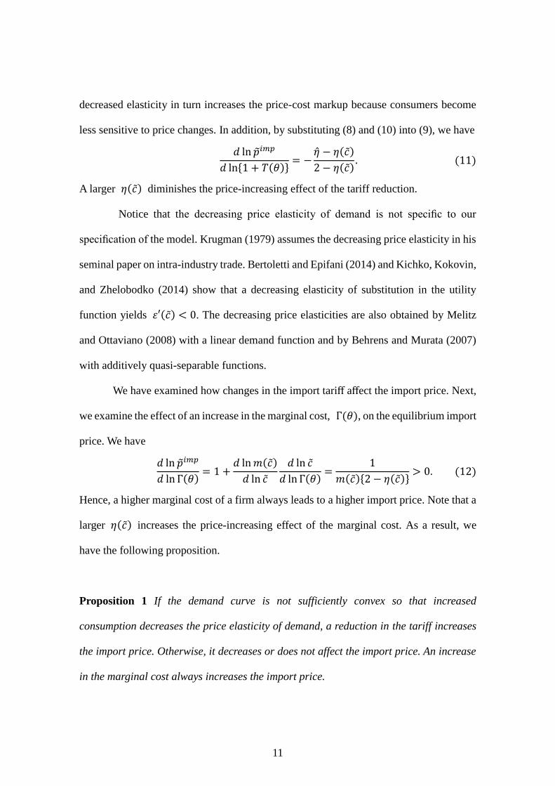
less sensitive to price changes. In addition, by substituting (8) and (10) into (9), we have
𝑑 ln 𝑝𝑖𝑚𝑝
𝑑 ln{1 + 𝑇(𝜃)}= −
�̂� − 𝜂(�̃�)
2 − 𝜂(�̃�). (11)
A larger 𝜂(�̃�) diminishes the price-increasing effect of the tariff reduction.
Notice that the decreasing price elasticity of demand is not specific to our
specification of the model. Krugman (1979) assumes the decreasing price elasticity in his
seminal paper on intra-industry trade. Bertoletti and Epifani (2014) and Kichko, Kokovin,
and Zhelobodko (2014) show that a decreasing elasticity of substitution in the utility
function yields ′(�̃�) < 0. The decreasing price elasticities are also obtained by Melitz
and Ottaviano (2008) with a linear demand function and by Behrens and Murata (2007)
with additively quasi-separable functions.
We have examined how changes in the import tariff affect the import price. Next,
we examine the effect of an increase in the marginal cost, Γ(𝜃), on the equilibrium import
price. We have
𝑑 ln 𝑝𝑖𝑚𝑝
𝑑 ln Γ(𝜃)= 1 +
𝑑 ln 𝑚(�̃�)
𝑑 ln �̃�
𝑑 ln �̃�
𝑑 ln Γ(𝜃)=
1
𝑚(�̃�){2 − 𝜂(�̃�)}> 0. (12)
Hence, a higher marginal cost of a firm always leads to a higher import price. Note that a
larger 𝜂(�̃�) increases the price-increasing effect of the marginal cost. As a result, we
have the following proposition.
Proposition 1 If the demand curve is not sufficiently convex so that increased
consumption decreases the price elasticity of demand, a reduction in the tariff increases
the import price. Otherwise, it decreases or does not affect the import price. An increase
in the marginal cost always increases the import price.

12
Proposition 1 provides an important implication for the impact of FTA utilisation
on import prices. By utilising an FTA scheme, a firm on one hand faces an FTA tariff that
is lower than the MFN tariff (the tariff effect). On the other hand, the firm must incur the
costs of meeting the RoO, part of which increases the marginal cost of the firm and thus
the import price (the RoO effect). If the demand curve is not extremely convex, the tariff
effect is more likely to increase the import price, while the RoO effect is less likely to
increase the import price. If the demand curve is more convex, however, the tariff effect
is less likely to increase (or will even decrease) the import price, while the RoO effect is
more likely to increase the import price. This implies that, if an FTA utilisation increases
the import price, the increased markup is the main driving force when the demand curve
is not extremely convex, while the RoO effect plays an important role when the demand
curve is more convex. In other works, if the RoO effect is not so significant, the firm gains
more and consumers gain less from FTA utilisation in the former case, while a large part
of the gains goes to consumers in the latter case.
We have shown that several exogenous parameters govern the equilibrium import
price. However, we cannot explicitly solve the equilibrium import price from (7), because
the price elasticity of demand that affects 𝑝𝑖𝑚𝑝 is not constant and varies with �̃�, which
recursively depends on the level of 𝑝𝑖𝑚𝑝. Hence, we implicitly define the import price
function as
𝑝𝑖𝑚𝑝 = 𝑓(𝑇(𝜃), Γ(𝜃), 𝐿). (13)
The effects of Γ(𝜃) on the import price are positive, while those of 𝑇(𝜃) and L depend
on the shape of the demand curve. If the demand curve is less convex and satisfies �̂� >
𝜂(�̃�), 𝑇(𝜃) and L have negative impacts on 𝑝𝑖𝑚𝑝. If the demand curve is highly convex

13
and satisfies 𝜂(�̃�) > �̂�, 𝑇(𝜃) and L have positive impacts on 𝑝𝑖𝑚𝑝.11 This equation is
estimated in the following empirical sections.
1.3. Choice between FTA and MFN Schemes
In this last subsection, we investigate a firm’s choice between an FTA scheme and
an MFN scheme. By substituting (7) into (4), the equilibrium operating profit of the firm
is given by
�̃�(�̃�, 𝜃) = [𝑚(�̃�) − 1]Γ(𝜃)�̃�𝐿. (14)
By differentiating (14) with respect to �̃�, we have
𝑑 ln �̃�(�̃�, 𝜃)
𝑑 ln �̃�= 1 +
𝑚(�̃�)
𝑚(�̃�) − 1
𝑑 ln 𝑚(�̃�)
𝑑 ln �̃�= 𝑚(�̃�){2 − 𝜂(�̃�)} > 0. (15)
Then, by differentiating (14) with respect to Γ(𝜃), and using (10) and (15), we can
confirm that an increase in the marginal cost reduces the firm’s operating profit:
𝑑 ln �̃�(�̃�, 𝜃)
𝑑 ln Γ(𝜃)= 1 +
𝑑 ln �̃�(�̃�, 𝜃)
𝑑 ln �̃�
𝑑 ln �̃�
𝑑 ln Γ(𝜃)= −{ (�̃�) − 1} < 0. (16)
Similarly, the effect of tariffs on the profit is given by
𝑑 ln �̃�(�̃�, 𝜃)
𝑑 ln{1 + 𝑇(𝜃)}=
𝑑 ln �̃�(�̃�, 𝜃)
𝑑 ln �̃�
𝑑 ln �̃�
𝑑 ln{1 + 𝑇(𝜃)}= − (�̃�) < 0. (17)
Based on these derivatives, we discuss the situation under which the producer of
each product variety chooses an FTA scheme over an MFN scheme. If the producer
chooses the FTA scheme, θ = 1 holds and the equilibrium price and the individual
consumption are respectively denoted by 𝑝𝐹𝑇𝐴 and 𝑐𝐹𝑇𝐴. Similarly, if it chooses the
MFN scheme, we have θ = 0, and the equilibrium price and the consumption are
respectively denoted by 𝑝𝑀𝐹𝑁 and 𝑐𝑀𝐹𝑁 . Substituting these prices and consumption
11 An increase in L decreases �̃�. Therefore, it decreases the import price if ′(�̃�) < 0 and increases
the import price if ′(�̃�) > 0.

14
into (14) yields the operating profit in each scheme:
𝜋𝐹𝑇𝐴 ≡ �̃�(𝑐𝐹𝑇𝐴, 1) = (𝑝𝐹𝑇𝐴 − 𝛿𝛾)𝑐𝐹𝑇𝐴𝐿 = {𝑚(𝑐𝐹𝑇𝐴) − 1}𝛿𝛾𝑐𝐹𝑇𝐴𝐿, (18)
𝜋𝑀𝐹𝑁 ≡ �̃�(𝑐𝑀𝐹𝑁 , 0) = (𝑝𝑀𝐹𝑁 − 𝛾)𝑐𝑀𝐹𝑁𝐿 = {𝑚(𝑐𝑀𝐹𝑁) − 1}𝛾𝑐𝑀𝐹𝑁𝐿. (19)
The difference between 𝜋𝐹𝑇𝐴 and 𝜋𝑀𝐹𝑁 is given by Δ𝜋 ≡ 𝜋𝐹𝑇𝐴 − 𝜋𝑀𝐹𝑁 .
First, we examine the tariff effect of FTA utilisation on the profit. Suppose δ = 1,
that is, the RoO do not raise the marginal cost and the FTA utilisation only lowers the
applied tariff from 𝑇𝑀𝐹𝑁 to 𝑇𝐹𝑇𝐴. From (17), we have Δ𝜋 > 0, meaning that the gain
in the operation profit from utilising the FTA is positive with δ = 1. Δ𝜋 becomes larger
as the tariff margin, 𝑇𝑀𝐹𝑁 − 𝑇𝐹𝑇𝐴, becomes larger. If the gain is high enough to exceed
the fixed cost of the FTA utilisation, Δ𝜋 > 𝐹, the firm chooses the FTA scheme over the
MFN scheme.
Next, we discuss the RoO effect of FTA utilisation. An increase in δ reduces 𝜋𝐹𝑇𝐴,
but does not affect 𝜋𝑀𝐹𝑁. From (16) and (18), we have
𝑑 ln Δ𝜋
𝑑 ln 𝛿=
𝜋𝐹𝑇𝐴
Δ𝜋
𝑑 ln 𝜋𝐹𝑇𝐴
𝑑 ln 𝛿= −
𝜋𝐹𝑇𝐴
Δ𝜋{ (𝑐𝐹𝑇𝐴) − 1} < 0. (20)
Therefore, as the RoO become more stringent, firms are less likely to utilise the FTA
scheme. In addition, a larger F obviously discourages FTA utilisation.
Finally, let us examine how a firm’s productivity affects the FTA utilisation.
Equation (16) tells us that an increase in γ reduces the firm’s profit. By comparing the
effect of γ on 𝜋𝐹𝑇𝐴 and 𝜋𝑀𝐹𝑁, we have
𝑑 ln Δ𝜋
𝑑 ln 𝛾= −{ (𝑐𝐹𝑇𝐴) − 1} +
𝜋𝑀𝐹𝑁
Δ𝜋{ (𝑐𝑀𝐹𝑁) − (𝑐𝐹𝑇𝐴)}. (21)
Given that Δ𝜋 > 0, the effect of γ on Δ𝜋 is always negative if (𝑐𝐹𝑇𝐴) > (𝑐𝑀𝐹𝑁)
holds, i.e. if the demand curve is sufficiently convex to satisfy 𝜂(�̃�) ≥ �̂� and ′(�̃�) > 0
holds. However, when the demand curve is not as convex (i.e. �̂� > 𝜂(�̃�)), the effect of γ
15
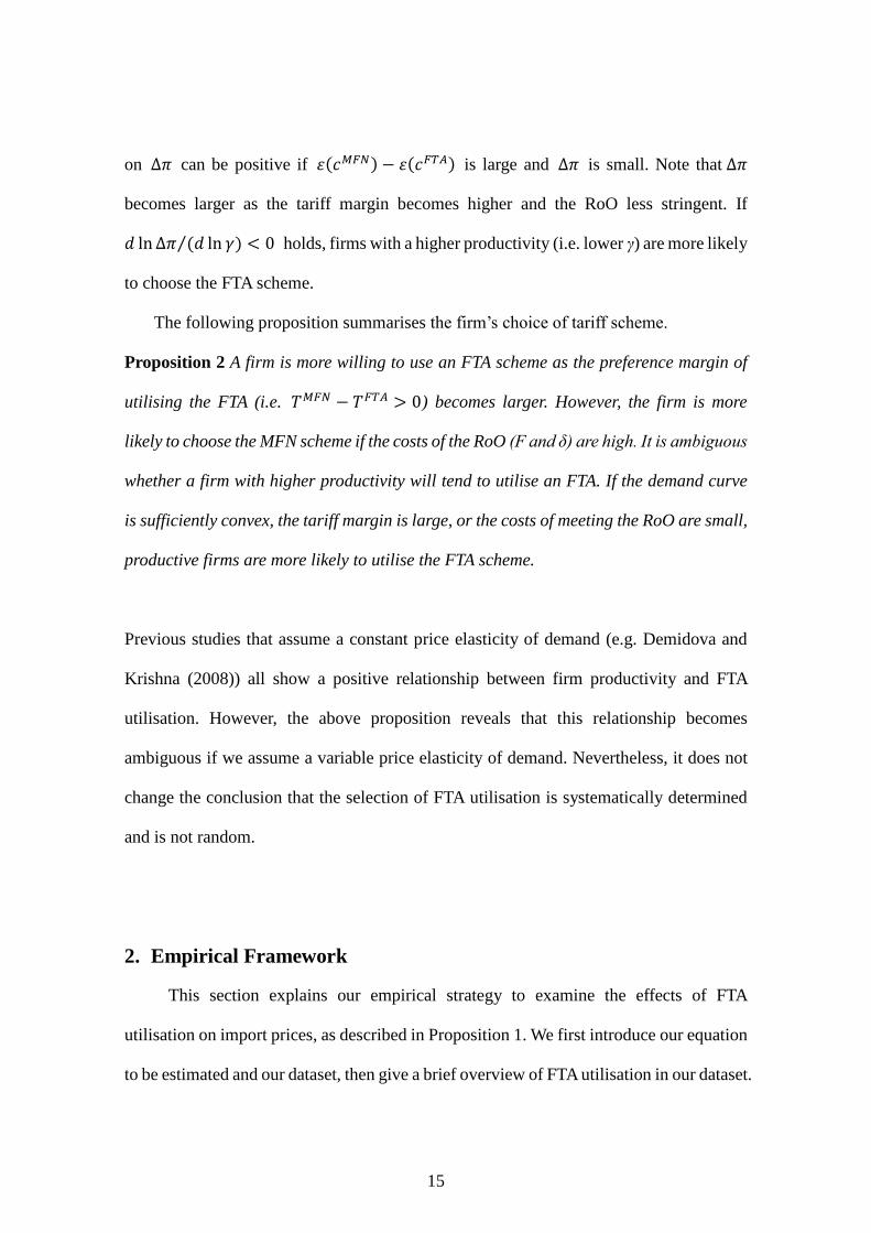
on Δ𝜋 can be positive if (𝑐𝑀𝐹𝑁) − (𝑐𝐹𝑇𝐴) is large and Δ𝜋 is small. Note that Δ𝜋
becomes larger as the tariff margin becomes higher and the RoO less stringent. If
𝑑 ln Δ𝜋 (𝑑 ln 𝛾)⁄ < 0 holds, firms with a higher productivity (i.e. lower γ) are more likely
to choose the FTA scheme.
The following proposition summarises the firm’s choice of tariff scheme.
Proposition 2 A firm is more willing to use an FTA scheme as the preference margin of
utilising the FTA (i.e. 𝑇𝑀𝐹𝑁 − 𝑇𝐹𝑇𝐴 > 0) becomes larger. However, the firm is more
likely to choose the MFN scheme if the costs of the RoO (F and δ) are high. It is ambiguous
whether a firm with higher productivity will tend to utilise an FTA. If the demand curve
is sufficiently convex, the tariff margin is large, or the costs of meeting the RoO are small,
productive firms are more likely to utilise the FTA scheme.
Previous studies that assume a constant price elasticity of demand (e.g. Demidova and
Krishna (2008)) all show a positive relationship between firm productivity and FTA
utilisation. However, the above proposition reveals that this relationship becomes
ambiguous if we assume a variable price elasticity of demand. Nevertheless, it does not
change the conclusion that the selection of FTA utilisation is systematically determined
and is not random.
2. Empirical Framework
This section explains our empirical strategy to examine the effects of FTA
utilisation on import prices, as described in Proposition 1. We first introduce our equation
to be estimated and our dataset, then give a brief overview of FTA utilisation in our dataset.

16
2.1. Specification
As mentioned in the introductory section, our main dataset is comprised of
transaction-level import data for Thailand from 2007 to 2011, obtained from the Customs
Department of Thailand.12 The dataset covers imports of all commodities for Thailand
and contains data on the customs clearing dates, HS eight-digit codes, exporting countries,
importing firm codes, firm branch codes, invoicing currencies, tariff schemes (e.g. FTA
or MFN), and import values in Thai baht. We classify the tariff schemes into three
categories: MFN schemes, FTA schemes, and other schemes. The other schemes include
imports under the schemes of bonded warehouses, free zones, investment promotion, duty
drawbacks under Section 19, and duty drawbacks for re-exports. 13 Although it is
interesting to take into account the choice of these other schemes, we do not include
imports under the other schemes in our sample, in order to keep our analysis simple.
During our sample period, Thailand had 10 FTAs, most of which overlap in country
coverage. Thailand had both bilateral and plurilateral FTAs with Japan, Australia, New
Zealand, and India. With other members of ASEAN, Thailand had six plurilateral FTA
schemes: ASEAN FTA, ASEAN-Australia-New Zealand FTA, ASEAN-China FTA,
ASEAN-Japan Comprehensive Economic Partnership, AKFTA, and ASEAN-India FTA.
In this paper, we define the following 15 countries as ‘FTA member countries’: Australia,
12 The data was collected confidentially. We have been given permission to use it for academic
purposes only. 13 Goods imported under the schemes of bonded warehouses, free zones, and investment promotion
may be exempted from the customs duties, subject to certain conditions. The duty drawback under
Section 19 or for re-exports enables exporting firms to obtain a refund on customs duty paid on
imported goods when those goods are used as an input for goods for export or are re-exported without
any transformation. Under these schemes, only firms with approval from the authorities in charge can
claim such privileges. Eligible imported goods and duty privileges vary among the schemes. For
example, virtually all goods imported under bonded warehouse and free zone schemes are duty-free.
Under the investment promotion scheme, raw materials are duty-free, while machinery may be either
duty-free or subject to a 50 percent tariff reduction. On the other hand, machinery is ineligible for a
refund on import duty paid under duty drawback schemes.

17
Brunei, Cambodia, China, India, Indonesia, Japan, Korea, Lao PDR, Malaysia,
Myanmar, New Zealand, Philippines, Singapore, and Viet Nam. Except for Korea, with
which Thailand concluded an FTA in 2010, all these countries have been FTA partner
countries for Thailand since at least the beginning of our sample period of 2007. Other
countries are defined as ‘FTA non-member countries’.
One empirical issue that needs attention when examining the effects of FTA
utilisation on import prices is that FTA utilisation and import prices are simultaneously
determined. Also, as shown in Proposition 2 in Section 2.3, the selection of FTA
utilisation is not random. Our identification strategy is the following. First, by taking
advantage of the nature of our transaction-level panel data, we conduct a difference-in-
differences (DID) analysis on the effects of FTA utilisation on import prices. To do so, in
addition to all FTA non-member countries, we include only one FTA member country,
Korea, as an exporting country. As mentioned, the FTA with Korea was the only one to
enter into force during our sample period (i.e. in 2010). Therefore, during 2007–2009, the
sample firms could not utilise an FTA scheme, but some were able to do so during 2010–
2011.
Second, another advantage of focusing on the AKFTA is that firms at the time were
not able to accurately predict when the FTA would enter into force. The ASEAN countries
and Korea began the FTA negotiations in 2003. However, the suspicion of illegal equity
trading by Prime Minister Thaksin Shinawatra and his family and the coup d’état by the
Royal Thai Army caused significant political turmoil in Thailand in 2006. As a result,
proceedings on various kinds of external economic policy, including FTA policy, stopped
in Thailand. As a result, the AKFTA was signed by Korea and the ASEAN member states,
with the exception of Thailand, in 2006. The AKFTA entered into force for all other

18
countries in either 2007 or 2008, but for Thailand it was unclear when or whether the
negotiations on AKFTA would restart. The agreement was finally signed in 2009 and
entered into force in 2010. This unpredictable situation of the AKFTA for Thailand due
to exogenous shocks to firms may enhance our identification for DID.14
Third, we examine establishment-level import prices rather than firm-level import
prices.15 We identify establishments by combining firm and branch identification codes.
Also, as mentioned, our sample’s exporting countries include FTA non-member
countries.16 These two notable characteristics of our dataset enable us to easily control
for all time-variant importing firm characteristics (e.g. productivity) in addition to fixed
effects with various dimensions. Namely, we can completely control for importing firm-
specific elements that affect both FTA utilisation and import prices.17 As a result, we use
the data on imports aggregated by importing firms, their branches, exporting countries,
HS eight-digit codes, tariff schemes, and years.
For empirical analysis, we parameterise the import price equation specified in (13).
In particular, we assume that it can be log-linearised as follows.
ln 𝑝𝑓𝑏𝑐𝑝𝑡 = 𝛼𝜃𝑓𝑏𝑐𝑝𝑡 − 𝛽 ln(1 + 𝑇𝑓𝑏𝑐𝑝𝑡) + 𝑢𝑓𝑏𝑐𝑝 + 𝑢𝑓𝑡 + 𝑢𝑐𝑠𝑡 + 𝑓𝑏𝑐𝑝𝑡, (22)
where
1 + 𝑇𝑓𝑏𝑐𝑝𝑡 = {1 + 𝑀𝐹𝑁𝑝𝑡 𝑖𝑓 𝜃𝑓𝑏𝑐𝑝𝑡 = 0
1 + 𝐹𝑇𝐴𝑝𝑡 𝑖𝑓 𝜃𝑓𝑏𝑐𝑝𝑡 = 1. (23)
pfbcpt denotes the import price (average unit value) by branch b of firm f for an HS eight-
14 As mentioned in the introductory section, another advantage of focusing on AKFTA is to avoid
firms’ complicated decisions on tariff schemes, which arise under the existence of multiple FTA
schemes. 15 We have greater firm-level variation if we examine transaction-level import prices, not the annual
average of import prices. 16 We also estimate our model for all exporting countries, including the other FTA member countries.
We will introduce the estimation result for this case later. 17 Instead of a model that controls for firm-specific elements, we also estimate a model that takes into
account to some extent the decision on FTA utilisation. The estimation results for this case are reported
in Table B1, Appendix B.

19
digit product p from country c in year t. θfbcpt indicates the tariff scheme and takes the
value one if an observation is based on an import under AKFTA, and zero otherwise
(called the ‘FTA dummy’). Tfbcpt is the tariff rate, which differs according to the tariff
scheme used for importing. MFN and FTA are the MFN rates and AKFTA preferential
rates, respectively. The coefficient α captures the RoO effect, i.e. δ in Section 2, while the
coefficient β is related to the tariff effect. As shown in Proposition 1, both coefficients are
expected to be positively estimated, particularly when the (inverse) demand curve is not
highly convex. Specifically, when an establishment starts to import product p under
AKFTA in year t, the magnitude of the tariff effect can be expressed as18
−𝛽{ln(1 + 𝐹𝑇𝐴𝑝𝑡) − ln(1 + 𝑀𝐹𝑁𝑝𝑡−1)} > 0. (24)
As mentioned, we control for various elements. ufbcp are the time-invariant,
importing establishment-exporting country-product fixed effects, which will control for
the importing establishment-product-specific inherent characteristics. uft are the time-
variant firm fixed effects used to control for all of the time-variant importing firm
characteristics. ucst are the time-variant, exporting country-sector fixed effects. We define
sectors by their HS two-digit level codes. The fixed effects will control for production
factor prices (e.g. wages) in the exporting countries, in addition to the sector-level demand
sizes (i.e. L in Section 2) or the degree of competition in the importing country, i.e.
Thailand. We expect that these various fixed effects control for elements that affect both
import prices and the tariff scheme choice.
As mentioned in the introductory section, our specification controls for biases that
were not controlled for in previous studies. The estimates of the product-level studies,
such as Cadot et al. (2005), Ozden and Sharma (2006), and Olarreaga and Ozden (2005),
18 Note that MFN rates are unchanged in 99.98 percent of all observations during our sample period.
20
include not only the effect of FTA utilisation but also the differences in exporter and/or
importer characteristics between FTA users and non-users. Our inclusion of time-variant
importing firm fixed effects controls for all of the importing firm characteristics, such as
firm productivity. Moreover, if importing firms do not change their country-product-level
trading partners frequently, our importing establishment-country-product dummy
variables will, to some extent, be able to control for exporting firm characteristics (e.g.
exporter productivity, 1/γ in Section 2).
The remaining noteworthy point is that some establishments import products from
Korea under both the MFN and FTA schemes. There are some possible reasons for this
use of multiple tariff schemes. One is that firms may import from different firms under
different tariff schemes (e.g. a productive export firm under the FTA scheme and a less
productive export firm under the MFN scheme). The other is that firms may make a
decision on the tariff scheme for each transaction and choose the FTA scheme for
transactions with a large trade value.19 For such observations, in the estimation sample,
we keep those importing under the FTA scheme but drop those importing under the MFN
scheme in order to control for exporter characteristics as much as possible through our
importing establishment (-product-country) fixed effects.20
19 Indeed, we find significant evidence that transactions with larger values are more likely to be under
FTA schemes. The results are shown in Table B2, Appendix B. 20 Imagine that establishment A imported a product from firms B and C under the MFN scheme in
2009, and again imported that product from firm B under the MFN scheme and from firm C under the
FTA scheme in 2010, although our dataset does not enable us to explicitly identify whether firms B
and C are different or not. In this example, we drop the observation of importing under the MFN
scheme in 2010, i.e. that of importing from firm B in 2010. Otherwise, our import establishment(-
product-country) dummy variable would take the value of one for two observations (i.e. two tariff
schemes) in 2010. To focus on the impacts of changing from the MFN to the FTA scheme, we drop
observations of importing under the MFN scheme for establishments that import products under both
the MFN and FTA schemes. As a result, in terms of the share of observations, 0.2 percent are dropped.

21
2.2. Data Overview
Before reporting our estimation results, we give an overview of AKFTA utilisation.
As mentioned, the AKFTA entered into force for Thailand in 2010 (signed in October
2009). Under the agreement, tariffs were reduced according to the category in which each
product is classified. The categories are normal track products, sensitive list products, and
highly sensitive list products. Since the tariff reduction for the products in the sensitive
and highly-sensitive lists started in 2012, AKFTA preferential rates are available only for
products placed in the normal track during our sample period after the enactment of
AKFTA (i.e. 2010 and 2011). The eligibility and level of the AKFTA preferential rates
did not change in 2010 or 2011. In both years, 70 percent of all tariff-line products (8,300
products) were eligible under the AKFTA. The average preferential margin, the difference
between the FTA and MFA rates, for the eligible products was approximately 12 percent.
The median and the maximum margins were 7 percent and 266 percent, respectively. The
most commonly applied RoO was for a ‘change in heading or regional value content’,
accounting for 77 percent of all tariff-line products. Other rules with a relatively high
share include ‘change in chapter or regional value content’ and ‘wholly-obtained’ (8%).21
Next, we give a brief overview of Thai imports from Korea. Table 1 reports various
statistics on Thai imports from Korea, including the number of importing establishment-
product observations, total import values, and the average import values at the importing
establishment-product level by year and tariff scheme. The left-hand panel shows the
statistics for the products with the same MFN rate as the FTA rate in 2011 and the right
panel shows those for products with a lower FTA rate than the MFN rate in 2011. Since
our sample FTA is a multilateral FTA (i.e. an FTA among Korea and 10 ASEAN member
21 More detailed statistics on the RoO and the preference margin are provided in Appendix A.

22
states) with cumulation rules, firms have incentives to use FTA schemes, even for
products with the same MFN rate as the FTA rate, as they can enjoy the benefits from
cumulation. When firms export their products to other AKFTA member countries, such
as Indonesia, under the AKFTA by using materials from Korea as inputs for their products,
those materials are imported under the AKFTA even if the MFN rate for those materials
is zero (see Hayakawa et al. [2013b]).
Table 1: Number of Importing Establishment-product Observations and Import
Values for Imports from Korea
MFN FTA Others MFN FTA Others
Number of importing establishment products
2007 11,073 4,116 19,467 6,589
2008 11,664 5,050 20,909 8,275
2009 9,902 3,406 19,287 5,942
2010 10,495 272 3,124 21,014 1,644 5,303
2011 11,162 302 3,084 22,513 2,218 5,585
Total import value (B million)
2007 58,916 53,549 34,880 38,418
2008 66,090 81,097 36,875 43,260
2009 53,738 63,628 27,298 41,251
2010 79,404 1,728 73,016 30,139 14,712 54,910
2011 79,165 1,662 62,478 31,372 29,719 46,138
Average import value (B million)
2007 5.3 13.0 1.8 5.8
2008 5.7 16.1 1.8 5.2
2009 5.4 18.7 1.4 6.9
2010 7.6 6.4 23.4 1.4 8.9 10.4
2011 7.1 5.5 20.3 1.4 13.4 8.3
MFN = FTA (# = 2,527) MFN > FTA (# = 5,773)
B = Thai baht, FTA = free trade agreement, LPM = linear probability model, MFN = most-favoured
nation.
Source: Customs Department, Thailand.
In this table, we focus on the right-hand panel, and define the products for which
the FTA rates are lower than MFN rates as ‘eligible products’. Taking a look at the number
of importing establishment-product observations, we can see that the number of FTA

23
users is small compared to the number of MFN users and importers under other schemes.
In particular, the number of MFN users is at least 10 times larger than that of FTA users.
However, total import values do not differ much between MFN and FTA users,
particularly for 2011. These observations imply that average imports at the importing
establishment-product level are much larger in FTA users than in MFN users, although
they are not so different between FTA users and the importers under other schemes. The
FTA users have nearly 10 times larger average import values than the MFN users. This
pattern is likely to reflect the qualitative differences in importing firms’ characteristics
between FTA users and MFN users.
Table 2 reports the changes in tariff schemes at the importing establishment-
product-level between 2007 and 2011. In the table, we restrict the sample products to
those in which FTA rates were lower than MFN rates in 2011. ‘Both’ indicates
observations for which an establishment imported a product under both the FTA and MFN
schemes. ‘None’ comprises cases of no imports under the MFN and FTA schemes, but
includes imports under other schemes. There are a large number of ‘only MFN’ users that
started or stopped importing. Each case accounts for more than 40 percent of the
observations. A relatively large number also started importing under only the FTA scheme.
The number of observations that changed from ‘MFN’ to ‘only FTA’ is the smallest,
accounting for 0.1 percent. This is even smaller than for the case of ‘both’ in terms of
numbers.

24
Table 2: Importing Establishment-product-level Changes in Tariff Scheme Status
for Imports from Korea, 2007–2011
None Only MFN Only FTA Both
Scheme in 2007
None Number 21,092 1,408 723
Share (%) 49 3 2
MFN Number 18,777 580 23 63
Share (%) 44 1.4 0.1 0.2
Scheme in 2011
FTA = free trade agreement, MFN = most-favoured nation.
Note: ‘Share’ indicates the share of the total observations.
Source: Customs Department, Thailand.
Table 3 reports the means and medians of the log-differences of importing
establishment-product-level changes in import prices (import unit values) from 2007 to
2011. In this table, we restrict the sample to observations that existed in both 2007 and
2011 and that used the MFN scheme in 2007. In the case of ‘both’, we calculated the price
changes for the MFN and FTA schemes separately. The ‘nominal’ row shows a relatively
large increase in import prices for observations that changed in status to ‘only FTA’. The
median also shows a positive change in observations that changed in status to the FTA
scheme under ‘both’. These results are unchanged when we deflate import prices using
the commodity-level consumer price index (normalised to 1 in 2007) obtained from the
Bureau of Trade and Economic Indices (Ministry of Commerce) of Thailand. The results
for real import price changes are shown in the row titled ‘real’. In sum, a relatively large
increase in import prices is observed for the products for which the status changed to
importing under the FTA scheme.

25
Table 3: Log-difference of Importing Establishment-product-level Import Prices
for Imports from Korea, 2007–2011
Only MFN Only FTA
MFN FTA
Nominal Mean -0.106 0.002 -0.285 -0.124
Median -0.064 0.022 -0.082 0.024
Real Mean -0.131 -0.003 -0.314 -0.153
Median -0.090 0.009 -0.144 0.004
Both
Scheme in 2011
FTA = free trade agreement, MFN = most-favoured nation.
Notes: The importing establishment-product observations are restricted to those for which the MFN
scheme was used in 2007. ‘Nominal’ indicates nominal price changes, while ‘real’ shows the change
in prices, deflated by the product-level consumer price index in Thailand.
Sources: Customs Department, Thailand; Bureau of Trade and Economic Indices (Ministry of
Commerce), Thailand.
3. Empirical Results
This section reports our estimation results on the effects of FTA utilisation on
import prices. We first present our basic estimation results to show how the results change
when we control for various importing firm-related fixed effects. Then, we report the
estimation results for equation (22). We also examine the role of some elements that are
not explicitly considered in Section 2. The basic statistics are provided in Table 4.
Table 4: Basic Statistics
Obs Mean Std. Dev. Min Max
ln Price 1,071,985 6.720 2.886 -11.575 20.976
FTA Dummy 1,071,985 0.003 0.051 0 1
ln (1+Tariff) 1,071,985 0.074 0.074 0 1.164
FTA Dummy * ln Total Imports 1,071,985 0.008 0.150 0 3.252
FTA Dummy * Preference Share 1,071,985 0.001 0.024 0 1
FTA Dummy * THB Invoice 1,075,739 0.000 0.004 0 1
FTA = free trade agreement, THB = Thai baht.
Note: ‘Total Imports’, ‘Preference Share’, and ‘THB Invoice’ are defined in Section 4.3.
Source: Authors’ computation.

26
3.1. Basic Estimation
Before estimating equation (22), we examine the existence or magnitude of the bias
in the estimation of the effects of FTA use on import prices when not controlling for
importing firm-related characteristics. To do so, we simply regress the log of import prices
on the FTA dummy variable by including only country-sector-year fixed effects. The
estimation result is reported in column (I) in Table 5. As in previous studies at the product
level, the coefficient for the FTA dummy is estimated to be significantly positive,
indicating that import prices were 12 percent higher in international transactions under
the FTA scheme than in those under the MFN scheme. Since, as was noted above, the
average reduction in tariff rates for the FTA scheme was 12 percentage points, this result
implies that, on average, the FTA tariff margins were absorbed by the increase in import
prices.
Table 5: Basic Estimation Results
(I) (II) (III)
FTA Dummy 0.110** 0.023 0.013
[0.051] [0.034] [0.039]
Country-Sector-Year FE YES YES YES
Importing Establishment-Country-Product FE NO YES YES
Importing Firm-Year FE NO NO YES
Number of obs 1,071,985 1,071,985 1,071,985
Adj R-squared 0.2863 0.8688 0.8719
FE = fixed effects, FTA = free trade agreement.
Notes: The dependent variable is the log of import prices at the importing establishment-country-
product-year level. ***, **, and * indicate 1%, 5%, and 10% significance, respectively. Robust
standard errors are in brackets.
Source: Authors’ computation.

27
The result changes significantly if we control for importing firm-related fixed
effects. Column (II) includes importing establishment-country-product fixed effects. The
coefficient for the FTA dummy is insignificant and its magnitude is greatly reduced. This
result implies that the estimates of the effect found in previous studies contain the inherent
characteristics of importing firms (establishments), which contributed to overestimation
of the effect. When controlling for not only importing establishment-country-product
fixed effects but also importing firm-year fixed effects, the coefficient is estimated to be
insignificant, as shown in column (III). Its magnitude is further reduced. Our findings
indicate that not only the inherent characteristics of importing firms but also the time-
variant characteristics resulted in overestimation in previous studies. In short, the effects
of FTA use on import prices are overestimated when not controlling for these importing
firm-related fixed effects.
3.2. Tariff and Rules of Origin Effects
Next, we estimate equation (22), which decomposes the effects of FTA utilisation
into tariff and RoO effects. Table 6 shows the results of the estimation, which control for
importing establishment-exporting country-product, importing firm-year, and exporting
country-sector-year fixed effects. In column (I), we include only the tariff rates, of which
the coefficient is estimated to be significantly negative. This result is consistent with the
theoretical prediction for the case of an insufficiently convex (inverse) demand curve, as
is demonstrated in Section 2. Namely, the tariff reduction resulting from the FTA
utilisation raises import prices. From the quantitative perspective, the average MFN and
AKFTA rates among eligible products are 12.8 percent and 0.8 percent, respectively.
Therefore, based on equation (24), the tariff effect contributes on average to raising import

28
prices by 3.6% (=−0.737*(0.0034−0.0525)*100). This rise implies that approximately
30% (=100*3.6/12.0) of the tariff margin is allocated to exporters based on the tariff effect.
Table 6: Tariff and Rules of Origin Effects
(I) (II)
FTA Dummy -0.075
[0.059]
ln (1+Tariff) -0.737* -1.374**
[0.391] [0.596]
Number of obs 1,071,985 1,071,985
Adj R-squared 0.8719 0.8719
FTA = free trade agreement.
Notes: The dependent variable is the log of import prices at the importing establishment-country-
product-year level. ***, **, and * indicate 1%, 5%, and 10% significance, respectively. Robust
standard errors are in brackets. All specifications include importing establishment-country-product,
importing firm-year, and sector-country-year fixed effects.
Source: Authors’ computation.
Column (II) of Table 6 includes both the FTA dummy and the tariff rate, which
respectively capture the RoO and tariff effects. The coefficient for the tariff rate is again
estimated to be significantly negative. Its absolute magnitude rises sharply from 0.737 to
1.374. A similar calculation as above indicates that, on average, the tariff effect raises
import prices by 6.7 percent and that approximately 56 percent of the tariff margin is
attributed to exporters. On the other hand, the coefficient for the FTA dummy is estimated
to be insignificant. These results are consistent with the theoretical demonstration in
Section 2.2., in that the tariff and RoO effects are more and less likely, respectively, to
raise import prices if the demand curve is not extremely convex. In short, on average, the
effects of FTA utilisation on import prices are mainly based on the tariff effect, not the
RoO effect. This implies that the effects of tariff reduction on import prices may be
indifferent between the cases based on FTA enactment and on multilateral liberalisation
(i.e. tariff reduction on the MFN basis).

29
We conduct some robustness checks.22 First, we estimate our model for the imports
from all countries, including those from other FTA member countries. We obtain
significant results for the FTA dummy and the tariff rate when introducing the variables
separately. In particular, the coefficient for the FTA dummy is estimated to be significantly
positive. However, the coefficient for the tariff rate is insignificant when introducing both
variables. Second, we use transaction-level data rather than aggregated data according to
the year. The results are similar to those in the first robustness check when introducing
the two variables separately, although the coefficient for the FTA dummy is negative when
introducing both variables. Third, in order to examine the differences in the RoO effect
across RoO, we introduce interaction terms of the FTA dummy variable with various
dummy variables indicating RoO. The results show that only the interaction term with the
regional value content rule is significantly negative. This sign is not consistent with our
expectation. Furthermore, the absolute magnitude of the coefficient is abnormally large.
3.3. Other Estimations
We also examine how the coefficient for the FTA dummy is related to some
elements not explored in our theoretical model. First, we consider the difference in the
bargaining power between an importer and an exporter in the determination of import
prices. Specifically, we examine the role of an importing firm’s size, since larger
importers are expected to have stronger bargaining power in price negotiation and may
thus curtail the extent of a price rise. To investigate this effect, we introduce an interaction
term of the FTA dummy with the importing firms’ total imports of all products from the
22 The results are shown in Tables B3–B5 in Appendix B. In Appendix B, we also report the estimation
results for the equations with an interaction term of the tariff variable with demand elasticity.

30
rest of the world (denoted by Total Imports). The use of importing firms’ total imports
rather than importing establishments’ total imports reduces the biases that arise from the
fact that importing establishments’ import prices and values are simultaneously
determined.
The results are shown in column (I) in Table 7. The coefficient for the FTA dummy
is estimated to be significantly positive. Its interaction term with the importing firm’s size
has a significantly negative coefficient. These results imply that, as is consistent with the
above expectation, the rise in import prices through the FTA utilisation is smaller when
the importer size is larger. From a quantitative perspective, since the average of the log
of total imports among AKFTA users is 2.913, the resulting magnitude of the FTA dummy
coefficient is −0.055 (=1.687−0.598*2.913). The additional rise in import prices is found
when trading under the AKFTA with importers that are smaller than the average size,
probably because of their weak bargaining power in price negotiation.
Second, we take the presence of competitors into account. The larger the number
of FTA users, including users of FTAs other than AKFTA, the smaller the advantage of
utilising the AKFTA scheme will be. In such a situation, importers may not allow
exporters to raise import prices by large percentages. To examine this effect, we introduce
an interaction term of the FTA dummy with the share of imports under all FTA schemes
in total imports for each tariff-line product (denoted by Preference Share). In the
computation of this variable, we do not include an establishment’s own imports (i.e. the
establishment’s imports of a given product from Korea). As reported in column (II), we
do not find a significant result for either the FTA dummy or its interaction term with
Preference Share.

31
Table 7: Other Estimations
(I) (II) (III)
FTA Dummy 1.687* -0.102 -0.089
[0.993] [0.072] [0.060]
FTA Dummy * ln Total Imports -0.598*
[0.338]
FTA Dummy * Preference Share 0.100
[0.128]
FTA Dummy * THB Invoice 0.376*
[0.212]
ln (1+Tariff) -1.327** -1.286** -1.510**
[0.598] [0.608] [0.604]
Number of obs 1,071,985 1,071,985 1,075,739
Adj R-squared 0.8719 0.8719 0.8721
FTA = free trade agreement, THB = Thai baht.
Notes: The dependent variable is the log of import prices at the importing establishment-country-
product-year level. ***, **, and * indicate 1%, 5%, and 10% significance, respectively. Robust
standard errors are in brackets. The specifications in columns (I) and (II) include importing
establishment-country-product, importing firm-year, and sector-year fixed effects. Column (III)
includes importing establishment-country-product-THB invoice, importing firm-year, and sector-
country-year fixed effects. ‘Total imports’ are the importing firms’ total imports of all products from
the rest of the world. ‘Preference share’ indicates the share of imports under all FTA schemes in total
imports for each tariff-line product. ‘THB invoice’ is a variable taking the value one if the invoicing
currency is the Thai baht, and zero otherwise.
Source: Authors’ computation.
Lastly, we introduce an interaction term between the FTA dummy and the invoicing
currency. The invoicing currency dummy variable is constructed so the dummy variable
takes the value one if the invoicing currency is in Thai baht (THB), i.e. the local currency,
and zero otherwise (denoted by THB Invoice). The literature has revealed that more
productive exporters, i.e. exporters with a higher market share, are more likely to choose
the local currency (i.e. the importing country’s currency) as an invoicing currency
(Devereux et al., 2015).23 Therefore, the interaction term may capture the effects of FTA
utilisation on import prices through the exporter’s characteristics. For this estimation, we
use data on imports aggregated by importing firm, their branches, HS eight-digit codes,
23 See also Asprilla et al. (2015) for several analyses on pricing-to-market.

32
tariff schemes, years, and the value of THB Invoice. Similarly, we introduce importing
establishment-country-product-THB Invoice indicator fixed effects. The results are shown
in column (III). While the FTA dummy has an insignificant coefficient, the coefficient for
its interaction with THB Invoice is estimated to be significantly positive. This finding
appears to indicate that productive exporters raise import prices, probably because of their
strong bargaining power in price negotiation.
4. Concluding Remarks
In this paper, we examined the impact of FTA use on import prices. For the analysis,
we employed establishment-level import data with information on the tariff scheme, the
FTA or MFN scheme, used for importing. Unlike previous studies in this literature, we
estimated the effects of FTA use on prices by controlling for the differences in importing
firm characteristics. Our main findings are as follows. First, the effect of FTA use on
import prices is overestimated when not controlling for importing firm-related fixed
effects. Second, the average effect of a tariff reduction based on FTA utilisation was a
3.6–6.7 percent rise in import prices. Third, in general, we did not find evidence of a price
rise due to the costs associated with RoO compliance. Fourth, we found several factors
that affect import prices. Specifically, importing firms with higher total import values are
found to reduce the rise of import prices. Also, the effect of FTA utilisation on import
prices is found to be larger for Thai baht invoiced transactions. These findings probably
reflect the difference in bargaining power between importers and exporters.
These results have the following implications. First, the rise in import prices through
FTA utilisation, accompanied by a fall in consumer prices, will become one of the sources

33
for welfare improvement, not only in importing countries but also in exporting countries.
This effect is based mainly on tariff reduction, which can be realised even in the case of
multilateral liberalisation (i.e. tariff reduction on the MFN basis). Although exporters
need to incur the additional costs of RoO compliance when utilising FTA schemes, these
costs are not passed through to export prices, and under such circumstances, exporting
countries may not enjoy additional welfare improvement. Second, the rise of import
prices becomes micro-level evidence for the benefit of the use of FTA schemes for
exporters. It is easy for policymakers to encourage importers to use FTA schemes because
importers can enjoy the visible benefits of saving tariff payments. On the other hand, the
benefits for exporters are not very clear because the use of FTAs requires documentation-
related work and procurement adjustments. According to our results, exporters are likely
to benefit from the use of FTAs because importers are likely to allow exporters to raise
export prices. Policymakers should encourage exporters to use FTA schemes by
explaining these benefits, in addition to the benefits resulting from increasing their
exports.
References
Amiti, M., O. Itskhoki, and J. Konings (2014), ‘Importers, Exporters, and Exchange Rate
Disconnect’, American Economics Review, 104(7), pp. 1942–1978.
Asprilla, A., N. Berman, O. Cadot, and M. Jaud (2015), ‘Pricing-to-Market, Trade Policy,
and Market Power’, Working Paper N IHEIDWP04-2015, Geneva, Switzerland:
The Graduate Institute of International and Development Studies.
Behrens, K. and Y. Murata (2007), ‘General Equilibrium Models of Monopolistic
Competition: A New Approach’, Journal of Economic Theory, 136(1), pp. 776–
787.
Berman, N., P. Martin, and T. Mayer (2012), ‘How Do Different Exporters React to
Exchange Rate Changes?’ Quarterly Journal of Economics, 127(1), pp. 437–492.

34
Bertoletti, P. and P. Epifani (2014), ‘Monopolistic Competition: CES Redux?’ Journal of
International Economics, 93(2), pp. 227–238.
Broda, J.G. and D. Weinstein (2006), ‘From Groundnuts to Globalization: A Structural
Estimate of Trade and Growth’, NBER Working Paper No. 12512, Cambridge, MA:
NBER.
Cadot, O., C. Carrere, J. de Melo, and A. Portugal-Perez (2005), ‘Market Access and
Welfare under Free Trade Agreements: Textiles under NAFTA’, World Bank
Economic Review, 19(3), pp. 379–405.
Cadot, O. and J. de Melo (2007), ‘Why OECD Countries Should Reform Rules of Origin’,
World Bank Research Observer, 23(1), pp. 77–105.
Cherkashin, I., S. Demidova, H. Kee, and K. Krishna (2015), ‘Firm Heterogeneity and
Costly Trade: A New Estimation Strategy and Policy Experiments’, Journal of
International Economics, 96(1), pp. 18–36.
Cirera, X. (2014), ‘Who Captures the Price Rent? The Impact of European Union Trade
Preferences on Export Prices’, Review of World Economics, 150(3), pp. 507–527.
Demidova, S. and K. Krishna (2008), ‘Firm Heterogeneity and Firm Behavior with
Conditional Policies’, Economics Letters, 98(2), pp. 122–128.
Devereux, M., B. Tomlin, and W. Dong (2015), ‘Exchange Rate Pass-through, Currency
of Invoicing and Market Share’, NBER Working Paper No. 21413, Cambridge,
MA: NBER.
Eaton, J., S. Kortum, and F. Kramarz (2011), ‘An Anatomy of International Trade:
Evidence From French Firms’, Econometrica, 79(5), pp. 1453–1498.
Feenstra, R. (1989), ‘Symmetric Pass-through of Tariffs and Exchange Rates under
Imperfect Competition: An Empirical Test’, Journal of International Economics,
27(1-2), pp. 25–45.
Feenstra, R. (2003), ‘Advanced International Trade: Theory and Evidence’, Princeton
University Press, Princeton.
Francois, J., B. Hoekman, and M. Manchin (2006), ‘Preference Erosion and Multilateral
Trade Liberalization’, World Bank Economic Review, 20(2), pp. 197–216.
Gorg, H., L. Halpern, and B. Muraközy (2010), ‘Why Do within Firm-product Export
Prices Differ across Markets?’ Kiel Working Paper No. 1596, Kiel, Germany: Kiel
Institute for the World Economy.
Hansen, B. (2000), ‘Sample Splitting and Threshold Estimation’, Econometrica, 68(3),
pp. 575–604.
Hayakawa, K. (2011), ‘Measuring Fixed Costs for Firms’ Use of a Free Trade Agreement:
Threshold Regression Approach’, Economics Letters, 113(3), pp. 301–303.
35
Hayakawa, K. (2014), ‘Does Firm Size Matter in Exporting and Using FTA Schemes?’
Journal of International Trade and Economic Development, 24(7), pp. 883–905.
Hayakawa, K., H.S. Kim, N. Laksanapanyakul, and K. Shiino (2013a), ‘FTA Utilization:
Certificate of Origin Data versus Customs Data’, IDE Discussion Papers 428,
Tokyo: Institute of Developing Economies.
Hayakawa, K., N. Laksanapanyakul, and K. Shiino (2013b), ‘Some Practical Guidance
for the Computation of Free Trade Agreement Utilization Rates’, IDE Discussion
Papers 438, Tokyo: Institute of Developing Economies.
Kee, H.L., L. Nicita, and M. Olarreaga (2008), ‘Import Demand Elasticities and Trade
Distortions’, Review of Economics and Statistics, 90(4), pp. 666–682.
Kichko S., S. Kokovin, and E. Zhelobodko (2014), ‘Trade Patterns and Export Pricing
under Non-CES Preferences’, Journal of International Economics, 94(1), pp. 129–
142.
Krugman, P.R. (1979), ‘Increasing Returns, Monopolistic Competition, and International
Trade’, Journal of International Economics 9(4), pp. 469–479.
Lawrence, R.Z. and D. Weinstein (1999), ‘Trade and Growth: Import-led or Export-led?
Evidence from Japan and Korea’, NBER Working Paper, No.7264, Cambridge,
MA: NBER.
Maddala, G.S. (1983), Limited-dependent and Qualitative Variables in Econometrics,
Cambridge, United Kingdom: Cambridge University Press.
Melitz, M. (2003), ‘The Impact of Trade on Intra-Industry Reallocations and Aggregate
Industry Productivity’, Econometrica, 71(6), pp. 1695–1725.
Melitz, M.J. and G.I.P. Ottaviano, (2008), ‘Market Size, Trade, and Productivity’, Review
of Economic Studies, 75(1), pp. 295–316.
Olarreaga, M. and C. Ozden (2005), ‘AGOA and Apparel: Who Captures the Tariff Rent
in the Presence of Preferential Market Access?’ The World Economy, 28(1), pp. 63–
77.
Ozden, C. and G. Sharma (2006), ‘Price Effects of Preferential Market Access: Caribbean
Basin Initiative and the Apparel Sector’, World Bank Economic Review, 20(2), pp.
241–259.
Takahashi, K. and S. Urata (2010), ‘On the Use of FTAs by Japanese Firms: Further
Evidence’, Business and Politics, 12(1), pp. 1469–3569.

36
Appendix A. AKFTA Basic Statistics
Table A1: Number and Share of RoO at the Tariff-line Level
Number of RoO Share of RoO (%)
CC 6 0.07
CC&RVC 13 0.16
CC/RVC 669 8.06
CH 17 0.2
CH&RVC 5 0.06
CH/RVC 6,394 77.04
CS/RVC 192 2.31
RVC 315 3.8
WO 689 8.3
Total 8,300 100 Notes: CC = change-in-chapter, CH = change-in-heading, CS = change-in-subheading, RoO = rules of
origin, RVC = regional value content, WO = wholly obtained rule. Source: Authors’ computation using the legal text of the AKFTA.
Figure A1: Distribution of the Preferential Margin in 2010/2011
Note: Products are restricted to those with a positive preference margin. Source: Authors’ computation using the legal text of the AKFTA.
0
.02
.04
.06
.08
De
nsity
0 100 200 300Preference margin (%)
kernel = epanechnikov, bandwidth = 1.7703

37
Appendix B. Other Estimation Results
In this appendix, we report some results of other estimations. Table B1 reports the
estimation results for the endogenous switching regression model in order to explicitly
incorporate firms’ decisions on tariff schemes into our empirical model.24 Specifically,
our model to be estimated is as follows.
𝜃𝑓𝑏𝑐𝑝𝑡 = 1 if 𝛾0 + 𝛾1 ln(1 + 𝑇𝑓𝑏𝑐𝑝𝑡) + 𝛾2 ln 𝑇𝐼𝑀𝑓𝑡 + 𝛾3 ln 𝑀𝑎𝑟𝑔𝑖𝑛𝑝𝑡 + 𝜖𝑓𝑏𝑐𝑝𝑡 > 0
𝜃𝑓𝑏𝑐𝑝𝑡 = 0 if 𝛾0 + 𝛾1 ln(1 + 𝑇𝑓𝑏𝑐𝑝𝑡) + 𝛾2 ln 𝑇𝐼𝑀𝑓𝑡 + 𝛾3 ln 𝑀𝑎𝑟𝑔𝑖𝑛𝑝𝑡 + 𝜖𝑓𝑏𝑐𝑝𝑡 ≤ 0
ln 𝑝𝑓𝑏𝑐𝑝𝑡 = 𝛽10 + 𝛽11 ln(1 + 𝑇𝑓𝑏𝑐𝑝𝑡) + 𝛽12 ln 𝑇𝐼𝑀𝑓𝑡 + 1𝑓𝑏𝑐𝑝𝑡 if 𝜃𝑓𝑏𝑐𝑝𝑡 = 1
ln 𝑝𝑓𝑏𝑐𝑝𝑡 = 𝛽20 + 𝛽21 ln(1 + 𝑇𝑓𝑏𝑐𝑝𝑡) + 𝛽22 ln 𝑇𝐼𝑀𝑓𝑡 + 2𝑓𝑏𝑐𝑝𝑡 if 𝜃𝑓𝑏𝑐𝑝𝑡 = 0
TIMft and Marginpt are the importing firm f’s total imports from the world in year t and
the AKFTA preference margin for product p in year t, respectively. The former variable
is introduced to control for time-variant importing firm characteristics. The latter variable
is one of the main variables in the selection equation, as shown in Proposition 2 in Section
2.3. The results are shown in column (I) in Table B1. As is consistent with the theoretical
discussion in Section 2, firms are more likely to utilise the AKFTA scheme when
importing products with a larger preference margin. As in the results of the FTA dummy
in Table 6, the constant term is not different between the FTA and MFN schemes and is a
little smaller in the FTA scheme. We also see significantly negative coefficients for tariff
rates and their quantitative difference between the FTA and MFN schemes. Notice that
these coefficients are based on the cross-product differences in tariff rates rather than the
over-time differences because the AKFTA rates do not change at all and the MFN rates
do not change in 99.98 percent of the observations during the sample period.
We also estimate this model by introducing a dummy variable that takes the value
one if the preference margin is greater than a certain cut-off level and zero otherwise,
24 As for the endogenous switching regression model, see Maddala (1983).

38
instead of a continuous variable of the margin. We estimate the model, changing the cut-
off level from 1 percent to the maximum level of our sample, i.e. 60 percent, by 1 percent
increments and find that log pseudo-likelihood becomes highest when the cut-off is set to
3 percent.25 This cut-off may be taken as the tariff equivalent rates of the FTA utilisation
cost. Indeed, 3 percent lies within the range of such rates found in previous studies.26 The
results when the cut-off is set to 3 percent are shown in column (II) and are qualitatively
unchanged with those in column (I).
In Table B2, we examine the determinants of AKFTA utilisation by employing
transaction-level data. Unlike the dataset used in the text, we do not aggregate according
to the year. The dependent variable is an indicator variable taking the value of one for
imports under the AKFTA scheme and zero for imports under the MFN scheme. Based
on the discussion in Section 2.3, independent variables are chosen. In particular, the
exporting firm-specific unit cost, i.e. the inverse of productivity, is negatively associated
with transaction values, as demonstrated in the following.
𝑑 ln 𝑝𝑖𝑚𝑝�̃�𝐿
𝑑 ln Γ(𝜃)=
𝑑 ln 𝑝𝑖𝑚𝑝
𝑑 ln Γ(𝜃)+
𝑑 ln �̃�
𝑑 ln Γ(𝜃)= −
(�̃�) − 1
𝑚(�̃�){2 − 𝜂(�̃�)}< 0.
We include tariff margin and transaction values as independent variables. Sample
observations are restricted to imports from Korea in 2010–2011. In columns (I) and (II),
we estimate the probit model, controlling for sector-year fixed effects to control for the
role of RoO. We obtain the natural results that the AKFTA is more likely to be chosen in
25 This grid search is based on the idea of the threshold regression model, which is proposed by
Hansen (2000). 26 For example, applying the threshold regression approach to the utilisation rate of Cotonou
preferences, Francois et al. (2006) found that the tariff equivalent costs of preference utilisation ranged
between 4 percent and 4.5 percent. Hayakawa (2011) also showed that by employing the threshold
regression method that the average tariff equivalent of fixed costs for use of an FTA for all existing
FTAs in the world is estimated to be around 3 percent. Cadot and de Melo (2007), in a survey article
on this literature, conclude that such fixed costs range between 3 percent and 5 percent of the product
price.
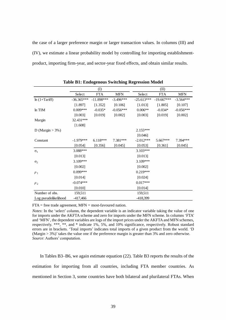
39
the case of a larger preference margin or larger transaction values. In columns (III) and
(IV), we estimate a linear probability model by controlling for importing establishment-
product, importing firm-year, and sector-year fixed effects, and obtain similar results.
Table B1: Endogenous Switching Regression Model
Select FTA MFN Select FTA MFN
ln (1+Tariff) -36.365*** -11.898*** -3.496*** -25.613*** -19.667*** -3.564***
[1.897] [1.352] [0.106] [1.013] [1.805] [0.107]
ln TIM 0.009*** -0.035* -0.056*** 0.006** -0.034* -0.056***
[0.003] [0.019] [0.002] [0.003] [0.019] [0.002]
Margin 32.431***
[1.608]
D (Margin > 3%) 2.155***
[0.046]
Constant -1.979*** 6.118*** 7.381*** -2.012*** 5.667*** 7.394***
[0.054] [0.356] [0.045] [0.053] [0.361] [0.045]
σ1 3.088*** 3.103***
[0.013] [0.013]
σ2 3.109*** 3.109***
[0.002] [0.002]
ρ 1 0.099*** 0.219***
[0.014] [0.024]
ρ 2 -0.074*** 0.017***
[0.010] [0.014]
Number of obs. 159,511 159,511
Log pseudolikelihood -417,466 -418,399
(I) (II)
FTA = free trade agreement, MFN = most-favoured nation.
Notes: In the ‘select’ column, the dependent variable is an indicator variable taking the value of one
for imports under the AKFTA scheme and zero for imports under the MFN scheme. In columns ‘FTA’
and ‘MFN’, the dependent variables are logs of the import prices under the AKFTA and MFN schemes,
respectively. ***, **, and * indicate 1%, 5%, and 10% significance, respectively. Robust standard
errors are in brackets. ‘Total imports’ indicates total imports of a given product from the world. ‘D
(Margin > 3%)’ takes the value one if the preference margin is greater than 3% and zero otherwise.
Source: Authors’ computation.
In Tables B3–B6, we again estimate equation (22). Table B3 reports the results of the
estimation for importing from all countries, including FTA member countries. As
mentioned in Section 3, some countries have both bilateral and plurilateral FTAs. When

40
constructing the FTA dummy, we do not distinguish between these FTAs, while the tariff
variable is constructed from the corresponding tariff scheme. We obtain significant results
for the FTA dummy and tariff rates when introducing those variables separately. In
particular, the coefficient for the FTA dummy is estimated to be significantly positive.
The coefficient for the tariff rate proves to be insignificant when introducing both
variables. In Table B4, we use transaction-level data. As in Table B2, we do not aggregate
according to year. The results are similar when introducing the two variables separately,
although the coefficient for the FTA dummy is negative when introducing both variables.
These results are unchanged, even when controlling for transaction-level values, as shown
in column (IV), though the transaction-level values and prices are simultaneously
determined.
Table B2: Selection of AKFTA Utilisation at the Transaction Level
(I) (II) (III) (VI)
Margin 3.934*** 6.447*** 0.224*** 0.224***
[0.042] [0.052] [0.022] [0.022]
ln Value 0.233*** 0.005***
[0.001] [0.000]
Method Probit Probit LPM LPM
Number of obs 884,967 884,967 862,327 862,327
Log pseudolikelihood -203,180 -177,294
Adj R-squared 0.803 0.8037
FTA = free trade agreement, LPM = linear probability model, MFN = most-favoured nation.
Notes: Observations are defined at the transaction level. The dependent variable is an indicator variable
taking the value of one for imports under the AKFTA scheme and zero for imports under the MFN
scheme. ***, **, and * indicate 1%, 5%, and 10% significance, respectively. Robust standard errors
are in brackets. The sample exporting country is restricted to Korea. The sample years are 2010–2011.
The probit model includes sector-year fixed effects. ‘LPM’ indicates a linear probability model and
includes importing establishment-product, importing firm-year, and sector-year fixed effects. ‘Value’
indicates import values while ‘margin’ is the difference between the MFN rates and the AKFTA rates.
Source: Authors’ computation.

41
The RoO effects might be different depending on the rule. Therefore, we introduce
interaction terms between the FTA dummy variable and various dummy variables
indicating the RoO. Specifically, we classify the RoO into the following five types and
their combinations based on ‘and’ (&) or ‘or’ (/): CC is change-in-chapter; RVC is
regional value content; CH is change-in-heading; CS is change-in-subheading; and WO
is wholly obtained rule. We set WO as the base rule. The results are reported in column
(I) in Table B5. The tariff rates again have a significantly negative coefficient. The
coefficient for the FTA dummy is insignificantly estimated, indicating that the RoO effect
does not exist when the RoO are WO. Also, most of the interaction terms have
insignificant coefficients. Only the interaction term with RVC is estimated to be
significantly negative. This sign is not consistent with our expectation. Furthermore, the
absolute magnitude of its coefficient is abnormally large.
These results are unchanged, even when we change the definition of the RoO and
the sample products. First, we define the RoO more broadly. Specifically, we classify CC,
CH, and CS into change-in-tariff classification (CTC). As shown in column (II), the
abnormal result in the interaction term of the FTA dummy with RVC is unchanged.
Second, the RoO effect should exist (if any) even when imported products are ineligible
for the AKFTA. Even in this case, importers still have an incentive to request exporters
to use FTA schemes in order to enjoy cumulation. Therefore, we also tried the estimation
by restricting sample products only to such ineligible products, in order to focus on the
effects of FTA utilisation other than the tariff effect. In this estimation, we do not include
a tariff rate variable because the MFN rates are unchanged in 99.98 percent of all
observations during our sample period. The effects of the tariff rates are absorbed by the
product fixed effects. As shown in column (III), we again obtain similar results for the

42
interaction terms with the RoO dummy variables.
Last, we examine the relationship between the tariff effect and demand elasticity. By
substituting equations (8) and (10) into (9), we have
𝑑 ln 𝑝𝑖𝑚𝑝
𝑑 ln{1 + 𝑇(𝜃)}= −
�̂� − 𝜂(�̃�)
2 − 𝜂(�̃�).
As (�̃�) becomes larger, �̂� = 1 + 1/ (�̃�) becomes smaller and 𝑑 ln 𝑝𝑖𝑚𝑝/[𝑑 ln{1 +
𝑇(𝜃)}] increases. This implies that the extent of the price-increasing effect of the tariff
reduction becomes smaller (or the price-decreasing effect of the tariff reduction becomes
larger) as the price elasticity of demand, (�̃�), increases. Therefore, introducing the
interaction term between tariff rates and the demand elasticity in Thailand (Demand
elasticity), we empirically investigate how demand elasticity affects the tariff effect. We
obtain the information on demand elasticity from Broda and Weinstein (2006) and Kee et
al. (2008), which provide the estimates at the HS three-digit level and at the HS six-digit
level, respectively.
Table B6 reports the estimation results. The results for the FTA dummy and tariff
variable are unchanged from those in Table 6. The coefficient for the interaction term is
estimated to be insignificant or significantly negative. This result is not consistent with
the above prediction. One important reason for this inconsistent result might be that the
estimates of demand elasticity are derived under the assumption of a constant price
elasticity of demand. However, as we demonstrated in Section 2, under the constant price
elasticity of demand, a change in the tariff rate does not affect the import price. Instead,
to obtain the significant tariff effect, we need to assume variable price elasticity of demand.
In sum, our result may indicate that the use of such estimates is not appropriate to examine
the relationship between the tariff effect and demand elasticity.

43
Table B3: Estimation Including Other FTA Member Countries as Exporters
(I) (II) (III)
FTA Dummy 0.042*** 0.038***
[0.008] [0.011]
ln (1+Tariff) -0.272*** -0.053
[0.067] [0.088]
Number of obs 2,343,542 2,343,542 2,343,542
Adj R-squared 0.8842 0.8842 0.8842
FTA = free trade agreement.
Notes: The dependent variable is the log of import prices at the importing establishment-country-
product-year level. ***, **, and * indicate 1%, 5%, and 10% significance, respectively. Robust
standard errors are in brackets. The sample exporting countries are all countries in the world, including
all FTA member countries. All specifications include importing establishment-country-product,
importing firm-year, and sector-year fixed effects.
Source: Authors’ computation.
Table B4: Estimation at the Transaction Level
(I) (II) (III) (IV)
FTA Dummy 0.028*** -0.079*** -0.282***
[0.010] [0.015] [0.016]
ln (1+Tariff) -0.553*** -1.083*** -1.056***
[0.098] [0.157] [0.137]
ln Value 0.370***
[0.000]
Number of obs 16,010,533 16,010,533 16,010,533 16,010,533
Adj R-squared 0.7451 0.7451 0.7451 0.7958
FTA = free trade agreement.
Notes: The dependent variable is the log of import prices at the transaction-level. ***, **, and *
indicate 1%, 5%, and 10% significance, respectively. Robust standard errors are in brackets. All
specifications include importing establishment-country-product, importing firm-year, and sector-year
fixed effects. Source: Authors’ computation.

44
Table B5: Decomposition of Rules of Origin Effects
(I) (II) (III)
FTA Dummy 0.111 0.136 0.442
[0.288] [0.287] [0.585]
FTA Dummy * CC/RVC -0.291
[0.276]
FTA Dummy * CH/RVC -0.174 -0.722
[0.266] [0.601]
FTA Dummy * CS/RVC 0.161 -0.612
[0.373] [0.611]
FTA Dummy * CH&RVC 0.215
[0.507]
FTA Dummy * RVC -1.050** -1.073** -1.764*
[0.463] [0.463] [0.911]
FTA Dummy * CTC/RVC -0.199
[0.264]
FTA Dummy * CTC&RVC 0.198
[0.507]
ln (1+Tariff) -1.299** -1.209*
[0.644] [0.642]
Base RoOs WO WO WO
Products All All Ineligible
Number of obs 1,071,985 1,071,985 315,636
Adj R-squared 0.8719 0.8719 0.8763
CC = change-in-chapter, CH = change-in-heading, CS = change-in-subheading, FTA = free trade
agreement, RVC = regional value content, WO = wholly obtained rule.
Notes: The dependent variable is the log of import prices at the importing establishment-country-
product-year level. ***, **, and * indicate 1%, 5%, and 10% significance, respectively. Robust
standard errors are in brackets. All specifications include importing establishment-country-product,
importing firm-year, and sector-year fixed effects. In this table, we interact the RTA dummy with
dummy variables indicating various RoO. ‘Ineligible’ in the category of products indicates that the
estimation sample products are restricted to those in which the AKFTA rates are same as the MFN
rates. Source: Authors’ computation.

45
Table B6: Tariff Effect and Demand Elasticity
BW KNO
FTA Dummy -0.077 -0.064
[0.060] [0.065]
ln (1+Tariff) -1.551** -1.458*
[0.727] [0.751]
ln (1+Tariff) * Demand elasticity 0.049 -0.102***
[0.115] [0.038]
Number of obs 1,062,859 985,482
Adj R-squared 0.872 0.8716
FTA = free trade agreement.
Notes: The dependent variable is the log of import prices at the importing establishment-country-
product-year level. ***, **, and * indicate 1%, 5%, and 10% significance, respectively. Robust
standard errors are in brackets. All specifications include importing establishment-country-product,
importing firm-year, and sector-country-year fixed effects. In column ‘BW’, we use the demand
elasticity obtained from Broda and Weinstein (2006). That of Kee et al. (2008) is used in column
‘KNO’. Source: Authors’ computation.

46
ERIA Discussion Paper Series
No. Author(s) Title Year
2016-24
Kazunobu HAYAKAWA
Nuttawut
LAKSANAPANYAKUL
Hiroshi MUKUNOKI
Shujiro URATA
Impact of Free Trade Agreement
Utilisation on Import Prices
Aug
2016
2016-23
Lili Yan ING, Olivier
CADOT and Janine
WALZ
Transparency in Non-tariff Meausres: An
International Comparison
Aug
2016
2016-22 VO Tri Thanh and
Cuong Van NGUYEN
Towards Responsive Regulatory
Management Systems: Country Report
for Viet Nam
July
2016
2016-21 Gilberto M. LLANTO Towards a Requisite Regulatory
Management System: Philippines
June
2016
2016-20 Lili Yan ING and
Olivier CADOT Facilitating ASEAN Trade in Goods
June
2016
2016-19
Doan Thi Thanh HA,
Kozo KIYOTA, and
Kenta YAMANOUCHI
Misallocation and Productivity:
The Case of Vietnamese Manufacturing
May
2016
2016-18
Vangimalla R. REDDY,
Shardendu K. SINGH
and Venkatachalam
ANBUMOZHI
Food Supply Chain Disruption due to
Natural Disasters: Entities, Risks, and
Strategies for Resilience
May
2016
2016-17
Arindam DAS-GUPTA,
Gemma B. ESTRADA,
Donghyun PARK
Measuring Tax Administration
Effectiveness and its Impact on Tax
Revenue
Apr
2016
2016-16 Naohiro YASHIRO Regulatory Coherence: The Case of Japan Mar
2016
2016-15 Song June KIM and Dae
Yong CHOI
Regulatory Coherence: The Case of the
Republic of Korea
Mar
2016

47
No. Author(s) Title Year
2016-14
Peter CARROLL,
Gregory BOUNDS and
Rex DEIGHTON-
SMITH
Towards Responsive Regulations and
Regulatory Coherence in ASEAN and
East Asia: The Case of Australia
Mar
2016
2016-13 Derek GILL Defining Regulatory Management System Mar
2016
2016-12 Derek GILL Regulatory Coherence: The Case of New
Zealand
Mar
2016
2016-11
Sang-Hyop LEE,
Jungsuk KIM and
Donghyun PARK
Demographic Change and Fiscal
Sustainability in Asia
Mar
2016
2016-10 Ayako OBASHI and
Fukunari KIMURA
The Role of China, Japan, and Korea in
Machinery Production Networks
Mar
2016
2016-09 Ayako OBASHI and
Fukunari KIMURA
Deepening and Widening Production
Networks in ASEAN
Mar
2016
2016-08 Willem THORBECKE
Increasing the Resilience of Asian Supply
Chains to Natural Disasters: The Role of
the Financial Sector
Feb
2016
2016-07
Hiroyuki NAKATA,
Yasuyuki SAWADA and
Kunio SEKIGUCHI
Market Concentration and Risk-
Prevention Incentives: The Case of the
Hard Disk Drive Industry
Feb
2016
2016-06 Meinhard BREILING
Tourism Supply Chains and Natural
Disasters: The Vulnerability Challenge
and Business Continuity Models for
ASEAN Countries
Feb
2016
2016-05
Masaru TANAKA and
Shigeatsu
HATAKEYAMA
Towards Reframing the Spirit of ASEAN
Environmentalism: Insights from Japan’s
COHHO Experience and Studies
Feb
2016
48
No. Author(s) Title Year
2016-04 Manaek SM PASARIBU
Challenges of Indonesian Competition
Law and Some Suggestions for
Improvement
Jan
2016
2016-03 VO Tri Thanh and
NGUYEN Anh Duong
Promoting Rural Development,
Employment, and Inclusive Growth in
ASEAN
Jan
2016
2016-02 Venkatachalam
ANBUMOZHI
Convergence of Opportunities:
Resilience and the ASEAN Community
Jan
2016
2016-01
Lili Yan ING, Shujiro
URATA and Yoshifumi
FUKUNAGA
How Do Exports and Imports Affect the
Use of Free Trade Agreements? Firm-
level Survey Evidence from Southeast
Asia
Jan
2016
Previous year of ERIA Discussion Paper, can be downloaded at:
http://www.eria.org/publications/discussion_papers/FY2015/
http://www.eria.org/publications/discussion_papers/FY2014/
http://www.eria.org/publications/discussion_papers/FY2013/
http://www.eria.org/publications/discussion_papers/FY2012/
http://www.eria.org/publications/discussion_papers/FY2011/
http://www.eria.org/publications/discussion_papers/FY2010/
http://www.eria.org/publications/discussion_papers/FY2009/
http://www.eria.org/publications/discussion papers/FY2008/


![8. [ERIA] Syok Pada Anak - Dr. Moh Supriatna](https://img.pdfslide.net/doc/110x75/5695d0c31a28ab9b0293c54b/8-eria-syok-pada-anak-dr-moh-supriatna.jpg)