Embed Size (px)
Citation preview
Impact of Geographic-Dependent Parameter Optimization on Climate Estimation andPrediction: Simulation with an Intermediate Coupled Model
XINRONG WU
NOAA/GFDL–Wisconsin Joint Visiting Program, Princeton, New Jersey, and South China Sea Institute of Oceanology,
Chinese Academy of Science, Guangzhou, and Key Laboratory of Marine Environmental Information Technology,
State Oceanic Administration, National Marine Data and Information Service, Tianjin, China
SHAOQING ZHANG
NOAA/GFDL, Princeton University, Princeton, New Jersey
ZHENGYU LIU
Center for Climate Research and Department of Atmospheric and Oceanic Sciences, University of Wisconsin—Madison,
Madison, Wisconsin, and Laboratory of Ocean–Atmosphere Studies, Peking University, Beijing, China
ANTHONY ROSATI AND THOMAS L. DELWORTH
NOAA/GFDL, Princeton University, Princeton, New Jersey
YUN LIU
Center for Climate Research and Department of Atmospheric and Oceanic Sciences,
University of Wisconsin—Madison, Madison, Wisconsin
(Manuscript received 14 October 2011, in final form 8 April 2012)
ABSTRACT
Because of the geographic dependence of model sensitivities and observing systems, allowing optimized
parameter values to vary geographically may significantly enhance the signal in parameter estimation. Using
an intermediate atmosphere–ocean–land coupled model, the impact of geographic dependence of model
sensitivities on parameter optimization is explored within a twin-experiment framework. The coupled
model consists of a 1-layer global barotropic atmosphere model, a 1.5-layer baroclinic ocean including
a slab mixed layer with simulated upwelling by a streamfunction equation, and a simple land model. The
assimilation model is biased by erroneously setting the values of all model parameters. The four most
sensitive parameters identified by sensitivity studies are used to perform traditional single-value pa-
rameter estimation and new geographic-dependent parameter optimization. Results show that the new
parameter optimization significantly improves the quality of state estimates compared to the traditional
scheme, with reductions of root-mean-square errors as 41%, 23%, 62%, and 59% for the atmospheric
streamfunction, the oceanic streamfunction, sea surface temperature, and land surface temperature, re-
spectively. Consistently, the new parameter optimization greatly improves the model predictability as a
result of the improvement of initial conditions and the enhancement of observational signals in optimized
parameters. These results suggest that the proposed geographic-dependent parameter optimization scheme
may provide a new perspective when a coupled general circulation model is used for climate estimation and
prediction.
Corresponding author address: Xinrong Wu, NOAA/Geophysical Fluid Dynamics Laboratory, 201 Forrestal Road, Princeton, NJ
08542.
E-mail: [email protected]
3956 MONTHLY WEATHER REV IEW VOLUME 140
DOI: 10.1175/MWR-D-11-00298.1
� 2012 American Meteorological SocietyUnauthenticated | Downloaded 02/06/22 07:06 AM UTC
1. Introduction
Because of its potential role in the reduction of model
bias and the improvement of climate predictability, pa-
rameter estimation for a coupled climate model is emerg-
ing as an important area of research. Traditional coupled
data assimilation uses observations to adjust state variables
only [called state estimation only (SEO)]. Therefore, the
generated climate states usually exhibit a systematic error
(Dee and Da Silva 1998; Dee 2005). The systematic error
in state estimation could lead model predictions to drift
toward imperfect model climate (Smith et al. 2007).
Based on the data assimilation theory (e.g., Jazwinski
1970), parameter estimation (e.g., Banks 1992a,b;
Anderson 2001; Hansen and Penland 2007) can be re-
alized by the state vector augmentation technique that
adds model parameters into control variables of data
assimilation. Many efforts have been made to advance
parameter estimation. Early studies focused on the four-
dimensional variational method (e.g., Navon 1997; Zhu
and Navon 1999). Their results showed that initial con-
ditions dominate short-term forecasts while longer
time-scale signals rely more on the positive impact of
optimized parameters. Based on ensemble Kalman filter
(EnKF; Evensen 2006), Annan and Hargreaves (2004)
applied parameter estimation in a highly nonlinear
model. Annan et al. (2005) estimated the parameters
of an intermediate complexity climate model using
EnKF.Aksoy et al. (2006a) investigated the performance
of EnKF through parameter estimation for the fifth-
generation Pennsylvania State University–National Cen-
ter for Atmospheric Research (PSU–NCAR) Mesoscale
Model (MM5) and found that with high-level model
sensitivities and covariances between parameters and
model states, parameters being estimated converged to
true value sufficiently. Similarly, Aksoy et al. (2006b)
applied the method to a two-dimensional sea-breeze
model and confirmed that simultaneous multiple-
parameter estimation can reduce the model state errors
effectively. Kondrashov et al. (2008) carried out para-
meter estimation with an intermediate coupled model
using extended Kalman filter and found that estimating
both state variables and parameters produced much
better results than SEO. Tong and Xue (2008a,b) em-
ployed ensemble square root Kalman filter (Whitaker
and Hamill 2002) to implement simultaneous state and
parameter estimation in single-moment ice microphysics
schemes using radar observations. Their results demon-
strated that the ensemble-based parameter estimation
can correct model errors in microphysical parameteriza-
tion. Recently, a coupled data assimilation scheme with
enhancive parameter correction (DAEPC) is designed to
address how to obtain a signal-dominant state-parameter
covariance so as to effectively optimize coupled model
parameters using observations in different system com-
ponents (Zhang et al. 2012). The DAEPC has been
applied to a simple pycnocline prediction model to im-
prove model decadal predictions (Zhang 2011a,b).
In this study, based on the DAEPC method imple-
mented in the ensemble adjustment Kalman filter
(EAKF; Anderson 2001), the impact of geographically
varying optimized parameter values on climate estima-
tion and prediction is investigated using an intermediate
coupled model. The coupled model consists of a baro-
tropic atmosphere, a 1.5-layer baroclinic ocean, and a
simple land model. The assimilation model is biased by
erroneously setting the values of all model parameters.
By comparing the results of single-value parameter esti-
mation (SPE) and geographic-dependent parameter op-
timization (GPO) with single- and multiple-parameter
cases, we show the superiority of GPO in both climate
estimation and prediction.
After briefly describing the intermediate coupled
model, section 2 also gives a brief description for the
enhancive parameter correction scheme and experimen-
tal setup that will be used throughout the paper. Section 3
investigates the geographic dependence of model pa-
rameter sensitivities. Section 4 presents the geographic-
dependent parameter optimization scheme, and section 5
discusses the impact of GPO on ‘‘climate prediction.’’ A
summary and a general discussion are given in section 6.
2. Methodology
a. An intermediate coupled model
To clearly illustrate the impact of the geographic de-
pendence of model sensitivities on parameter optimiza-
tion and avoid the complexity of a coupled general
circulationmodel (CGCM), an intermediate atmosphere–
ocean–land coupled model is first developed here. The
coupling scheme follows the work of Liu (1993) where
a linear ocean–atmosphere coupled model is designed to
study the interannual-scale feedbacks of the atmosphere
and ocean in extratropics. In this study, a vorticity ad-
vection equation is used to represent the atmosphere to
account the nonlinearity of the atmosphere. The atmo-
sphere is coupled with a 1.5-layer ‘‘baroclinic’’ ocean in-
cluding a slab mixed layer and simulated upwelling
through an oceanic streamfunction equation. To provide
a complete bottom boundary condition for the atmo-
sphere, a simple land model in which the evolution of
land surface temperature is driven by atmosphere–land
fluxes is added to the coupled system. All three model
components adopt 64 3 54 Gaussian grid and are for-
warded by a leapfrog time stepping with a half-hour in-
tegration step size. AnAsselin–Robert time filter (Robert
DECEMBER 2012 WU ET AL . 3957
Unauthenticated | Downloaded 02/06/22 07:06 AM UTC

1969; Asselin 1972) is introduced to damp spurious
computational modes in the leapfrog time integration.
1) THE ATMOSPHERE
The atmosphere is a global barotropic spectral model
based on the equation of potential vorticity conservation:
›q
›t1 J(c,q)5
�l(To 2mc) ocean surface
l(Tl 2mc) land surface, (1)
where q5by1=2c, b 5 df/dy, f denotes Coriolis pa-
rameter, y represents the northward meridional dis-
tance from the equator, c represents the geostrophic
atmosphere streamfunction, m is a scale factor that
converts streamfunction to temperature, l is the flux
coefficient from the ocean (land) to the atmosphere,
and To and Tl denote sea surface temperature (SST)
and land surface temperature (LST), respectively.
The terms at the right-hand side simulate the fluxes
from ocean and land, serving as the forcing of the atmo-
sphere. A 21 rhomboidal truncation is applied to trans-
form the grid values of c to spectral coefficients.
2) THE OCEAN
The ocean consists of a 1.5-layer baroclinic ocean with
a slab mixed layer (Liu 1993) and the simulated up-
welling by a streamfunction equation as
8>>><>>>:
›
›t
2
u
L20
!1b
›
›xu5 g=2c2Kq=
2u
›
›tTo 1 u
›To
›x1 y
›To
›y2Khu52KTTo 1AT=
2To 1 s(t, t)1Co(To 2mc)
, (2)
where u is the oceanic streamfunction; L20 5 g9h0/f 2, is
the oceanic deformation radius, with g9 and h0 being the
reduced gravity and mean thermocline depth; g denotes
momentum coupling coefficient between the atmo-
sphere and ocean; Kq is the horizontal diffusive co-
efficient of u; KT and AT are the damping coefficient
and horizontal diffusive coefficient, respectively, of
To; Kh 5KT 3 k3 f /g9 (Philander et al. 1984), repre-
senting the strength of upwelling (downwelling), and k
is the ratio of upwelling and damping. Because Eq. (2)
is more appropriate for extratropical ocean (Liu
1993), in order to enhance the high-frequent signal in
tropic, KT is set to be constant from 258N to the North
Pole and from 258S to the South Pole, and reduces
linearly toward the equator to 90% of the extratropical
value. The linearly varying damping coefficientKT acts
as a part of the ‘‘dynamic core’’ that does not engage in
parameter estimation. The quantity Co is the flux co-
efficient from the atmosphere to the ocean. The term
s(t, t) is the solar forcing that introduces the seasonal
cycle:
s(t, t)5KT 3 s0(t)3
�12
�1
4500t1
1
200
�
3 cos
�2p
t2 15
360
��, (3)
where s0 represents the annual-mean solar forcing with
zonal distribution, t denotes latitude, and t is the days at
the current time step. The period of solar forcing is set to
360 days, which defines the model calendar year.
3) THE LAND
The evolution of LST is simulated simply by a linear
equation:
m›
›tTl 52KLTl 1AL=
2Tl 1 s(t, t)1Cl(Tl 2mc) ,
(4)
where m represents the ratio of heat capacity between
the land and the ocean mixed layer; KL and AL are
damping and diffusive coefficients of Tl, respectively;
and Cl denotes the flux coefficient from the atmosphere
to the land.
It should be noted that because of our barotropic
representation of the atmosphere, it is more appropriate
to comprehend the coupling between the atmosphere
and the ocean and land in this system as a mathematical
way rather than a physical parameterization. However,
with the geographic distributions of synoptic and climate
prognostic variables, this model is sufficient in its math-
ematical complexity for our purpose to explore the im-
pact of the geographic dependence of model sensitivities
on parameter optimization.
4) PARAMETER CLASSIFICATION
Default values of all parameters are listed in Table 1.
The last 14 parameters are empirically determined by
trial-and-error tuning. Note that the solar forcing s(t, t)
will not alter once it is determined using the default
value of KT, so it also acts as a part of the dynamic core.
We define a vector b5 (l, m, h0, g,Kq, k,KT,AT, Co,m,
3958 MONTHLY WEATHER REV IEW VOLUME 140
Unauthenticated | Downloaded 02/06/22 07:06 AM UTC

KL, AL, Cl, h) as a collection of parameters, where h is
the Asselin–Robert time filtering coefficient. The bt
denotes the standard values of b in the ‘‘truth’’ model
that is used to produce ‘‘observations’’ (i.e., the samples
of the truth model states).
5) FEATURES AND VARIABILITY
We show the annual mean of model states and the
variability of To in this section. Starting from initial
conditions Z0 5 (c0, u0, T0o , T
0l ), where c0, u0, T0
o , and
T0l , zonal mean values of corresponding climatological
fields, the coupled model is run for 3050 years with bt.
Leaving the first 50 years as spinup period, what are
showing next is based on the data over the last 300 years.
Figure 1 shows the annualmean ofc (Fig. 1a),u (Fig. 1b),
To (Fig. 1c), and Tl (Fig. 1d). We can see the western
boundary currents, gyre systems, and the Antarctic
Circumpolar Current clearly. High-frequency signals
ofTo in the tropics are also described by themodel. The
time mean wave train pattern of the atmospheric stream-
function mainly exists in low and midlatitudes. Because
of the topography effect, the wave pattern in North
Hemisphere is more complicated than that in South
Hemisphere. For Tl, because of the weak coupling with
other components and the simple form of control equa-
tion, it basically takes a zonal distribution in the long time
mean. Note that the low temperature in tropical lands can
be attributed to the linear damping of KT in the solar
forcing.
To investigate the variability of To, we also apply
empirical orthogonal function (EOF) decomposition to
the time series of the 3000-yr anomalies (monthly mean).
Explained variances of the first six modes are 39%, 15%,
7%, 5%, 5%, and 4%, respectively. Time coefficients of
the first six modes are used to perform the power spec-
trum analysis to show the internal variability of To. The
characteristic time scales of the first sixmodes are 400, 50,
30, 10–20, 5–20, and 5–15 years, respectively (Fig. 2),
showing the nature of the model ocean variability with
multiple time scales (interannual to multicentennial).
b. Brief description of a coupled DAEPC
The details of DAEPC can be found in Zhang et al.
(2012), and here we only comment on a few aspects that
are related to this study. Following Zhang et al. (2012)
and Zhang (2011a,b), the EAKF (Anderson 2001) is
used to perform the simultaneously state estimation and
parameter optimization in this study. EAKF is a se-
quential implementation of Kalman filter (Kalman
1960; Kalman and Bucy 1961) under an ‘‘adjustment’’
idea. While the sequential implementation provides
much computational convenience for data assimilation,
the EAKF maintains the nonlinearity of background
flows as much as possible (Anderson 2001, 2003; Zhang
and Anderson 2003). Based on the two-step EAKF
(Anderson 2003; Zhang and Anderson 2003; Zhang
et al. 2007), parameter estimation is a process similar to
multivariate adjustment in state estimation for a non-
observable variable. The first step that computes the
observational increment is identical to state estimation
[see Eqs. (2)–(5) in Zhang et al. (2007)]. The second
step that projects the observational increment onto
relevant parameters can be formulated as
Dbk,i5cov(b, yk)
s2k
Dyk,i . (5)
TABLE 1. Default values of parameters.
Parameter Meaning Value Nature of the value
r Radius of the earth 6.365 3 106 m Untunable constant
V Angular velocity of the earth 7.292 3 1025 rad s21 Untunable constant
g9 Reduced gravity 0.026 m s22 Untunable constant
l Flux coefficient of the atmosphere 223 s22 K21 Empirically tuning
m Scale factor 2.2 3 1027 m22 s K Empirically tuning
h0 Mean thermocline depth 500 m Empirically tuning
g Momentum coupling coefficient 1025 (100 days)21 Empirically tuning
Kq Diffusive coefficient of oceanic streamfunction 1025 Empirically tuning
k Ratio between upwelling and damping 1/6 K m21 Empirically tuning
KT Damping coefficient of SST 1 (180 days) 21 Empirically tuning
AT Diffusive coefficient of SST 104 m2 s21 Empirically tuning
Co Flux coefficient of the ocean 1028 K m22 Empirically tuning
m Ratio of heat capacity between the land and ocean 0.1 Empirically tuning
KL Damping coefficient of land temperature 1 (180 days) 21 Empirically tuning
AL Diffusive coefficient of land temperature 104 m2 s21 Empirically tuning
Cl Flux coefficient of the land 1028 K m22 Empirically tuning
h Asselin–Robert filter coefficient 0.01 Empirically tuning
DECEMBER 2012 WU ET AL . 3959
Unauthenticated | Downloaded 02/06/22 07:06 AM UTC

Here Dyk,i represents the observational increment of the
kth observation yk for the ith ensemble member; Dbk,i
indicates the contribution of the kth observation to the
parameter b for the ith ensemble member; cov(b, yk)
denotes the error covariance between the prior ensem-
ble of parameter and the model-estimated ensemble
of yk; and sk is the standard deviation of the model-
estimated ensemble of yk.
DAEPC (Zhang et al. 2012) is a modification of the
standard data assimilation with adaptive parameter
estimation (e.g., Kulhavy 1993; Borkar and Mundra
1999; Tao 2003). Since the successfulness of parameter
estimation entirely depends on the accuracy of the
state-parameter covariance (Zhang et al. 2012), and that
model parameters do not have any dynamically sup-
ported internal variability, the accuracy of the ensemble-
evaluated covariance is determinedby the accuracy of the
model ensemble simulating the intrinsic uncertainty of
the states for which the observations try to sample. In
DAEPC, parameter estimation is activated after state
FIG. 1. Annual mean of (a) atmospheric streamfunction (m2 s21), (b) oceanic streamfunction (m2 s21), (c) SST (K),
and (d) LST (K).
FIG. 2. Power spectrums of the first six modes of monthly averaged SST anomalies. Dashed lines represent 95%
confidence upper limits.
3960 MONTHLY WEATHER REV IEW VOLUME 140
Unauthenticated | Downloaded 02/06/22 07:06 AM UTC

estimation reaches a quasi-equilibrium (QE) where the
uncertainty of model states is sufficiently constrained by
observations so that the state-parameter covariance is
signal dominant. A norm of model state adjustments is
used to determine whether the state estimation has
reached a QE state (Zhang et al. 2012). Then parameters
are adjusted using Eq. (5). The updated parameters are
applied to the next data assimilation cycle, which further
refines the state estimation.
The inflation scheme of DAEPC based on model
sensitivities of parameters (Zhang et al. 2012; Zhang
2011a,b) is a particular aspect of DAEPC that is ex-
tremely important for the application of this study. It is
formulated as
~bl 5bl 1max
1,a0sl,0
slsl,t
!(bl 2bl) , (6)
where bl and ~bl represent the prior and the inflated en-
semble of the parameter bl; sl,t and sl,0 denote the prior
spreads of bl at time t and the initial time; a0 is a constant
tuned by a trial-and-error procedure; sl is the sensitivity
of the model state with regard to bl; and the overbar
represents the ensemblemean.Equation (6)means that if
the prior spread of bl is less than a0/sl times the initial
spread, it will be enlarged to this amount.
c. Design of ‘‘twin’’ experiment
Starting from Z0 described in section 2a(5), the truth
model is run for 101 years to generate time series of truth
with the first 50 years as the spinup period. Observa-
tions of model states are generated through adding
a Gaussian white noise that simulates observational
errors to the relevant true states of the remaining 51
years at specific observational frequencies. The stan-
dard deviations of observational errors are 106 m2 s21
for c, 100 m2 s21 for u, and 1 K for To and Tl, respec-
tively; while corresponding sampling frequencies are
6 h (for c), 1 day (for u, To, and Tl). In this study, the
observation locations of c are global randomly and
uniformly distributed with the same density of the
model grids, while the observation locations of u, To,
and Tl are simply placed at 58 3 58 global grid points
that start from 858S, 08 at the bottom-left corner to
858N, 3558E at the top-right corner. Following previous
studies (Zhang and Anderson 2003; Zhang et al. 2004;
Zhang 2011a,b; Zhang et al. 2012), the ensemble size is
set as 20 throughout this study.
To roughly simulate the real-world scenario in which
both the assimilation model and the assimilation initial
condition are biased relative to observations, in our as-
similation model, all parameters are set with the values
of 10% greater than their true values (bb 5 1.1bt).
Starting from Z0, the biased model is also spun up for
50 years to generate the biased initial model states Z1 5(c1, u1, T1
o , T1l ). Then the ensemble initial conditions of
c are produced by superimposing a Gaussian white
noise with the standard deviation of 106 m2 s21 on c1,
while u, To, and Tl are not perturbed. In addition, initial
standard deviations of four most sensitive parameters
(see section 3) to be optimized are set to 1% of relevant
biased values, while the other 10 biased parameters are
not perturbed. We denote the ensemble initial condi-
tions of the coupled model as P.
Starting from P, a 51-yr model ensemble control run
without any observational constraint (denoted as CTL)
and an SEO experiment are first performed. Then all
the parameter estimation experiments start after SEO
has performed one year where the state estimation has
reached its QE (Zhang et al. 2012).
Leaving another 3 years as the parameter estimation
spinup, all evaluation for assimilation schemes next are
based on the last 47-yr results. Table 2 lists observation-
adjusted model variables and observation-optimized
model parameters in the assimilation. Here, co, uo, Too ,
and Tol represent observations; c, u, To, and Tl denote
model states to be estimated; and m, g, KT, and KL are
parameters to be optimized.
Given that various time scales exist among component
models, the multivariate adjustment scheme is only
performed within the ocean component (see Table 2).
Because of the leapfrog time stepping, a two-time level
adjustment (Zhang et al. 2004) is applied for state esti-
mation. Additionally, in order to remove spurious cor-
relations caused by long distance, the distance factor
(Hamill et al. 2001; Zhang et al. 2007) is introduced into
the filtering (Hamill et al. 2001; Zhang et al. 2007). For
c and Tl, the impact radius of observations is set to
500 km; while for u and To, it is set to 1000 km 3 cos
[min(t, 60)], where t denotes the latitude of model grids.
3. Geographic dependence of model sensitivitieswith respect to parameters
In this section we first investigate the model sensitiv-
ities with respect to parameters. Here, the sensitivity
study is conducted for all 14 parameters with the as-
similation model.
TABLE 2. Observation-adjusted model variables and observation-
optimized model parameters in the assimilation.
co uo Too To
l
State estimation c u, To u, To
Parameter optimization m g KT KL
DECEMBER 2012 WU ET AL . 3961
Unauthenticated | Downloaded 02/06/22 07:06 AM UTC

The ensemble spread of a model prognostic variable
when a perturbation is added on a parameter is used to
evaluate the relevant sensitivities quantitatively.
For the lth parameter (say bl), draw 20 Gaussian
random numbers with the standard deviation being 5%
of the default value of bl to produce perturbations, while
the other 13 parameters remain unperturbed. Starting
from Z1, the assimilation model is forwarded up to 11
years. Model states are perturbed with the ensemble of
bl. Because of the relatively short time scale of the at-
mosphere, the sensitivities of c with respect to bl are
computed using time series of 0.5–1 year. For the ocean
and land, sensitivities are calculated with the results of
last 10 years. This process is looped for each parameter.
Figure 3 shows the time–space-averaged sensitivities
of c (Fig. 3a), u (Fig. 3b), To (Fig. 3c), and Tl (Fig. 3d)
with respect to 14 parameters. Here KT and KL are the
most sensitive parameters because they determine the
time scales of To and Tl so that a tiny perturbation can
cause a dramatic drift of To and Tl. As a return, the dif-
ferent To and Tl further change the fluxes from the ocean
(land) to the atmosphere by which the new curls of wind
stress change the ocean currents. Because of the weak
coupling with other components and the linear nature of
the control equation ofTl,KL dominates the sensitivity of
Tl. According to the weak sensitivities of To with respect
to k and Co, as well as the small magnitude of the ad-
vective term, the nonlinearity is also weak in the To
equation. Therefore, KT also plays a main role in the
sensitivity of To. For c and u, the second sensitive
parameters are m and g.
Figure 4 presents the geographic-dependent distri-
bution of time-averaged sensitivities of cwith respect to
m (Fig. 4a), u with respect to g (Fig. 4b), To with respect
to KT (Fig. 4c), and Tl with respect to KL (Fig. 4d). The
most sensitive areas of the atmospheric streamfunction
are, in order, theAntarctic Circumpolar Current system,
the Antarctic continent, and the high latitudes of the
Northern Hemisphere. The sensitivities of the oceanic
streamfunction mainly focus on western boundary cur-
rent systems and subtropical gyres. By contrast, the
Antarctic Circumpolar Current is the most sensitive re-
gion of To. Subtropical circulations in both hemispheres
are the most insensitive areas of To. The most insensitive
region of Tl is the Antarctic continent and not much
different sensitivity is found for other continents.
4. Geographic-dependent parameter optimization
In this section, based on information of geographic-
dependent model sensitivities, we extend the DAEPC
(Zhang et al. 2012) to implement geographic-dependent
FIG. 3. Time–space-averaged sensitivities of (a) the atmospheric streamfunction, (b) the oceanic streamfunction,
(c) SST, and (d) LSTwith respect to all parameters. The sensitivity is defined by the ensemble spread of a model state
variable induced by the perturbation of parameter.
3962 MONTHLY WEATHER REV IEW VOLUME 140
Unauthenticated | Downloaded 02/06/22 07:06 AM UTC

parameter optimization (GPO) that pursues a signifi-
cant signal enhancement in estimated parameter values.
Before parameter optimization starts, it should be en-
sured that model state reaches the quasi-equilibrium
(Zhang et al. 2012). Through computing the norm of
model state adjustments, the state estimation spinup
period can be roughly determined as one year. We first
examine a simple case that only estimates a single pa-
rameter using observations.
a. Single parameter GPO
From section 3, we choose KT, the most sensitive pa-
rameter, to perform the parameter optimization. Ob-
servations of To are used to optimizeKT (Table 2) while
the sensitivity of To with respect to KT serves as the
sensitivity of KT. We first introduce the traditional one
parameter SPE briefly.
1) TRADITIONAL ONE PARAMETER SPE
SPE assumes that KT has no geographic distribution.
Starting from P, SEO is performed during the first year
to reach the QE of model states. For each analysis step
in the later 50 years, c, u, To, and Tl are adjusted by
corresponding observations first (Table 2). Then all
available observations of To are used to adjust the en-
semble of KT sequentially using Eq. (5). Last, the up-
dated ensemble of KT engages in the model integration
until the next analysis step. The inflation scheme
[Eq. (6)] is introduced into parameter estimation so as
to avoid losing ensemble spread. Here, the sensitivity
of KT, sl, is also a single value that is simply the time–
space-averaged sensitivity of To with respect to KT
(Fig. 3c). Through several trial-and-error tests, a0 takes
the value 1.0.Additionally, upper and lower bounds (here
are 650% of the default value) are set to constrain the
adjustment so that ensemble of KT cannot drift far away
from the biased value.
Solid and dashed lines in Fig. 5 show the time series of
RMSEs of To for SEO and SPE, respectively. There is an
obvious spinup phase for parameter estimation. During
this period, the RMSE of SPE is even larger than SEO.
With 3-yr parameter estimation, the RMSEofTo reaches
a stable state. Since all observations of To are used to
estimate the single value of KT, adjustments of observa-
tions that locate at sensitive and insensitive areas may be
counteracted. In consequence, SPE is a parameter esti-
mation scheme in the global-averaged sense that does not
consider the geographic dependence of sensitivity suf-
ficiently. Figure 6c shows the spatial distribution of
RMSEs of To for SPE. Compared with SEO (Fig. 6b),
SPE reduces errors in most areas. No pronounced ame-
lioration, however, is found in most sensitive and in-
sensitive areas (check with Fig. 4c).
2) ONE PARAMETER GPO
In this subsection, we introduce the main idea of GPO.
It is known that uncertainties of parameters can be
transferred to model states through model integrating.
Therefore, themodel sensitivity is geographic dependent,
which may impact the signal in parameter estimation.
To estimateKT better, GPO introduces the geographic
dependence of sensitivity into parameter estimation.
Through localizing the parameter sensitivity sl and al-
lowing optimized parameter values to vary geograph-
ically, signals in covariance can be assimilated sufficiently
and optimal parameters can be obtained under local least
FIG. 4. The geographic-dependent distributions of time-averaged sensitivities of (a) the atmospheric stream-
function with respect to m, (b) the oceanic streamfunction with respect to g, (c) SST with respect toKT, and (d) LST
with respect to KL.
DECEMBER 2012 WU ET AL . 3963
Unauthenticated | Downloaded 02/06/22 07:06 AM UTC

squares frame. In addition, the introduced inflation
scheme [Eq. (6)] is also geographic dependent. On one
hand, for a small sl (insensitive area), the inflation
level is large, which enhances the signal-to-noise ratio
in the parameter–observation covariance. On the other
hand, for a large sl (sensitive place), the high sensitivity
can maintain a high signal-to-noise ratio and the small
inflation factor can also prevent the model blowing up
due to the excess inflation of the parameter ensemble.
Therefore, the inflation scheme further enhances the
signal in parameter optimization.
The following steps outline the main procedures of
GPO for the intermediate coupled model and the ide-
alized observing system:
d Step 1: Starting fromP, SEO is applied to the first year
to reach the quasi-equilibrium of model state.d Step 2: For each analysis step in the later 50 years:
d Step 2.1: Compute observational increments for
observations of c, u, To, and Tl.d Step 2.2: Perform the state estimation according
to Table 2.d Step 2.3: Compute prior spreads of KT for model
grids that fall into the specific influence scope of
observation, then inflate the ensemble of KT and
update it using the observational increment ofTo.d Loop Steps 2.1–2.3 until all observations have
been processed. Then for each model latitude do
the following:d Step 2.4: For each ensemble member of KT,
compute its zonal average, which is assigned to
all To model grids at current latitude.d Step 2.5: For each ensemble member of KT,
compute the mean of adjoining three latitudes,
then the mean value is assigned to all To model
grids at the current latitude.
d Step 3: Integrate themodel with the updated ensemble
of KT until the next analysis step.
Note that a0 in the inflation scheme is set to 1. The
geographic-dependent sensitivity of To with respect to
KT (see Fig. 4c) serves as the sl. During the optimization
of KT, in order to use as many as possible observations
FIG. 5. Time series of RMSEs of SST for SEO (solid line), tra-
ditional SPE (dashed line) that uses observations of SST to esti-
mateKT, and GPO (dotted line) that uses the same observations to
optimize the geographic-dependent KT. The small panel is the
zoomed out version of the large one which includes the first year’s
results. Note that parameter estimation (optimization) is activated
after 1-yr SEO. Here, results of free run (CTL) are not shown
because of the dramatic error.
FIG. 6. Spatial distributions of RMSEs (K) of SST for (a) CTL; (b) SEO; (c) SPE, which uses observations of SST to
estimate KT; and (d) GPO, which uses the same observations to optimize the geographic-dependent KT. Note that
(c) and (d) use the same shade scale.
3964 MONTHLY WEATHER REV IEW VOLUME 140
Unauthenticated | Downloaded 02/06/22 07:06 AM UTC
and considering the zonal trait of the sensitivity of To
with respect to KT (see Fig. 4c), grids that locate be-
tween 708S and 708N are influenced by observations
whose latitudes are less than 500 km away, while other
grids are adjusted by the observations whose latitudes
are less than 3000 km away. The goal of step 2.4 is to
eliminate the zonal gradient of KT, ›KT /›x. Figure 4c
indicates that the zonal gradient of sensitivity can be
neglected relative to the meridional gradient. Here,
a simply zonal average of the KT ensemble is employed.
Similarly, step 2.5 is used to smooth the meridional gra-
dient of KT ensemble. Apparently, the gradient smooth
scheme depends on the geographic dependence of
model sensitivities. In the real world, both model sen-
sitivities and the representation of observations are
geographic dependent, so the related gradient smooth
scheme and parameter optimize method will be modi-
fied correspondingly.
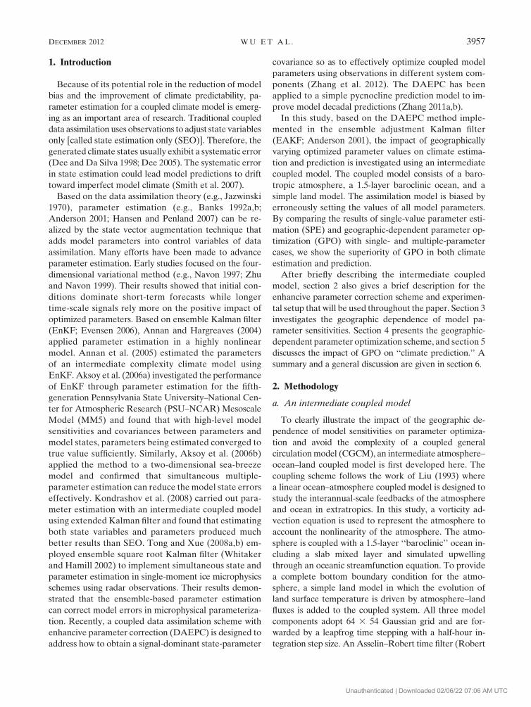
Table 3 lists the root-mean-square errors (RMSEs) of
all model components produced by different data as-
similation schemes we compare in this study. From first
four rows in Table 3, both SPE and GPO further reduce
errors of To greatly from SEO by 68% and 85%, re-
spectively, while SEO dramatically reduces the error of
To from CTL (by 96%). Note that because of the com-
putational modes induced by the inconsistent boundary
conditions between the SPE-produced SSTs (To) and
the SEO-produced LSTs (Tl) over the coastal regions,
the RMSEs of c and u for SPE and GPO are a little
larger than SEO. This means that it is very important for
all components to obtain a consistent observational
constraint in a coupled system. For Tl, because all three
schemes have the same KL and the seasonal cycles that
depend on the truth of KT, and the fact that KL and KT
are the two most sensitive parameters, the RMSE of Tl
for GPO is the same as that of SEO and SPE. Addi-
tionally, the weak and indirect coupling with To is also
a reason.
Figure 6d shows the spatial distribution of the RMSE
of To for GPO. Compared with CTL (Fig. 6a) and SEO
(Fig. 6b), significant improvements are made in global
areas. In addition, GPO significantly mitigates the error
in most sensitive and insensitive areas for SPE (Fig. 6c).
The dotted line in Fig. 5 shows the time series of RMSEs
of To for GPO, which indicates the smallest error of To
among all schemes after 3-yr parameter optimization
spinup period.
To present the advantage of GPO in detail, Fig. 7
shows the ensemble mean time series (the 10th year) of
To at an insensitive point (48.728N, 168.758E; top panel)
and a sensitive point (58.638S, 202.58E; bottom panel)
(see Fig. 4c). Dashed-dot, solid, dashed, and dotted lines
represent truth, SEO, SPE, and GPO, respectively.
Because of the global average meaning, SPE has no
significant improvement of To for these two grids com-
pared with SEO. For SEO, compared with truth, the
error of the sensitive point (bottom panel) is larger than
that of the insensitive point (top panel) because of the
high sensitivity. However, for GPO, as the explanation
at the beginning of section 4a(2), time series of To for
GPO significantly approach the truth. Evident un-
dulations exist in SEO, indicating the remarkable model
bias (here mainly stems from the uncertainty ofKT). For
TABLE 3. Total RMSEs of atmospheric streamfunction (c), oceanic streamfunction (u), SST (To), and LST (Tl) for all experiments.
c (m2 s21) u (m2 s21) To (K) Tl (K)
CTL 14 180 212.6 2557.08 31.89 30.08
SEO 977 499.2 89.71 1.20 3.68
Single-parameter SPE 1 023 025.8 91.15 0.39 3.68
Single-parameter GPO 1 083 616.7 91.44 0.18 3.68
Multiple-parameter SPE 864 313.1 81.00 0.47 2.79
Multiple-parameter GPO 510 321.2 62.12 0.18 1.15
FIG. 7. Two examples of ensemble mean time series (the 10th
year) of SST at (top) an insensitive point (48.728N, 168.758E) and(bottom) a sensitive point (58.638S, 202.508E). SPE uses observa-
tions of SST to estimate KT, and GPO uses the same observations
to optimize the geographic-dependent KT.
DECEMBER 2012 WU ET AL . 3965
Unauthenticated | Downloaded 02/06/22 07:06 AM UTC
SPE and GPO, however, the undulation is almost in-
visible, which confirms that the model bias has been
reduced sufficiently.
b. Multiple parameter
In a CGCM, usually there is an array of vital and sen-
sitive parameters. In this section we examine the general
case (i.e., multiple-parameter GPO). Here, the four most
sensitive parameters identified by the sensitivity study,
KT, KL, m, g, are chosen to perform simultaneously state
estimation and multiple-parameter GPO. Multiple-
parameter SPE is also conducted as an important refer-
ence. According to Table 2, observations of c, u, To, and
Tl are used to optimize m, g, KT, and KL, respectively.
Because model states have different sensitivities with re-
spect to various parameters, the single variable adjust-
ment is employed for simplicity. Again we first introduce
the traditional multiple-parameter SPE.
1) TRADITIONAL MULTIPLE-PARAMETER SPE
Similar to the one parameter case, SPE here assumes
that m, g, KT, and KL have no geographic distributions.
Starting fromP, with 1-yr SEO, for each analysis step in
the later 50 yr, state estimation is first performed the
same as SEO. Then all observations of c, u, To, and Tl
are used to, respectively, adjust ensembles of m, g, KT,
and KL. The updated parameter ensembles engage in
the next data assimilation cycle and act as prior pa-
rameter ensembles. The inflation scheme [Eq. (6)] is also
applied. Time–space-averaged sensitivities of c, u, To,
and Tl with respect to m, g, KT, and KL, respectively
(Fig. 3), are assigned to sl values of these four param-
eters.With trial-and-error tests, the related a0 values are
set to 106, 500, 1, and 0.2.
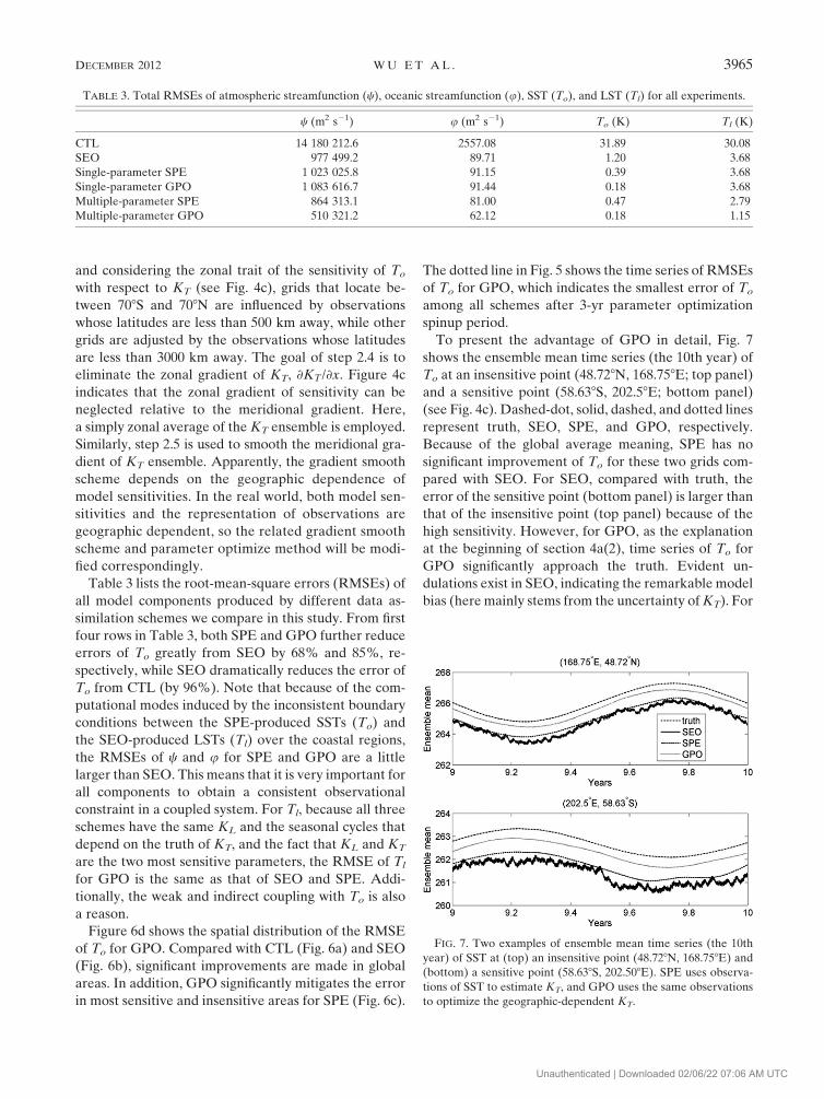
Blue and red lines in Fig. 8 show the time series of
RMSEs of c (Fig. 8a), u (Fig. 8b), To (Fig. 8c), and Tl
(Fig. 8d) for SEO and SPE, respectively. Significant
ameliorations are made for all model states. Improve-
ment levels of To and Tl are the most significant, which
results from the high sensitivities of KT and KL. From
total statistics in Table 3, RMSEs of c, u, To, and Tl are
reduced by 12%, 10%, 61%, and 24%, respectively,
from SEO to multiple-parameter SPE.
First and second columns in Fig. 9 display the spatial
distributions of RMSEs of c (Figs. 8a,b), u (Figs. 8d,e),
To (Figs. 8g,h), and Tl (Figs. 8j,k) for SEO (column 1)
and SPE (column 2). For Tl, according to Figs. 8j,k, SPE
reduces errors in almost all continents except the south
Antarctic continent. According to the spatial distribution
of sensitivity of Tl with respect to KL (see Fig. 4d), the
Antarctic continent is the only insensitive area. Because
SPE uses the global-averaged sensitivity and assumes
FIG. 8. Time series of RMSEs of (a) the atmospheric streamfunction, (b) the oceanic streamfunction, (c) SST, and
(d) LST for SEO (blue line); SPE (red line), which uses observations of the atmospheric streamfunction, the oceanic
streamfunction, SST, and LST to estimate m, g,KT, andKL, respectively; and GPO (green line), which uses the same
observations to optimize the geographic-dependent m, g,KT, andKL. Note that parameter estimation (optimization)
is activated after 1-yr SEO.
3966 MONTHLY WEATHER REV IEW VOLUME 140
Unauthenticated | Downloaded 02/06/22 07:06 AM UTC
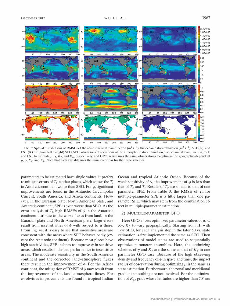
parameters to be estimated have single values, it prefers
tomitigate errors ofTl in other places, which causes theTl
in Antarctic continent worse than SEO. For c, significant
improvements are found in the Antarctic Circumpolar
Current, South America, and Africa continents. How-
ever, in the Eurasian plate, North American plate, and
Antarctic continent, SPE is even worse than SEO. As the
error analysis of Tl, high RMSEs of c in the Antarctic
continent attribute to the worse fluxes from land. In the
Eurasian plate and North American plate, large errors
result from insensitivities of c with respect to m there.
From Fig. 4a, it is easy to see that insensitive areas are
consistent with the areas where SPE behaves badly (ex-
cept the Antarctic continent). Because most places have
high sensitivities, SPE inclines to improve c in sensitive
areas, which results in the bad performance in insensitive
areas. The moderate sensitivity in the South America
continent and the corrected land–atmosphere fluxes
there result in the improvement of c. For the Africa
continent, the mitigation of RMSE ofcmay result from
the improvement of the land–atmosphere fluxes. For
u, obvious improvements are found in tropical Indian
Ocean and tropical Atlantic Ocean. Because of the
weak sensitivity of g, the improvement of u is less than
that of To and Tl. Results of To are similar to that of one
parameter SPE. From Table 3, the RMSE of To for
multiple-parameter SPE is a little larger than one pa-
rameter SPE, which may stem from the combination ef-
fect in multiple-parameter estimation.
2) MULTIPLE-PARAMETER GPO
Here GPO allows optimized parameter values of m, g,
KT, KL to vary geographically. Starting from P, with
1-yr SEO, for each analysis step in the later 50 yr, state
estimation is first implemented the same as SEO. Then
observations of model states are used to sequentially
optimize parameter ensembles. Here, the optimizing
schemes of g and KT are the same as that of KT in one
parameter GPO case. Because of the high observing
density and frequency of c in space and time, the impact
radius of observation during optimizing m is the same as
state estimation. Furthermore, the zonal and meridional
gradient smoothing are not involved. For the optimiza-
tion of KL, grids whose latitudes are higher than 708 are
FIG. 9. Spatial distributions of RMSEs of the atmospheric streamfunction (m2 s21), the oceanic streamfunction (m2 s21), SST (K), and
LST (K) for (from left to right) SEO; SPE, which uses observations of the atmospheric streamfunction, the oceanic streamfunction, SST,
and LST to estimate m, g, KT, and KL, respectively; and GPO, which uses the same observations to optimize the geographic-dependent
m, g, KT, and KL. Note that each variable uses the same color bar for the three schemes.
DECEMBER 2012 WU ET AL . 3967
Unauthenticated | Downloaded 02/06/22 07:06 AM UTC

impacted by the observations whose latitudes are less
than 3000 km away, while other grids are influenced by
the observations whose latitudes are less than 1000 km
away. The gradient smoothing is implemented for the
optimization of KL. Additionally, the geographic-
dependent distributions of the time-averaged sensitiv-
ities of c, u, To, and Tl with regard to m, g, KT, and KL
(see Fig. 4), respectively, serve as the relevant spatial sl
values. The a0 values of m, g,KT, andKL are set to 1.53106, 1000, 1, and 1.5, respectively.
The green line in Fig. 8 shows the time series of
RMSEs of c (Fig. 8a), u (Fig. 8b), To (Fig. 8c), and Tl
(Fig. 8d) for GPO. Relative to SEO (blue line) and SPE
(red line), all model states are improved significantly.
From the last two rows in Table 3, GPO reduces RMSEs
of c, u, To, and Tl by 41%, 23%, 62%, and 59%, re-
spectively, from multiple-parameter SPE.
The last column in Fig. 9 shows the spatial distribu-
tions of RMSEs of c (Fig. 9c), u (Fig. 9f), To (Fig. 9i),
and Tl (Fig. 9l) for GPO. For Tl, GPO reduces RMSEs
of SPE in all lands. However, Antarctic continent is still
worse than SEO (Fig. 9j), which may be caused by the
following two reasons. One lies in the fact that Tl is so
insensitive with respect to KL in this place (Fig. 4d) that
it needs a very large a0 to enhance the signal-to-noise
ratio of the error covariance. However, too large a0 may
blow up KL in other places. Therefore, it is difficult to
balance the insensitivity of Antarctic continent and the
sensitivities of other places only through coordinating
a0. Even so, GPO improves the Tl in the Antarctic
continent for SPE. The other is that there are too few
observations to constrain the ensemble of KL in that
place. Improvements ofTl in other places further correct
the fluxes from the land to the atmosphere. For c, relative
to SPE (Fig. 9b), significant improvements are made in
the Eurasian plate and North American plate, which
contributes to the localization of m and the improvement
of fluxes from the land to the atmosphere. There is also
FIG. 10. Variations of (a),(c) ACC and (b),(d) RMSEwith the forecast lead time of the forecasted ensemblemeans
of the (a),(b) atmospheric streamfunction and (c),(d) SST for SEO (solid line), SPE (dashed line), and GPO (dotted
line), which applies the global means of observation-optimized parameters into prediction model. The dashed line in
(a) represents the critical ACC value (0.6) of valid forecast time scale. The small panel is the zoomed out version of
(d), which shows the complete evolutions of RMSE of To for these three schemes.
3968 MONTHLY WEATHER REV IEW VOLUME 140
Unauthenticated | Downloaded 02/06/22 07:06 AM UTC

a pronounced amelioration in Antarctic continent,
which is consistent with the results of Tl. Compared with
SEO (Fig. 9a), GPO reduces RMSEs of c notably for
almost all places except the southernmost of Antarctic
continent, which is again in line with the result of Tl. For
u, the error level is reduced relative to both SPE and
SEO. Because of the improvements of both g and c,
forcings from the atmosphere are also corrected, which
further reduces the error of u. Results of To are nearly
the same as one parameter GPO.
5. Impact of GPO on ‘‘climate’’ prediction
To evaluate the impact of GPO on the model pre-
diction, 20 forecast initial conditions are selected every 2
years apart from analysis fields of 5–43 years for SEO,
multiple-parameter SPE, and multiple-parameter GPO.
Then 20 forecast cases are forwarded up to 10 years for
these three assimilation schemes. Note that in order to
eliminate the discrepancy of parameter structures in the
prediction model and the truth model, which produces
observations, the global mean value of each GPO-
generated parameter is applied to the prediction model.
Here, the global anomaly correlation coefficient (ACC)
of the forecasted ensemble mean is used to evaluate the
global pattern correlation verified with the truth, and an
ad hoc value of 0.6 ACC is employed to evaluate the
valid time scale of forecast (Hollingsworth et al. 1980);
the global RMSE of the forecasted ensemble mean is
used to evaluate the global absolute error relative to the
truth. However, in a CGCM with instrumental data, the
error of the innovation of forecasts to observations may
be a more appropriate quantity to evaluate forecast skills
of different data assimilation schemes (see e.g., Fukumori
et al. 1999).
a. Weather forecast skill
With the observation-estimated single-value parame-
ters, SPE extends the valid atmosphere forecast of SEO
from 8 to 10 days (see Fig. 10a). By comparison, with
better initial conditions (see the initial RMSE of c for
GPO in Fig. 10b) and global means of GPO-produced
parameters, GPO shows a smaller RMSE and a higher
ACC, which lead to a 13-day valid weather forecast time
scale. Note that GPOmixes with SPE after a lead time of
30 days, which is roughly the time scale of the predic-
tability of the atmospheric signals in this intermediate
coupled model.
b. Climate prediction skill
Because KT dominates the To equation, biased KT
in SEO makes the RMSE of To (see solid line in
Fig. 10d) increase rapidly and dramatically. With the
observation-estimated single-value KT and the global
mean of observation-optimized geographic KT, SPE
and GPO mitigate the RMSE of To significantly (see
dashed and dotted lines in Fig. 10d) while GPO shows the
least error of To. The erroneously set KT causes a low
initial ACC (0.36) (see the solid line in Fig. 10c) of the
SEO-generated initial condition.With the observation-
estimated single-valued KT, the initial ACC is improved
(0.48). but still not higher than 0.6. However, with the
geographic-dependent parameter optimization, the ini-
tial ACC is greatly enhanced (0.65). GPO maintains a
higher ACC than SPE for the first 3 years of lead time. It
seems that with the global mean of a GPO-generated
geographic-dependent parameter, the model has a supe-
rior performance compared to the case using a SPE-
produced parameter value. Note that when the method
is applied to a CGCM for climate estimation and pre-
diction with instrumental data, due to no truth parame-
ters existing, we shall directly apply the GPO-generated
parameters into the prediction model.
6. Summary and discussion
An intermediate atmosphere–ocean–land coupled
model is developed to investigate the impact of geo-
graphic dependence of model sensitivities on parameter
optimization. The coupled model consists of a barotropic
atmosphere, a 1.5-layer baroclinic ocean with a slab
mixed layer, and a simple land model. A biased twin-
experiment framework is designed by setting a 10%
overestimate error for all model parameters in the as-
similation model, while the ‘‘truth’’ model with standard
parameter values produces ‘‘observations.’’ Then, ob-
servations are assimilated into the assimilation model
to implement single-value parameter estimation and
geographic-dependent parameter optimization. Experi-
ments show that the new geographic-dependent pa-
rameter optimization substantially reduces the model
bias and improves the quality of climate estimation,
while the single-value parameter estimation cannot ef-
fectively extract observational information according to
geographically variant sensitivities. With better initial
conditions and signal-enhanced parameter values, the
geographic-dependent parameter optimization signifi-
cantly improves the model predictability.
Although many improvements have been shown with
the intermediate coupled model and the idealized ob-
serving system, several problems remain before applying
GPO to CGCMs. First, in a CGCM, besides model bias
induced by uncertainty of parameter, physical processes
also introduce complicated model biases. How the com-
plex model biases impact on GPO needs to be inves-
tigated further. Second, the real observation systems are
DECEMBER 2012 WU ET AL . 3969
Unauthenticated | Downloaded 02/06/22 07:06 AM UTC

geographic dependent, which directly impacts the signals
in parameter optimization. Using sparse observations in
a nonsensitive region will degrade the signal-to-noise
ratio of parameter optimization. Third, the constant a0 in
the inflation scheme is determined through trial-and-
error tests. In a CGCM, we may need to implement an
adaptive inflation correction algorithm (Anderson 2007).
Last, as we adopt the state vector augmentation tech-
nique to implement the parameter estimation, the com-
putational cost can be almost neglected for SPE. For
GPO, the computational cost is equivalent to adding
more control variables in state estimation. When the
number of parameters being optimized is significantly
large, it could be an issue that is worthy of concern as we
apply GPO to a CGCM.
Acknowledgments. The authors thank Drs. Xinyao
Rong and Shu Wu for their thorough examination and
comments during the development of this intermediate
coupled model. The authors thank two anonymous re-
viewers for their thorough examination and comments
that were very useful for improving the manuscript. This
research is sponsored by NSF Grant 2012CB955201 and
NSFC Grant 41030854.
REFERENCES
Aksoy, A., F. Zhang, and J. W. Nielsen-Gammon, 2006a:
Ensemble-based simultaneous state and parameter estima-
tion with MM5.Geophys. Res. Lett., 33, L12801, doi:10.1029/
2006GL026186.
——, ——, and ——, 2006b: Ensemble-based simultaneous state
and parameter estimation in a two-dimensional sea-breeze
model. Mon. Wea. Rev., 134, 2951–2970.Anderson, J. L., 2001: An ensemble adjustment Kalman filter for
data assimilation. Mon. Wea. Rev., 129, 2884–2903.
——, 2003: A local least squares framework for ensemble filtering.
Mon. Wea. Rev., 131, 634–642.
——, 2007: An adaptive covariance inflation error correction al-
gorithm for ensemble filters. Tellus, 59A, 210–224.
Annan, J. D., and J. C. Hargreaves, 2004: Efficient parameter es-
timation for a highly chaotic system. Tellus, 56A, 520–526.——, ——, N. R. Edwards, and R. Marsh, 2005: Parameter esti-
mation in an intermediate complexity Earth System Model
using an ensemble Kalman filter. Ocean Modell., 8, 135–154.
Asselin, R., 1972: Frequency filter for time integrations.Mon.Wea.
Rev., 100, 487–490.
Banks, H. T., 1992a: Control and Estimation in Distributed Pa-
rameter Systems. Vol. 11, Frontiers in Applied Mathematics,
SIAM, 227 pp.
——, 1992b: Computational issues in parameter estimation and
feedback control problems for partial differential equation
systems. Physica D, 60, 226–238.
Borkar, V. S., and S. M. Mundra, 1999: Bayesian parameter esti-
mation and adaptive control of Markov processes with time-
averaged cost. Appl. Math., 25 (4), 339–358.
Dee, D. P., 2005: Bias and data assimilation.Quart. J. Roy. Meteor.
Soc., 131, 3323–3343.
——, andA.M.Da Silva, 1998: Data assimilation in the presence of
forecast bias. Quart. J. Roy. Meteor. Soc., 124, 269–295.
Evensen, G., 2006: Data Assimilation: The Ensemble Kalman Fil-
ter. Springer, 280 pp.
Fukumori, I., R. Raghunath, L. Fu, and Y. Chao, 1999: Assimila-
tion of TOPEX/Poseidon data into a global ocean circulation
model: How good are the results? J. Geophys. Res., 104 (C11),
25 647–25 665.
Hamill, T. M., J. S. Whitaker, and C. Snyder, 2001: Distance-
dependent filtering of background error covariance esti-
mates in an ensemble Kalman filter. Mon. Wea. Rev., 129,
2776–2790.
Hansen, J., and C. Penland, 2007: On stochastic parameter esti-
mation using data assimilation. Physica D, 230, 88–98.
Hollingsworth, A., K. Arpe, M. Tiedtke, M. Capaldo, and H.
Savijarvi, 1980: The performance of a medium range forecast
model in winter—Impact of physical parameterizations.Mon.
Wea. Rev., 108, 1736–1773.
Jazwinski, A. H., 1970: Stochastic Processes and Filtering Theory.
Academic Press, 376 pp.
Kalman, R., 1960: A new approach to linear filtering and prediction
problems. Trans. ASME, J. Basic Eng., 82D, 35–45.
——, and R. Bucy, 1961: New results in linear filtering and pre-
diction theory. Trans. ASME, J. Basic Eng., 83D, 95–109.
Kondrashov, D., C. Sun, and M. Ghil, 2008: Data assimilation for
a coupled ocean–atmosphere model. Part II: Parameter esti-
mation. Mon. Wea. Rev., 136, 5062–5076.
Kulhavy, R., 1993: Implementation of Bayesian parameter esti-
mation in adaptive control and signal processing. J. Roy. Stat.
Soc., 42D (4), 471–482.
Liu, Z., 1993: Interannual positive feedbacks in a simple extra-
tropical air–sea coupling system. J. Atmos. Sci., 50, 3022–
3028.
Navon, I. M., 1997: Practical and theoretical aspects of adjoint
parameter estimation and identifiability in meteorology and
oceanography. Dyn. Atmos. Oceans, 27, 55–79.
Philander, G., T. Yamagata, and R. C. Pacanowski, 1984: Un-
stable air-sea interaction in the tropics. J. Atmos. Sci., 41,
604–613.
Robert, A., 1969: The integration of a spectral model of the at-
mosphere by the implicit method. Proc. WMO/IUGG Symp.
on NWP, Tokyo, Japan, Japan Meteorological Society,
19–24.
Smith, D. M., S. Cusack, A. W. Colman, C. K. Folland, G. R.
Harris, and J. M. Murphy, 2007: Improved surface tempera-
ture prediction for the coming decade from a global climate
model. Science, 317, 796–799.
Tao, G., 2003: Adaptive Control Design and Analysis. John Wiley
& Sons, Inc., 640 pp.
Tong, M., and M. Xue, 2008a: Simultaneous estimation of micro-
physical parameters and atmospheric state with simulated
radar data and ensemble square root Kalman filter. Part I:
Sensitivity analysis and parameter identifiability. Mon. Wea.
Rev., 136, 1630–1648.
——, and ——, 2008b: Simultaneous estimation of microphysical
parameters and atmospheric state with simulated radar data
and ensemble square root Kalman filter. Part II: Parameter
estimation experiments. Mon. Wea. Rev., 136, 1649–1668.
Whitaker, J. S., and T.M.Hamill, 2002: Ensemble data assimilation
without perturbed observations. Mon. Wea. Rev., 130, 1913–
1924.
Zhang, S., 2011a: Impact of observation-optimized model pa-
rameters on decadal predictions: Simulation with a simple
3970 MONTHLY WEATHER REV IEW VOLUME 140
Unauthenticated | Downloaded 02/06/22 07:06 AM UTC

pycnocline prediction model. Geophys. Res. Lett., 38, L02702,
doi:10.1029/2010GL046133.
——, 2011b: A study of impacts of coupledmodel initial shocks and
state–parameter optimization on climate predictions using a
simple pycnocline predictionmodel. J. Climate, 24, 6210–6226.
——, and J. L. Anderson, 2003: Impact of spatially and temporally
varying estimates of error covariance on assimilation in
a simple atmospheric model. Tellus, 55A, 126–147.——,——,A.Rosati,M. J.Harrison, S. P. Khare, andA.Wittenberg,
2004:Multiple time level adjustment for data assimilation.Tellus,
56A, 2–15.
——,M. J.Harrison,A.Rosati, andA. T.Wittenberg, 2007: System
design and evaluation of coupled ensemble data assimilation
for global oceanic climate studies. Mon. Wea. Rev., 135, 3541–
3564.
——, Z. Liu, A. Rosati, and T. Delworth, 2012: A study of en-
hancive parameter correction with coupled data assimilation
for climate estimation and prediction using a simple coupled
model. Tellus, 64A, 10963, doi:10.3402/tellusa.v64i0.10963.Zhu, Y., and I. M. Navon, 1999: Impact of parameter estimation on
the performance of the FSU Global Spectral Model using its
full physics adjoint. Mon. Wea. Rev., 127, 1497–1517.
DECEMBER 2012 WU ET AL . 3971
Unauthenticated | Downloaded 02/06/22 07:06 AM UTC