Munich Personal RePEc Archive

Impact of Global Uncertainty on the

Global Economy and Large Developed

and Developing Economies

Wensheng, Kang and Ratti, Ronald and Vespignani, Joaquin

Kent State University, University of Missouri, University of

Tasmania

15 October 2017

Online at https://mpra.ub.uni-muenchen.de/82188/

MPRA Paper No. 82188, posted 25 Oct 2017 16:16 UTC

1

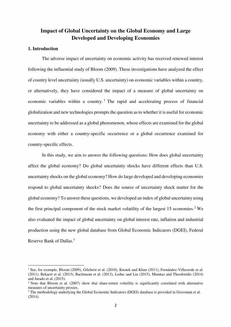
Impact of Global Uncertainty on the Global Economy and Large

Developed and Developing Economies

July 2017

Wensheng Kanga, Ronald A. Rattibce, Joaquin Vespignanide

aKent State University, Department of Economics, U.S. bUniversity of Missouri, Department of Economics, U.S.

cWestern Sydney University, School of Business, Australia dUniversity of Tasmania, Tasmanian School of Business and Economics, Australia

eCentre for Applied Macroeconomics Analysis, Australian National University, Australia

Abstract

Global uncertainty shocks are associated with a sharp decline in global inflation, growth and interest rate. From 1981 to 2014, global financial uncertainty forecasts 18.26% and 14.95% of the variation in global growth and global inflation, respectively. Global uncertainty shocks exhibit more protracted, statistically significant and substantial effects on the global growth, inflation and interest rate than U.S. uncertainty shocks. U.S. uncertainty lags global uncertainty by one month. When controlling for domestic uncertainty, the decline in output following a rise in global uncertainty is statistically significant in each country, with the exception of the decline for China. The effects for the U.S. and China are also relatively small. For most economies, a positive shock to global uncertainty has a depressing effect on prices and official interest rates – exceptions are Brazil, Mexico and Russia, which represent economies with large capital outflows during financial crises. Decomposition of global uncertainty shocks shows that global financial uncertainty shocks are more important than non-financial shocks. Keywords: Global, Uncertainty Shocks, Monetary Policy, FAVAR

JEL Codes: D80, E44, E66, F62, G10

Corresponding author: Joaquin Vespignani; University of Tasmania, Tasmanian School of Business and

Economics, Australia; Tel. No: +61 3 62262825; E-mail address: Joaquin.Vespignani@utas.edu.au

*We thank Baker Scott, Nicholas Bloom, Efrem Castelnuovo, Mardi Dungey, Enrique Martinez-Garcia and

Francesco Ravazzolo as well as our discussant James Hansen for useful comments of earlier versions. We also

thank members of Melbourne Institute, Centre for Applied Macro and Petroleum economics, Norges Bank and

BI Norwegian Business School and seminar participants at CAMP-Melbourne Institute Applied

Macroeconometrics Workshop (2015).

2

Impact of Global Uncertainty on the Global Economy and Large

Developed and Developing Economies

1. Introduction

The adverse impact of uncertainty on economic activity has received renewed interest

following the influential study of Bloom (2009). These investigations have analyzed the effect

of country level uncertainty (usually U.S. uncertainty) on economic variables within a country,

or alternatively, they have considered the impact of a measure of global uncertainty on

economic variables within a country. 1 The rapid and accelerating process of financial

globalization and new technologies prompts the question as to whether it is useful for economic

uncertainty to be addressed as a global phenomenon, whose effects are examined for the global

economy with either a country-specific occurrence or a global occurrence examined for

country-specific effects.

In this study, we aim to answer the following questions: How does global uncertainty

affect the global economy? Do global uncertainty shocks have different effects than U.S.

uncertainty shocks on the global economy? How do large developed and developing economies

respond to global uncertainty shocks? Does the source of uncertainty shock matter for the

global economy? To answer these questions, we developed an index of global uncertainty using

the first principal component of the stock market volatility of the largest 15 economies.2 We

also evaluated the impact of global uncertainty on global interest rate, inflation and industrial

production using the new global database from Global Economic Indicators (DGEI), Federal

Reserve Bank of Dallas.3

1 See, for example, Bloom (2009), Gilchrist et al. (2010), Knotek and Khan (2011), Fernández-Villaverde et al. (2011), Bekaert et al. (2013), Bachmann et al. (2013), Leduc and Liu (2015), Mumtaz and Theodoridis (2014) and Jurado et al. (2015). 2 Note that Bloom et al. (2007) show that share-return volatility is significantly correlated with alternative measures of uncertainty proxies. 3 The methodology underlying the Global Economic Indicators (DGEI) database is provided in Grossman et al. (2014).

3

The empirical literature on economic uncertainty has generally focused on the volatility

of stock market returns and/or firm profitability as providing a measure of uncertain

environments within which decisions are made.4 High uncertainty causes firms to postpone

investment and hiring and consumers to delay important purchases with unfavorable

consequences for economic growth. In a major paper, Bloom (2009) emphasizes the negative

impact of uncertainty on employment and output for the U.S. after World War II. In his work,

Bloom develops an uncertainty index based on firm stock return and/or firm profit growth.

An alternative measure of uncertainty based on spreads between low and high rated

corporate bonds are discussed by a number of authors, including contributions by Favero

(2009), Arellano et al. (2010) and Gilchrist et al. (2010). Bredin and Fountas (2009) utilize a

general bivariate GARCH-M model to generate the macroeconomic uncertainty associated

with output growth and inflation in EU countries. More recently, Jurado et al. (2015) argue that

stock market volatility may not be closely linked to “true” economic uncertainty, and they

propose new time series measures of macroeconomic uncertainty. These time series indicators

are built with U.S. macroeconomic data and are identified as the unforecastable component of

the macroeconomic series. Rossi and Sekhposyan (2015) develop a more general approach to

describe macroeconomic uncertainty. Their macroeconomic index is based on assessing the

likelihood of the realized forecast error of macroeconomic variables. Forecasts that are more

difficult to realize correspond to greater uncertainty in the macroeconomic environment.

Charemza et al. (2015) suggest a new measure of inflation forecast uncertainty that accounts

for possible inter-country dependence.

Berger and Herz (2014) measure global uncertainty as the conditional variances of

global factors in inflation and output growth in a bivariate dynamic factor model with GARCH

4 An important thread in the literature is that uncertainty faced by the individual firm is embodied in its own stock price volatility, as discussed in Leahy and Whited (1996), Bloom (2009), Bloom et al. (2007) and Baum et al. (2010), among others.

4

errors for nine industrialized countries: Canada, France, Germany, Italy, Japan, Netherlands,

Spain, United Kingdom and the United States. Delrio (2016) assumes that the spread between

each country’s interbank rate and the federal funds rate is a measure of relative riskiness. This

variable is then interacted with global uncertainty given by the realized volatility of daily MSCI

World Index returns over calendar quarters. Hirata et al. (2012) find that global house prices

are synchronized and that global uncertainty shocks seem to be important in explaining

fluctuations in global house prices. As in Bloom (2009), uncertainty is given by the volatility

of daily equity prices of the G-7. Ozturk and Sheng (2016) construct a monthly measure of

global uncertainty as the PPP-weighted average of the country-specific uncertainties for a

dataset of forecast data for 46 advanced and emerging market economies.

Leduc and Liu (2015) examine the effects of uncertainty – which are measured by

Michigan Survey results on the fraction of respondents reporting that an “uncertain future”

makes it a bad time to buy cars or durable goods over the next 12 months – on the U.S.

unemployment rate. Mumtaz and Theodoridis (2014) estimate the impact of U.S. GDP growth

volatility shocks on the UK in a structural VAR model with time-varying volatility.

In this study, we build on the methodology of Bloom (2009) to construct a global

uncertainty index using the first principal component of stock market volatility of 15 major

developed and developing economies. It provides a forward-looking indicator that is implicitly

weighted in accordance with the impact of different sources of uncertainty across major

countries in the world on equity value. Our measure of global uncertainty captures important

political, war, financial and economic events over the period 1981 to 2014 and shows high

correlations with alternative measures based on the methodology of Jurado et al. (2015) and

Ozturk and Sheng (2016).

The results show that global uncertainty shocks are less frequent than those observed

in data on the U.S. economy. The global uncertainty shocks are associated with a sharp decline

5

in global interest rate, inflation and industrial production. The maximum decline of global

inflation and industrial production occurs six months after a global uncertainty shock, while

the maximum decline in global interest rate occurs 16 months after a global uncertainty shock.

Our decomposition of global uncertainty shocks shows that global financial uncertainty

shocks are more important than non-financial shocks. From 1981 to 2014, global financial

uncertainty forecasts 18.26% and 14.95% of the variation in global growth and inflation,

respectively. In contrast, the non-financial uncertainty forecasts only 7.75% and 2.15% of the

variation in global growth and inflation, respectively. The effects of U.S. uncertainty on global

output, inflation and official interest rate are smaller and less statistically significant than the

effects of global uncertainty. Measures of U.S. uncertainty and global uncertainty are not

substitutable, and global uncertainty leads U.S. uncertainty by one month. Output declines in

each country with a rise in global uncertainty even controlling for domestic uncertainty, with

relatively small effects for the outputs of China and U.S. inflation and the official interest

decline with positive shocks to global uncertainty; exceptions include Brazil, Mexico and

Russia.

This paper proceeds as follows. An index of global uncertainty is constructed in Section

2. The effect of global uncertainty on the global economy is modeled in Section 3. In Section

4, preliminary results are examined with a FAVAR model. Section 5 compares the differences

between the U.S. and global uncertainty shocks. Section 6 examines the effects of global

uncertainty decomposed into financial and non-financial origins. The effect of global

uncertainty on individual major economies when controlling for local uncertainty is evaluated

in section 7. Section 8 provides robustness analysis, and Section 9 concludes.

2. An index of global uncertainty

2.1. Methodology

6

Empirical literature on economic uncertainty has utilized the variability of stock market

returns and firm profitability to provide a measure of uncertainty that can influence economic

and financial variables. In this study, we build upon this methodology by constructing a global

uncertainty index given by the first principal component of stock market volatility of the largest

15 economies. 5 It provides a forward-looking indicator that is implicitly weighted in

accordance with the impact of different sources of uncertainty across major countries in the

world on equity value.

Let 𝑅𝑐,𝑡 be the difference of the natural log of the stock market index of country 𝑐: 𝑅𝑐,𝑡 = ln 𝑆𝑐𝑡𝑆𝑐𝑡−1, (1)

where 𝑠𝑐𝑡 denotes the average monthly stock price for a given country 𝑐 at time 𝑡, with 𝑡 =1,2… , 𝑇. Let 𝑉𝑐𝑡 = (𝑅𝑐,𝑡 − �̅�𝑐,𝑡)2, (2)

where 𝑉𝑐𝑡 is the stock market volatility of country 𝑐 at time 𝑡, �̅�𝑐,𝑡 is the sample average of 𝑅𝑐,𝑡. The stock market volatility index is then estimated for the largest 15 economies in 2013

according to the gross domestic product (based on purchase power parity). The countries

include Australia, Brazil, Canada, China, Germany, France, India, Italy, Japan, Mexico, Russia,

South Korea, South Africa, the United Kingdom (U.K) and the United Sates (U.S).6

Given a data matrix with 𝑉𝑐𝑡 for the 15 largest economies and 𝑛 samples, we first

center on the means of 𝑉𝑐𝑡. The first principal component for the global uncertainty index (𝐺𝑈𝑡) is given by the linear combination of all 15 volatility

indices 𝑉𝐴𝑢𝑠𝑡𝑟𝑎𝑙𝑖𝑎,𝑡, 𝑉𝐵𝑟𝑎𝑧𝑖𝑙,𝑡,…., 𝑉𝑈𝑆,𝑡,. Formally, 𝐺𝑈𝑡 = 𝑎1𝑉𝐴𝑢𝑠𝑡𝑟𝑎𝑙𝑖𝑎,𝑡 + 𝑎2𝑉𝐵𝑟𝑎𝑧𝑖𝑙,𝑡 + ⋯+ 𝑎15𝑉𝑈𝑆,𝑡. (3)

5 This first principal component accounts for around 40% of the data variation. 6 We attempt to estimate this index for G20 economies. However, data for Indonesia, Iran, Thailand Nigeria and Poland were not available for the full sample period. An alternative measure of global uncertainty including these countries for a shorter span is discussed in section 8.6.

7

𝐺𝑈𝑡 is calculated such that it accounts for the greatest possible variance in the data set. The

weights (𝑎𝑖) are the elements of an eigenvector with unit length and standardized by the

restriction: 𝑎12 + 𝑎22 + ⋯+ 𝑎152 = 1. Data definitions, sources and period availabilities are all

reported in Table A1.7

2.2. Global and the U.S. uncertainty indices

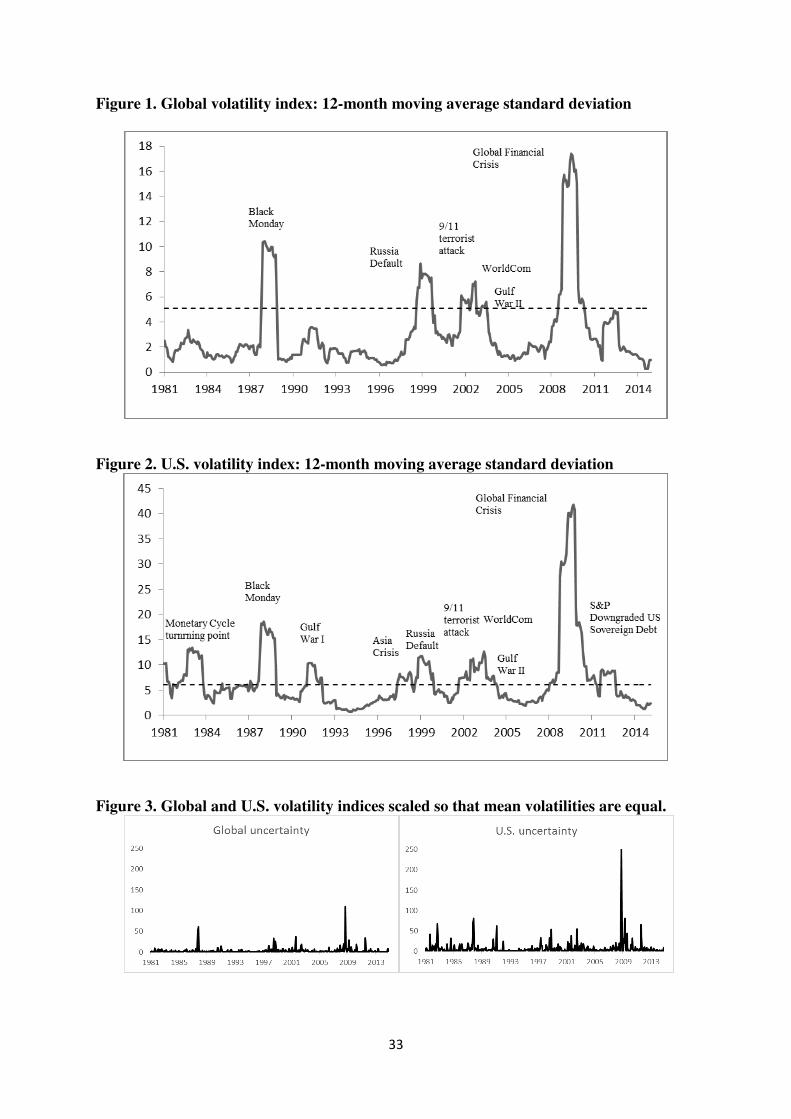
In Figures 1 and 2, we show the global uncertainty index developed in Equation (1) to

(3) and the U.S. uncertainty index.8 In each Figure, the black line shows the 12-month moving

average of the index, and the horizontal broken line shows 1.65 standard deviations. We follow

Bloom (2009) and Jurado et al. (2015) in defining uncertainty shocks as those events which

exceed 1.65 standard deviations. By comparing Figure 1 with Figure 2, several points can be

made.

The statistically significant global uncertainty shocks shown in Figure 1 are associated

with Black Monday (October and November 1987), the Russian Default (September 1998), the

9/11 terrorist attack (September 2001), WorldCom (July 2002), the Gulf War II (February

2003) and the Global Financial Crisis (GFC) between 2007-2008. The non-economic

statistically significant global uncertainty shocks, the 9/11 attack and Gulf War II are smaller

than the economic statistically significant global uncertainty shocks in Figure 1. The

statistically significant global uncertainty shocks shown in Figure 1 are also statistically

significant U.S. uncertainty shocks in Figure 2.

On Monday, October 19, 1987, stock markets around the world collapsed. The fall

started in Hong Kong and spread west to Europe; in the United States, the Dow Jones Industrial

7 Data from the stock market are not available for all countries from 1981. The index is constructed with data on the countries for which data are available. A shortcoming of this approach is that for the earlier period, missing data are more apparent for developing countries. Nevertheless, we argue that this is not necessarily a problem, given that in the first part of the sample (1980-1995), the relative weight of developed economies in the global economy is more important than in the more recent period (following China’s unprecedented growth starting in mid-1990s). The availability of stock market data for each country is reported in Table A1 in Appendix A. 8 The last is just the stock market volatility index constructed with only the data for the U.S. stock market.

8

Average fell by 22.6%. Globally, stock market losses persisted, with markets in Hong Kong,

the United Kingdom and the United States down by 45.5%, 26.5% and 22.7%, respectively, at

the end of October 1987. Despite October 19, 1987 being the biggest daily percentage decline

in the history of the Dow Jones Index, no major (news) event has been associated with the

stock market crash. Both the monthly U.S. stock market volatility and the monthly global stock

market volatility were high during October 1987, but they were both even higher during

November 1987.

On August 17, 1998, the Russian Central Bank devalued the rubble, and the Russian

government defaulted on its debt. The background of these developments included high

inflation (Russian inflation was over 80% during 1998) and the loss of foreign exchange

reserves associated with decreased revenues from the export of crude oil and other commodities

attendant on falling prices and weak demand in the aftermath of the Asian Financial Crisis in

late 1997. The Russian devaluation and default caused the Long Term Capital Management

hedge fund to default on financial contracts worth billions of dollars, leading the Federal

Reserve Bank of New York to orchestrate a rescue effort to avert a major financial collapse.

During this episode, the monthly U.S. stock market volatility was highest during August 1998,

as was the global stock market volatility.

The 9/11 terrorist attack in September 2001 is associated with spikes in volatility in

both the monthly U.S. stock market volatility and the monthly global stock market volatility.

In July 2002, large overstated revenues were uncovered in an accounting scandal at WorldCom,

and the monthly U.S. and global stock market volatility spiked. A series of accounting scandals

had started at Enron in December 2001 and at a number of large companies including

WorldCom throughout 2002.

The Gulf War II started on March 19 and continued to May 1 in 2003. Monthly U.S.

and global stock market volatilities increased sharply in February 2003 in anticipation of the

9

U.S. invasion of Iraq. Over the next three months, global stock market volatility fell to

somewhat less than half the value achieved in February 2003 before rising to about 73% of the

February 2003 level in June 2003. In contrast, the monthly U.S. stock market volatility fell to

a very low value in March 2003 and achieved values from April to June 2003 of between 73%

and 89% of the value in February 2003. The implications of this pattern of volatility is that, in

the moving average plots of data in Figures 1 and 2 from September 2001 to June 2003, the

monthly U.S. stock market volatility peaks in June 2003 (in the aftermath of the Gulf War II),

whereas the monthly global stock market volatility peaks in September 2002 (during the

accounting scandals).

The GFC includes several events described in detail in Table A3 (Appendix A). The

crisis is associated with the subprime mortgage crisis, including the consequent bankruptcy of

Lehman Brothers in September 2008 and the bailout of several financial institutions including

Northern Rock in UK (February 2008) as well as Fannie Mae and Freddie Mac (July 2008) and

American International Group (September 2008) in the U.S.

Standard & Poor downgraded U.S. sovereign debt from AAA to AA+ on August 5,

2011. Both U.S. stock market volatility and global stock market volatility spiked in August

2011. The 12-month moving average for volatility peaked in May 2012 in global stock markets

and in September 2011 for the U.S. stock market. This difference in timing is apparent when

comparing Figures 1 and 2.

The uncertainty associated with the Monetary Cycle turning point (October 1982), the

Gulf War I (October 1990) and the Asian Crisis (November 1997) are statistically significant

in the U.S. data depicted in Figure 2 but not in the global data represented in Figure 1. The

market volatility during the Monetary Cycle turning point is identified with uncertainty over

the effectiveness of policy during the Reagan administration at dealing with inflation and

recession. The global uncertainty shock associated with the Monetary Cycle turning point is

10

not statistically significant in Figure 1. Both the monthly volatility and the 12-month moving

average volatility for the global stock markets peak in September 1982 and fall in the following

months. The monthly volatility in the U.S. data also peaks in September 1982 and then falls in

following months. The 12-month moving average volatility for the U.S. stock market has high

values over the whole period September 1982 to September 1983. A peak in September 1982

is exceeded slightly in November 1982 and in January 1983. Overall, the Monetary Cycle

turning point is a much more important uncertainty event in the U.S. data than in the global

data.

2.3. Relative importance of high uncertainty events in U.S. and global data

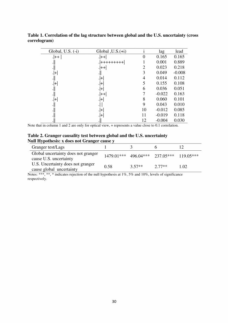
Table 1 reports the correlation of the lag structure between global uncertainty and the

measure of U.S. uncertainty. The contemporaneous correlation between global and U.S.

uncertainties is 0.16. The other correlations in Table 1 are less than 0.16 with two exceptions.

The exceptions are that the lagged correlations of U.S. uncertainty and global uncertainty are

0.89 and 0.208 for lags of 1 and 2 months, respectively. The implication for the one-month-lag

correlation is that if the global uncertainty is high is June, then the U.S. uncertainty is likely to

be high in July.

Table 2 reports the Granger causality test between global uncertainty and U.S.

uncertainty. The null hypothesis is that global uncertainty does not cause U.S. uncertainty, and

the Granger results show that the null hypothesis can be rejected at 1% level of confidence with

lags of 1, 3, 6 and 12 months. The null hypothesis that U.S. uncertainty does not cause global

uncertainty cannot be rejected with lags of 1 and 12 months. The correlation and Granger

causality results support the idea that the measures of U.S. uncertainty and global uncertainty

are not interchangeable and that, for the most part, U.S. uncertainty is not driving the measure

of global uncertainty.

11

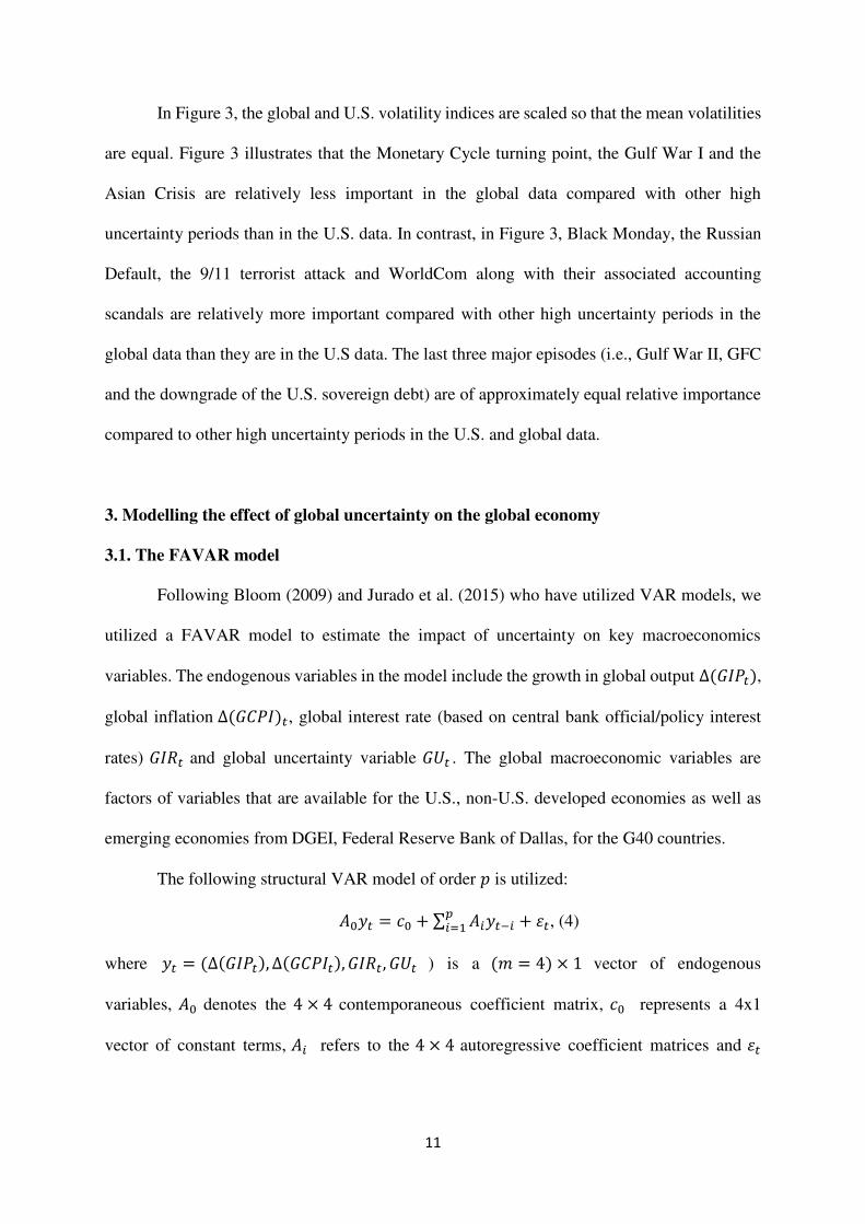
In Figure 3, the global and U.S. volatility indices are scaled so that the mean volatilities

are equal. Figure 3 illustrates that the Monetary Cycle turning point, the Gulf War I and the

Asian Crisis are relatively less important in the global data compared with other high

uncertainty periods than in the U.S. data. In contrast, in Figure 3, Black Monday, the Russian

Default, the 9/11 terrorist attack and WorldCom along with their associated accounting

scandals are relatively more important compared with other high uncertainty periods in the

global data than they are in the U.S data. The last three major episodes (i.e., Gulf War II, GFC

and the downgrade of the U.S. sovereign debt) are of approximately equal relative importance

compared to other high uncertainty periods in the U.S. and global data.

3. Modelling the effect of global uncertainty on the global economy

3.1. The FAVAR model

Following Bloom (2009) and Jurado et al. (2015) who have utilized VAR models, we

utilized a FAVAR model to estimate the impact of uncertainty on key macroeconomics

variables. The endogenous variables in the model include the growth in global output ∆(𝐺𝐼𝑃𝑡),

global inflation ∆(𝐺𝐶𝑃𝐼)𝑡, global interest rate (based on central bank official/policy interest

rates) 𝐺𝐼𝑅𝑡 and global uncertainty variable 𝐺𝑈𝑡 . The global macroeconomic variables are

factors of variables that are available for the U.S., non-U.S. developed economies as well as

emerging economies from DGEI, Federal Reserve Bank of Dallas, for the G40 countries.

The following structural VAR model of order 𝑝 is utilized: 𝐴0𝑦𝑡 = 𝑐0 + ∑ 𝐴𝑖𝑦𝑡−𝑖𝑝𝑖=1 + 𝜀𝑡, (4)

where 𝑦𝑡 = (∆(𝐺𝐼𝑃𝑡), ∆(𝐺𝐶𝑃𝐼𝑡), 𝐺𝐼𝑅𝑡, 𝐺𝑈𝑡 ) is a (𝑚 = 4) × 1 vector of endogenous

variables, 𝐴0 denotes the 4 × 4 contemporaneous coefficient matrix, 𝑐0 represents a 4x1

vector of constant terms, 𝐴𝑖 refers to the 4 × 4 autoregressive coefficient matrices and 𝜀𝑡

12

stands for a 4 × 1 vector of structural disturbances.9 To construct the structural VAR model

representation, the reduced-form VAR model is consistently estimated using the least-squares

method and is obtained by multiplying both sides of Equation (4) by 𝐴0−1. The reduced-form

error term is 𝑒𝑡 = 𝐴0−1𝜀𝑡 and is assumed to be Gaussian distributed.

The identifying restrictions on 𝐴0−1 is a lower-triangle coefficient matrix in the

structural VAR model. This setup follows Christiano et al. (2005), Bekaert et al. (2014) and

Jurado et al. (2015) in placing the output variable first, followed by global consumer price

index (CPI), global interest rate and global uncertainty.10 The ordering of the variables assumes

that the macroeconomic aggregates of output and CPI do not respond contemporaneously to

shocks to the monetary policy of interest rate. The information of the monetary authority within

a month 𝑡 consists of current and lagged values of the macroeconomic aggregates and past

values of the uncertainty. The uncertainty variable ordered last captures the fact that the

uncertainty is a stock-market-based variable and responds instantly to monetary policy shocks.

The structural shocks to the dynamic responses of an endogenous variable are then identified

using a Cholesky decomposition.

3.2. Data and global macroeconomic variables

The data for both the global uncertainty index and the VAR models are monthly and

extend from January 1981 to December 2014. Before 1981, data are not available for most

variables from many developing countries. Data descriptions, sources and period availabilities

are presented in Table A2.

The global factors 𝐺𝐼𝑅𝑡 , 𝐺𝐶𝑃𝐼𝑡 and 𝐺𝐼𝑃𝑡 are estimated using data on emerging

economies, advanced economies (excluding the U.S.) and the U.S. The data on interest rate,

9 We follow Bloom (2009) and Jurado et al. (2015) in setting p=12, which allows for a potentially long-delay of effects of uncertainty shocks on the economy and for a sufficient number of lags to remove serial correlation. 10 We omitted the variables stock prices, wages, working hours and employment because these variables are not available at the global level.

13

CPI and industrial production are taken from DGEI, Federal Reserve Bank of Dallas, for the

G40 countries. In DGEI, weights (based on shares of world GDP [PPP]) are applied to the

official/policy interest rates (determined by central banks) in levels and are applied to the

indexes for industrial production and headline price indexes in growth rates to construct indices

for emerging economies and advanced economies (excluding the U.S). In 2014, on a GDP PPP

basis, the G40 economies account for 83% of the global GDP. Also, within the G40, the U.S.,

19 advanced economies (excluding the U.S.) and 20 emerging economies account for 18%,

25%, and 40%, respectively, of the global GDP. Combined, the 20 largest emerging economies

on a PPP basis are now nearly as large as the 20 largest developed economies. 𝐺𝐼𝑅𝑡, 𝐺𝐶𝑃𝐼𝑡 and 𝐺𝐼𝑃𝑡 are the leading principal components: 𝐺𝐼𝑅𝑡 = [𝐼𝑅𝑡𝐴𝑑, 𝐼𝑅𝑡𝑈𝑆, 𝐼𝑅𝑡𝐸𝑚], (5) 𝐺𝐶𝑃𝐼𝑡 = [𝐶𝑃𝐼𝑡𝐴𝑑, 𝐶𝑃𝐼𝑡𝑈𝑆, 𝐶𝑃𝐼𝑡𝐸𝑚], (6) 𝐺𝐼𝑃𝑡 = [𝐼𝑃𝑡𝐴𝑑, 𝐼𝑃𝑡𝑈𝑆, 𝐼𝑃𝑡𝐸𝑚], (7)

where the superscripts US, Ad and Em represent the United States, advanced economies

(excluding the U.S) and emerging economies.11

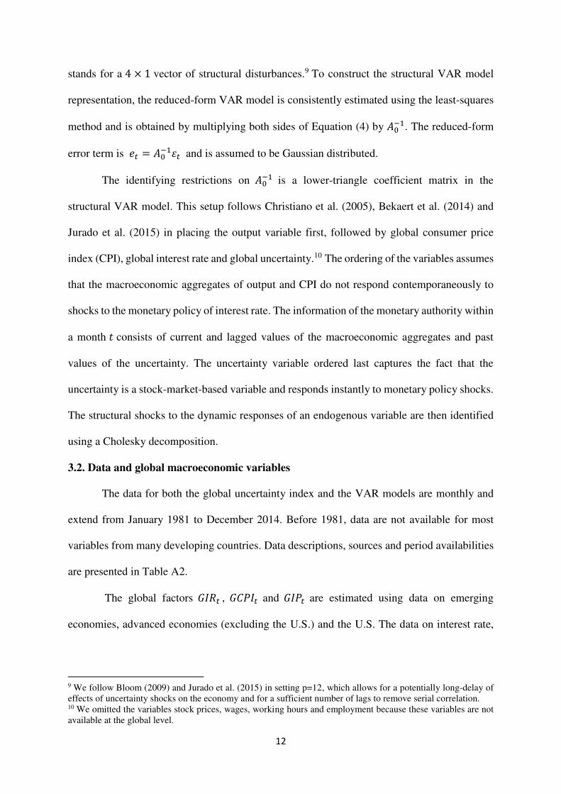
4. The FAVAR model results

The reduced-form VAR model of Equation (4) is consistently estimated by the ordinary

least squares (OLS) method. We utilize the resulting estimates to construct the structural VAR

representation of the model. The dynamic effect is examined by the impulse responses of global

output growth, inflation and interest rate to the structural global uncertainty shock. We present

the responses to one-time global uncertainty shocks as well as to the historical episodes of the

uncertainty shocks.

11 We deal with missing data in early observations for some series by building the factors with series available at this time to maximise the number of time series observations.

14

4.1. The effects of global uncertainty shocks on the economy

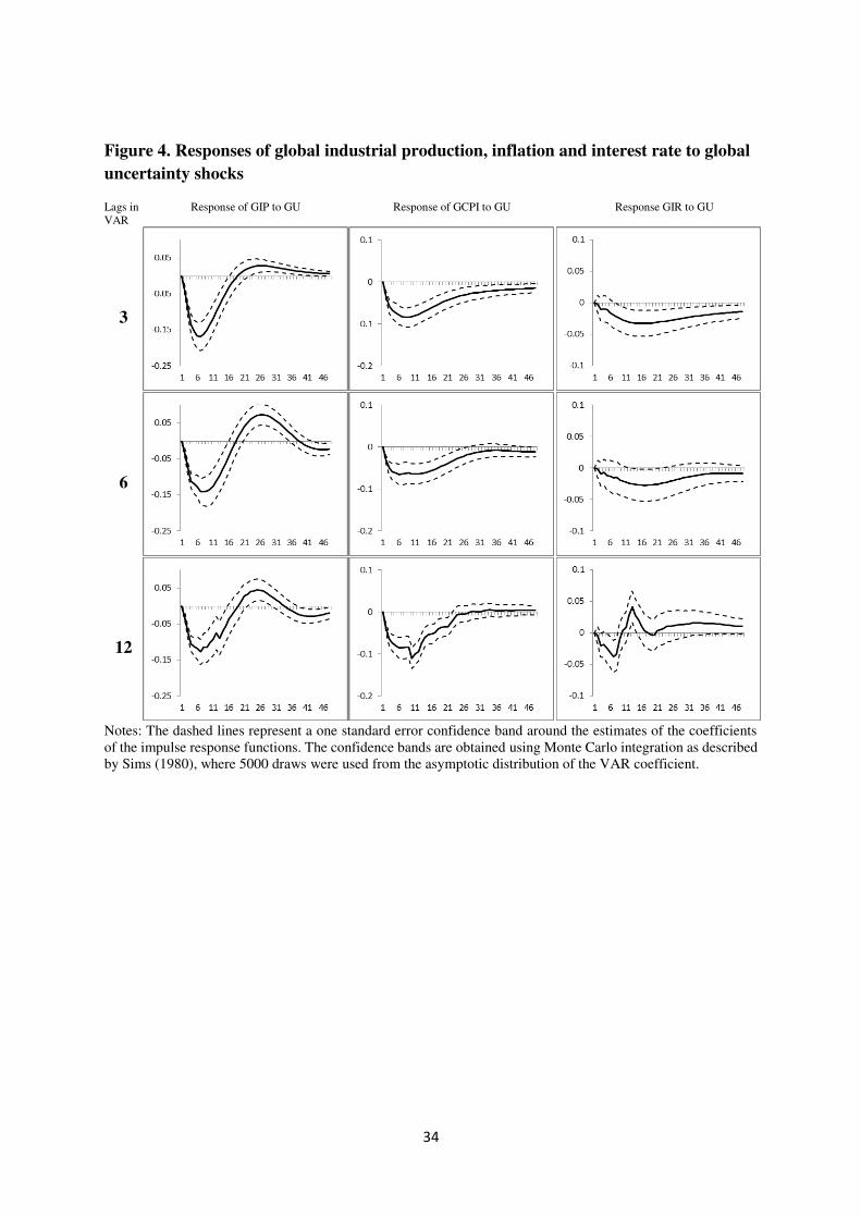
Figure 4 shows the impact of one standard deviation of the global uncertainty shocks

on global industrial production growth, global CPI inflation and global interest rate for the

FAVAR estimation. The dashed lines represent a one-standard-error confidence band around

the estimates of the coefficients of the impulse response functions. We utilize the impulse

response functions in Figure 4 to assess the timing and magnitude of the responses to a one-

time global uncertainty shock in the economy.

On the left hand side of Figure 4, the estimated lags in the VAR system are indicated.

The FAVAR model is estimated with 3, 6 and 12 lags. The second, third and fourth columns

in Figure 4 show responses of global interest rate, CPI inflation and industrial production

growth to global uncertainty shocks. The results are summarized as follows:

Global uncertainty shocks are associated with a quick and sharp decline in global

industrial production growth, which is greatest after 4 to 8 months depending on the

specification.

Global uncertainty shocks are associated with a quick and sharp decline in global CPI,

reaching the greatest point of decline after 6 months. However, when 12 lags are used

in the VAR system, the greatest point of decline occurs after 10 months.

Global uncertainty shocks are associated with a decline in global interest rate; when 3-

and 6-month lags are used in the VAR systems, the greatest decline in the global interest

rate is observed after 16 months.12

12 When the models are specified with 12 lags, the greatest response occurs after 6 months, with a quick return to positive values after 12 months. This pattern is only observed for FAVAR model, and for the FABVAR model, Wishart type of priors in models with a 12-month lag. Even with a 12-month lag structure, the FABVAR model with Minnesota and Sims-Zha priors gives results that are similar to those obtained in the FAVAR and FABVAR models with 3-month and 6-month lags.

15

5. Does the global economy respond differently to global uncertainty shocks compared to

U.S. uncertainty shocks?

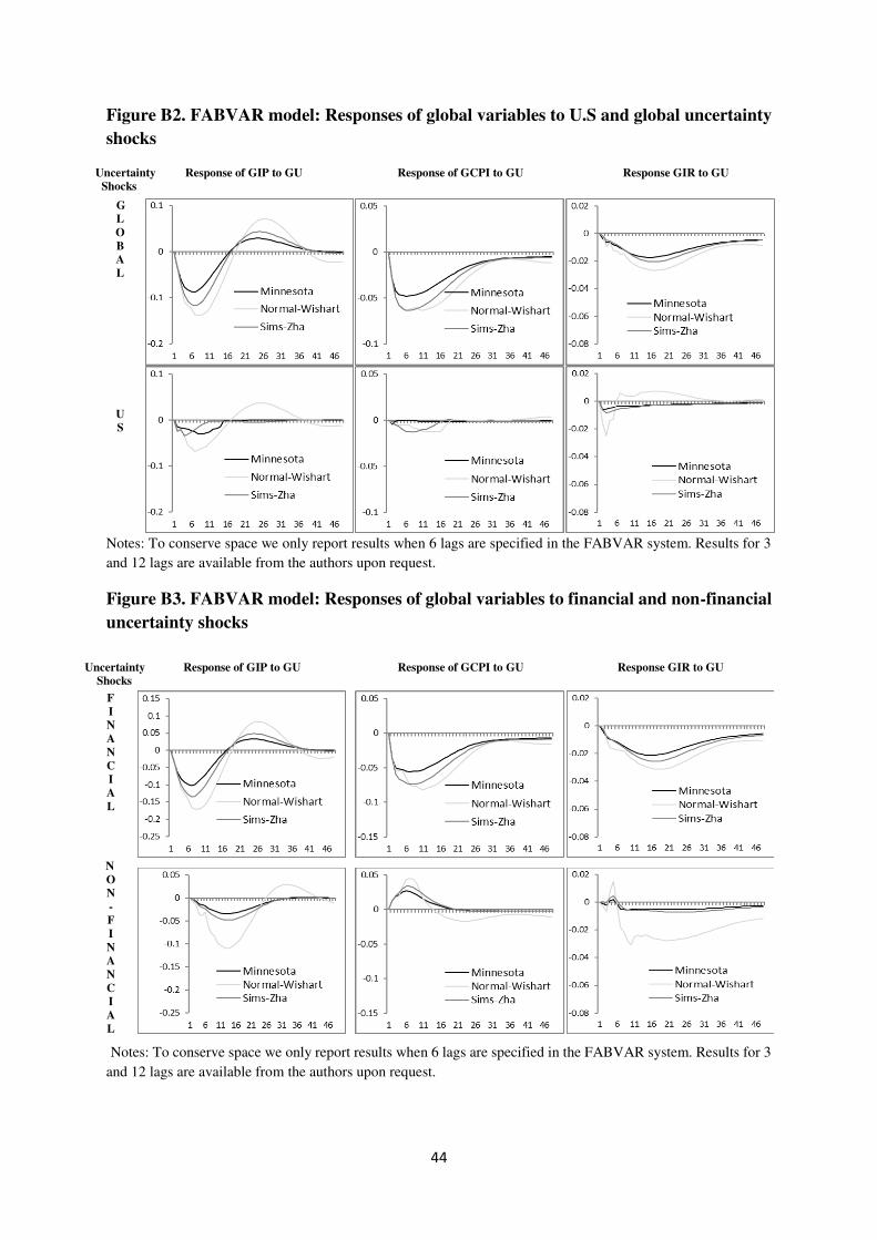
Given that the U.S. is the world’s largest financial centre, we disaggregate the effects

of U.S. uncertainty (𝑈𝑆𝑈𝑡) and global uncertainty. U.S. uncertainty is estimated as a volatility

index of the U.S. stock market. The new vector of endogenous variables is a (𝑚 = 5) × 1

vector of endogenous variables: 𝑦𝑡 = (∆(𝐺𝐼𝑃𝑡), ∆(𝐺𝐶𝑃𝐼𝑡), 𝐺𝐼𝑅𝑡 , 𝑈𝑆𝑈𝑡, 𝐺𝑈𝑡). 𝐴0 denotes the 5 × 5 contemporaneous coefficient matrix. More precisely, the Cholesky lower triangle

contemporaneous matrix is estimated by postulating the following 𝐴0𝑦𝑡 matrix form:

[ 1 0 0 0 0𝑎11 1 0 0 0𝑎21 𝑎22 1 0 0𝑎31 𝑎32 𝑎33 1 0𝑎41 𝑎42 𝑎43 0 1]

[ ∆(𝐺𝐼𝑃𝑡)∆(𝐺𝐶𝑃𝐼𝑡)𝐺𝐼𝑅𝑡𝑈𝑆𝑈𝑡𝐺𝑈𝑡 ]

, (8)

where 𝑈𝑆𝑈𝑡 represents the U.S uncertainty shock derived from the volatility of the U.S. stock

market. Note that coefficient 𝑎44 is set to be zero; this implies that we do not have a preference

for ordering either the U.S. or global uncertainty first in the Cholesky decomposition.13

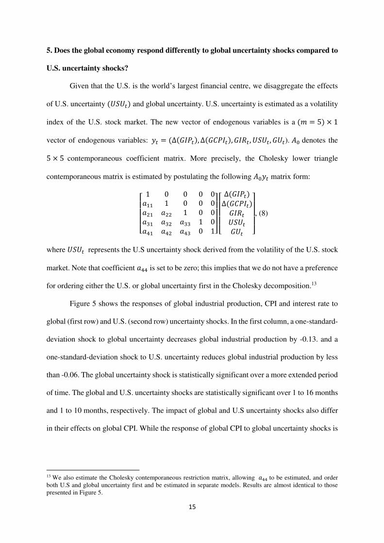
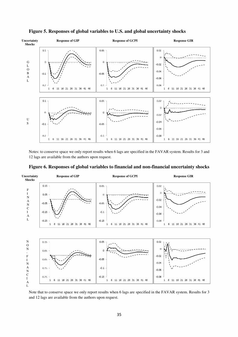
Figure 5 shows the responses of global industrial production, CPI and interest rate to

global (first row) and U.S. (second row) uncertainty shocks. In the first column, a one-standard-

deviation shock to global uncertainty decreases global industrial production by -0.13. and a

one-standard-deviation shock to U.S. uncertainty reduces global industrial production by less

than -0.06. The global uncertainty shock is statistically significant over a more extended period

of time. The global and U.S. uncertainty shocks are statistically significant over 1 to 16 months

and 1 to 10 months, respectively. The impact of global and U.S uncertainty shocks also differ

in their effects on global CPI. While the response of global CPI to global uncertainty shocks is

13 We also estimate the Cholesky contemporaneous restriction matrix, allowing 𝑎44 to be estimated, and order both U.S and global uncertainty first and be estimated in separate models. Results are almost identical to those presented in Figure 5.

16

statistically significant and reaches a minimum of -0.08, the impact of U.S. uncertainty shocks

on global CPI is much smaller and is not statistically significant at conventional levels.

Finally, the global interest rate is negatively affected by a positive global uncertainty

shock, but the effect is only marginally statistically significant. The response of global interest

rate to U.S uncertainty shocks is much smaller and is not statistically significant.

6. Does the source of uncertainty shocks matter for the global economy?

The central result in Section 4.2 is that the global uncertainty shocks have very different

effects on the economy at different points in time. In this section, we show that global

uncertainty shocks have different sources. We analyse the impact of global uncertainty shocks

looking at their sources. In particular, we decompose global uncertainty shocks into global

financial and non-financial shocks, where the shocks considered are those shocks that exceed

1.65 standard deviations in terms of monthly observations.

6.1. Financial vs. non-financial uncertainty shock

In this subsection, we distinguish between financial and non-financial shocks and

estimate the impact effects of both shocks on the global economy. Shocks originating in

economic or financial disruption may have been amenable to better economic policy design,

whereas those due to war or terrorism are not (although political policies might have an impact).

Examination of uncertainty shocks with an economic/financial source might lead to a better

understanding of how economic policy might be designed to both avoid and mitigate the effects

of future shocks.

Our definition of global financial shocks comprises the following events that exceeded

1.65 standard deviations: Black Monday, Russian Default, WorldCom and the GFC. The global

financial crisis includes the five main events described in Table A3 (Appendix A), including

the North Rock emergency funding in September 2007 and the nationalisation in February

17

2008, the bailout of Fannie Mae and Freddie Mac, the Lehman Brothers bankruptcy and the

bail out of American International Group (AIG) in the U.S in July 2008, September 2008 and

October 2008, respectively. The non-financial uncertainty shocks that exceed 1.65 standard

deviations include the Gulf War II and the 9/11 terrorist attack.

To disaggregate global uncertainty shocks, we modify the system of equations by

subtitling the unique variable 𝐺𝑈𝑡 into two different uncertainty shocks (i.e., 𝐷𝐹 ∗ 𝐺𝑈𝑡 and 𝐷𝑁𝐹 ∗ 𝐺𝑈𝑡), where the first variable the global financial uncertainty shock is constructed by

interacting the 𝐺𝑈𝑡 index with a dummy variable 𝐷𝐹𝑡 , which takes the value of 1 when a

financial shock occurs and 0 otherwise. Details of the period dummies can be found in

Appendix A, Table A4. 14 The second variable (the non-financial uncertainty shocks) is

constructed by interacting the 𝐺𝑈𝑡 index with a dummy variable 𝐷𝑁𝐹𝑡, which takes the value

of 1 when a non-financial shock occurs and 0 otherwise.15 The new vector of endogenous

variables is a (𝑚 = 5) × 1 vector, that is, 𝑦𝑡 = (∆(𝐺𝐼𝑃𝑡), ∆(𝐺𝐶𝑃𝐼𝑡), 𝐺𝐼𝑅𝑡, 𝐹𝐷𝐹𝑡 ∗𝐺𝑈𝑡𝑈𝑡, 𝐷𝑁𝐹𝑡 ∗ 𝐺𝑈𝑡). The Cholesky lower triangle contemporaneous matrix is estimated using

the following 𝐴0𝑦𝑡 matrix:

[ 1 0 0 0 0𝑎11 1 0 0 0𝑎21 𝑎22 1 0 0𝑎31 𝑎32 𝑎33 1 0𝑎41 𝑎42 𝑎43 0 1]

[ ∆(𝐺𝐼𝑃𝑡)∆(𝐺𝐶𝑃𝐼𝑡)𝐺𝐼𝑅𝑡𝐷𝐹𝑡 ∗ 𝐺𝑈𝑡𝐷𝑁𝐹𝑡 ∗ 𝐺𝑈𝑡]

(9)

We set 𝑎44 to be zero, since there is no good reason to impose an order on financial and non-

financial uncertainty. 16

14 The dummy variables only take the value of 1 when the identified shock exceeds 1.65 standard deviations following Bloom (2009). 15 We slightly innovate with respect of Bloom (2009), who uses only a single dummy variable that takes the value of 1 when the uncertainty shock occurs and 0 otherwise. The reason for doing that is because Bloom (2009)’s definition does not capture the magnitude of the shock. By interacting the 𝐺𝑈𝑡 and a dummy variable, the shocks now also capture the dimension of the shock. 16 Either eliminating the zero restriction on 𝑎44 and/or changing the order financial and non-financial uncertainty shocks do not alter the main results.

18

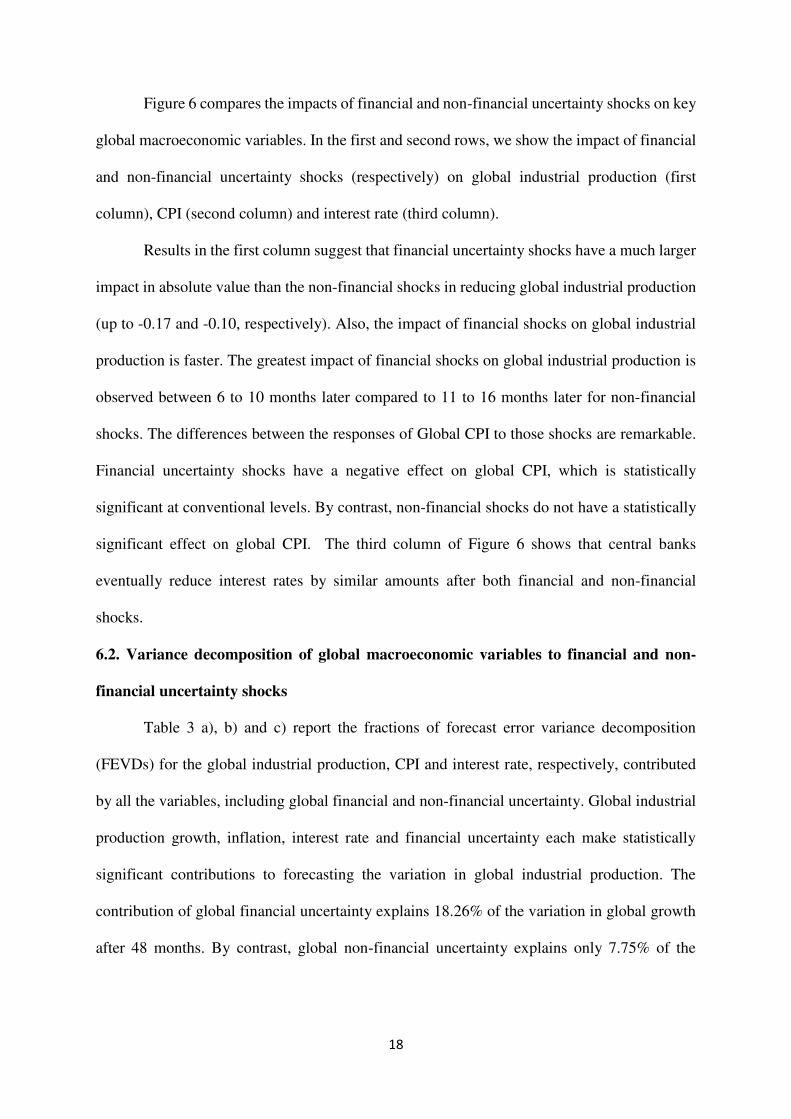
Figure 6 compares the impacts of financial and non-financial uncertainty shocks on key

global macroeconomic variables. In the first and second rows, we show the impact of financial

and non-financial uncertainty shocks (respectively) on global industrial production (first

column), CPI (second column) and interest rate (third column).

Results in the first column suggest that financial uncertainty shocks have a much larger

impact in absolute value than the non-financial shocks in reducing global industrial production

(up to -0.17 and -0.10, respectively). Also, the impact of financial shocks on global industrial

production is faster. The greatest impact of financial shocks on global industrial production is

observed between 6 to 10 months later compared to 11 to 16 months later for non-financial

shocks. The differences between the responses of Global CPI to those shocks are remarkable.

Financial uncertainty shocks have a negative effect on global CPI, which is statistically

significant at conventional levels. By contrast, non-financial shocks do not have a statistically

significant effect on global CPI. The third column of Figure 6 shows that central banks

eventually reduce interest rates by similar amounts after both financial and non-financial

shocks.

6.2. Variance decomposition of global macroeconomic variables to financial and non-

financial uncertainty shocks

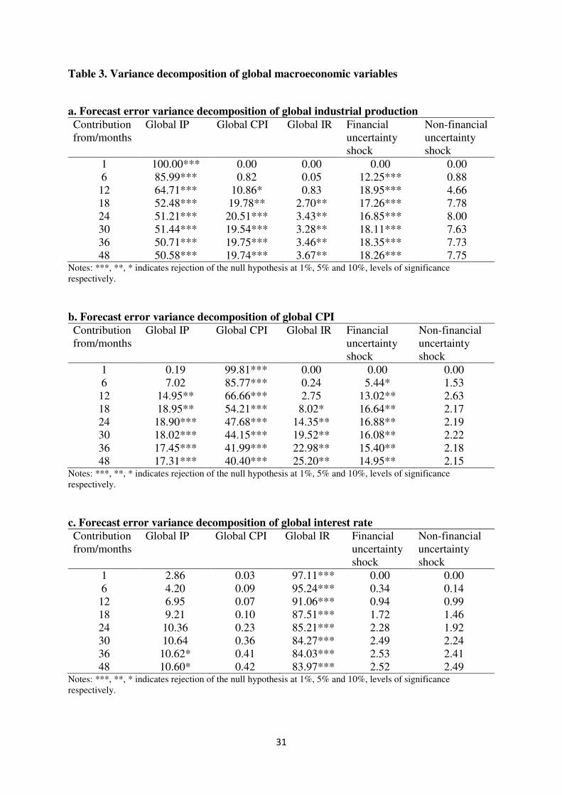
Table 3 a), b) and c) report the fractions of forecast error variance decomposition

(FEVDs) for the global industrial production, CPI and interest rate, respectively, contributed

by all the variables, including global financial and non-financial uncertainty. Global industrial

production growth, inflation, interest rate and financial uncertainty each make statistically

significant contributions to forecasting the variation in global industrial production. The

contribution of global financial uncertainty explains 18.26% of the variation in global growth

after 48 months. By contrast, global non-financial uncertainty explains only 7.75% of the

19

variation in global growth (that is not statistically significant) after 48 months. After 48 months,

global inflation and interest rate forecast 19.74% and 3.67% of variation in global growth.

Global industrial production growth, interest rate, and financial uncertainty each make

statistically significant contributions to forecasting the variation in global inflation, while

global non-financial uncertainty does not. The contribution of global financial uncertainty

explains 14.95% of the variation in global inflation after 48 months. In contrast to the effect on

global industrial production, the global interest rate explains a large fraction variation (25.20%)

in global inflation after 48 months. Only global growth explains a statistically significant

fraction (10.60% after 48 months) of the variation in global interest rate.

In summary, the forecast error variance decomposition results indicate that global

financial uncertainty explains statistically significant fractions of the variation in global growth

and global inflation over 48-month horizons, while global non-financial uncertainty does not.

At the 48-month horizon, global financial uncertainty accounts for 18.26% and 14.95% of the

variation in global growth and inflation, respectively.

7. Effect of global uncertainty in presence of local uncertainty for domestic economies

To determine whether the effect of global uncertainty on local macroeconomic

variables is robust to the inclusion of local uncertainty, we re-estimate the SVAR for the largest

developed and developing economies with both global and domestic uncertainty included as

variables. The models are estimated separately for each economy.

The model is described in Equation 10, where the first four variables in the SVAR

system are variables for a specific economy and the last variable is global uncertainty. The

endogenous variables in the model can be summarized as follows: 𝑦𝑡 = (∆(𝐷𝐼𝑃𝑡), ∆(𝐷𝐶𝑃𝐼𝑡), 𝐷𝐼𝑅𝑡 , 𝐷𝑈𝑡, 𝐺𝑈𝑡),

20

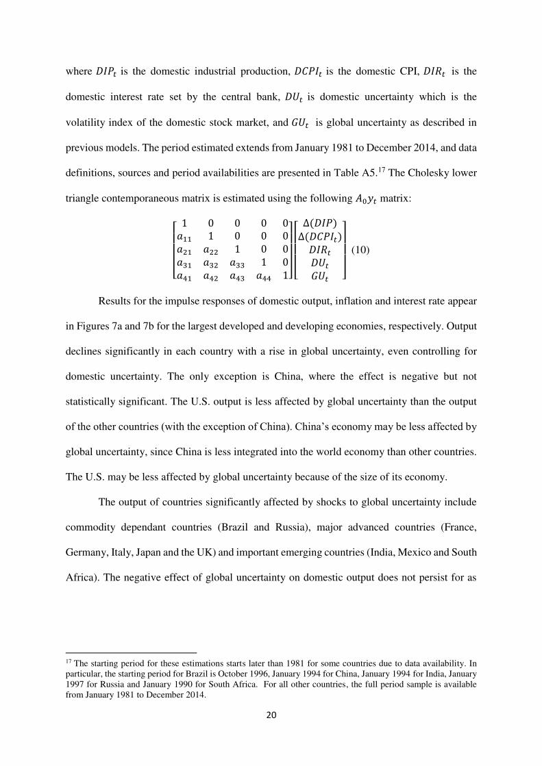
where 𝐷𝐼𝑃𝑡 is the domestic industrial production, 𝐷𝐶𝑃𝐼𝑡 is the domestic CPI, 𝐷𝐼𝑅𝑡 is the

domestic interest rate set by the central bank, 𝐷𝑈𝑡 is domestic uncertainty which is the

volatility index of the domestic stock market, and 𝐺𝑈𝑡 is global uncertainty as described in

previous models. The period estimated extends from January 1981 to December 2014, and data

definitions, sources and period availabilities are presented in Table A5.17 The Cholesky lower

triangle contemporaneous matrix is estimated using the following 𝐴0𝑦𝑡 matrix:

[ 1 0 0 0 0𝑎11 1 0 0 0𝑎21 𝑎22 1 0 0𝑎31 𝑎32 𝑎33 1 0𝑎41 𝑎42 𝑎43 𝑎44 1]

[ ∆(𝐷𝐼𝑃)∆(𝐷𝐶𝑃𝐼𝑡)𝐷𝐼𝑅𝑡𝐷𝑈𝑡𝐺𝑈𝑡 ]

(10)

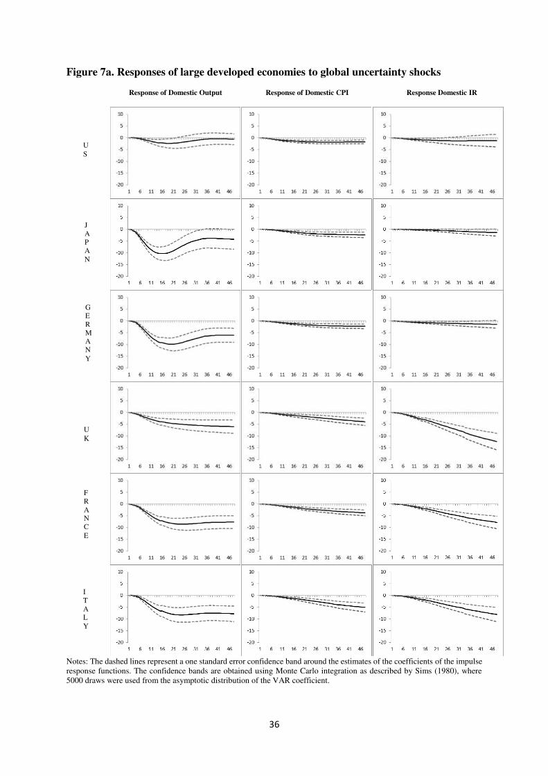
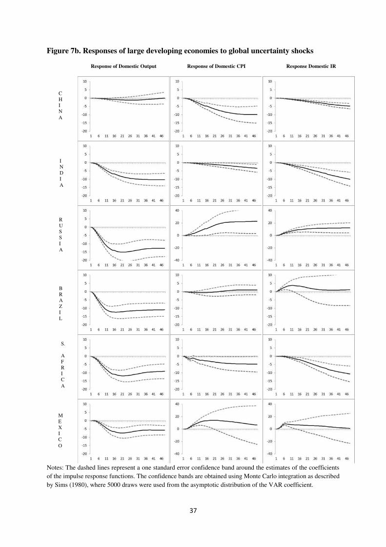
Results for the impulse responses of domestic output, inflation and interest rate appear

in Figures 7a and 7b for the largest developed and developing economies, respectively. Output

declines significantly in each country with a rise in global uncertainty, even controlling for

domestic uncertainty. The only exception is China, where the effect is negative but not

statistically significant. The U.S. output is less affected by global uncertainty than the output

of the other countries (with the exception of China). China’s economy may be less affected by

global uncertainty, since China is less integrated into the world economy than other countries.

The U.S. may be less affected by global uncertainty because of the size of its economy.

The output of countries significantly affected by shocks to global uncertainty include

commodity dependant countries (Brazil and Russia), major advanced countries (France,

Germany, Italy, Japan and the UK) and important emerging countries (India, Mexico and South

Africa). The negative effect of global uncertainty on domestic output does not persist for as

17 The starting period for these estimations starts later than 1981 for some countries due to data availability. In particular, the starting period for Brazil is October 1996, January 1994 for China, January 1994 for India, January 1997 for Russia and January 1990 for South Africa. For all other countries, the full period sample is available from January 1981 to December 2014.

21

long in Japan as for most other countries, possibly due to relatively high levels of economic

association with China’s economy.

The responses of inflation and the official interest to positive shocks to global

uncertainty are mostly negative and consistent with the result for the negative effect of shocks

to global uncertainty on output. For most economies, a positive shock to global uncertainty has

a depressing effect on output and prices, and central banks respond with a reduction in the

official interest rate. Exceptions include Brazil, Mexico and Russia.

For Brazil, Mexico and Russia, while an increase in global uncertainty is associated

with depressed domestic output, the CPI and interest rate increased. In periods of high global

uncertainty (e.g., a global financial crisis), large capital outflows take place in these economies

and trigger higher inflation. As a consequence, the interest rate also increases to reduce capital

outflows. Shaghil and Zlate (2013) document large capital outflow for both Asian emerging

economies and Latin American economies during investor panic after the Lehman Brothers

bankruptcy in 2008 (i.e., a period of high global uncertainty). Obstfeld et al. (2009) detail that

Mexico, Brazil and Russia experience large currencies depreciations (above the average

depreciation experienced by other emerging economies) during the 2008 global financial crisis.

8. Robustness analysis

We perform several robustness analyses. In Supplementary material 1, we reproduce

all estimations from the previous section using a Factor Augmented Bayesian Vector

Autoregressive (FABVAR) model. This methodology utilizes Bayesian analysis to capture

uncertainty in the parameter estimation and in the precision of the reliability of inferences. As

long as the prior distributions are proper, the lack of identification restrictions poses no

conceptual problems in the Bayesian analysis because the posterior distributions are proper.

The Bayesian analysis is explained in detail in the Supplementary material 1.

22

Results are shown for three different priors: Minnesota, Normal-Wishart and Sims-Zha.

The Minnesota prior involves setting the regression coefficients to zero and lessening the

overfitting risk in the VAR estimation. The Normal-Wishart/Sims-Zha priors provide a full

Bayesian treatment of the regression coefficients and the elements of variance covariance

matrix as unknown parameters in order to reflect parameter uncertainty more accurately. The

results (discussed in more detail below) show that setting Normal-Wishart/Sims-Zha priors

leads to the prediction similar to the FAVAR estimates, meaning that the non-informative

priors do not do any of the shrinkage. The impulse response functions show smoother patterns

by utilizing Minnesota shrinkage priors, which are very important in the VAR modeling.

Overall, these results are robust to the findings of the FAVAR model.

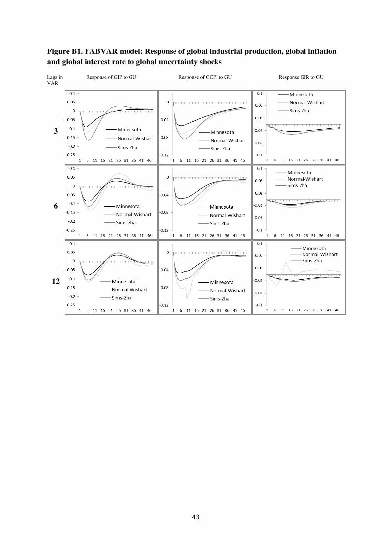
8.1. The effects of global uncertainty shocks on the economy in the FABVAR model

Figure B1 shows the impact of one-standard-deviation global uncertainty shocks on

global industrial production growth, CPI inflation and interest rate for the FABVAR model,

with vector of endogenous variables 𝑦𝑡 = (∆(𝐺𝐼𝑃𝑡), ∆(𝐺𝐶𝑃𝐼𝑡), 𝐺𝐼𝑅𝑡, 𝐺𝑈𝑡 ). The model is

estimated with 3, 6 and 12 lags, as indicated on the left hand side of Figure B1. Each column

in Figure B1 shows the response of global interest rate, CPI inflation and industrial production

growth to global uncertainty shocks. The timing and magnitude of the responses to a one-time

global uncertainty shock in the economy in Figure B1 are very similar to the results in Figure

4 from the FAVAR model.

In brief, global uncertainty shocks are accompanied by a quick decline in global

industrial production growth that is most severe after 4 to 8 months. Global uncertainty shocks

are associated with a quick and sharp decline in global CPI, reaching the greatest levels of

decline after 6 to 12 months, depending on the number of lags and the prior adopted. Global

uncertainty shocks are associated with a decline in global interest rate that persists with the

greatest decline in the global interest rate observed over 16 to 20 months. The only exception

23

to the latter results for the impact of global uncertainty on the global interest rate is for the

FABVAR model with Sims-Zha prior, for which the decline in interest rate is greatest after 7

or 8 months and is reversed after 10 months.

8.2. Effects of global uncertainty and U.S. uncertainty shocks in the FABVAR model

The effects of global uncertainty and U.S. uncertainty shocks on the variables in the

FABVAR model are now presented. The vector of endogenous variables is a (𝑚 = 5) × 1

given by 𝑦𝑡 = (∆(𝐺𝐼𝑃𝑡), ∆(𝐺𝐶𝑃𝐼𝑡), 𝐺𝐼𝑅𝑡, 𝑈𝑆𝑈𝑡, 𝐺𝑈𝑡 ). The responses of global industrial

production, CPI and interest rate to global uncertainty shocks and to U.S. uncertainty shocks

are shown in the first and second rows of Figure B2, respectively.

The results for the responses to global uncertainty (after controlling for U.S.

uncertainty) are well defined for all priors and are very similar to the results obtained from the

FAVAR model shown in Figure 5. A one-standard-deviation shock to global uncertainty is

associated with decreases in global industrial production over 1 to 16 months, persistent

reductions in global CPI with the deepest decline over 3 to 12 months (depending on prior) and

continual reductions in the global interest rate with the most decline over 12 to 16 months

(depending on the prior).

The results for the responses to U.S. uncertainty after controlling for global uncertainty

are also similar to the results obtained from the FAVAR model shown in Figure 5, meaning

that they are small and ill defined. The results from the FABVAR model reinforce the finding

that global uncertainty shocks dominate U.S. uncertainty shocks in terms of their influence on

the global economy. The responses of global output, CPI and interest rate to U.S uncertainty

shocks are much smaller in absolute value than the negative responses of global output, CPI

and interest rate to global uncertainty shocks.

8.3. Financial vs. non-financial uncertainty shock in the FABVAR model

24

The impacts of financial and non-financial uncertainty shocks on the global

macroeconomic variables estimated from the FABVAR model are presented in Figure B3. The

vector of endogenous variables is 𝑦𝑡 = (∆(𝐺𝐼𝑃𝑡), ∆(𝐺𝐶𝑃𝐼𝑡), 𝐺𝐼𝑅𝑡, 𝐹𝐷𝐹𝑡 ∗ 𝐺𝑈𝑡𝑈𝑡, 𝐷𝑁𝐹𝑡 ∗𝐺𝑈𝑡), where the fifth and sixth variables are the global financial uncertainty and global non-

financial uncertainty components of global uncertainty. In the first and second rows of Figure

B3, the impact of financial and non-financial uncertainty shocks on global industrial

production, CPI and interest rate are shown. Results for the impacts of global financial and

non-financial uncertainty shocks are similar to those reported for the earlier FAVAR model (in

Figure 6).

The financial uncertainty shocks have a much larger impact on the absolute value than

the non-financial shocks in reducing global industrial production. The differences between the

responses of global CPI to global financial and non-financial uncertainty shocks persist in the

FABVAR estimation. Financial uncertainty shocks have a negative effect on global CPI, and

non-financial shocks have a positive effect. Declines in global interest are associated with both

global financial and non-financial uncertainty shocks, but now the effect of the financial shock

is persistently negative.

8.4. Effects of global uncertainty on domestic economies in the FABVAR model

Results for the impulse responses of domestic output, inflation and interest rate for the

largest economies from the FABVAR model appear in Figures B4 and B5 for developed or

developing economies, respectively. The endogenous variables in the FABVAR model

estimated are given by 𝑦𝑡 = (∆(𝐷𝐼𝑃𝑡), ∆(𝐷𝐶𝑃𝐼𝑡), 𝐷𝐼𝑅𝑡, 𝐷𝑈𝑡 , 𝐺𝑈𝑡) , where the first four

variables are output, CPI, interest rate and uncertainty for a large developed or developing

economy; the last variable is global uncertainty. Results are again similar to those reported for

the FAVAR model.

25

In Figures B4 and B5, the decline in the U.S. and China outputs are more muted in

response to increased global uncertainty than the outputs of the other countries. For most

countries, the responses of domestic inflation and the official interest to positive shocks to

global uncertainty are negative and consistent with the result for the negative effect of shocks

to global uncertainty on domestic output. The exceptions are Brazil, Mexico and Russia. For

Brazil, Mexico and Russia, an increase in global uncertainty is associated with increases in the

official interest rate, and for Mexico and Russia, an increase in global uncertainty is associated

with increases the official interest.

8.5. Ordering of variables

To accomplish an additional robustness check, we provided FAVAR models using a

reverse ordering of variables in the Cholesky-VAR system, as proposed by Bloom (2009);

these models can be found in the supplementary material section. These results confirm the

sign and statistical significance of the results from the main models estimated in the text.

8.6. Alternative measure of global uncertainty

In this section, we explore the use of three alternative measures of global uncertainty.

The first alternative measure proposed is the GDP-weighted index of country specific volatility

(also for the largest 15 economies). For this alternative measure, we weight each country of the

15 largest economies using GDP Purchase Power Parity (PPP) in U.S. dollars as reported by

the Wold Bank. The main drawback of this measure is that the intertemporal change in weights

can only be incorporated annually as this data is only available on an annual basis from the

World Bank.

A second alternative measure considered is for the largest 20 economies (rather than 15

economies) using the principal component analysis described in Equations 1 to 3. The

additional countries included in this measure are Indonesia, Iran, Thailand, Nigeria and Poland.

The stock market data for these countries is only available for a shorter span (generally from

26

the 1990s), and therefore the inclusion of these five countries only change the benchmark

measure of global uncertainty from 1990.

The third alternative measure is based on the notion from Jurado et al. (2015) that

uncertainty can be defined as the unforecastable component of a linear regression. In the spirit

of this definition, we consider the residual of the following equation as a measure of global

uncertainty: 𝐺𝑈𝑡 = 𝛽0 + 𝛽1𝐺𝑈𝑡+1 + 𝜖 (11)

where 𝐺𝑈𝑡 is the global uncertainty index from Equation 1 to 3, 𝐺𝑈𝑡+1 is the same index at

time 𝑡+1 and is considered the optimal forecast under the Efficient Market Hypothesis (EMH)

and 𝜖 is the residual or uncertainty measure.18

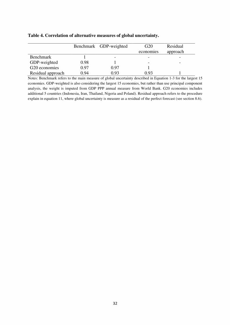
Table 4 reports the correlation coefficients of alternative measures of global

uncertainty. The correlations are very high amongst these four measures, ranging from 0.98 to

0.94. In results available from the authors, we show that either measure of global uncertainty

leads to very similar results in both the FAVAR and FABVAR models.

9. Conclusions

In this paper, we examine the impact of global uncertainty on the global economy and

on large developed and developing economies. This supplements the recent literature that has

analyzed the effects of uncertainty (either U.S. or global) on country-level macroeconomic

variables. Using principal component analysis of the stock market volatility indexes for the

largest 15 economies, a global uncertainty measure is identified. Taking advantage of the new

global database from DGEI from the Federal Reserve Bank of Dallas, we explore the impact

18 The EMH predicts that prices on traded assets (and/or future prices) already reflect all past publicly available information. Consequently, the residual of this Equation can be interpreted as uncertainty using Jurado et al (2015)’s rationale.

27

of global uncertainty on key global macroeconomic variables of major developed and

developing economies.

We find that global uncertainty shocks are associated with a sharp decline in global

industrial production, inflation and interest rate. The maximum decline of industrial production

and global inflation occurs six months after a global uncertainty shock, while the maximum

decline in global interest rate occurs after 16 months after a global uncertainty shock. At the

country level, global uncertainty shocks (even controlling for domestic uncertainty) reduce

outputs in most large developed and developing economies. Outputs from Russia, Brazil and

South Africa are most affected by global uncertainty shocks, while outputs from China and the

U.S. and U.K. are less responsive to these shocks.

We use existing knowledge on important global events to distinguish between financial

and non-financial uncertainty shocks. Our decomposition of global uncertainty shocks shows

that global financial uncertainty shocks are more important (for the global economy) than non-

financial uncertainty shocks. From 1981 to 2014, global financial uncertainty forecasts 18.26%

and 14.95% of the variation in global growth and global inflation, respectively, while non-

financial uncertainty shocks forecast only 7.75% and 2.15% of the variation in global growth

and global inflation, respectively.

References

Arellano, C., Bai, Y., and Kehoe, P. (2010). “Financial Markets and Fluctuations in Volatility.” Federal Reserve Bank of Minneapolis Working Paper. Bachmann, R., Elstner, S., and Sims, E.R. (2013). “Uncertainty and Economic Activity: Evidence from Business Survey Data.” American Economic Journal: Macroeconomics 5, 217-49. Baum, C. F., Caglaynan, M., and Talavera, O. (2010). “On the Sensitivity of Firms’ Investment to Cash Flow and Uncertainty.” Oxford Economic Papers 62, 286-306. Bekaert, G., Hoerova, M., and Duca, M.L. (2013). “Risk, Uncertainty and Monetary Policy.” Journal of Monetary Economics 60, 771-788.

28

Berger, T. and Herz, S. (2014). “Global Macroeconomic Uncertainty.” Working paper, available at https://www.gwu.edu/~forcpgm/BergerHerz_gmu.pdf. Bloom, N. (2009). “The Impact of Uncertainty Shocks.” Econometrica 77, 623-685. Bloom, N., Bond, S., and Van Reenen, J. (2007). “Uncertainty and Investment Dynamics.” Review of Economic Studies 74, 391-415. Bredin, D. and Fountas, S. (2009). “Macroeconomic Uncertainty and Performance in the European Union.” Journal of International Money and Finance 28, 972-986. Charemza, W., Díaz, C., and Makarova, S. (2015). “Conditional Term Structure of Inflation Forecast Uncertainty: The Copula Approach.” University of Leicester Working Paper No. 15/07. Christiano, L. J., Eichenbaum, M., and Evans, C. L. (2005). “Nominal Rigidities and the Dynamic Effects of a Shock to Monetary Policy.” Journal of Political Economy 113, 1-45. Delrio, S. (2016). “Estimating the Effects of Global Uncertainty in Open Economies.” Working paper, available at SSRN 2832727. Favero, C. (2009). “Uncertainty and the Tale of two Depressions: Let Eichengreen and O'Rourke meet Bloom.” VoxEU, 2009. Fernández-Villaverde, J., Guerrón-Quintana, P., Rubio-Ramírez, J. F. and Uribe, M. (2011). “Risk Matters: The Real Effects of Volatility Shocks.” American Economic Review 6, 2530–61 Gilchrist, S., Sim, J. W., and Zakrajsek, E. (2010). “Uncertainty, Financial Frictions, and Investment Dynamics.” Society for Economic Dynamics 2010 Meeting Paper 1285. Grossman, V., Mack, A., and Martinez-Garcia, E. (2014). “Database of global economic indicators (DGEI): a methodological note.” Globalization and Monetary Policy Institute Working Paper 166, Federal Reserve Bank of Dallas. Hirata, H., Kose, M. A., Otrok, C., Terrones, M. E. (2012). “Global House Price Fluctuations: Synchonization and Determinants.” NBER Working Paper 18362, available at http://www.nber.org/papers/w18362. Jurado, K., Ludvigson, S. C. and Ng, S. (2015). "Measuring Uncertainty." American Economic Review 105, 1177-1216. Knotek, E. S., and Khan, K. (2011). “How Do Households Respond to Uncertainty Shocks?” Federal Reserve Bank of Kansas City Economic Review 96, 5-34. Leduc, Sylvain and Zheng Liu (2015). “Uncertainty Shocks are Aggregate Demand Shocks.” Federal Reserve Bank of San Francisco, Working Paper 2012-10.

29

Leahy, J. V., and Whited, T.M. (1996). “The Effect of Uncertainty on Investment: Some Stylized Facts.” Journal of Money, Credit and Banking 28, 64-83. Mumtaz, H., and Theodoridis, K. (2014). “The international transmission of volatility shocks: an empirical analysis.” Journal of the European Economic Association 13, 512-533. Obstfeld, M., Shambaugh, J.C., and Taylor, A. M. (2009). “Financial Instability, Reserves, and Central Bank Swap Lines in the Panic of 2008.” American Economic Review 99, 480-86. Ozturk, E. O., and Sheng, X. S. (2016). “Measuring Global and Country-specific uncertainty.” Working paper, available at http://www.pramu.ac.uk/wp-content/uploads/2016/04/Ozturk-and-Sheng_Measuring-global-uncertainty.pdf. Rossi, B. and Sekhposyan, T. (2015). “Macroeconomic Uncertainty Indices Based on Nowcast and Forecast Error Distributions.” American Economic Review 105, 650-55. Shaghil, A., and Zlate, A. (2014). “Capital flows to emerging market economies: A brave new world?” Journal of International Money and Finance 48, 221-248.

30

Table 1. Correlation of the lag structure between global and the U.S. uncertainty (cross

correlogram)

Global, U.S. (-i) Global ,U.S.(+i) i lag lead .|++ | .|++| 0 0.165 0.165 .|| .|+++++++++| 1 0.001 0.889 .|| .|++| 2 0.023 0.218 .|+| .|| 3 0.049 -0.008 .|| .|+| 4 0.014 0.112 .|+| .|+| 5 0.155 0.108 .|| .|+| 6 0.036 0.051 .|| .|++| 7 -0.022 0.163 .|+| .|+| 8 0.060 0.101 .|| .| | 9 0.043 0.010 .|| .|+| 10 -0.012 0.085 .|| .|+| 11 -0.019 0.118 .|| .|| 12 -0.004 0.030

Note that in column 1 and 2 are only for optical view, + represents a value close to 0.1 correlation.

Table 2. Granger causality test between global and the U.S. uncertainty

Null Hypothesis: x does not Granger cause y

Granger test/Lags 1 3 6 12

Global uncertainty does not granger cause U.S. uncertainty

1479.01*** 496.04*** 237.05*** 119.05***

U.S. Uncertainty does not granger cause global uncertainty

0.58 3.57** 2.77** 1.02

Notes: ***, **, * indicates rejection of the null hypothesis at 1%, 5% and 10%, levels of significance respectively.

31

Table 3. Variance decomposition of global macroeconomic variables

a. Forecast error variance decomposition of global industrial production

Contribution from/months

Global IP Global CPI Global IR Financial uncertainty shock

Non-financial uncertainty shock

1 100.00*** 0.00 0.00 0.00 0.00 6 85.99*** 0.82 0.05 12.25*** 0.88 12 64.71*** 10.86* 0.83 18.95*** 4.66 18 52.48*** 19.78** 2.70** 17.26*** 7.78 24 51.21*** 20.51*** 3.43** 16.85*** 8.00 30 51.44*** 19.54*** 3.28** 18.11*** 7.63 36 50.71*** 19.75*** 3.46** 18.35*** 7.73 48 50.58*** 19.74*** 3.67** 18.26*** 7.75

Notes: ***, **, * indicates rejection of the null hypothesis at 1%, 5% and 10%, levels of significance respectively.

b. Forecast error variance decomposition of global CPI

Contribution from/months

Global IP Global CPI Global IR Financial uncertainty shock

Non-financial uncertainty shock

1 0.19 99.81*** 0.00 0.00 0.00 6 7.02 85.77*** 0.24 5.44* 1.53 12 14.95** 66.66*** 2.75 13.02** 2.63 18 18.95** 54.21*** 8.02* 16.64** 2.17 24 18.90*** 47.68*** 14.35** 16.88** 2.19 30 18.02*** 44.15*** 19.52** 16.08** 2.22 36 17.45*** 41.99*** 22.98** 15.40** 2.18 48 17.31*** 40.40*** 25.20** 14.95** 2.15

Notes: ***, **, * indicates rejection of the null hypothesis at 1%, 5% and 10%, levels of significance respectively.

c. Forecast error variance decomposition of global interest rate

Contribution from/months

Global IP Global CPI Global IR Financial uncertainty shock

Non-financial uncertainty shock

1 2.86 0.03 97.11*** 0.00 0.00 6 4.20 0.09 95.24*** 0.34 0.14 12 6.95 0.07 91.06*** 0.94 0.99 18 9.21 0.10 87.51*** 1.72 1.46 24 10.36 0.23 85.21*** 2.28 1.92 30 10.64 0.36 84.27*** 2.49 2.24 36 10.62* 0.41 84.03*** 2.53 2.41 48 10.60* 0.42 83.97*** 2.52 2.49

Notes: ***, **, * indicates rejection of the null hypothesis at 1%, 5% and 10%, levels of significance respectively.

32

Table 4. Correlation of alternative measures of global uncertainty.

Benchmark GDP-weighted G20 economies

Residual approach

Benchmark 1 - - - GDP-weighted 0.98 1 - - G20 economies 0.97 0.97 1 Residual approach 0.94 0.93 0.93 1

Notes: Benchmark refers to the main measure of global uncertainty described in Equation 1-3 for the largest 15

economies. GDP-weighted is also considering the largest 15 economies, but rather than use principal component

analysis, the weight is imputed from GDP PPP annual measure from World Bank. G20 economies includes

additional 5 countries (Indonesia, Iran, Thailand, Nigeria and Poland). Residual approach refers to the procedure

explain in equation 11, where global uncertainty is measure as a residual of the perfect forecast (see section 8.6).

33

Figure 1. Global volatility index: 12-month moving average standard deviation

Figure 2. U.S. volatility index: 12-month moving average standard deviation

Figure 3. Global and U.S. volatility indices scaled so that mean volatilities are equal.

34

Figure 4. Responses of global industrial production, inflation and interest rate to global

uncertainty shocks

Lags in VAR

Response of GIP to GU Response of GCPI to GU Response GIR to GU

3

6

12

Notes: The dashed lines represent a one standard error confidence band around the estimates of the coefficients of the impulse response functions. The confidence bands are obtained using Monte Carlo integration as described by Sims (1980), where 5000 draws were used from the asymptotic distribution of the VAR coefficient.

35

Figure 5. Responses of global variables to U.S. and global uncertainty shocks

Uncertainty

Shocks Response of GIP Response of GCPI Response GIR

Notes: to conserve space we only report results when 6 lags are specified in the FAVAR system. Results for 3 and

12 lags are available from the authors upon request.

Figure 6. Responses of global variables to financial and non-financial uncertainty shocks

Uncertainty

Shocks Response of GIP Response of GCPI Response GIR

Note that to conserve space we only report results when 6 lags are specified in the FAVAR system. Results for 3

and 12 lags are available from the authors upon request.

G L O B A L

U S

F I N A N C I A L

NO N - F I N A N C I A L

36

Figure 7a. Responses of large developed economies to global uncertainty shocks

Notes: The dashed lines represent a one standard error confidence band around the estimates of the coefficients of the impulse response functions. The confidence bands are obtained using Monte Carlo integration as described by Sims (1980), where 5000 draws were used from the asymptotic distribution of the VAR coefficient.

Response of Domestic Output Response of Domestic CPI Response Domestic IR

UK

I TALY

JAPAN

GERMANY

US

FRANCE

37

Figure 7b. Responses of large developing economies to global uncertainty shocks

Notes: The dashed lines represent a one standard error confidence band around the estimates of the coefficients

of the impulse response functions. The confidence bands are obtained using Monte Carlo integration as described

by Sims (1980), where 5000 draws were used from the asymptotic distribution of the VAR coefficient.

Response of Domestic Output Response of Domestic CPI Response Domestic IR

CHINA

INDIA

B R AZ I L

RUSS IA

S. AFR I CA

MEXI CO

38

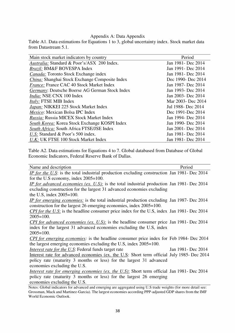
Appendix A: Data Appendix

Table A1. Data estimations for Equations 1 to 3, global uncertainty index. Stock market data from Datastream 5.1.

Main stock market indicators by country Period Australia: Standard & Poor’s/ASX 200 Index. Jan 1981- Dec 2014 Brazil: BM&F BOVESPA Index Jan 1991- Dec 2014 Canada: Toronto Stock Exchange index Jan 1981- Dec 2014 China: Shanghai Stock Exchange Composite Index Dec 1990- Dec 2014 France: France CAC 40 Stock Market Index Jan 1987- Dec 2014 Germany: Deutsche Boerse AG German Stock Index Jan 1993- Dec 2014 India: NSE CNX 100 Index Jan 2003- Dec 2014 Italy: FTSE MIB Index Mar 2003- Dec 2014 Japan: NIKKEI 225 Stock Market Index Jul 1988- Dec 2014 Mexico: Mexican Bolsa IPC Index Dec 1991-Dec 2014 Russia: Russia MICEX Stock Market Index Jan 1994- Dec 2014 South Korea: Korea Stock Exchange KOSPI Index Jan 1990- Dec 2014 South Africa: South Africa FTSE/JSE Index Jan 2001- Dec 2014 U.S: Standard & Poor’s 500 index. Jan 1981- Dec 2014 U.K: UK FTSE 100 Stock Market Index Jan 1981- Dec 2014 Table A2. Data estimations for Equations 4 to 7. Global databased from Database of Global Economic Indicators, Federal Reserve Bank of Dallas. Name and description Period IP for the U.S: is the total industrial production excluding construction for the U.S economy, index 2005=100.

Jan 1981- Dec 2014

IP for advanced economies (ex. U.S): is the total industrial production excluding construction for the largest 31 advanced economies excluding the U.S, index 2005=100.

Jan 1981- Dec 2014

IP for emerging economies: is the total industrial production excluding construction for the largest 26 emerging economies, index 2005=100.

Jan 1987- Dec 2014

CPI for the U.S: is the headline consumer price index for the U.S, index 2005=100.

Jan 1981- Dec 2014

CPI for advanced economies (ex. U.S): is the headline consumer price index for the largest 31 advanced economies excluding the U.S, index 2005=100.

Jan 1981- Dec 2014

CPI for emerging economies: is the headline consumer price index for the largest emerging economies excluding the U.S, index 2005=100.

Feb 1984- Dec 2014

Interest rate for the U.S: Federal funds target rate Jan 1981- Dec 2014

Interest rate for advanced economies (ex. the U.S: Short term official policy rate (maturity 3 months or less) for the largest 31 advanced economies excluding the U.S.

July 1985- Dec 2014

Interest rate for emerging economies (ex. the U.S): Short term official policy rate (maturity 3 months or less) for the largest 26 emerging economies excluding the U.S.

Jan 1981- Dec 2014

Notes: Global indicators for advanced and emerging are aggregated using U.S trade weights (for more detail see: Grossman, Mack and Martinez-Garcia). The largest economies according PPP-adjusted GDP shares from the IMF World Economic Outlook.

39

Table A3. Chronology of the global financial crisis events

Period Event

September 13, 2007 Northern Rock has sought emergency funding from the Bank of England in its capacity as "lender of last resort"

February 17, 2008 The U.K. government announces that struggling Northern Rock is to be nationalised for a temporary period.

July 14, 2008 Financial authorities in U.S. step in to assist America's two largest lenders, Fannie Mae and Freddie Mac, owners or guarantors of 5 trillion worth of home loans.

September 15, 2008 Wall Street bank Lehman Brothers (U.S.) files for Chapter 11 bankruptcy protection and another US bank, Merrill Lynch, is taken over by the Bank of America.

October 20, 2008 The U.S. government took control of AIG. The U.S. The federal government to take control of the company and guarantee to loan it up to $85 billion.

Table A4. Dummy variables for financial and non-financial shocks for Equation 9

Global financial shocks above 1.65 SD Global non-financial shocks above 1.65 SD Shock

Monthly dummy Shock Monthly dummy

Black Monday February to July 1987 September 11 terrorist attack

September to November 2001

Russian sovereign debt crisis

May and June 1997 Gulf War II

May to August 2002

Global financial crisis

September 2007 to November 2008

The dummy variables only take the value of 1 when the identified shock exceeds 1.65 standard deviations following Bloom (2009).

40

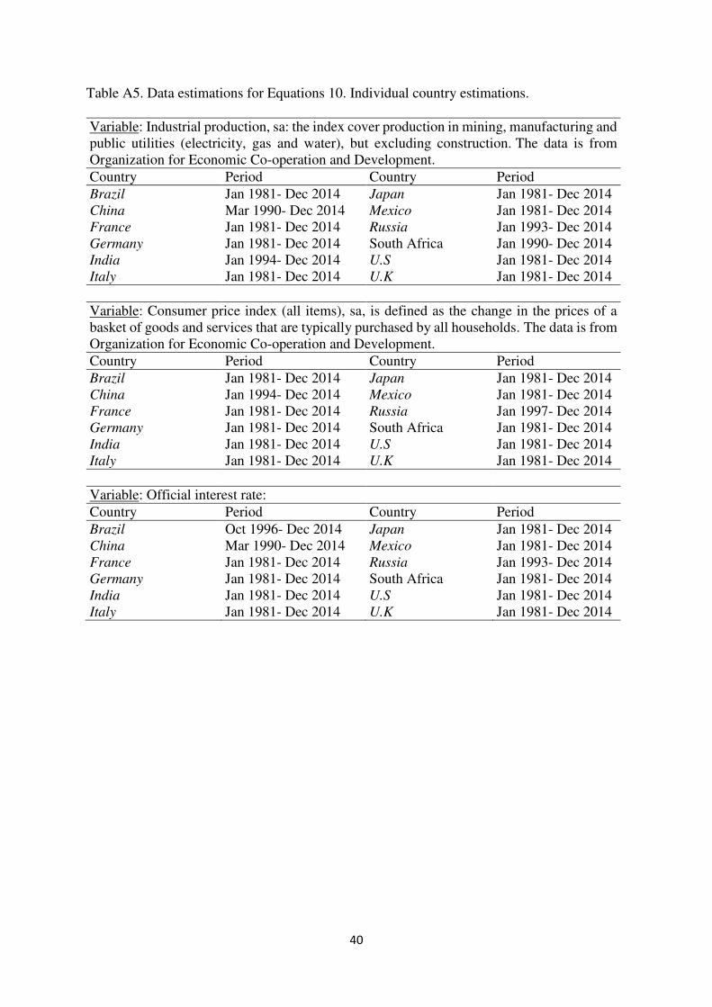
Table A5. Data estimations for Equations 10. Individual country estimations.

Variable: Industrial production, sa: the index cover production in mining, manufacturing and public utilities (electricity, gas and water), but excluding construction. The data is from Organization for Economic Co-operation and Development. Country Period Country Period Brazil Jan 1981- Dec 2014 Japan Jan 1981- Dec 2014

China Mar 1990- Dec 2014 Mexico Jan 1981- Dec 2014

France Jan 1981- Dec 2014 Russia Jan 1993- Dec 2014

Germany Jan 1981- Dec 2014 South Africa Jan 1990- Dec 2014

India Jan 1994- Dec 2014 U.S Jan 1981- Dec 2014

Italy Jan 1981- Dec 2014 U.K Jan 1981- Dec 2014

Variable: Consumer price index (all items), sa, is defined as the change in the prices of a basket of goods and services that are typically purchased by all households. The data is from Organization for Economic Co-operation and Development. Country Period Country Period Brazil Jan 1981- Dec 2014 Japan Jan 1981- Dec 2014

China Jan 1994- Dec 2014 Mexico Jan 1981- Dec 2014

France Jan 1981- Dec 2014 Russia Jan 1997- Dec 2014

Germany Jan 1981- Dec 2014 South Africa Jan 1981- Dec 2014

India Jan 1981- Dec 2014 U.S Jan 1981- Dec 2014

Italy Jan 1981- Dec 2014 U.K Jan 1981- Dec 2014

Variable: Official interest rate: Country Period Country Period Brazil Oct 1996- Dec 2014 Japan Jan 1981- Dec 2014

China Mar 1990- Dec 2014 Mexico Jan 1981- Dec 2014

France Jan 1981- Dec 2014 Russia Jan 1993- Dec 2014

Germany Jan 1981- Dec 2014 South Africa Jan 1981- Dec 2014

India Jan 1981- Dec 2014 U.S Jan 1981- Dec 2014

Italy Jan 1981- Dec 2014 U.K Jan 1981- Dec 2014

41

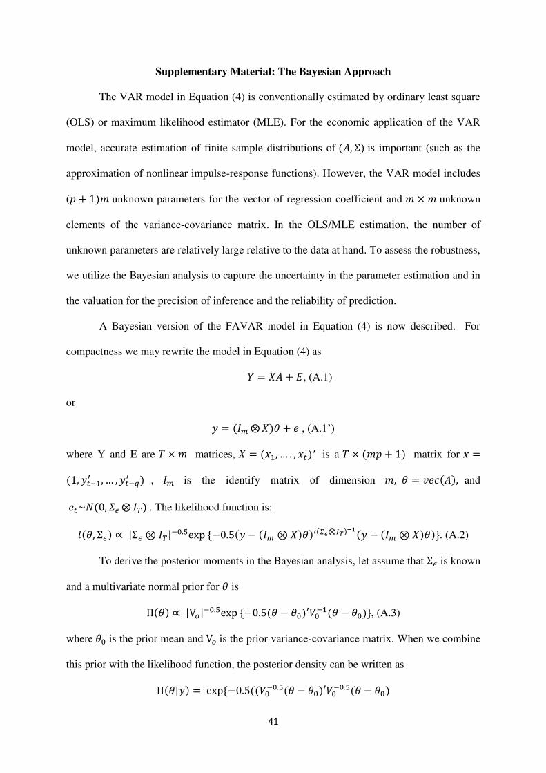
Supplementary Material: The Bayesian Approach

The VAR model in Equation (4) is conventionally estimated by ordinary least square

(OLS) or maximum likelihood estimator (MLE). For the economic application of the VAR

model, accurate estimation of finite sample distributions of (𝐴, Σ) is important (such as the

approximation of nonlinear impulse-response functions). However, the VAR model includes

(𝑝 + 1)𝑚 unknown parameters for the vector of regression coefficient and 𝑚 × 𝑚 unknown

elements of the variance-covariance matrix. In the OLS/MLE estimation, the number of

unknown parameters are relatively large relative to the data at hand. To assess the robustness,

we utilize the Bayesian analysis to capture the uncertainty in the parameter estimation and in

the valuation for the precision of inference and the reliability of prediction.

A Bayesian version of the FAVAR model in Equation (4) is now described. For

compactness we may rewrite the model in Equation (4) as 𝑌 = 𝑋𝐴 + 𝐸, (A.1)

or 𝑦 = (𝐼𝑚 ⨂𝑋)𝜃 + 𝑒 , (A.1’)

where Y and E are 𝑇 × 𝑚 matrices, 𝑋 = (𝑥1, … . , 𝑥𝑡)′ is a 𝑇 × (𝑚𝑝 + 1) matrix for 𝑥 =(1, 𝑦𝑡−1′ , … , 𝑦𝑡−𝑞′ ) , 𝐼𝑚 is the identify matrix of dimension 𝑚, 𝜃 = 𝑣𝑒𝑐(𝐴), and 𝑒𝑡~𝑁(0, 𝛴𝜖 ⨂𝐼𝑇) . The likelihood function is: 𝑙(𝜃, Σ𝜖) ∝ |Σ𝜖 ⊗ 𝐼𝑇|−0.5exp {−0.5(𝑦 − (𝐼𝑚 ⊗ 𝑋)𝜃)′(𝛴𝜖⊗𝐼𝑇)−1(𝑦 − (𝐼𝑚 ⊗ 𝑋)𝜃)}. (A.2)

To derive the posterior moments in the Bayesian analysis, let assume that Σ𝜖 is known

and a multivariate normal prior for 𝜃 is Π(𝜃) ∝ |V𝑜|−0.5exp {−0.5(𝜃 − 𝜃0)′𝑉0−1(𝜃 − 𝜃0)}, (A.3)

where 𝜃0 is the prior mean and V𝑜 is the prior variance-covariance matrix. When we combine

this prior with the likelihood function, the posterior density can be written as Π(𝜃|𝑦) = exp {−0.5((𝑉0−0.5(𝜃 − 𝜃0)′𝑉0−0.5(𝜃 − 𝜃0)

42

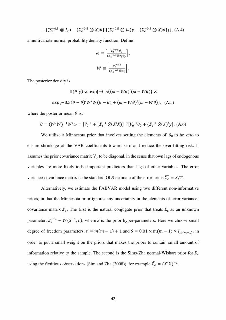
+{(Σ𝜖−0.5 ⊗ 𝐼𝑇) − (𝛴𝜖−0.5 ⊗ 𝑋)𝜃}′{(𝛴𝜖−0.5 ⊗ 𝐼𝑇)𝑦 − (𝛴𝜖−0.5 ⊗ 𝑋)𝜃})} , (A.4)

a multivariate normal probability density function. Define 𝜔 ≡ [ 𝑉0−0.5𝜃0(𝛴𝜖−0.5⊗𝐼𝑇)𝑦] , 𝑊 ≡ [ 𝑉0̅−0.5(𝛴𝜖−0.5⊗𝑋)] .

The posterior density is Π(𝜃|𝑦) ∝ exp {−0.5((𝜔 − 𝑊𝜃)′(𝜔 − 𝑊𝜃)} ∝ 𝑒𝑥𝑝 {−0.5(𝜃 − �̅�)′𝑊′𝑊(𝜃 − �̅�) + (𝜔 − 𝑊�̅�)′(𝜔 − 𝑊�̅�)}, (A.5)

where the posterior mean �̅� is: �̅� = (𝑊′𝑊)−1𝑊′𝜔 = [𝑉0−1 + (𝛴𝜖−1 ⊗ 𝑋′𝑋)]−1[𝑉0−1𝜃0 + (𝛴𝜖−1 ⊗ 𝑋)′𝑦] . (A.6)

We utilize a Minnesota prior that involves setting the elements of 𝜃0 to be zero to

ensure shrinkage of the VAR coefficients toward zero and reduce the over-fitting risk. It

assumes the prior covariance matrix V𝑜 to be diagonal, in the sense that own lags of endogenous

variables are more likely to be important predictors than lags of other variables. The error

variance-covariance matrix is the standard OLS estimate of the error terms Σ�̂� = 𝑆/𝑇.

Alternatively, we estimate the FABVAR model using two different non-informative

priors, in that the Minnesota prior ignores any uncertainty in the elements of error variance-

covariance matrix 𝛴𝜖 . The first is the natural conjugate prior that treats 𝛴𝜖 as an unknown

parameter, 𝛴𝜖−1 ∼ 𝑊(𝑆−1, 𝑣), where 𝑆 is the prior hyper-parameters. Here we choose small

degree of freedom parameters, 𝑣 = 𝑚(𝑚 − 1) + 1 and 𝑆 = 0.01 × 𝑚(𝑚 − 1) × 𝐼𝑚(𝑚−1), in

order to put a small weight on the priors that makes the priors to contain small amount of

information relative to the sample. The second is the Sims-Zha normal-Wishart prior for 𝛴𝜖

using the fictitious observations (Sim and Zha (2008)), for example Σ�̂� = (𝑋′𝑋)−1.

43

Figure B1. FABVAR model: Response of global industrial production, global inflation

and global interest rate to global uncertainty shocks

Lags in VAR

Response of GIP to GU Response of GCPI to GU Response GIR to GU

3

6

12

44

Figure B2. FABVAR model: Responses of global variables to U.S and global uncertainty

shocks

Uncertainty Response of GIP to GU

Shocks

Response of GCPI to GU Response GIR to GU

G

L

O

B

A

L

U

S

Notes: To conserve space we only report results when 6 lags are specified in the FABVAR system. Results for 3

and 12 lags are available from the authors upon request.

Figure B3. FABVAR model: Responses of global variables to financial and non-financial

uncertainty shocks

Notes: To conserve space we only report results when 6 lags are specified in the FABVAR system. Results for 3

and 12 lags are available from the authors upon request.

Uncertainty Response of GIP to GU

Shocks

Response of GCPI to GU Response GIR to GU

F

I

N

A

N

C

I

A

L

N

O

N

-

F

I

N

A

N

C

I

A

L

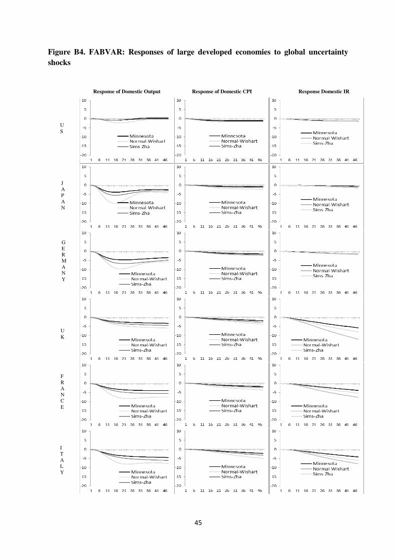
45

Figure B4. FABVAR: Responses of large developed economies to global uncertainty

shocks

Response of Domestic Output Response of Domestic CPI Response Domestic IR

UK

I TALY

JAPAN

GERMANY

US

FRANCE

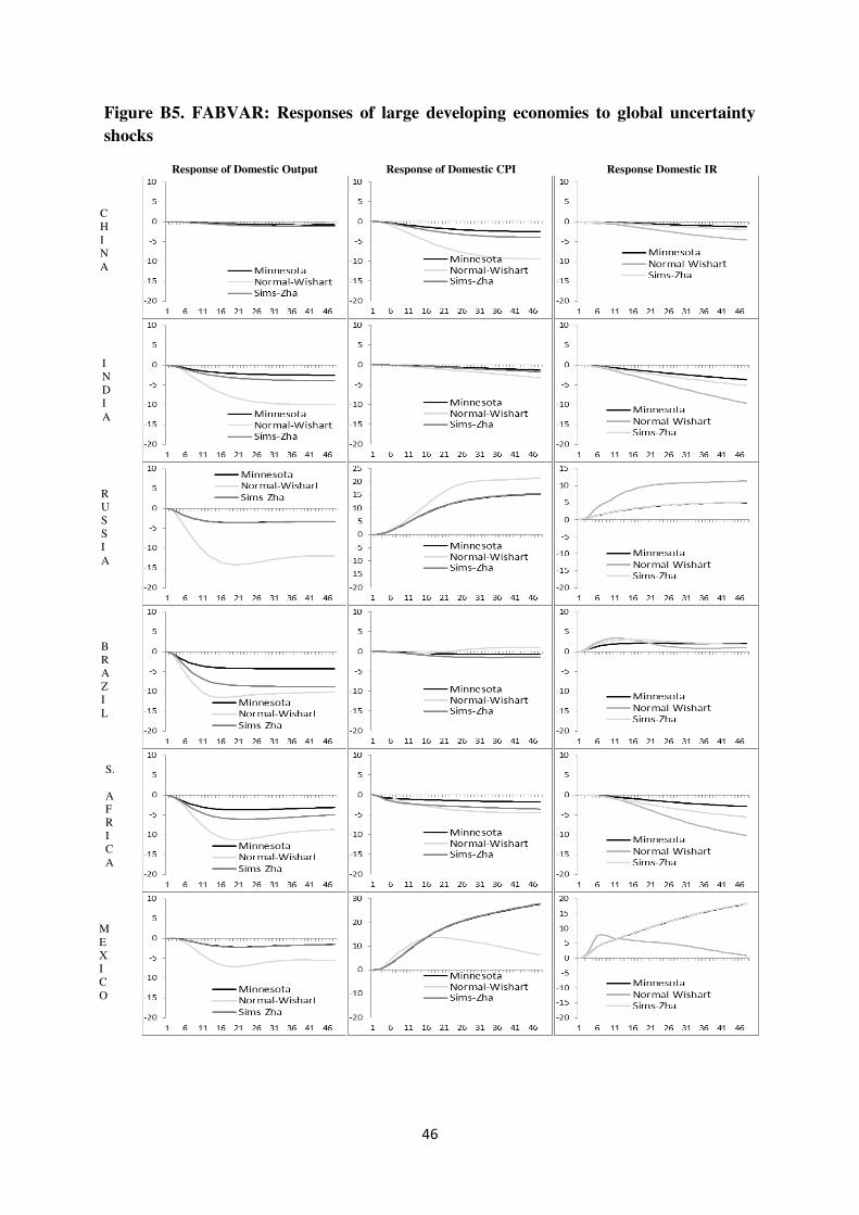
46

Figure B5. FABVAR: Responses of large developing economies to global uncertainty

shocks

Response of Domestic Output Response of Domestic CPI Response Domestic IR

CHINA

INDIA

B R AZ I L

RUSS IA

S. AFR I CA

MEXI CO

47

Discussion

1. The effects of global uncertainty shocks on the economy in the FABVAR model

Figure B1 shows the impact of one standard deviation global uncertainty shocks on

global industrial production growth, global CPI inflation and global interest rate for the

FABVAR model, with vector of endogenous variables 𝑦𝑡 = (∆(𝐺𝐼𝑃𝑡),∆(𝐺𝐶𝑃𝐼𝑡), 𝐺𝐼𝑅𝑡, 𝐺𝑈𝑡 ). The model is estimated with 3, 6 and 12 lags, as indicated on the left

hand side of Figure B1. Each column in Figure B1 shows the response of global interest rate,

global CPI inflation and global industrial production growth to global uncertainty shocks. The

timing and magnitude of the responses to a one-time global uncertainty shock in the economy

in Figure B1 are very similar to the results in Figure 4 from the FAVAR model.

In brief, global uncertainty shocks are accompany a quick decline in global industrial

production growth that is most severe after 4 to 8 months. Global uncertainty shocks are

associated with a quick and sharp decline in global CPI reaching the greatest levels of decline

after 6 to 12 months, depending on the number of lags and the prior adopted. Global uncertainty

shocks are associated with a decline in global interest rate that persists, with the greatest decline

in the global interest rate observed over 16 to 20 months. The only exception to the latter results

for the impact of global uncertainty on the global interest rate is for the FABVAR model with

Sims-Zha prior, for which case the decline in interest rate is greatest after 7 or 8 months and is

reversed after 10 months.

2. Effects of global uncertainty and U.S. uncertainty shocks in the FABVAR model

The effects of global uncertainty and U.S. uncertainty shocks on the variables in the

FABVAR model are now presented. The vector of endogenous variables is a (𝑚 = 5) × 1

given by 𝑦𝑡 = (∆(𝐺𝐼𝑃𝑡), ∆(𝐺𝐶𝑃𝐼𝑡), 𝐺𝐼𝑅𝑡, 𝑈𝑆𝑈𝑡, 𝐺𝑈𝑡 ). The responses of global industrial

production, CPI and interest rate to global uncertainty shocks and to U.S. uncertainty shocks

are shown in the first and second rows of Figure B2 respectively.

48

The results for the responses to global uncertainty (after controlling for U.S.

uncertainty) are well defined for all priors and very similar to the results obtained from the

FAVAR model shown in Figure 5. A one-standard deviation shock to global uncertainty is

associated with decreases in global industrial production over 1 to 16 months, persistent

reductions in global CPI with the deepest decline over 3 to 12 months (depending on prior),

and continual reductions in the global interest rate with the most decline over 12 to 16 months

(depending on prior).

The results for the responses to U.S. uncertainty after controlling for global uncertainty

are also similar to the results obtained from the FAVAR model shown in Figure 5, in that they

are small and ill defined. The results from the FABVAR model reinforce the finding that global

uncertainty shocks dominate U.S. uncertainty shocks in terms of influence on the global

economy. The responses of global output, CPI and interest rate to U.S uncertainty shocks are

much smaller in absolute value than the negative responses of global output, CPI and interest

rate to global uncertainty shocks.

3. Financial vs. non-financial uncertainty shock in the FABVAR model

The impacts of financial and non-financial uncertainty shocks on the global

macroeconomic variables estimated from the FABVAR model are presented in Figure B3. The

vector of endogenous variables is 𝑦𝑡 = (∆(𝐺𝐼𝑃𝑡), ∆(𝐺𝐶𝑃𝐼𝑡), 𝐺𝐼𝑅𝑡, 𝐹𝐷𝑡 ∗ 𝐺𝑈𝑡 , 𝐷𝑁𝐹𝑡 ∗𝐺𝑈𝑡), where the fifth and sixth variables are the global financial uncertainty and global non-

financial uncertainty components of global uncertainty. In the first and second rows of Figure

B3 the impact of financial and non-financial uncertainty shocks on global industrial production,

CPI and interest rate are shown. Results for the impacts of global financial and non-financial

uncertainty shocks are similar to those reported for the FAVAR model earlier (in Figure 6).

The financial uncertainty shocks have a much larger impact in absolute value than the

non-financial shocks in reducing global industrial production. The differences between the

49

responses of global CPI to global financial and non-financial uncertainty shocks persist in the

FABVAR estimation. Financial uncertainty shocks have a negative effect on global CPI and

non-financial shocks have a positive effect. Decline in global interest is associated with both

global financial and non-financial uncertainty shocks, but now the effect of the financial shock

is persistently negative.

4. Effects of global uncertainty on domestic economies in the FABVAR model.

Results for the impulse responses of domestic output, domestic inflation and domestic

interest rate for the largest economies from the FABVAR model appear in Figures B4 and B5

for developed or developing economy respectively. The endogenous variables in the FABVAR

model estimated are given by 𝑦𝑡 = (∆(𝐷𝐼𝑃𝑡), ∆(𝐷𝐶𝑃𝐼𝑡), 𝐷𝐼𝑅𝑡, 𝐷𝑈𝑡 , 𝐺𝑈𝑡), where the first four

variables are output, CPI, interest rate and uncertainty for a large developed or developing

economy and the last variable is global uncertainty. Results are again similar to those reported

for the FAVAR model.

In Figures B4 and B5 the decline in the outputs of the US and of China are more muted

in response to increased global uncertainty than are the outputs of the other countries. For most

countries, the responses of domestic inflation and the official interest to positive shocks to

global uncertainty are negative and consistent with the result for the negative effect of shocks

to global uncertainty on domestic output. The exceptions are again Brazil, Mexico and Russia.

For Brazil, Mexico and Russia, an increase in global uncertainty is associated with increases

the official interest rate, and Mexico and Russia an increase in global uncertainty is associated

with increases the official interest.