Zoi Vrontisi, Alban Kitous, Bert Saveyn,

Toon Vandyck

Impact of low oil prices on the EU economy

2015

EUR 27537 EN

This publication is a Technical report by the Joint Research Centre, the European Commission’s in-house science

service. It aims to provide evidence-based scientific support to the European policy-making process. The scientific

output expressed does not imply a policy position of the European Commission. Neither the European

Commission nor any person acting on behalf of the Commission is responsible for the use which might be made

of this publication.

JRC Science Hub

https://ec.europa.eu/jrc

JRC98188

EUR 27537 EN

ISBN 978-92-79-52769-2

ISSN 1831-9424

doi:10.2791/222885

© European Union, 2015

Reproduction is authorised provided the source is acknowledged.

All images © European Union 2015, except: Cover picture: © Fotolia.com – Edelweis.

How to cite: Vrontisi, Z., Kitous, A., Saveyn, B., and Vandyck, T. (2015). Impact of low oil prices on the EU

economy. JRC Technical Reports. EUR 27537 EN

2

Table of contents

Acknowledgements ................................................................................................ 3

Abstract ............................................................................................................... 4

1. Recent Evolutions of Crude Oil Price .................................................................. 5

2. Economic impact of low oil prices ...................................................................... 7

2.1 The role of oil in the EU28 economies ........................................................... 8

2.2 Scenario definition ..................................................................................... 9

2.3 Results ................................................................................................... 10

3. Potential short-term evolution of the oil price ................................................... 15

3.1 Scenarios ................................................................................................ 15

3.2 Impact of oil demand and oil imports .......................................................... 17

4. Conclusions and Caveats ............................................................................... 19

References ......................................................................................................... 20

List of figures ...................................................................................................... 21

List of tables ....................................................................................................... 22

3

Acknowledgements

The authors are grateful for the comments received from the colleagues of DG ENER and

DG JRC on earlier versions of the analysis.

4

Abstract

The report describes the importance of oil for the EU economy and analyses the potential

economic effects that current low oil prices since mid-2014 may have in the EU28

economy. Further it assesses how the current oil price decrease may evolve up to 2020

and the consequences for global oil consumption. The analysis shows that a decrease of

the oil price from US$100 to US$50 may lead to a GDP gain of about 0.7%, both on a

global level and in the EU28, driven by private consumption and investment. The global

gains are not evenly distributed. Net oil importing countries gain, whereas oil exporting

countries lose. The analysis mainly focuses on the EU28 and it shows that the more oil-

intensive countries and sectors gain more than the rest of the economy. A 50% decrease

of the oil price may generate up to 3 million additional jobs (1.3% of the total labour

force). Interestingly, oil-intensive sectors do not necessarily improve their

competitiveness vis-à-vis their competitors in other regions, as non-EU producers may

be less energy efficient and therefore benefit more from low oil prices.

5

1. Recent Evolutions of Crude Oil Price

This report describes the importance of oil (imports) for the EU economy and analyzes

the potential economic effects of the lower oil price in the EU28. Further it assesses how

the current oil price decrease may evolve up to 2020 and the consequences for global oil

consumption.

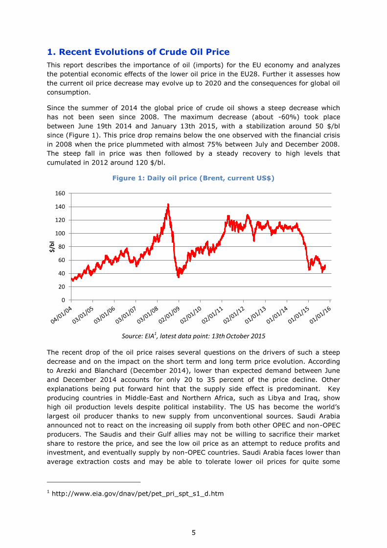
Since the summer of 2014 the global price of crude oil shows a steep decrease which

has not been seen since 2008. The maximum decrease (about -60%) took place

between June 19th 2014 and January 13th 2015, with a stabilization around 50 $/bl

since (Figure 1). This price drop remains below the one observed with the financial crisis

in 2008 when the price plummeted with almost 75% between July and December 2008.

The steep fall in price was then followed by a steady recovery to high levels that

cumulated in 2012 around 120 $/bl.

Figure 1: Daily oil price (Brent, current US$)

Source: EIA1, latest data point: 13th October 2015

The recent drop of the oil price raises several questions on the drivers of such a steep

decrease and on the impact on the short term and long term price evolution. According

to Arezki and Blanchard (December 2014), lower than expected demand between June

and December 2014 accounts for only 20 to 35 percent of the price decline. Other

explanations being put forward hint that the supply side effect is predominant. Key

producing countries in Middle-East and Northern Africa, such as Libya and Iraq, show

high oil production levels despite political instability. The US has become the world’s

largest oil producer thanks to new supply from unconventional sources. Saudi Arabia

announced not to react on the increasing oil supply from both other OPEC and non-OPEC

producers. The Saudis and their Gulf allies may not be willing to sacrifice their market

share to restore the price, and see the low oil price as an attempt to reduce profits and

investment, and eventually supply by non-OPEC countries. Saudi Arabia faces lower than

average extraction costs and may be able to tolerate lower oil prices for quite some

1 http://www.eia.gov/dnav/pet/pet_pri_spt_s1_d.htm

0

20

40

60

80

100

120

140

160

$/b

l

6

time. (The Economist, December 2014). For more details on the effects of the low oil

price for Saudi Arabia, we refer to IMF (2015b).

Moreover, various studies analyzed the correlation between the crude oil price and the

US$ exchange rate (for an overview see Table 3 in Breitenfellner and Crespo Cuaresma

(2008)). Over time, the negative relation between the U.S. dollar and the oil price,

driven by the exchange rate, seems to get increasing support. Indeed, between March

2014 and March 2015, the US dollar has appreciated with about 20% compared to the

Euro, to levels not seen for more than 10 years.

7

2. Economic impact of low oil prices

Oil consumption still remains one of the main pillars of our economies. The impact of the

observed price decrease will depend on the import dependency and the oil intensity of

the economy. In this respect, section 2.1 maps some descriptive statistics for EU

Member States. Section 2.2 briefly sets out the specifics of the oil price scenario studied.

The economic impact is reported in section 2.3 on a global scale and on the levels of the

EU28, the EU15 and the EU132. Moreover, the GDP impacts on a member state level are

graphically presented in order to track the impact variation across member states. The

macro-economic effects of the low oil price scenarios are analysed using the global GEM-

E3 model (see Box 1).

Box 1: GEM-E3 model

The macro-economic impacts of the oil price scenarios are analysed with the GEM-E3

model (www.gem-e3.net). It is a multi-region computable general equilibrium model

that covers the interactions between the economy, the energy system and the

environment. GEM-E3 covers the entire economy and can be used to evaluate

consistently the distributional effects of policies on the national accounts, investment,

consumption, public finance, foreign trade and employment for the various economic

sectors and agents across the countries. The model includes all 28 Member States of the

European Union and all major non-European countries. The whole economy is

represented in 21 economic sectors. The countries are linked through endogenous

bilateral trade. The GEM-E3 results are of comparative static nature, and reflect the

annual impact of imposing the lower oil price during a full year with the economy fully

adapting to the new situation. In other words, the lagged impacts of oil price changes

are observed to be spread over a couple of years, whereas in the GEM-E3 model they

are assumed to happen immediately in the same year. Further, this methodology also

assumes that the EU economy is in equilibrium. The model is calibrated using the GTAP

83 database.

The GEM-E3 model has been used to analyse the macro- economic effects of the climate,

energy and air quality policies to support DG CLIMA, DG ENER, and DG ENV (e.g.

SWD(2015) 17, SWD(2014) 15, SWD(2013)531, SWD(2013) 132). Ciscar et al. (2004)

and Maisonnave et al. (2012) use earlier versions of the GEM-E3 model to simulate the

impact of high oil prices (the latter focussing on the cross-relation with climate policies).

Kitous et al. (2013) analyse a number of scenarios of the 2012 Iran crisis and the

boycott imposed by the Western world.

2 I.e. the Member States that joined before and after 2004, respectively. The EU13

Member States are Lithuania, Estonia, Latvia, Poland, Czech Republic, Slovakia,

Hungary, Slovenia, Cyprus, Malta, Romania, Bulgaria, and Croatia. The EU15 Member

States are Belgium, the Netherlands, Luxemburg, Germany, Italy, France, Ireland,

United Kingdom, Denmark, Greece, Portugal, Spain, Austria, Sweden and Finland. 3 https://www.gtap.agecon.purdue.edu/

8

2.1 The role of oil in the EU28 economies

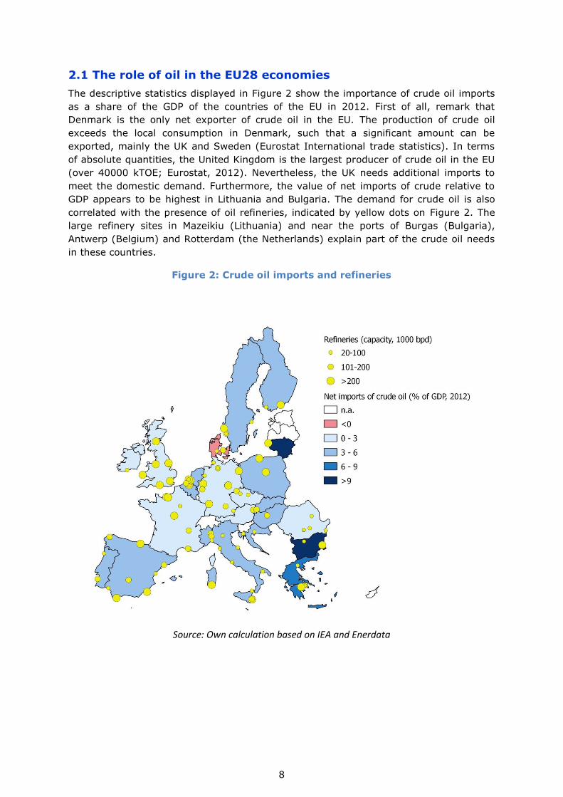
The descriptive statistics displayed in Figure 2 show the importance of crude oil imports

as a share of the GDP of the countries of the EU in 2012. First of all, remark that

Denmark is the only net exporter of crude oil in the EU. The production of crude oil

exceeds the local consumption in Denmark, such that a significant amount can be

exported, mainly the UK and Sweden (Eurostat International trade statistics). In terms

of absolute quantities, the United Kingdom is the largest producer of crude oil in the EU

(over 40000 kTOE; Eurostat, 2012). Nevertheless, the UK needs additional imports to

meet the domestic demand. Furthermore, the value of net imports of crude relative to

GDP appears to be highest in Lithuania and Bulgaria. The demand for crude oil is also

correlated with the presence of oil refineries, indicated by yellow dots on Figure 2. The

large refinery sites in Mazeikiu (Lithuania) and near the ports of Burgas (Bulgaria),

Antwerp (Belgium) and Rotterdam (the Netherlands) explain part of the crude oil needs

in these countries.

Figure 2: Crude oil imports and refineries

Source: Own calculation based on IEA and Enerdata

9

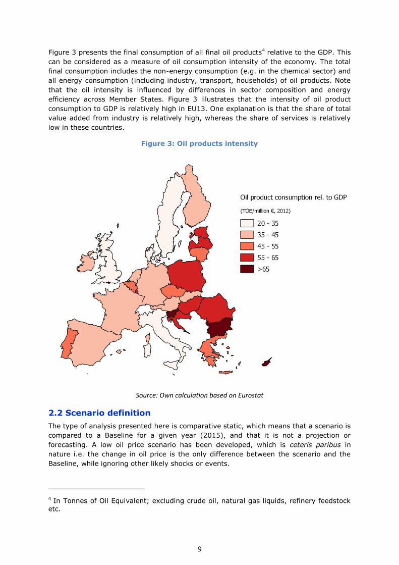
Figure 3 presents the final consumption of all final oil products4 relative to the GDP. This

can be considered as a measure of oil consumption intensity of the economy. The total

final consumption includes the non-energy consumption (e.g. in the chemical sector) and

all energy consumption (including industry, transport, households) of oil products. Note

that the oil intensity is influenced by differences in sector composition and energy

efficiency across Member States. Figure 3 illustrates that the intensity of oil product

consumption to GDP is relatively high in EU13. One explanation is that the share of total

value added from industry is relatively high, whereas the share of services is relatively

low in these countries.

Figure 3: Oil products intensity

Source: Own calculation based on Eurostat

2.2 Scenario definition

The type of analysis presented here is comparative static, which means that a scenario is

compared to a Baseline for a given year (2015), and that it is not a projection or

forecasting. A low oil price scenario has been developed, which is ceteris paribus in

nature i.e. the change in oil price is the only difference between the scenario and the

Baseline, while ignoring other likely shocks or events.

4 In Tonnes of Oil Equivalent; excluding crude oil, natural gas liquids, refinery feedstock

etc.

10

"Baseline": The "business-as-usual" development. Oil prices remain around US$ 100

per barrel in 2015.

"50% Scenario": This is the central scenario and assumes an oil price of US$ 50 per

barrel in 2015, which is 50% lower as compared to the baseline in dollar terms. Global

supply of crude oil is 7% higher than in the baseline.

2.3 Results

Table 1 reports the macro-economic impacts of the 50% Scenario. The Gross Domestic

Product (GDP) as well as its components5 are presented as a percentage difference from

the Baseline. The GDP increase for the EU28 and the World is about 0.7%. These results

are comparable with the analysis of Arezki and Blanchard (2014) who estimated, with a

different methodology, a GDP increase of about 0.6% for EU28 and 0.7% for the World,

for a permanent oil price decrease.

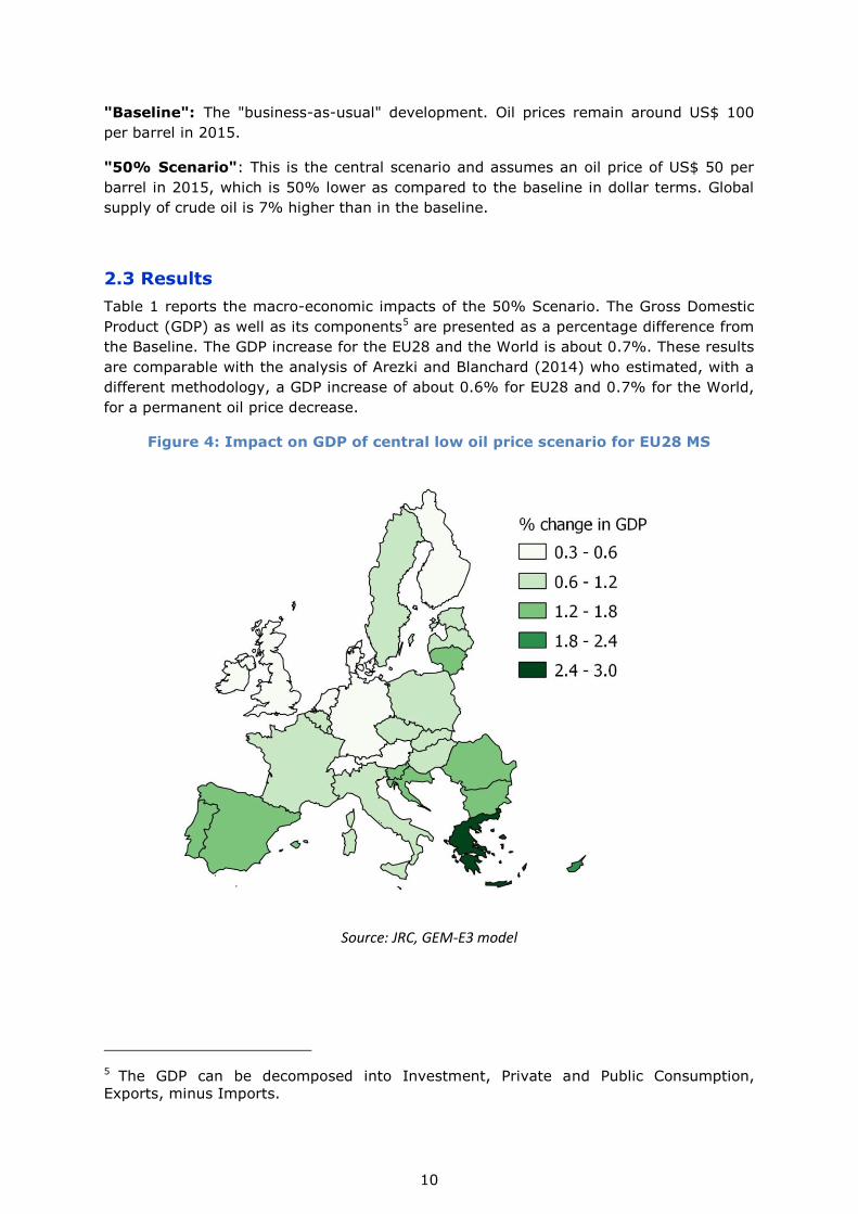
Figure 4: Impact on GDP of central low oil price scenario for EU28 MS

Source: JRC, GEM-E3 model

5 The GDP can be decomposed into Investment, Private and Public Consumption,

Exports, minus Imports.

11

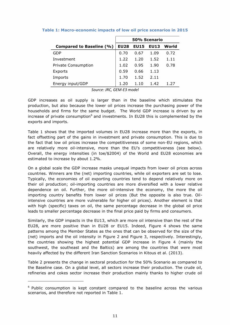
Table 1: Macro-economic impacts of low oil price scenarios in 2015

50% Scenario

Compared to Baseline (%) EU28 EU15 EU13 World

GDP 0.70 0.67 1.09 0.72

Investment 1.22 1.20 1.52 1.11

Private Consumption 1.02 0.95 1.90 0.78

Exports 0.59 0.66 1.13

Imports 1.70 1.52 2.11

Energy input/GDP 1.20 1.10 1.42 1.27

Source: JRC, GEM-E3 model

GDP increases as oil supply is larger than in the baseline which stimulates the

production, but also because the lower oil prices increase the purchasing power of the

households and firms for the same budget. The World GDP increase is driven by an

increase of private consumption6 and investments. In EU28 this is complemented by the

exports and imports.

Table 1 shows that the imported volumes in EU28 increase more than the exports, in

fact offsetting part of the gains in investment and private consumption. This is due to

the fact that low oil prices increase the competitiveness of some non-EU regions, which

are relatively more oil-intensive, more than the EU's competitiveness (see below).

Overall, the energy intensities (in toe/$2004) of the World and EU28 economies are

estimated to increase by about 1.2%.

On a global scale the GDP increase masks unequal impacts from lower oil prices across

countries. Winners are the (net) importing countries, while oil exporters are set to lose.

Typically, the economies of oil exporting countries tend to depend relatively more on

their oil production; oil-importing countries are more diversified with a lower relative

dependence on oil. Further, the more oil-intensive the economy, the more the oil

importing country benefits from lower oil prices (But the opposite is also true. Oil-

intensive countries are more vulnerable for higher oil prices). Another element is that

with high (specific) taxes on oil, the same percentage decrease in the global oil price

leads to smaller percentage decrease in the final price paid by firms and consumers.

Similarly, the GDP impacts in the EU13, which are more oil intensive than the rest of the

EU28, are more positive than in EU28 or EU15. Indeed, Figure 4 shows the same

patterns among the Member States as the ones that can be observed for the size of the

(net) imports and the oil intensity in Figure 2 and Figure 3, respectively. Interestingly,

the countries showing the highest potential GDP increase in Figure 4 (mainly the

southwest, the southeast and the Baltics) are among the countries that were most

heavily affected by the different Iran Sanction Scenarios in Kitous et al. (2013).

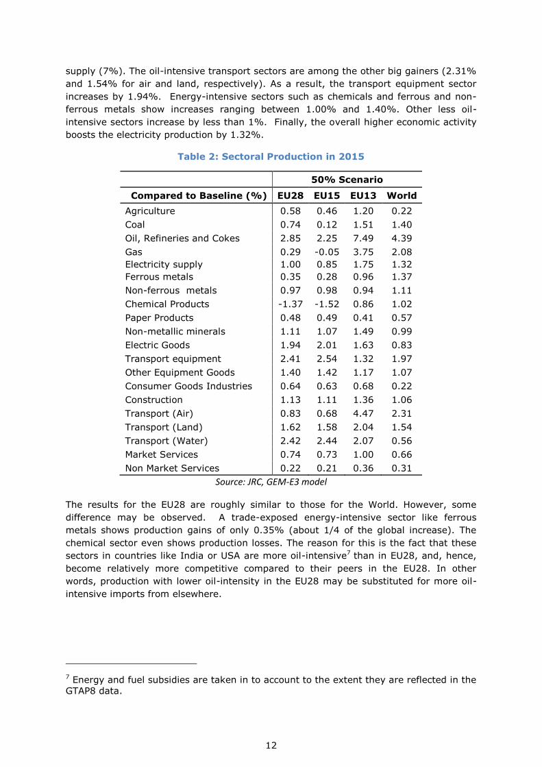
Table 2 presents the change in sectoral production for the 50% Scenario as compared to

the Baseline case. On a global level, all sectors increase their production. The crude oil,

refineries and cokes sector increase their production mainly thanks to higher crude oil

6 Public consumption is kept constant compared to the baseline across the various

scenarios, and therefore not reported in Table 1.

12

supply (7%). The oil-intensive transport sectors are among the other big gainers (2.31%

and 1.54% for air and land, respectively). As a result, the transport equipment sector

increases by 1.94%. Energy-intensive sectors such as chemicals and ferrous and non-

ferrous metals show increases ranging between 1.00% and 1.40%. Other less oil-

intensive sectors increase by less than 1%. Finally, the overall higher economic activity

boosts the electricity production by 1.32%.

Table 2: Sectoral Production in 2015

50% Scenario

Compared to Baseline (%) EU28 EU15 EU13 World

Agriculture 0.58 0.46 1.20 0.22

Coal 0.74 0.12 1.51 1.40

Oil, Refineries and Cokes 2.85 2.25 7.49 4.39

Gas 0.29 -0.05 3.75 2.08

Electricity supply 1.00 0.85 1.75 1.32

Ferrous metals 0.35 0.28 0.96 1.37

Non-ferrous metals 0.97 0.98 0.94 1.11

Chemical Products -1.37 -1.52 0.86 1.02

Paper Products 0.48 0.49 0.41 0.57

Non-metallic minerals 1.11 1.07 1.49 0.99

Electric Goods 1.94 2.01 1.63 0.83

Transport equipment 2.41 2.54 1.32 1.97

Other Equipment Goods 1.40 1.42 1.17 1.07

Consumer Goods Industries 0.64 0.63 0.68 0.22

Construction 1.13 1.11 1.36 1.06

Transport (Air) 0.83 0.68 4.47 2.31

Transport (Land) 1.62 1.58 2.04 1.54

Transport (Water) 2.42 2.44 2.07 0.56

Market Services 0.74 0.73 1.00 0.66

Non Market Services 0.22 0.21 0.36 0.31

Source: JRC, GEM-E3 model

The results for the EU28 are roughly similar to those for the World. However, some

difference may be observed. A trade-exposed energy-intensive sector like ferrous

metals shows production gains of only 0.35% (about 1/4 of the global increase). The

chemical sector even shows production losses. The reason for this is the fact that these

sectors in countries like India or USA are more oil-intensive7 than in EU28, and, hence,

become relatively more competitive compared to their peers in the EU28. In other

words, production with lower oil-intensity in the EU28 may be substituted for more oil-

intensive imports from elsewhere.

7 Energy and fuel subsidies are taken in to account to the extent they are reflected in the

GTAP8 data.

13

Table 3: Sectoral Employment in 2015

50% Scenario

Compared to Baseline (%) EU28 EU15 EU13 World

Agriculture 0.83 0.66 1.07 0.05

Coal 1.96 0.44 2.46 1.43

Oil, Refineries and Cokes 13.01 8.50 17.71 7.44

Gas 2.08 0.89 3.33 2.48

Electricity supply 1.42 0.84 1.94 1.52

Ferrous metals 1.02 0.57 2.04 2.38

Non-ferrous metals 1.45 1.35 1.82 1.46

Chemical Products -0.44 -0.98 1.88 2.77

Paper Products 1.01 0.92 1.43 0.71

Non-metallic minerals 1.67 1.53 2.01 1.11

Electric Goods 2.36 2.26 2.59 0.99

Transport equipment 2.67 2.75 2.38 1.98

Other Equipment Goods 1.69 1.64 1.86 1.32

Consumer Goods Industries 1.18 1.13 1.26 0.39

Construction 2.02 1.81 2.79 1.24

Transport (Air) 2.21 1.73 6.69 4.12

Transport (Land) 3.05 2.49 4.61 2.61

Transport (Water) 1.42 1.10 2.78 0.63

Market Services 1.69 1.54 2.92 0.97

Non Market Services 0.54 0.46 0.91 0.25

Power Technologies 1.47 0.91 1.90 1.57

Source: JRC, GEM-E3 model

Employment effects (Table 3) follow by large the same pattern as sectoral production

changes. In the 50% Scenario, the low oil price generates about 3 million new jobs in

the EU28, or a decrease in the unemployment rate of about 1.3%. In absolute terms,

large and labour-intensive sectors such as the Market and non-Market Services,

Construction and the equipment goods generate most of the new employment.

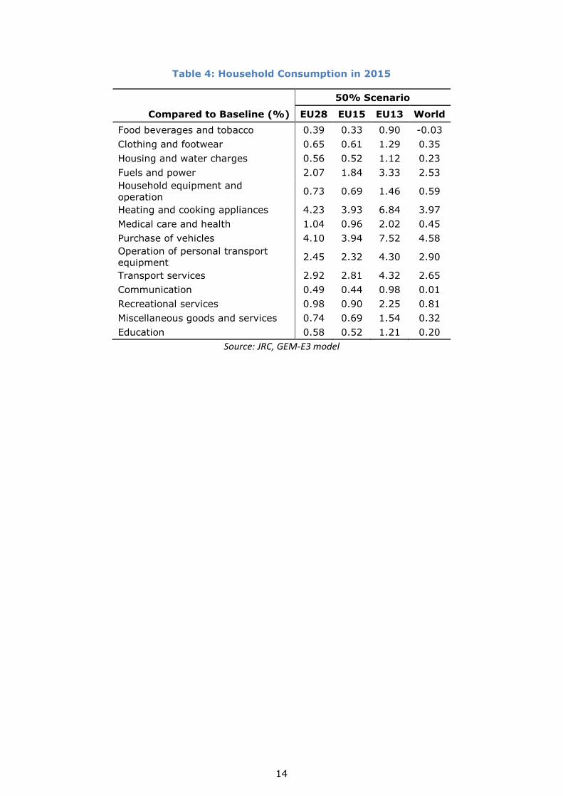
In the global economy, household consumption accounts for 2/3 of the GDP growth, with

investment driving the other 1/3. In the EU28 the household consumption drives about

83% of the GDP growth (and investment still 33%) as part of the growth is neutralized

by a worsened trade balance (-16%) due to a relatively higher increase of imports. The

highest increases can be observed in fuel and heating- and transport-related goods

(Table 4).

14

Table 4: Household Consumption in 2015

50% Scenario

Compared to Baseline (%) EU28 EU15 EU13 World

Food beverages and tobacco 0.39 0.33 0.90 -0.03

Clothing and footwear 0.65 0.61 1.29 0.35

Housing and water charges 0.56 0.52 1.12 0.23

Fuels and power 2.07 1.84 3.33 2.53

Household equipment and

operation 0.73 0.69 1.46 0.59

Heating and cooking appliances 4.23 3.93 6.84 3.97

Medical care and health 1.04 0.96 2.02 0.45

Purchase of vehicles 4.10 3.94 7.52 4.58

Operation of personal transport

equipment 2.45 2.32 4.30 2.90

Transport services 2.92 2.81 4.32 2.65

Communication 0.49 0.44 0.98 0.01

Recreational services 0.98 0.90 2.25 0.81

Miscellaneous goods and services 0.74 0.69 1.54 0.32

Education 0.58 0.52 1.21 0.20

Source: JRC, GEM-E3 model

15

3. Potential short-term evolution of the oil price

3.1 Scenarios

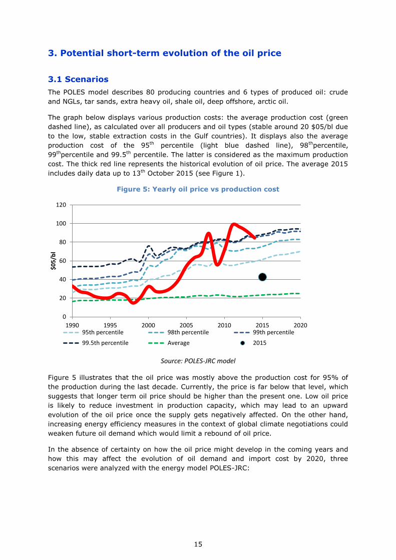
The POLES model describes 80 producing countries and 6 types of produced oil: crude

and NGLs, tar sands, extra heavy oil, shale oil, deep offshore, arctic oil.

The graph below displays various production costs: the average production cost (green

dashed line), as calculated over all producers and oil types (stable around 20 $05/bl due

to the low, stable extraction costs in the Gulf countries). It displays also the average

production cost of the 95th percentile (light blue dashed line), 98thpercentile,

99thpercentile and 99.5th percentile. The latter is considered as the maximum production

cost. The thick red line represents the historical evolution of oil price. The average 2015

includes daily data up to 13th October 2015 (see Figure 1).

Figure 5: Yearly oil price vs production cost

Source: POLES-JRC model

Figure 5 illustrates that the oil price was mostly above the production cost for 95% of

the production during the last decade. Currently, the price is far below that level, which

suggests that longer term oil price should be higher than the present one. Low oil price

is likely to reduce investment in production capacity, which may lead to an upward

evolution of the oil price once the supply gets negatively affected. On the other hand,

increasing energy efficiency measures in the context of global climate negotiations could

weaken future oil demand which would limit a rebound of oil price.

In the absence of certainty on how the oil price might develop in the coming years and

how this may affect the evolution of oil demand and import cost by 2020, three

scenarios were analyzed with the energy model POLES-JRC:

0

20

40

60

80

100

120

1990 1995 2000 2005 2010 2015 2020

$0

5/b

l

95th percentile 98th percentile 99th percentile

99.5th percentile Average 2015

16

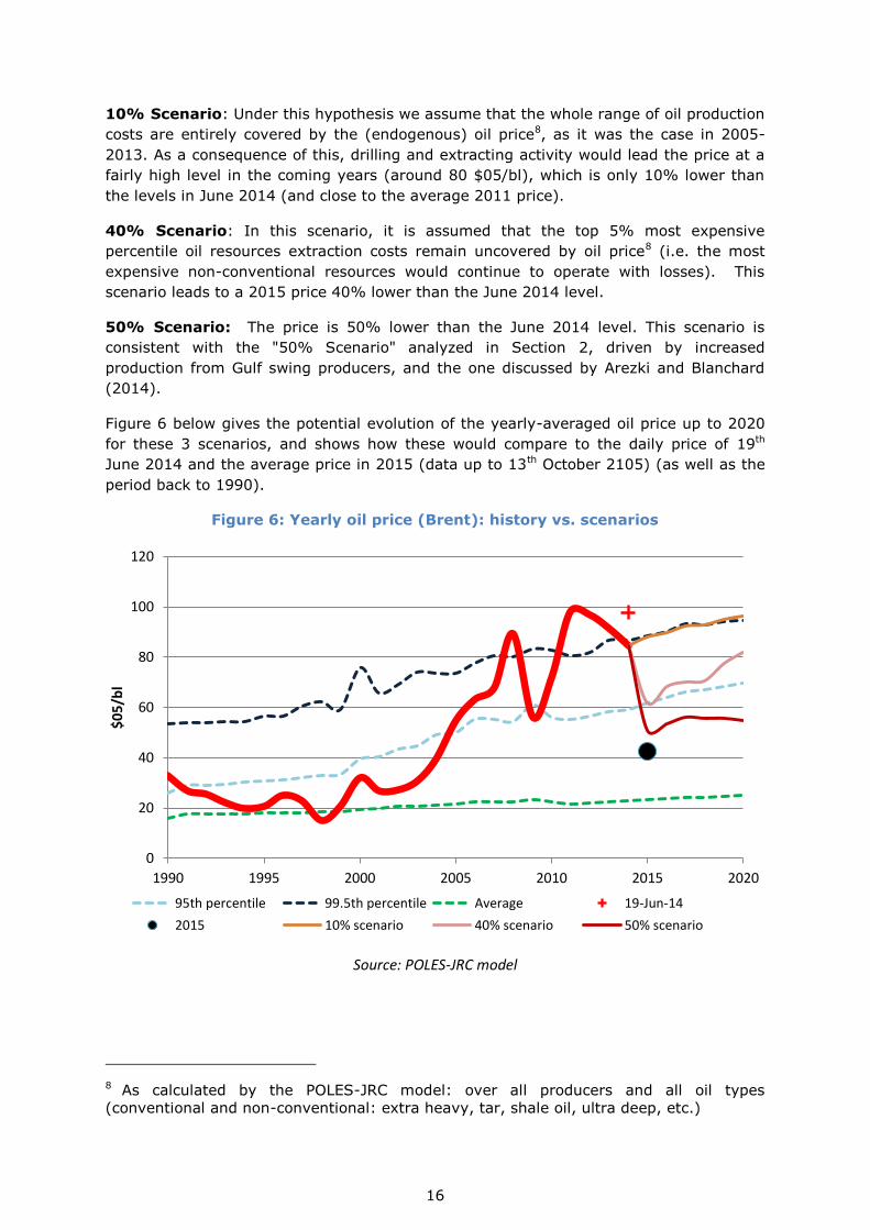
10% Scenario: Under this hypothesis we assume that the whole range of oil production

costs are entirely covered by the (endogenous) oil price8, as it was the case in 2005-

2013. As a consequence of this, drilling and extracting activity would lead the price at a

fairly high level in the coming years (around 80 $05/bl), which is only 10% lower than

the levels in June 2014 (and close to the average 2011 price).

40% Scenario: In this scenario, it is assumed that the top 5% most expensive

percentile oil resources extraction costs remain uncovered by oil price8 (i.e. the most

expensive non-conventional resources would continue to operate with losses). This

scenario leads to a 2015 price 40% lower than the June 2014 level.

50% Scenario: The price is 50% lower than the June 2014 level. This scenario is

consistent with the "50% Scenario" analyzed in Section 2, driven by increased

production from Gulf swing producers, and the one discussed by Arezki and Blanchard

(2014).

Figure 6 below gives the potential evolution of the yearly-averaged oil price up to 2020

for these 3 scenarios, and shows how these would compare to the daily price of 19th

June 2014 and the average price in 2015 (data up to 13th October 2105) (as well as the

period back to 1990).

Figure 6: Yearly oil price (Brent): history vs. scenarios

Source: POLES-JRC model

8 As calculated by the POLES-JRC model: over all producers and all oil types

(conventional and non-conventional: extra heavy, tar, shale oil, ultra deep, etc.)

0

20

40

60

80

100

120

1990 1995 2000 2005 2010 2015 2020

$0

5/b

l

95th percentile 99.5th percentile Average 19-Jun-14

2015 10% scenario 40% scenario 50% scenario

17

3.2 Impact of oil demand and oil imports

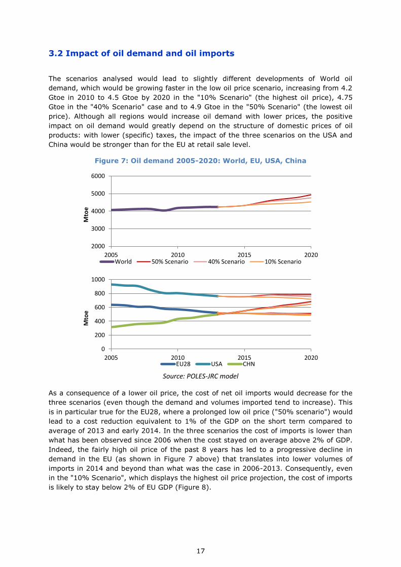
The scenarios analysed would lead to slightly different developments of World oil

demand, which would be growing faster in the low oil price scenario, increasing from 4.2

Gtoe in 2010 to 4.5 Gtoe by 2020 in the "10% Scenario" (the highest oil price), 4.75

Gtoe in the "40% Scenario" case and to 4.9 Gtoe in the "50% Scenario" (the lowest oil

price). Although all regions would increase oil demand with lower prices, the positive

impact on oil demand would greatly depend on the structure of domestic prices of oil

products: with lower (specific) taxes, the impact of the three scenarios on the USA and

China would be stronger than for the EU at retail sale level.

Figure 7: Oil demand 2005-2020: World, EU, USA, China

Source: POLES-JRC model

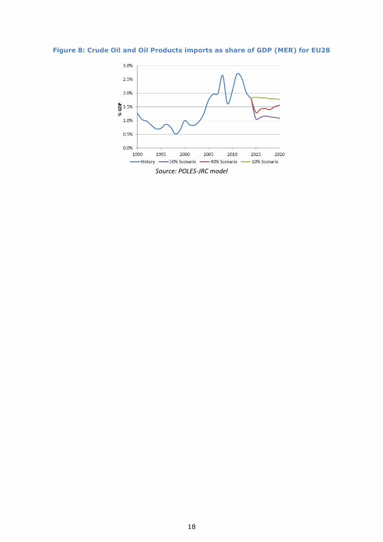
As a consequence of a lower oil price, the cost of net oil imports would decrease for the

three scenarios (even though the demand and volumes imported tend to increase). This

is in particular true for the EU28, where a prolonged low oil price ("50% scenario") would

lead to a cost reduction equivalent to 1% of the GDP on the short term compared to

average of 2013 and early 2014. In the three scenarios the cost of imports is lower than

what has been observed since 2006 when the cost stayed on average above 2% of GDP.

Indeed, the fairly high oil price of the past 8 years has led to a progressive decline in

demand in the EU (as shown in Figure 7 above) that translates into lower volumes of

imports in 2014 and beyond than what was the case in 2006-2013. Consequently, even

in the "10% Scenario", which displays the highest oil price projection, the cost of imports

is likely to stay below 2% of EU GDP (Figure 8).

2000

3000

4000

5000

6000

2005 2010 2015 2020

Mto

e

World 50% Scenario 40% Scenario 10% Scenario

0

200

400

600

800

1000

2005 2010 2015 2020

Mto

e

EU28 USA CHN

18

Figure 8: Crude Oil and Oil Products imports as share of GDP (MER) for EU28

Source: POLES-JRC model

19

4. Conclusions and Caveats

This report describes the importance of oil (imports) for the EU economy and analyses

the potential economic effects of the lower oil price in the EU28. Further it assesses how

the current oil price decrease may evolve up to 2020 and the consequences for global oil

consumption.

The analysis shows that a decrease of the oil price from US$100 to US$50 may lead to a

GDP gain of about 0.7%, both on a global level and in the EU28, driven by private

consumption and investment. The global gains are not evenly distributed. Net oil

importing countries gain, whereas oil exporting countries lose. The analysis mainly

focuses on the EU28 and it shows that the more oil-intensive countries and sectors gain

more than the rest of the economy. A 50% decrease of the oil price may generate up to

3 million additional jobs (1.3% of the total labour force). Interestingly, oil-intensive

sectors do not necessarily improve their competitiveness vis-à-vis their competitors in

other regions, as non-EU producers may be less energy efficient and therefore benefit

more from low oil prices.

The economic analysis is in comparative static terms, i.e. compared to a Baseline and

the results are not projections. The low oil price scenario is ceteris paribus in nature i.e.

the change in oil price is the only difference between the scenario and the Baseline.

Indeed the analysis, does not take into account any policy reactions that may happen

because of this major price shift. Crude oil producers (de facto Saudi Arabia, the main

swing producer) may decide to tighten the oil supply in order to bring the price to higher

levels. Other governments may decide to increase or decrease public spending, or their

tax rates. In fact the IMF (2015a) recommends using the lower oil prices in order to

abolish fuel/energy subsidies which are a major burden on the government budget of

various, mainly developing or emerging, economies. In the analysis presented here, we

assume that all industries in all countries face an identical relative price reduction. As

such, the oil price differential across countries is not assumed to narrow due to a drop in

the oil price. In addition, no changes in the price of other natural resources are imposed

exogenously. This could be relevant especially for natural gas, since long-term gas

contracts may feature oil-indexed price components.

Another caveat is that the methodology does not allow for the appreciation or

depreciation of currencies, changes inflation or interest rate decisions by the central

banks. Finally, the analysis did not consider any dramatic worsening of the situations in

geo-strategically important places like Ukraine or the Middle East.

Furthermore, it should be noted that the economic analysis is of a static nature. Whether

the current oil price is maintainable in the mid- to long-run is uncertain. The last part of

the report shows that the oil price is likely to rise in the coming years to cover the cost

of the most expensive production.

20

References

Arezki, R. and Blanchard, O. (December 2014). "Seven Questions about the Recent Oil

Price Slump," IMF blog post: http://blog-imfdirect.imf.org/2014/12/22/seven-questions-

about-the-recent-oil-price-slump/ (accessed 05/02/2015)

Breitenfellner, A. and Crespo Cuaresma, J. (2008). Crude Oil Prices and the USD/EUR.

Exchange Rate. Monetary Policy & The Economy Q4/08.

Ciscar, J. C., Russ, P., Paroussos, L., and Stroblos, N. (2004). Vulnerability of the EU

Economy to Oil Shocks: A General equilibrium Analysis with the GEM-E3 Model. 13th

annual conference of the European Association of Environmental and Resource

Economics, Budapest, Hungary

IMF (2015a). World Economic Outlook. Update 20 January.

IMF (2015b). IMF Country Report No. 15/286: Saudi Arabia: Selected issues

Kitous, A., Saveyn, B., Gervais, S., Wiesenthal, T., Soria, A. (2013). Analysis of the Iran

oil embargo. JRC Scientific and Technical Reports. EUR 25691 EN.

Maisonnave H, Pycroft J, Saveyn B, Ciscar Martinez J. (2012). Does climate policy make

the EU economy more resilient to oil price rises A CGE analysis. JRC Scientific and

Technical Reports. EUR 25224 EN.

The Economist (December 2014), Why the oil price is falling.

http://www.economist.com/blogs/economist-explains/2014/12/economist-explains-4

(accessed 05/02/2015)

Box: Explanation of units used in this report

TOE Tonne of oil equivalent

Ktoe Kilotonnes of oil equivalent (1000 toe)

Gtoe Gigatonnes of oil equivalent (1'000'000'000 toe)

bl Barrel

bpd Barrels per day

21

List of figures

Figure 1: Daily oil price (Brent, current US$)

Figure 2: Crude oil imports and refineries

Figure 3: Oil products intensity

Figure 4: Impact on GDP of central low oil price scenario for EU28 MS

Figure 5: Yearly oil price vs production cost

Figure 6: Yearly oil price (Brent): history vs. scenarios

Figure 7: Oil demand 2005-2020: World, EU, USA, China

Figure 8: Crude Oil and Oil Products imports as share of GDP (MER) for EU28

22

List of tables

Table 1: Macro-economic impacts of low oil price scenarios in 2015

Table 2: Sectoral Production in 2015

Table 3: Sectoral Employment in 2015

Table 4: Household Consumption in 2015

How to obtain EU publications

Our publications are available from EU Bookshop (http://bookshop.europa.eu),

where you can place an order with the sales agent of your choice.

The Publications Office has a worldwide network of sales agents.

You can obtain their contact details by sending a fax to (352) 29 29-42758.

Europe Direct is a service to help you find answers to your questions about the European Union

Free phone number (*): 00 800 6 7 8 9 10 11

(*) Certain mobile telephone operators do not allow access to 00 800 numbers or these calls may be billed.

A great deal of additional information on the European Union is available on the Internet.

It can be accessed through the Europa server http://europa.eu

2

doi:10.2791/222885

ISBN 978-92-79-52769-2

LF-N

A-2

7537-E

N-N

JRC Mission

As the Commission’s

in-house science service,

the Joint Research Centre’s

mission is to provide EU

policies with independent,

evidence-based scientific

and technical support

throughout the whole

policy cycle.

Working in close

cooperation with policy

Directorates-General,

the JRC addresses key

societal challenges while

stimulating innovation

through developing

new methods, tools

and standards, and sharing

its know-how with

the Member States,

the scientific community

and international partners.

Serving society Stimulating innovation Supporting legislation